Comparative Analysis of Polarimetric SAR Calibration Methods

Abstract

In the diverse applications of polarimetric Synthetic Aperture Radar (SAR) systems, it is a crucial to conduct polarimetric calibration, which aims to remove the radar system distortion effects prior to utilizing polarimetric SAR observations. The objective of this study is to evaluate the performance of different polarimetric calibration methods. Two widely used methods, the Van Zyl and Quegan methods, and one recently proposed method, such as the Villa method, have been selected among various calibration methods in literature. The selected methods have basic differences in their assumptions that are applied to the polarimetric system model. In order to evaluate the calibration performances under different system parameters and ground characteristics, comparative analysis of the calibration results were conducted on synthetic polarimetric SAR data and ALOS PALSAR quad-pol mode data. Based on the experimental results, the advantages and limitations of different methods were clarified, and a simple hybrid calibration method is presented to further improve the polarimetric calibration performance.

1. Introduction

Polarimetric Synthetic Aperture Radar (SAR) measures the vector scattering information of the target, and provides better characterization of the geo- and bio-physical properties of the Earth’s surface. In diverse applications of the polarimetric SAR system, it is crucial to remove the radar system distortion prior to utilizing polarimetric SAR data. The polarimetric calibration aims to correct the system distortion effects in SAR observations by obtaining distortion parameters including cross-talks and channel imbalances. Without proper calibration, distortion could cause the misinterpretation of the intrinsic properties of scatterers or targets.

Based on external targets with known polarimetric scattering properties, several studies have proposed different polarimetric calibration strategies. One of the pioneering works was proposed by Van Zyl [1]. He proposed a calibration method to solve radar system equations based on the natural scatterers’ reflection symmetry assumption and the monostatic radar symmetry assumption. In addition, Freeman et al. [2] relaxed the symmetric radar system assumption adapted in the Van Zyl method. Furthermore, Quegan [3] proposed a non-iterative algorithm without radar symmetry assumption. This method has been used for calibrating air-borne [4] and space-borne [5] polarimetric SAR systems with some modifications. Ainsworth et al. [6] further refined the Quegan method by iteratively solving the system equations with only the weakest of constraints. Recently, a calibration method based on the covariance matching estimation technique was proposed by Villa et al. [7]. It provides a calibration method with numerical optimization, which permits distortion parameters to be obtained without symmetry assumptions of the radar system.

The objective of this study is to compare and evaluate different polarimetric calibration methods, including the Van Zyl method, Quegan method, and Villa method. The selected methods have basic differences in their assumptions that are applied to the polarimetric system model. In order to evaluate the calibration performances under different systems and ground conditions, comparative analyses on the calibration results were conducted, based on the synthetic polarimetric SAR data and the ALOS PALSAR quad-pol mode data. The rest of this study is organized as follows. In Section 2, the definition of the polarimetric distortion problem and a brief review of each method are introduced. Section 3 provides the results of a distortion variability test with synthetic data and performance with ALOS PALSAR data. Lastly, Section 4 and Section 5 contain the discussion and conclusion, respectively.

2. Polarimetric Distortion Problem and Methods

The backscattering properties of a ground scatterer can be completely described by the scattering matrix $\left[S\right]$ defined in the horizontal (H) and vertical (V) polarization basis as:

$$\left[S\right]= \left[\begin{array}{cc}{S}_{HH}& S_{HV}\\ S_{VH}& S_{VV}\end{array}\right].$$

(1)

The actual measurement of the polarimetric SAR system, however, contains some system errors originating during the transmittance and receipt of the signals through the polarization channel modeled by cross-talk and channel imbalance parameters. It is important to define the system model to estimate the distortion parameters as found from the observables. The widely used polarimetric SAR system model [8] represents the measured scattering matrix as:

$$\begin{array}{ll}{\left[\begin{array}{cc}{S}_{HH}& S_{HV}\\ S_{VH}& S_{VV}\end{array}\right]}_{measured}& = {\left[R\right]}^T·\left[S\right]·\left[T\right]+\left[N\right]\\ & =\left[\begin{array}{cc}1& {\delta }_2\\ {\delta }_1& f_1\end{array}\right]{\left[\begin{array}{cc}{S}_{HH}& S_{HV}\\ S_{VH}& S_{VV}\end{array}\right]}_{actual}\left[\begin{array}{cc}1& {\delta }_3\\ {\delta }_4& f_2\end{array}\right]+\left[\begin{array}{cc}{N}_{HH}& N_{HV}\\ N_{VH}& N_{VV}\end{array}\right] ,\hfill \end{array}$$

(2)

where $\left[R\right]$ and $\left[T\right]$ are the receiving and transmitting distortion matrices, respectively, and $\left[N\right]$ is the additive noise matrix. The distortion matrix contains complex-valued distortion parameters, such as the channel imbalances $f_1$ and $f_2$, and the cross-talk terms ${\delta }_1$, ${\delta }_2$, ${\delta }_3$, and ${\delta }_4$. It is worth noting that the ionospheric propagation effect is neglected in this study. The system model can be rewritten in a vector form as follows [9]:

$${\overrightarrow{S}}_{measured}=\left[D\right]·{\overrightarrow{S}}_{actual},$$

(3)

$$\left[D\right]={\left[T\right]}^T\otimes {\left[R\right]}^T= \left[\begin{array}{cccc}1& {\delta }_2& {\delta }_4& {\delta }_2{\delta }_4\\ {\delta }_1& f_1& {\delta }_1{\delta }_4& {\delta }_4{f}_1\\ {\delta }_3& {\delta }_2{\delta }_3& f_2& {\delta }_2{f}_2\\ {\delta }_1{\delta }_3& {\delta }_3{f}_1& {\delta }_1{f}_2& f_1{f}_2\end{array}\right],$$

(4)

where $\left[D\right]$ is a single matrix that the distortion parameters are signified, and $\otimes$ denotes the Kronecker product.

2.1. Van Zyl Method

In the Van Zyl method [1], the system model is simplified by neglecting the noise term, and by assuming radar system symmetry $\left[R\right]=\left[T\right]$, such as:

$${\left[\begin{array}{cc}{S}_{HH}& S_{HV}\\ S_{VH}& S_{VV}\end{array}\right]}_{measured}=\left[\begin{array}{cc}1& {\delta }_2\\ {\delta }_1& f\end{array}\right]{\left[\begin{array}{cc}{S}_{HH}& S_{HB}\\ S_{VH}& S_{VV}\end{array}\right]}_{actual}\left[\begin{array}{cc}1& {\delta }_1\\ {\delta }_2& f\end{array}\right].$$

(5)

The distortion matrices can be separated into two components as [10]:

$$\begin{gathered} \left[T\right]=\left[\begin{array}{cc}1& 0\\ 0& f\end{array}\right]\left[\begin{array}{cc}1& {\delta }_1\\ {\delta }_2/f& 1\end{array}\right] = \left[T_C] [T_X\right], \\ {\left[R\right]}^T= \left[\begin{array}{cc}1& {\delta }_2/f\\ {\delta }_1& 1\end{array}\right]\left[\begin{array}{cc}1& 0\\ 0& f\end{array}\right] = \left[R_X] [R_C\right], \end{gathered}$$

(6)

where subscripts $X$ and $C$ represent the cross-talk and the channel imbalance components, respectively. Then, the system equation can be rewritten as:

$$\begin{array}{ll}{\left[S\right]}_{measured}& =\left[R_X] [R_C\right]{\left[S\right]}_{actual}\left[T_C] [T_X\right]\\ & =\left[R_X\left] \left[W\right] \right[T_X\right]\end{array}$$

(7)

Since the channel imbalance components have no relation to the system cross-talks, it is possible to solve the simplified system equation by a two-step inversion approach. Firstly, the cross-talk components can be estimated iteratively on the basis of the reflection symmetry assumption of the natural distributed target. Then, the channel imbalance component is estimated by using the external calibration target, such as the trihedral corner reflector (CR).

2.2. Quegan Method

Without the radar system symmetry assumption, the Quegan method [3] assumes the general system model, which can be rewritten in a vector form that is equivalent to Equation (4). The distortion matrix [M] in the Quegan method looks slightly different than (4). It contains the ratios of the receiving and transmittance channel distortion parameters as:

$$\left[M\right]= Y\left[\begin{array}{cccc}1& w& v& vw\\ u& 1& uv& v\\ z& wz& 1& w\\ uz& z& u& 1\end{array}\right]\left[\begin{array}{cccc}a{k}^2& 0& 0& 0\\ 0& ak& 0& 0\\ 0& 0& k& 0\\ 0& 0& 0& 1\end{array}\right],$$

(8)

where $Y$ is the overall system gain, $u, v, z, w$ are the cross-talk ratios, $\alpha$ is the ratio of the receiving and transmittance channel imbalances, and $k$ is the receiving channel imbalance.

Based on the vectorial system model and the azimuthally symmetric target, the observed covariance matrix is given by:

$$\begin{gathered} {\left[C\right]}_{measured} =\mathrm{Y}·\left[\mathrm{M}\right]·{\left[C\right]}_{actual}·{\left[\mathrm{M}\right]}^{*T} \\ {\left[C\right]}_{actual}=\left[\begin{array}{ccc}{\langle \left|S_{HH}\right|}^2\rangle & 0& \langle S_{HH}{S}_{VV}^{*}\rangle \\ 0& 2{\langle \left|S_{HV}\right|}^2\rangle & 0\\ \langle S_{VV}{S}_{HH}^{*}\rangle & 0& {\langle \left|S_{VV}\right|}^2\rangle \end{array}\right], \end{gathered}$$

(9)

The system model permits to derivation of a set of equations to solve the cross-talk terms and $\alpha$ as:

$$\begin{gathered} u=\left(C_{44}{C}_{21}-C_{41}{C}_{24}\right)/\left(C_{11}{C}_{44}-C_{14}{C}_{41}\right) \\ v=\left(C_{11}{C}_{24}-C_{21}{C}_{14}\right)/\left(C_{11}{C}_{44}-C_{14}{C}_{41}\right) \\ z=\left(C_{44}{C}_{31}-C_{41}{C}_{34}\right)/\left(C_{11}{C}_{44}-C_{14}{C}_{41}\right) \\ w=\left(C_{11}{C}_{34}-C_{31}{C}_{14}\right)/\left(C_{11}{C}_{44}-C_{14}{C}_{41}\right) \\ {\alpha }^{*}=\frac{C_{32}-u^{*}\left(z{C}_{11}+w{C}_{41}\right)-v^{*}\left(z{C}_{14}+w{C}_{44}\right)}{C_{33}-z^{*}\left(z{C}_{11}+w{C}_{41}\right)-w^{*}\left(z{C}_{14}+w{C}_{44}\right)} \end{gathered}$$

(10)

The channel imbalance components can be estimated using the external calibration target after the cross-talk components are calibrated.

2.3. Villa Method

The polarimetric system model in the Villa method [7] is commenced from the general system model without the symmetry assumption of the radar system given in Equation (2). The covariance matrix of the expected observation ${\left[C\right]}_{inv}$ with the distortion parameters is then represented as:

$${\left[C\right]}_{inv}=\left[H\right]·\left[C_S\right]·{\left[H\right]}^{*T}+{\sigma }_{N}I,$$

(11)

where $*T$ denotes the conjugate transpose, $\left[H\right]$ is the same matrix as $\left[D\right]$ in Equation (4), and $\left[C_S\right]$ is the covariance matrix of distributed scatterers with no calibration errors. $\left[C_S\right]$ is defined as:

$$\left[C_S\right]=\left[\begin{array}{cccc}{\mathsf{\sigma }}_{HH}& 0& 0& \rho \\ 0& {\mathsf{\sigma }}_{HV}& {\mathsf{\sigma }}_{HV}& 0\\ 0& {\mathsf{\sigma }}_{HV}& {\mathsf{\sigma }}_{HV}& 0\\ {\rho }^{*}& 0& 0& {\mathsf{\sigma }}_{vv}\end{array}\right].$$

(12)

where ${\mathsf{\sigma }}_{HH}={\langle \left|S_{HH}\right|}^2\rangle ,{ \mathsf{\sigma }}_{HV}={\langle \left|S_{HV}\right|}^2\rangle , {\mathsf{\sigma }}_{VV}={\langle \left|S_{VV}\right|}^2\rangle$ and $\rho =\langle S_{HH}{S}_{VV}^{*}\rangle$. Instead of solving the system model directly, the distortion parameters can be estimated by the means of numerical optimization. The formula of the numerical optimizer for the covariance matrix of the measured ${\left[C\right]}_{data}$ to match with the reconstructed ${\left[C\right]}_{inv}$ is then eventually expressed as follows:

$$\widehat{f},\widehat{\delta }=argmi{n}_{H\left(\widehat{f},\widehat{\delta }\right),C_S\left(\widehat{\sigma },\widehat{\rho }\right)} \parallel W^{-1/2}·({\overrightarrow{C}}_{data}-{\overrightarrow{C}}_{inv}\left(H,C_S\right))\parallel ,$$

(13)

where $\widehat{\sigma },\widehat{\rho }$ are the estimates of the optimizer, and $W$ is the weighting function as below:

$$W=\frac{1}{N}·({\left[C\right]}_{data}^T\otimes {\left[C\right]}_{data}).$$

(14)

With the Hessian optimizer, the final estimates $\widehat{f},\widehat{\delta }$ should be the result that most closely matches the expected covariance matrix ${\left[C\right]}_{inv}$ to the data covariance matrix using covariance matching technique [7].

3. Experimental Results

3.1. Experiment with Simulated Data

In order to compare the calibration performance of the aforementioned different methods, simulations of uncalibrated covariance matrix with varying system distortion conditions were used as the first experiment. Variations of the amplitude and phase values of cross-talks and channel imbalances for analyzing the influence of distortion parameters were summarized in

Table 1. The considered distortion parameters for simulation data.

Distortion Parameters		Unit	Value
Cross-talk	Amplitude	[dB]	[−40 : 5 : −25]
	Phase	[deg]	[∠−120 : ∠60 : ∠120]
Channel imbalance	Amplitude	[dB]	[−2 : 2 : 2]
	Phase	[deg]	[∠−20, ∠0, ∠20]

.

Under the given distortion conditions, the synthetic covariance matrix was generated according to the general system model, such as:

$${\left[C\right]}_{synthetic data}=\left[D\right]{[C]}^{ideal}{\left[D\right]}^{*T}+{\sigma }_{N}I.$$

(15)

The additive thermal noise contribution ${\sigma }_N$ considered here was −30dB. Two groups of ideal targets, such as the azimuthally symmetric distributed target (DT) and the corner reflector (CR), were considered to perform polarimetric calibrations. For the ideal covariance matrix of the DT, the volume scattering covariance matrix corresponding to randomly oriented dipoles [11] was selected. For the simulation of CR responses, the covariance matrix of the trihedral corner reflector was used. The ideal covariance matrices of DT and CR are as given in Equation (16):

$${\left[C\right]}_{DT}^{ideal}=\frac{1}{8}\left[\begin{array}{cccc}3& 0& 0& 1\\ 0& 1& 1& 0\\ 0& 1& 1& 0\\ 1& 0& 0& 3\end{array}\right],{[C]}_{CR}^{ideal}=\frac{1}{2}\left[\begin{array}{cccc}1& 0& 0& 1\\ 0& 0& 0& 0\\ 0& 0& 0& 0\\ 1& 0& 0& 1\end{array}\right].$$

(16)

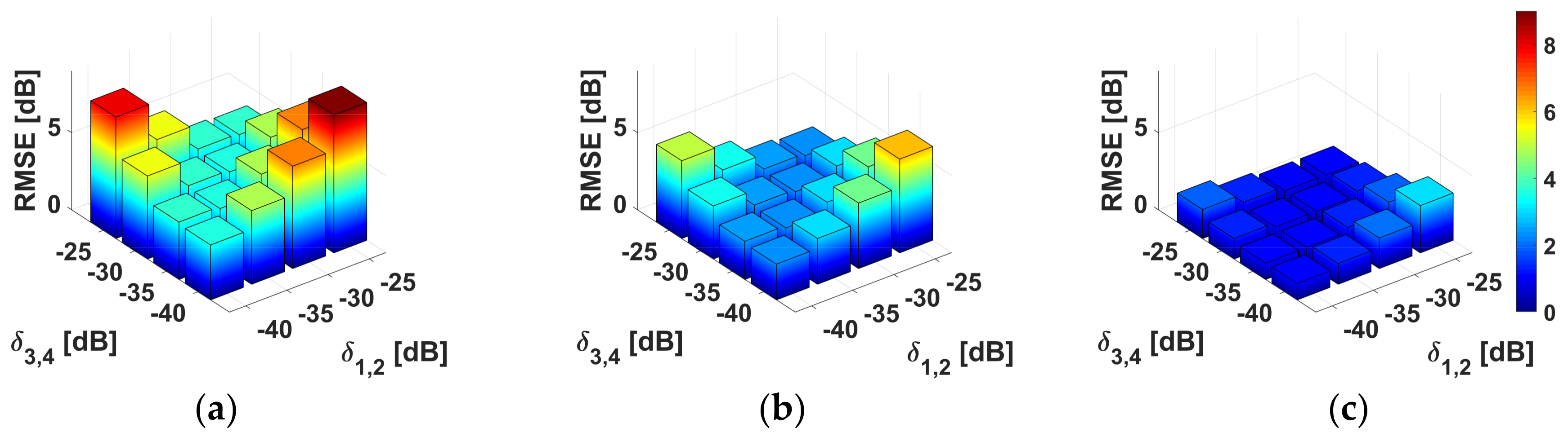
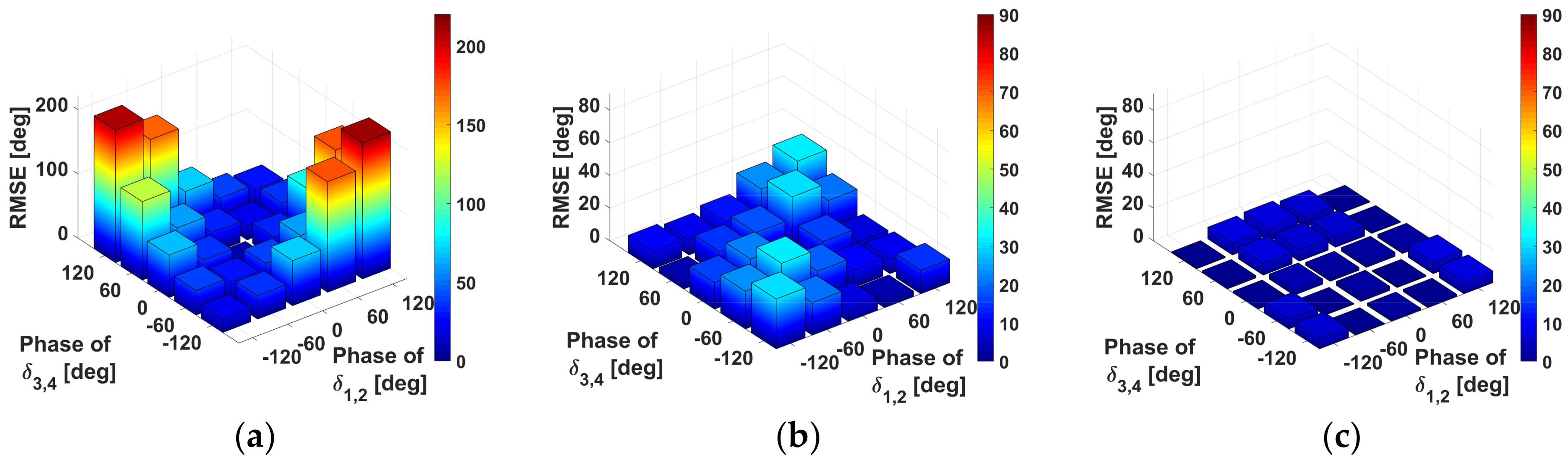
The performance of cross-talk estimation of each calibration method was firstly examined, based on the synthetic uncalibrated data with varying cross-talk parameters. The accuracy was evaluated based on the root mean square error (RMSE) between the true and estimated cross-talk parameters. Figure 1 and Figure 2 show the accuracy assessment results for amplitude and phase of the cross-talk parameters, respectively. As expected from the radar symmetry assumption, RMSE of the Van Zyl method increased as an increase of the relative difference between receiving (${\delta }_{1,2}$) and transmitting (${\delta }_{3,4}$) cross-talks, as shown in Figure 1a and Figure 2a. Since the Quegan method does not assume the radar symmetry, cross-talk estimation results showed relatively lower RMSE than those obtained by the Van Zyl method, as shown in Figure 1b and Figure 2b. However, the cross-talk estimation of the Quegan method was still affected by the asymmetric cross-talks between the transmitting and receiving radar systems. On the other hand, Figure 1c and Figure 2c show that cross-talk estimation results from the Villa method provided lower overall RMSE values, and they were barely affected by the difference between the given cross-talks.

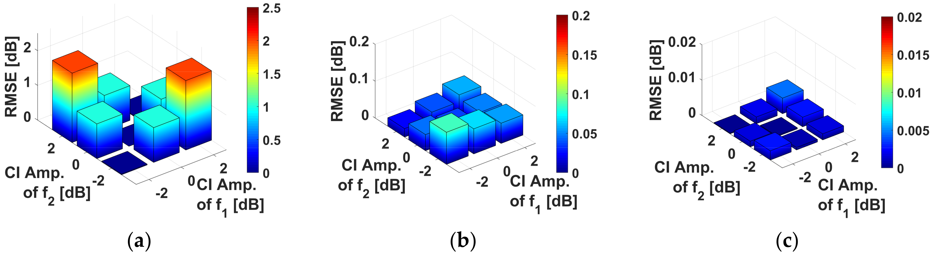
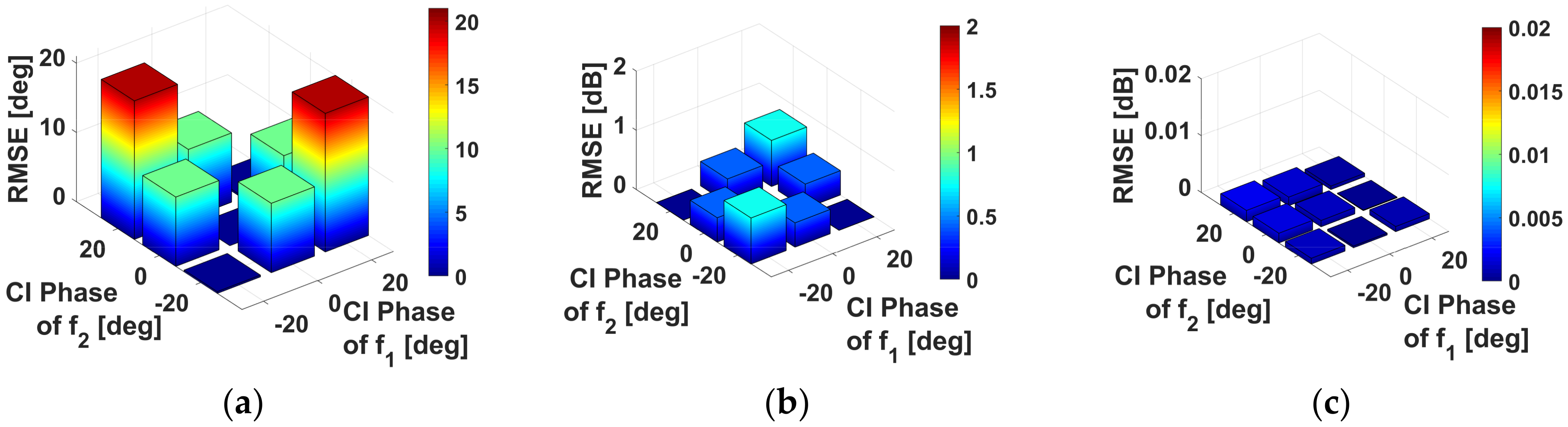
Figure 3 and Figure 4 show the performance analysis results for the estimation of channel imbalances with simulated response of trihedral CR. Both the amplitude and the phase of estimation of the channel imbalance parameter showed similar patterns. In short, the Van Zyl method provided relatively higher RMSE, while the Quegan and Villa methods showed much lower RMSE.

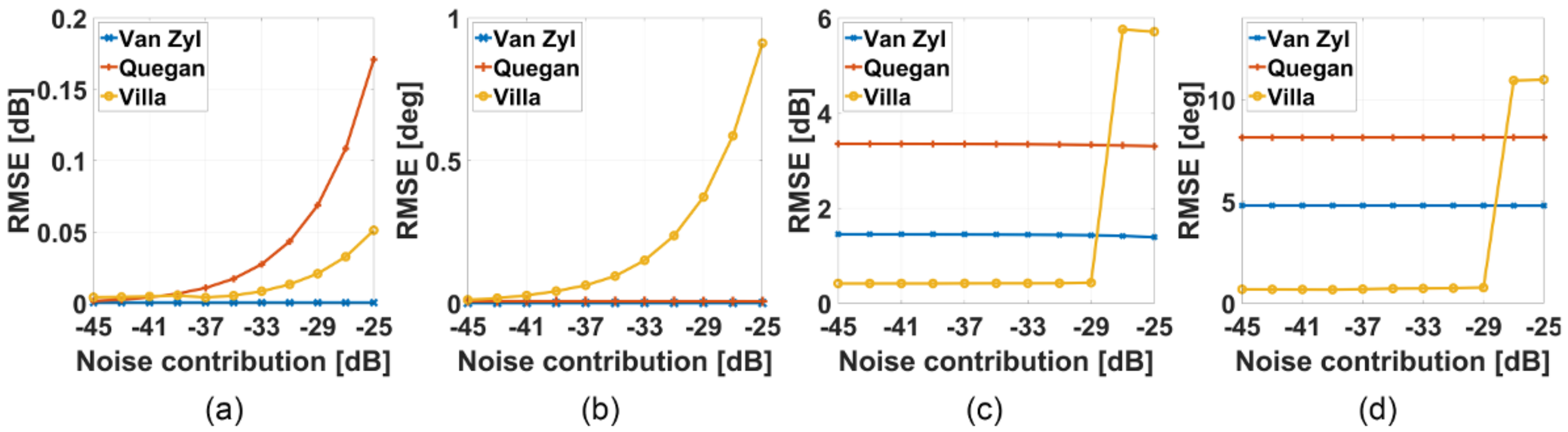
Since the noise term in (15) cannot be removed from the measurement, we also conducted an additional experiment to evaluate the effect of additive noise on the calibration performance of each calibration method. The noise terms are assumed to be uncorrelated with each other, and with signal terms [12]. Figure 5 shows the influence of additive noise contribution on the estimation of distortion parameters. Here, all cross-talks were set to be $-30\mathrm{dB}\angle 20°$, and channel imbalances were $f_1=2\mathrm{dB}\angle 20°$ and $f_2=-2\mathrm{dB}\angle 20°$. Since the additive noise mainly affect the measured backscatter intensities, RMSE of estimated channel imbalances increased as an increase of noise contribution. Both the amplitude and phase of channel imbalance estimation by the Villa method were more influenced by the noise than by other methods. In the case of cross-talk estimation, most methods were not affected by the variation of additive noise. However, significant noise-induced errors in cross-talk estimation by the Villa method can be identified if the additive noise becomes larger than the system crosstalk value.

3.2. Experiments on Real Data

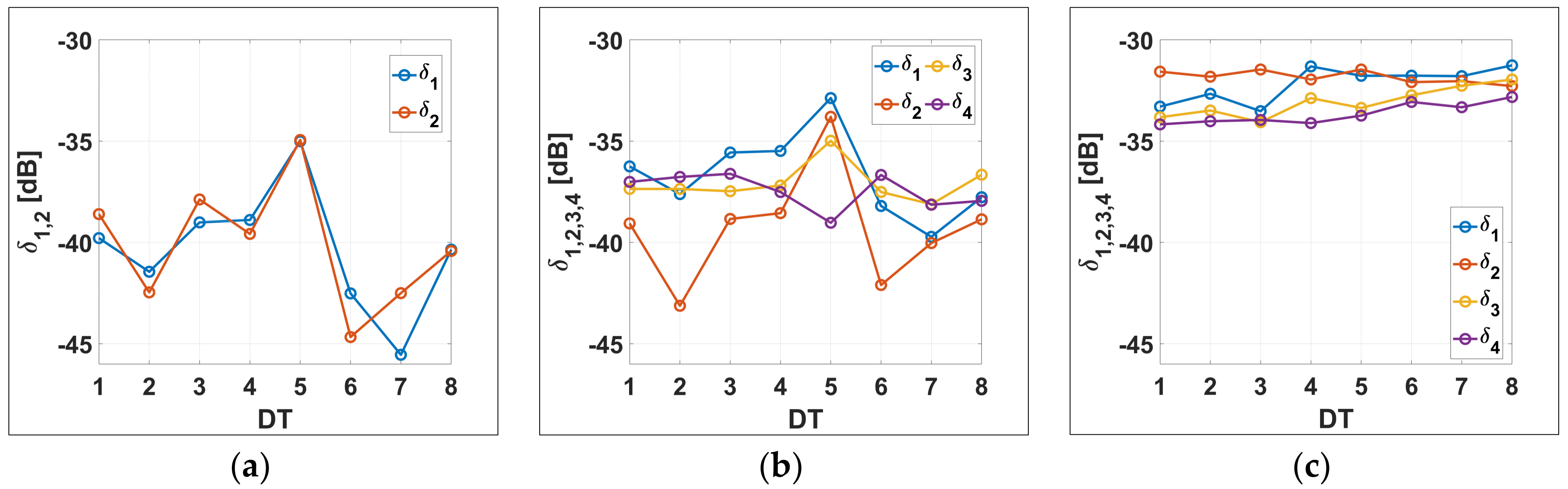
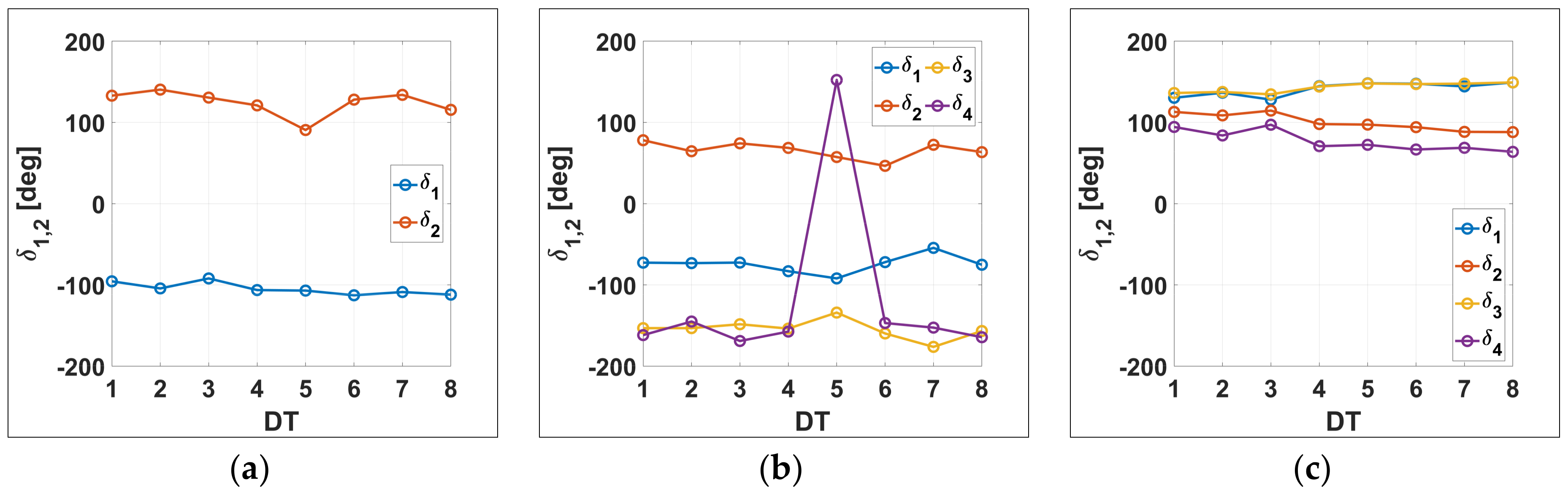
The second experiment was conducted on a real data set, acquired by the ALOS PALSAR over Rio Branco in Amazon area on 20 July 2006. Figure 6 shows the Pauli image of the PALSAR data. The numbers in Figure 6 are eight selected DT (rainforests) for investigating polarimetric calibration methods. The triangle on Figure 6 represents the location of the trihedral CR that has been used for the calibration of the PALSAR polarimetric mode data [5].

Figure 7 and Figure 8 show the results of cross-talk estimation from each calibration method by using the selected DTs. Although DTs selected in the study area were sampled from the similar Amazonian rainforest areas, the Van Zyl and Quegan methods showed significant variations in the cross-talk estimation, as shown in Figure 7a,b. Figure 7c shows that the Villa method provided stable estimates of cross-talk amplitudes of about −32 dB to −35 dB. For the estimation of the cross-talk phase, the Van Zyl and Quegan methods provided rather stable estimates of phase values than in the case of amplitude estimation. Nonetheless, the Villa method gave the most stable results in the cross-talk phase estimation as well. The experimental results indicate that the Van Zyl and Quegan methods could be influenced by the variation in calibration targets, while the optimization-based method could accommodate the observational variabilities.

Figure 9 shows the results of channel imbalance estimation from each calibration method. Since all methods considered the contribution of CR observations, estimation results were exhibited to be rather steady, in contrast with the results from the cross-talk estimation. The amplitude and phase values estimated from the Van Zyl method were close to the mean value of transmitting and receiving channel imbalances as estimated from the Quegan method. The estimated channel imbalance amplitudes from the Quegan and Villa methods were similar to each other, while the phase estimates were quite different between the two methods. To have a better understanding of the differences between Quegan and Villa methods, an additional experiment is presented in the next section.

4. Discussion

Two groups of experiments discussed the performance of different polarimetric calibration methods. Experimental results based on the synthetic data showed a clear advantage of the use of numerical optimizer, based on the covariance matching technique in estimating distortion parameters. Under simulational conditions, the Villa approach provided almost precise estimates of given distortion configurations. On the other hand, since it is not possible to know the true distortion parameters of real SAR systems, the calibration results in the experiments with real data are still not clear. In order to further evaluate the performance of calibration methods, we analyzed the polarimetric characteristics of the CR after applying the distortion matrices that were obtained from each calibration method.

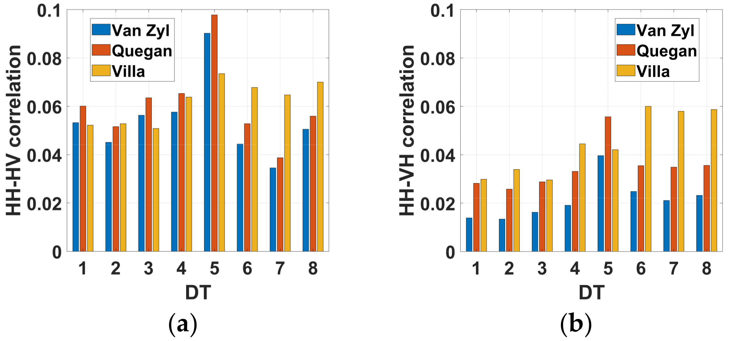
First, the correlation between co- and cross-polarization channels of the CR response were investigated. They should be zero in the case of the ideally calibrated target. Figure 10a,b show the correlation between HH- and HV-polarizations (HH-HV correlation), and the correlation between HH- and VH-polarizations (HH-VH correlation), respectively. Here, polarimetric calibration was applied using distortion parameters obtained from each DT. All calibration methods made the correlation terms close to zero. However, there were some systematic differences between HH-HV and HH-VH correlations, particularly in the Van Zyl and Quegan calibration results. In the Villa method, the levels of co- and cross-pol correlation were increased for some DTs, but the differences between HH-HV and HH-VH correlation were relatively low.

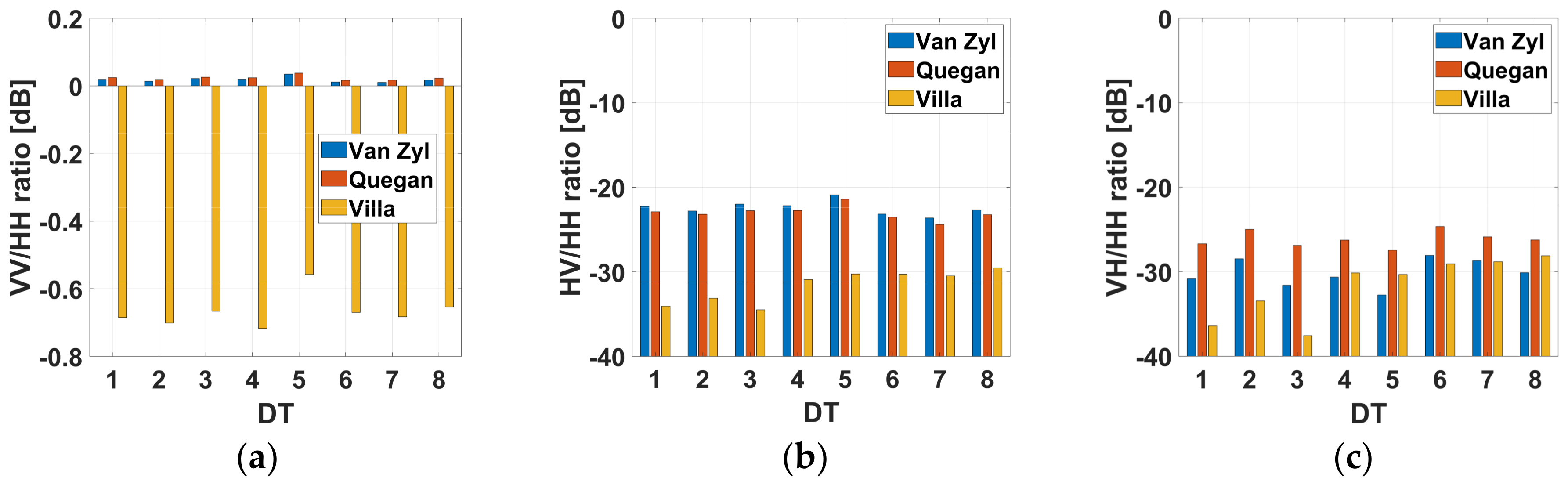
Second, the co-polarization scattering power ratio (VV/HH) and the cross-polarization to co-polarization power ratios (HV/HH and VH/HH) of the calibrated CR response were examined as shown in Figure 11. Figure 11a shows that the VV/HH ratios of CR calibrated by the Van Zyl and Quegan methods became close to 1, whereas there was a difference between the VV and HH scattering powers in the case of the Villa method. On the other hand, the Villa method provided the lowest HV/HH and VH/HH ratios among different methods, and the relative differences between HV and VH polarizations were low.

The overall experimental evaluation indicates that each method has its own advantages and disadvantages. The Van Zyl and Quegan methods could calibrate the imbalance of ratio between the HH and VV polarization, while the HV- and VH-related terms might be not sufficiently calibrated, and the estimated cross-talk parameters could be significantly affected by the targets’ variability. On the other hand, the Villa method provided stable solutions for the distortion parameters, but it might excessively optimize co- and cross-polarization correlation terms to be zero, resulting in the imbalances between HH and VV channels. The actual covariance matrix of the random forests can be different from the ideal reflection symmetric covariance matrix, and they can contain non-zero co- and cross-polarization correlation values. In this case, the reflection symmetry constraint in the calibration model may lead to poor parameter estimates.

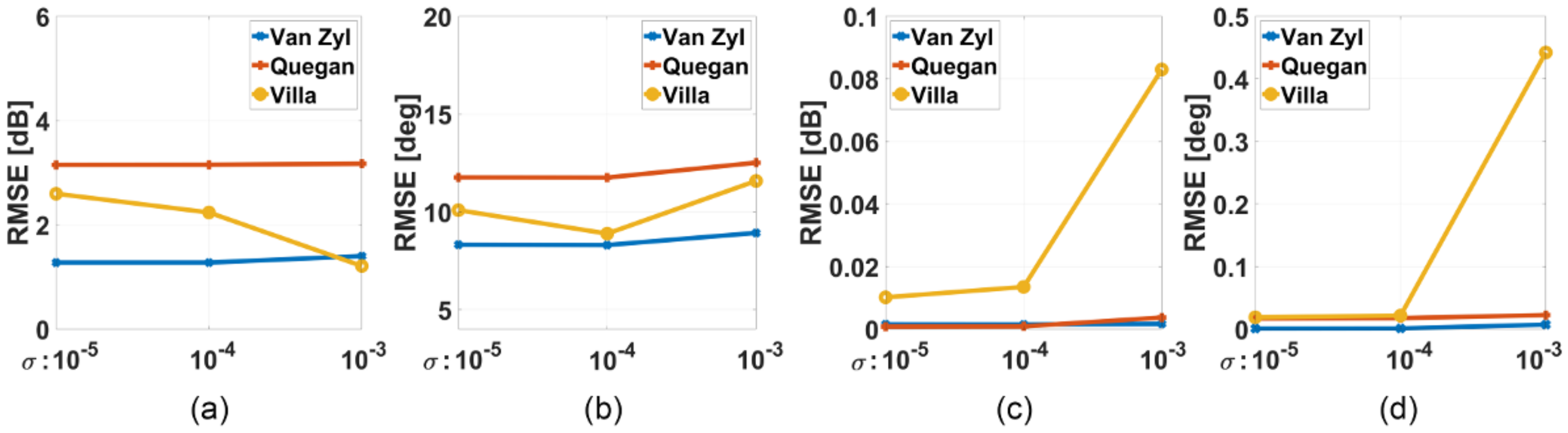
In order to illustrate the influence of non-reflection symmetry on the estimation of distortion parameters, an additional simulation study was carried out. In this experiment, the synthetic data generated by the equation (15) were designed to be non-reflection symmetric by adding small complex values in the co- and cross-polarization correlation terms, such as:

$${\left[C_S\right]}_N=\left[\begin{array}{cccc}3/8& \sigma n_1& \sigma n_2& 1/8\\ \sigma n_3& 1/8& 1/8& \sigma n_4\\ \sigma n_5& 1/8& 1/8& \sigma n_6\\ 1/8& \sigma n_7& \sigma n_8& 3/8\end{array}\right]$$

(17)

where $n_k$ is from zero-mean complex Gaussian random numbers with the standard deviation of $\sigma$ for simulating the non-reflection symmetric covariance matrix. Figure 12 show the variation of calibration accuracies with respect to the amount of non-zero co- and cross-polarization correlation terms. As the contribution of co- and cross-polarization correlation terms increased, errors in the channel imbalance estimates from the Villa method were increased. It indicates that problems in the channel imbalance estimation from the optimization based approach can be attributed to the overfitting of co- and cross-polarization correlation terms to be zero.

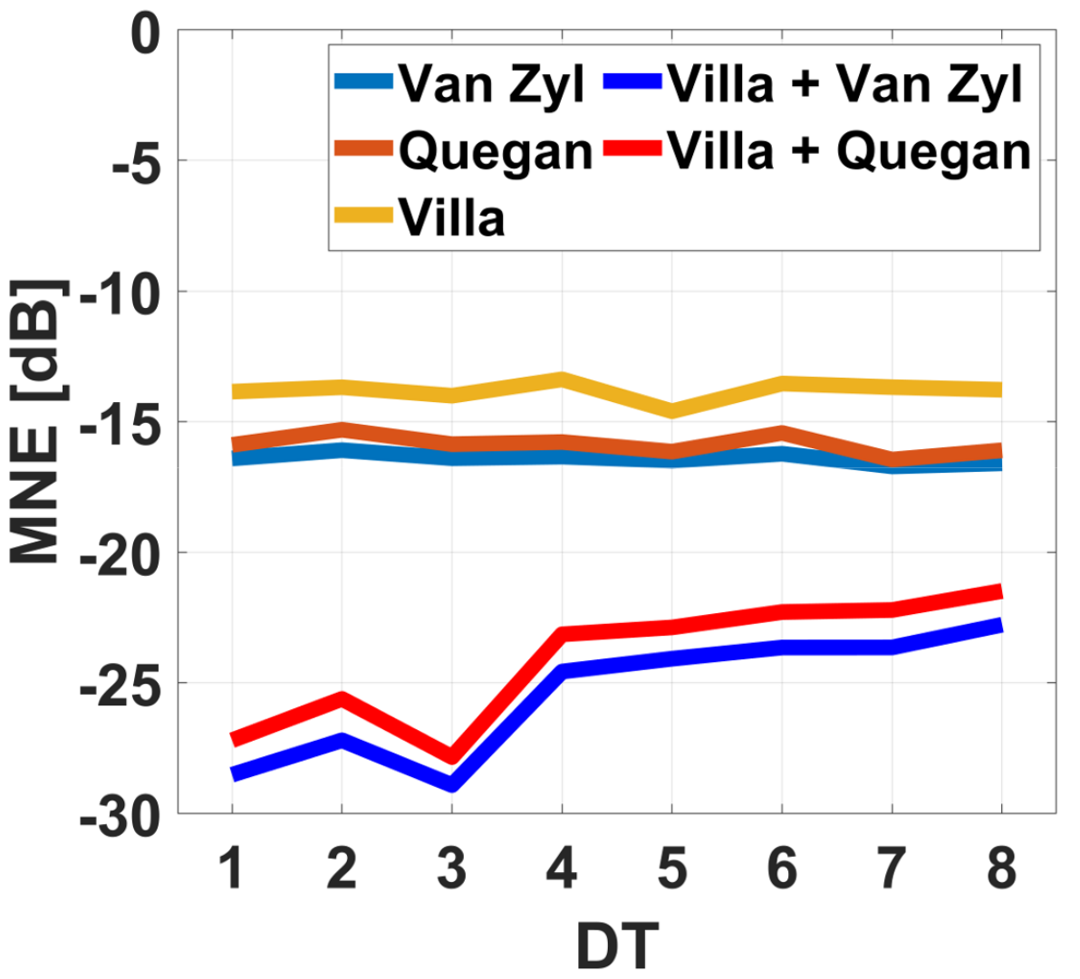
Instead of explicitly addressing these issues by improving system models in the calibration, one may consider a simple combination of different calibration approaches to improve calibration performance. Based on experimental results, a simple hybrid calibration approach was proposed, such as estimating cross-talks by the Villa method, and channel imbalances by the Van Zyl or Quegan methods. The overall calibration performance was then evaluated by a new covariance matrix similarity metric named the maximum normalized error (MNE), represented as [13]:

$$MNE=\sqrt{{\lambda }_{max}({\left[A\right]}_4^{*T}·{({\left[C\right]}_{CR}^{theory}-{\left[C\right]}_{CR}^{calibrated})}^{*T}·({\left[C\right]}_{CR}^{theory}-{\left[C\right]}_{CR}^{calibrated})·{\left[A\right]}_4)},$$

(18)

where, ${\lambda }_{max}$ is the largest eigenvalue of the following matrix, and $\left[A\right]$ is a matrix as follows:

$$\left[A\right]=\left[\begin{array}{ccc}1& 0& 0\\ 0& 1& 0\\ 0& 1& 0\\ 0& 0& 1\end{array}\right],$$

(19)

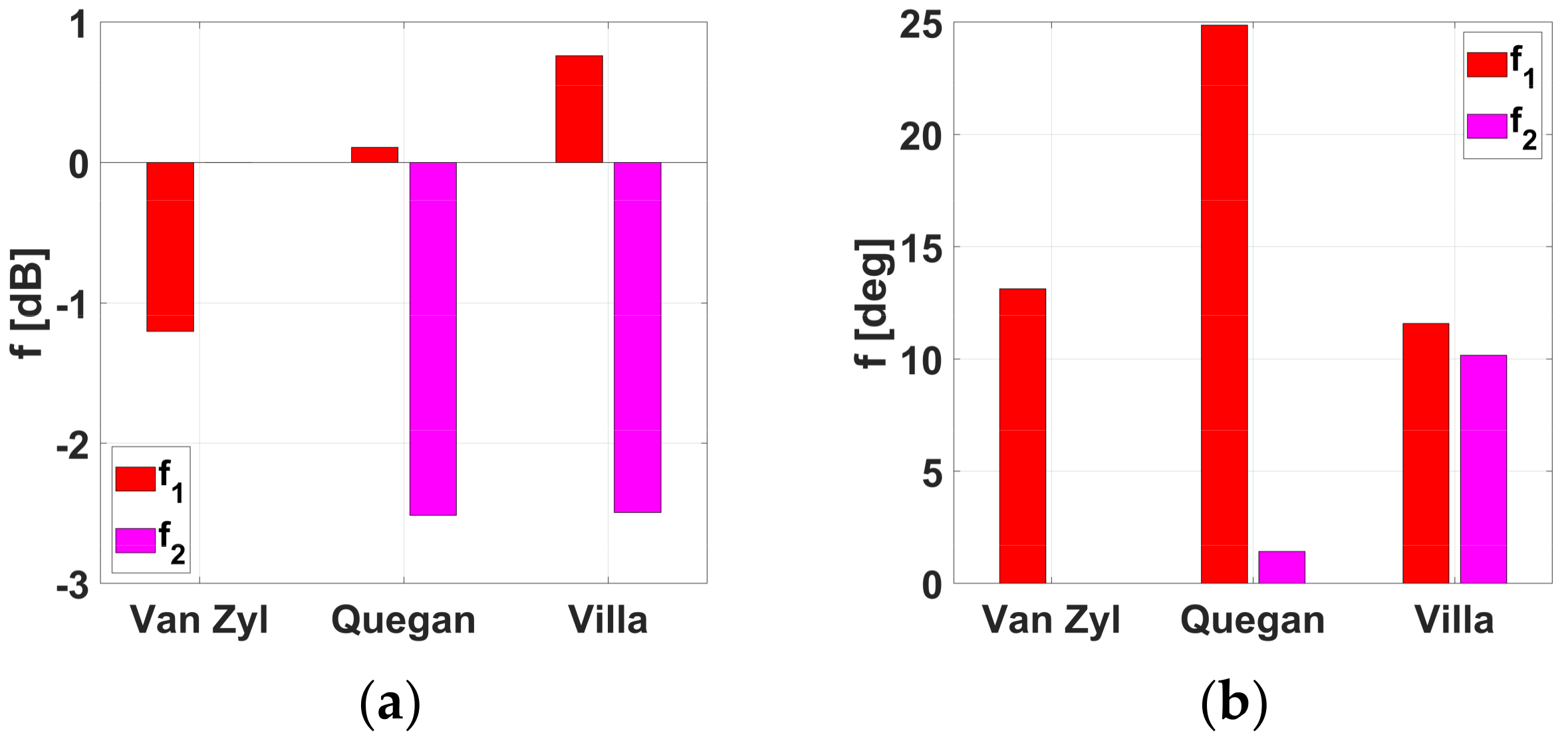
Figure 13 shows the performance evaluation results of the different calibration methods through the MNE. The average MNE values of Van Zyl, Quegan, and Villa methods were about −16.41 dB, −15.87 dB, and −13.8 dB, respectively. The symmetry assumption of SAR system might not suitable for reflecting real system characteristics, but appeared to be effective in estimating channel imbalances, which showed lower MNE in Van Zyl and Quegan methods. Both hybrid approaches, such as Villa+Zyl and Vill+Quegan methods, outperformed previous methods with much lower MNE values around −25.43 dB and −24.09 dB, respectively.

5. Conclusions

A comprehensive comparison of different polarimetric calibration methods, including the Van Zyl, Quegan, and Villa methods, is presented in this study. Firstly, the estimation of the distortion parameters using synthetic data has been discussed. With the presence of asymmetry between transmitting and receiving systems’ cross-talks, the Van Zyl and Quegan methods showed higher estimation errors, while the Villa method could accommodate such conditions with a numerical optimizer. In estimating channel imbalances, both the Quegan and Villa methods provided almost exact estimates under simulation conditions.

In addition to the synthetic data, a real ALOS PALSAR data acquired over the Amazonian forest was used for assessing calibration performances. Unlike the Van Zyl and Quegan methods, stable estimates of the distortion parameters could be obtained by the Villa method, regardless of the sampling location of the distributed targets. It is expected that optimization-based calibration can provide reliable results for long-term system management by minimizing influence of targets’ variability in the calibration process. However, the optimization can be problematic in some conditions and causes an imbalance between HH and VV channels. To overcome limitations in each calibration method, one may consider a combination of different approaches. Based on the characteristics of different calibration methods, a hybrid calibration strategy is tested. It provides a potential improvement of calibration results with higher overall agreement between the theoretical and the calibrated target’s response.

References

- Van Zyl, J.J. Calibration of polarimetric radar images using only image parameters and trihedral corner reflector responses. IEEE Trans. Geosci. Remote Sens. 1990, 28, 337–348. [Google Scholar] [CrossRef]
- Freeman, A.; Van Zyl, J.J.; Klein, J.D.; Zebker, H.A.; Shen, Y. Calibration of Stokes and scattering matrix format polarimetric SAR data. IEEE Trans. Geosci. Remote Sens. 1992, 30, 531–539. [Google Scholar] [CrossRef]
- Quegan, S. A unified algorithm for phase and cross-talk calibration of polarimetric data-theory and observations. IEEE Trans. Geosci. Remote Sens. 1994, 32, 89–99. [Google Scholar] [CrossRef]
- Ainsworth, T.L.; Ferro-Famil, L.; Lee, J.S. Orientation angle preserving a posteriori polarimetric SAR calibration. IEEE Trans. Geosci. Remote Sens. 2006, 44, 994–1003. [Google Scholar] [CrossRef]
- Kimura, H.; Mizuno, T. Improvement of polarimetric SAR calibration based on the Quegan algorithm. In Proceedings of the IGARSS 2004—IEEE International Geoscience and Remote Sensing Symposium, Anchorage, AK, USA, 20–24 September 2004; pp. 184–187. [Google Scholar]
- Shimada, M.; Isoguchi, O.; Tadono, T.; Isono, K. PALSAR radiometric and geometric calibration. IEEE Trans. Geosci. Remote Sens. 2009, 47, 3915–3932. [Google Scholar] [CrossRef]
- Villa, A.; Iannini, L.; Giudici, D.; Monti-Guarnieri, A.; Tebaldini, S. Calibration of SAR polarimetric images by means of a covariance matching approach. IEEE Trans. Geosci. Remote Sens. 2015, 53, 674–686. [Google Scholar] [CrossRef]
- Barnes, R.M. Polarimetric Calibration Using In-Scene Reflectors; Rep. TT-65; MIT Lincoln Lab: Lexington, MA, USA, 1986. [Google Scholar]
- Klein, J.D. Calibration of complex polarimetric SAR imagery using backscatter correlations. IEEE Trans. Aerosp. Electron. Syst. 1992, 28, 183–194. [Google Scholar] [CrossRef]
- Van Zyl, J.J. Synthetic Aperture Radar Polarimetry; John Wiley & Sons: Hoboken, NJ, USA, 2011. [Google Scholar]
- Yamaguchi, Y.; Moriyama, T.; Ishido, M.; Yamada, H. Four-component scattering model for polarimetric SAR image decomposition. IEEE Trans. Geosci. Remote Sens. 2005, 43, 1699–1706. [Google Scholar] [CrossRef]
- Freeman, A. The effect of noise on polarimetric SAR data. In Proceedings of the IGARSS 1993—IEEE International Geoscience and Remote Sensing Symposium, Tokyo, Japan, 18–21 August 1993; pp. 799–802. [Google Scholar]
- Wang, Y.; Ainsworth, T.L.; Lee, J.S. Assessment of system polarization quality for polarimetric SAR imagery and target decomposition. IEEE Trans. Geosci. Remote Sens. 2011, 49, 1755–1771. [Google Scholar] [CrossRef]
Figure 1.
Root mean square error (RMSE) of cross-talk estimates for cross-talk amplitude variability, using simulation data obtained by (a) the Van Zyl method, (b) the Quegan method, and (c) the Villa method.
Figure 2.
RMSE of cross-talk estimates for cross-talk phase variability using simulation data obtained by (a) the Van Zyl method, (b) the Quegan method and (c) the Villa method.
Figure 3.
RMSE of channel imbalance estimation for imbalances amplitude variability using simulation data obtained by (a) the Van Zyl method, (b) the Quegan method and (c) the Villa method. Note that the vertical axes have different scales.
Figure 4.
RMSE of channel imbalance estimation for imbalance phase variability, using simulation data obtained by (a) Van Zyl method, (b) the Quegan method, and (c) the Villa method. Note that the vertical axes have different scales.
Figure 5.
RMSE of (a) imbalances amplitude, (b) imbalances phase, (c) crosstalk amplitude, and (d) crosstalk phase variability due to the additive noise.
Figure 6.
Pauli RGB () image of the ALOS PALSAR data acquired around the Amazonian forest near Rio Branco, Brazil on 20 July 2006.
Figure 7.
Amplitude estimates of (a) by the Van Zyl method, (b) by the Quegan method, and (c) by the Villa method, according to the selected distributed target (DT).
Figure 8.
Phase estimates of (a) by the Van Zyl method, (b) by the Quegan method, and (c) by the Villa method, according to the selected DT.
Figure 9.
(a) Amplitude and (b) phase estimates of the channel imbalances by the Van Zyl method (), by the Quegan method ( ), and by the Villa method ( ).
Figure 10.
Correlation between (a) HH- and HV-polarization channels and (b) HH- and VH -polarization channels after polarimetric calibration is performed by each method over the selected DT.
Figure 11.
Ratio of (a) VV/HH, (b) HV/HH and (c) VH/HH polarizations of a corner reflector (CR) deployed on the real data after polarimetric calibration is performed by each method over the selected DT.
Figure 12.
The Effect of the amount of non-zero co- and cross-polarization correlation terms on the RMSE of (a) crosstalk amplitude, (b) crosstalk phase, (c) imbalances amplitude, and (d) imbalance phase estimation.
Figure 13.
Maximum normalized error (MNE) of each method and the combined methods over the selected DT for the calibrated CR.