The Salinity Retrieval Algorithms for the NASA Aquarius Version 5 and SMAP Version 3 Releases

Abstract

The Aquarius end-of-mission (Version 5) salinity data set was released in December 2017. This article gives a comprehensive overview of the main steps of the Level 2 salinity retrieval algorithm. In particular, we will discuss the corrections for wind induced surface roughness, atmospheric oxygen absorption, reflected galactic radiation and side-lobe intrusion from land surfaces. Most of these corrections have undergone major updates from previous versions, which has helped mitigating temporal and zonal biases. Our article also discusses the ocean target calibration for Aquarius Version 5. We show how formal error estimates for the Aquarius retrievals can be obtained by perturbing the input to the algorithm. The performance of the Aquarius Version 5 salinity retrievals is evaluated against salinity measurements from the ARGO network and the HYCOM model. When stratified as function of sea surface temperature or sea surface wind speed, the difference between Aquarius Version 5 and ARGO is within ±0.1 psu. The estimated global RMS uncertainty for monthly 100 km averages is 0.128 psu for the Aquarius Version 5 retrievals. Finally, we show how the Aquarius Version 5 salinity retrieval algorithm is adapted to retrieve salinity from the Soil-Moisture Active Passion (SMAP) mission.

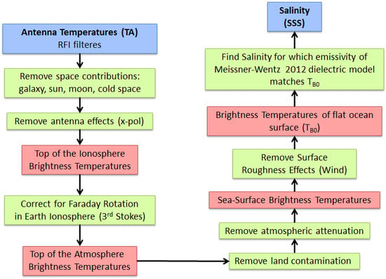
1. Introduction

NASA’s Aquarius mission [1] measured ocean surface salinity from late August 2011 until early June 2015. The end-of mission (Version 5) data release [2] in December 2017 provides an important legacy data set of ocean salinity for the oceanographic research community. It is the goal of this publication to highlight the most important aspects of the Aquarius Version 5 salinity retrieval algorithm. Many technical details of the algorithm are given in the Algorithm Theoretical Basis Document (ATBD) [3], to which the interested reader is referred. Here, we will focus on the parts of the Version 5 algorithm that have not yet been published. Another goal of our paper is to demonstrate the improvements in the Version 5 algorithm over prior releases [4]. Finally, we will show how the Aquarius Version 5 salinity retrieval algorithm can be adapted to the SMAP (Soil Moisture Active Passive) Mission [5,6]. SMAP has been measuring ocean surface salinity [7] since 1 April 2015 and thus is continuing the Aquarius legacy data.

Our paper is organized as follows: Section 2 gives a schematic overview of the steps in the salinity retrieval algorithm. It also contains a brief discussion of the necessary ancillary inputs and the concept of the expected antenna temperature, which is computed by a reference salinity field. We will then discuss various components of the algorithm: surface roughness correction (Section 3), atmospheric correction (Section 4), reflected galaxy correction (Section 5) and correction for side-lobe intrusion from land surfaces (Section 6). The ocean target calibration and calibration drift correction is the subject of Section 7. In Section 8 we discuss the various error sources and how formal estimates for the retrieval uncertainties can be obtained. Section 9 briefly summarizes the validation of the Aquarius Version 5 retrievals versus in-situ measurements from the ARGO network and exhibits how the Version 5 results have improved over prior versions. Finally, in Section 10 we discuss how the Aquarius Version 5 algorithm can be adapted to retrieving salinity with SMAP. Section 11 summarizes our main findings.

2. Major Steps of the Salinity Retrieval Algorithm

2.1. Basic Algorithm Flow

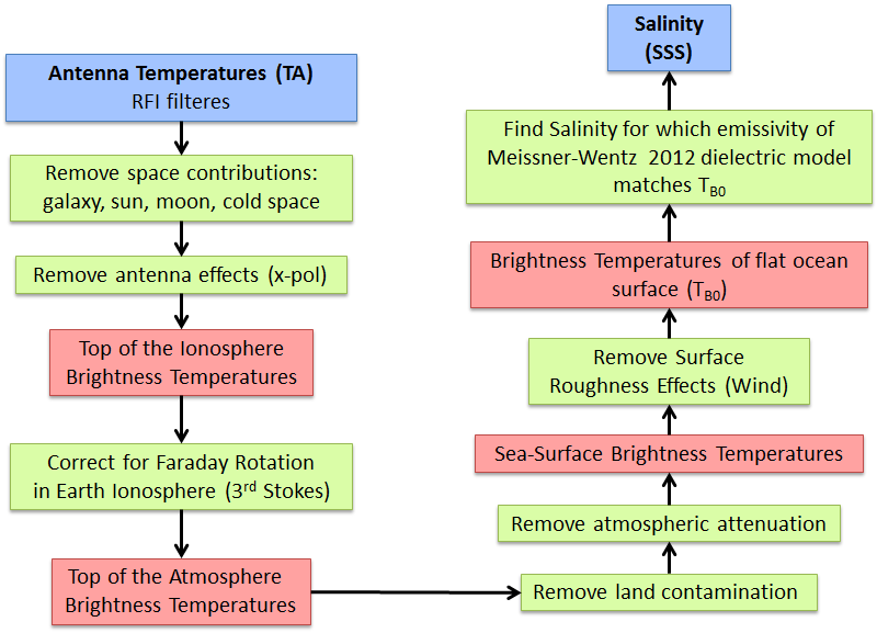
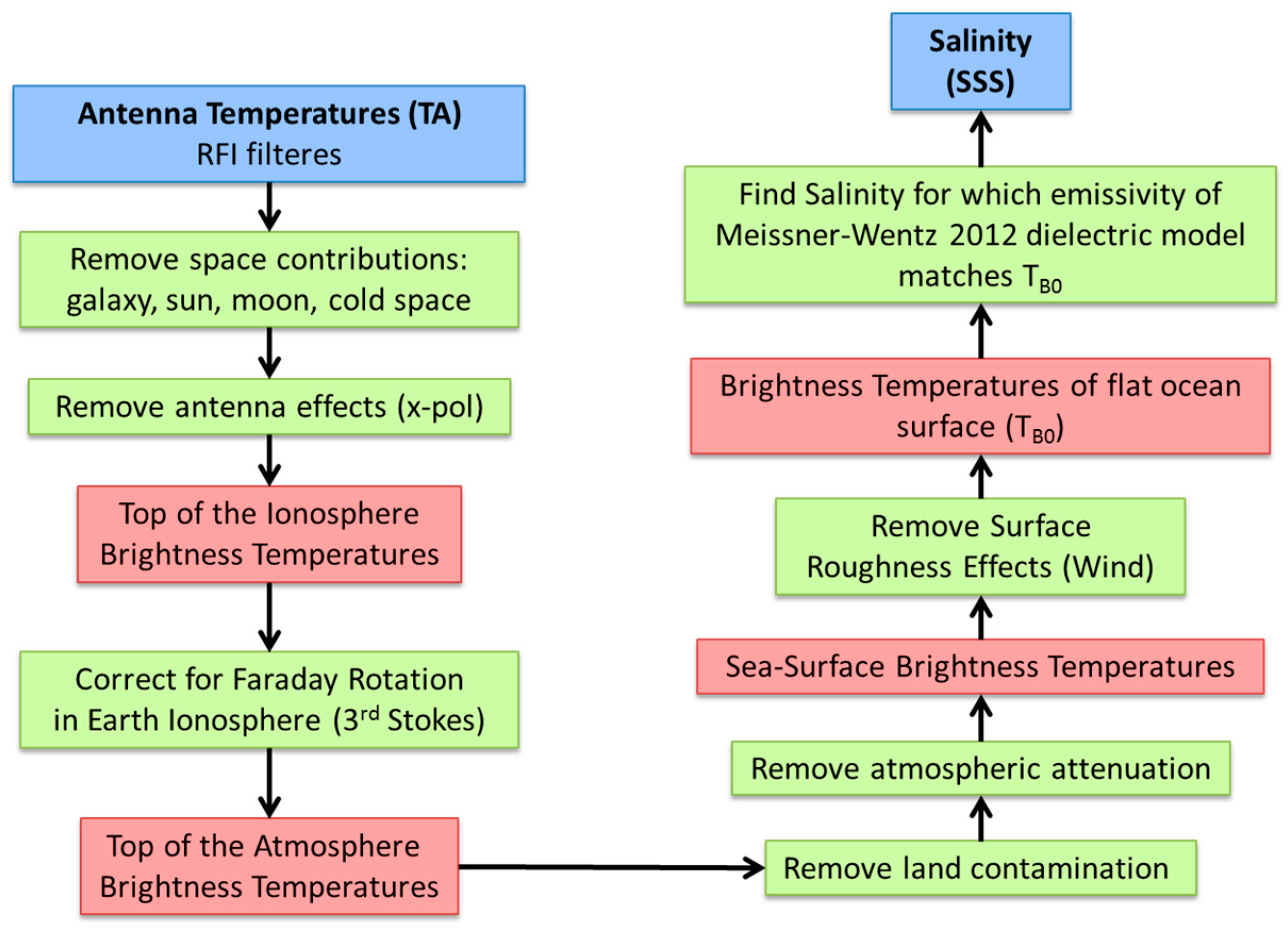
The basic inputs to the Aquarius Version 5 salinity retrieval algorithm are the antenna temperature (TA) measurements from the Aquarius radiometer, which have been filtered for radio frequency interference (RFI) [8,9], and radar backscatter (σ₀) measurements from the Aquarius scatterometer. The output is sea-surface salinity (SSS) and many intermediate variables required for the salinity calculation. The algorithm (Figure 1) consists of a number of steps that are intended to remove unwanted signals: radiation from galaxy, sun, moon and the cosmic microwave background (CMB), antenna cross-polarization contamination, Faraday rotation in the Earth’s ionosphere, attenuation in the Earth’s atmosphere and radiation from land surfaces. The result of these successive corrections is the brightness temperature (TB) that is emitted from the ocean surface. Finally, the effect of the wind roughening of the ocean surface is removed leading to the brightness temperature (T_B0) that is emitted from a flat ocean surface. A maximum likelihood estimator (MLE) is then used to estimate salinity from T_B0. The MLE minimizes the sum of square (SOS) difference between the Aquarius measurements of T_B0 of the two polarizations (vertical V and horizontal H) and the values of the radiative transfer model calculation for T_B0. This model calculation which is based on the dielectric constant of sea-water [10,11,12]. Figure 1 shows a schematic flow diagram of the salinity retrieval algorithm.

2.2. Ancillary Inputs

The salinity retrieval algorithm also requires a number of ancillary input fields. The most important ones are discussed in this section:

2.2.1. Sea Surface Temperature (SST)

SST is a crucial input to the dielectric constant model [10,11,12], which enters the computation of the emissivity of a flat ocean surface. An evaluation was made of the performance of the SSS retrieval algorithm with various ancillary SST fields [13]. The result of the analysis was that the best performance is obtained with the daily GHRSST (Gridded High-Resolution SST) Level 4 field from the Canadian Meteorological Center (CMC). It is gridded at 0.2° resolution and available from the PO.DAAC web site (https://podaac.jpl.nasa.gov/dataset/CMC0.2deg-CMC-L4GLOB-v2.0). Version 5.0 uses this ancillary SST field. The CMC field is linearly interpolated in space and time to the boresight location of the Aquarius observation.

2.2.2. Atmospheric Profiles

The atmospheric profiles for pressure, temperature, relative humidity, and cloud water mixing ratio are used in the correction for atmospheric absorption. They are obtained from the NCEP (national Centers for Environmental Prediction) GDAS (General Data Assimilation System) 1-deg 6-hourly fields are used, which are available from http://nomads.ncep.noaa.gov/. All fields are linearly interpolated in space and time to the boresight location of the Aquarius observation.

2.2.3. Wind Speed Background Field

The NCEP GDAS 1-deg, 6-h scalar wind speed field is used as background field in the Aquarius wind speed retrievals [12]. It is available from http://nomads.ncep.noaa.gov/. It is linearly interpolated in space and time to the boresight location of the Aquarius observation.

2.2.4. Wind Direction

The NCEP GDAS 1-deg, 6-h scalar wind direction field is used in the surface roughness correction and in the Aquarius wind speed retrievals [12]. It is available from http://nomads.ncep.noaa.gov/. It is linearly interpolated in space and time to the boresight location of the Aquarius observation.

2.2.5. Land Mask

We use the static 1-km land/water mask from the OCEAN DISCIPLINE PROCESSING SYSTEM (ODPS). It is based on World Vector Shoreline (WVS) database and World Data Bank and was provided as courtesy of Fred Patt, Goddard Space Flight Center, [email protected]. From the land mask two values of the land fraction are computed. The first one, called $f_{land}$, is defined as the fraction of land area within an antenna 3 dB footprint, where the land area consist of the sum of 1-km land pixels that fall within the footprint. A second land fraction, called $g_{land}$, is the fractional land area weighted by the antenna gain pattern, and the integration is taken over the whole Earth field of view. For details see ([3], page 34 + 35).

2.2.6. Rain Rate and Rain Flagging

The instantaneous rain rate (IRR) is used as a quality control indicator in the ocean target calibration (Section 7) and in the validation (Section 9) when matching Aquarius observations with in-situ salinity measurements from ARGO drifters. Aquarius measures ocean salinity within a few centimeters of the surface, whereas ARGO measures salinity at 5 m depth. In order to avoid mismatches between the two measurements resulting from salinity stratification within the upper ocean layer under precipitation [14], it is necessary to have information on rain rate, which is used to flag observations with rain. Our IRR, provided by the Aquarius Rain Accumulation (RA) product [15], is used as an ancillary data set that aids users of the V5.0 Aquarius Level 2 data to better understand the salinity stratification changes due to rain. The product uses as input the surface rain rates from the NOAA CMORPH (CPC-Climate Prediction Center-Morphing technique) global precipitation data set [16]. The average instantaneous rain rate is calculated using a structure of 13 CMORPH pixels around the center of the Aquarius IFOV, where the weight associated with each pixel is based on the antenna gain. We want to emphasize that an Aquarius observation that has been rain flagged according to this procedure is not to be regarded as degraded or bad. The surface rain freshening is a real signal that is picked up by the satellite but not by ARGO floats or models. The rain flag solely serves the purpose to indicate not to use this observation when validating Aquarius salinity measurements against ARGO drifters.

2.3. Forward Model and Expected TA

The forward model calculates the Aquarius TA, also called expected TA, for a given Earth scene by reversing the steps of the retrieval algorithm. The expected TA serves as an important diagnostic tool in the assessment of the geophysical model that is used in the salinity retrieval and also in the sensor calibration. The computation of TA expected requires an external reference salinity field as crucial input in the computation of T_B0 for a flat ocean surface. The reference salinity field for Aquarius Version 5 is the monthly 1-degree gridded interpolated ARGO SSS field provided by Scripps (http://www.argo.ucsd.edu/Gridded_fields.html). It is linearly interpolated in space and time to the boresight location of the Aquarius observation. At high latitudes (above 65 N/S) and very close to land where no ARGO data exist V5.0 uses the HYCOM salinity (www.hycom.org) as reference field, after linearly interpolating in space and time to the Aquarius observation. It should be noted that only the global average of the expected TA enter the salinity retrieval algorithm through the ocean target calibration (Section 7). Because of that, the Aquarius salinity retrieval algorithm uses effectively only the global 7-day average of the Scripps ARGO field.

3. Surface Roughness Correction

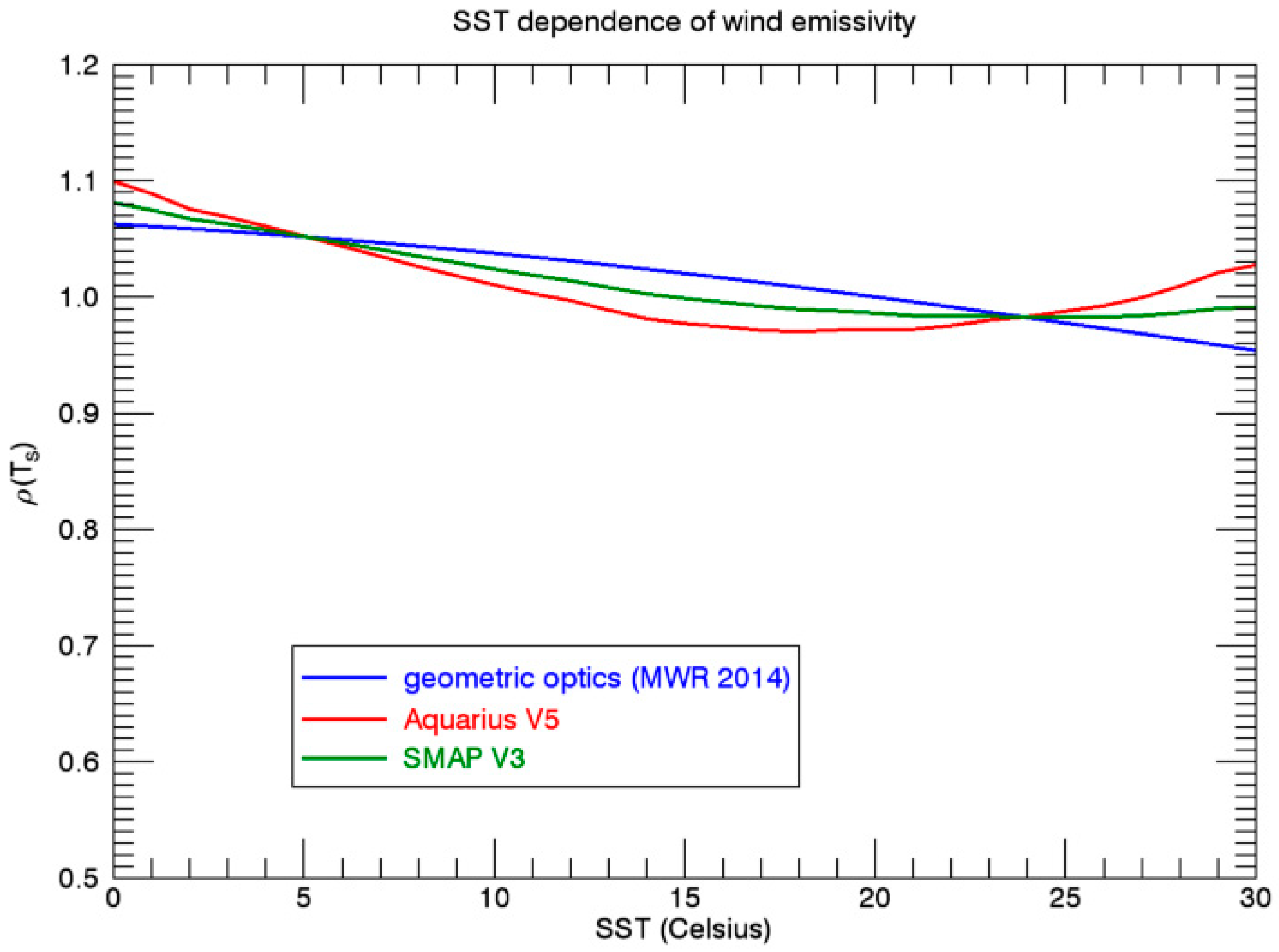
The correction of the wind induced surface roughness and the model for the wind induced emissivity in the Aquarius salinity retrieval algorithm is based on the results of [12]. In Version 5 a few changes were implemented. The purpose for these changes was the mitigation of biases that have been found in earlier releases and that could be traced back to the surface emissivity model. The major change from [12] concerns the SST dependence of the wind emissivity $\Delta E_W$. The functional form $\rho \left(T_S\right)$ of this SST dependence in Version 5, which is shown in Figure 2, is given as follows:

$$\begin{array}{l}\Delta E_W=\delta \left(W,{\phi }_r\right)\cdot \rho \left(T_S\right)\\ \rho \left(T_S\right)=\left[\frac{E_0\left(T_S\right)}{E_0\left(T_{ref}\right)}+{\rho }^{\prime }\left(T_S\right)\right],\end{array}$$

(1)

where $T_S$ denotes SST and $T_{ref}=20{}^{\mathrm{o}}\mathrm{C}$. The harmonic expansion $\delta \left(W,{\phi }_r\right)$ of the wind emissivity, which depends on the wind speed $W$ and wind direction, ${\phi }_r$ relative to the azimuthal look, is given in Equation (7) of [12]. The 1st term in the expression for $\rho \left(T_S\right)$ is the SST dependence that was used in [12]. It is proportional to the flat surface emissivity $E_0$. As explained in [11] it can be understood within the geometrics optics approach for the rough ocean surface by the fact that the wind roughened surface mixes the vertical and horizontal polarizations of the specular surface and the mixing increases with increasing emissivity of the specular surface. The additional term ${\rho }^{\prime }\left(T_S\right)$ is the empirically derived change that was made in the Version 5 algorithm.

4. Atmospheric Absoprtion Correction

4.1. Atmospheric Absoprtion and Correction Algorithm

The radiation that is emitted from the ocean surface is attenuated by the Earth’s atmosphere. The brightness temperature at the top of the atmosphere (TOA) is given by [3,11,17]:

$$T_{B,TOA}=T_{BU}+\tau \cdot \left(E\cdot T_S+T_{B\Omega }\right).$$

(2)

$T_{BU}$ is the brightness temperature of the upwelling atmospheric radiation, $\tau$ is the atmospheric transmittance, $E$ is the ocean surface emissivity, $T_S$ is the sea surface temperature and $T_{B\Omega }$ is the downwelling sky radiation that is scattered off the ocean surface in the direction of the observation. At L-band frequencies, it is a very good approximation to write [3]:

$$T_{B\Omega }=R\cdot \left(T_{BD}+\tau \cdot T_{B\cos }\right),$$

(3)

where $T_{BD}$ is the downwelling atmospheric radiation that is incident on the ocean surface, $T_{B\cos }$ is the cosmic microwave background radiation and $R=1-E$ is the ocean surface reflectivity.

The values for $\tau$, $T_{BU}$ and $T_{BD}$ are given as integrals over the vertical profiles atmospheric absorption coefficients [3,11,17]. At L-band frequencies the only significant sources of atmospheric attenuation are due absorption by oxygen, water vapor and cloud liquid water. The calculation of the atmospheric absorption coefficients requires the atmospheric profiles for pressure, temperature, relative humidity, and cloud water mixing ratio as ancillary input (see Section 2.2.2).

The atmospheric absorption correction in the salinity retrieval algorithm (Figure 1) inputs the TOA brightness temperatures $T_{B,TOA}$ and outputs ocean surface emissivities $E$ and the surface brightness temperatures $T_{B,SUR}=E\cdot T_S$ by inverting Equation (2) using (3).

4.2. Oxygen Absorption Model

The oxygen absorption is the largest constituent among the three sources of atmospheric attenuation at L-band. Its radiometric contribution to the total TOA TB amounts to a few Kelvin. At L-band frequencies, which are far from the oxygen absorption lines, the oxygen absorption is caused almost entirely by non-resonant continuum absorption, which is difficult to determine experimentally.

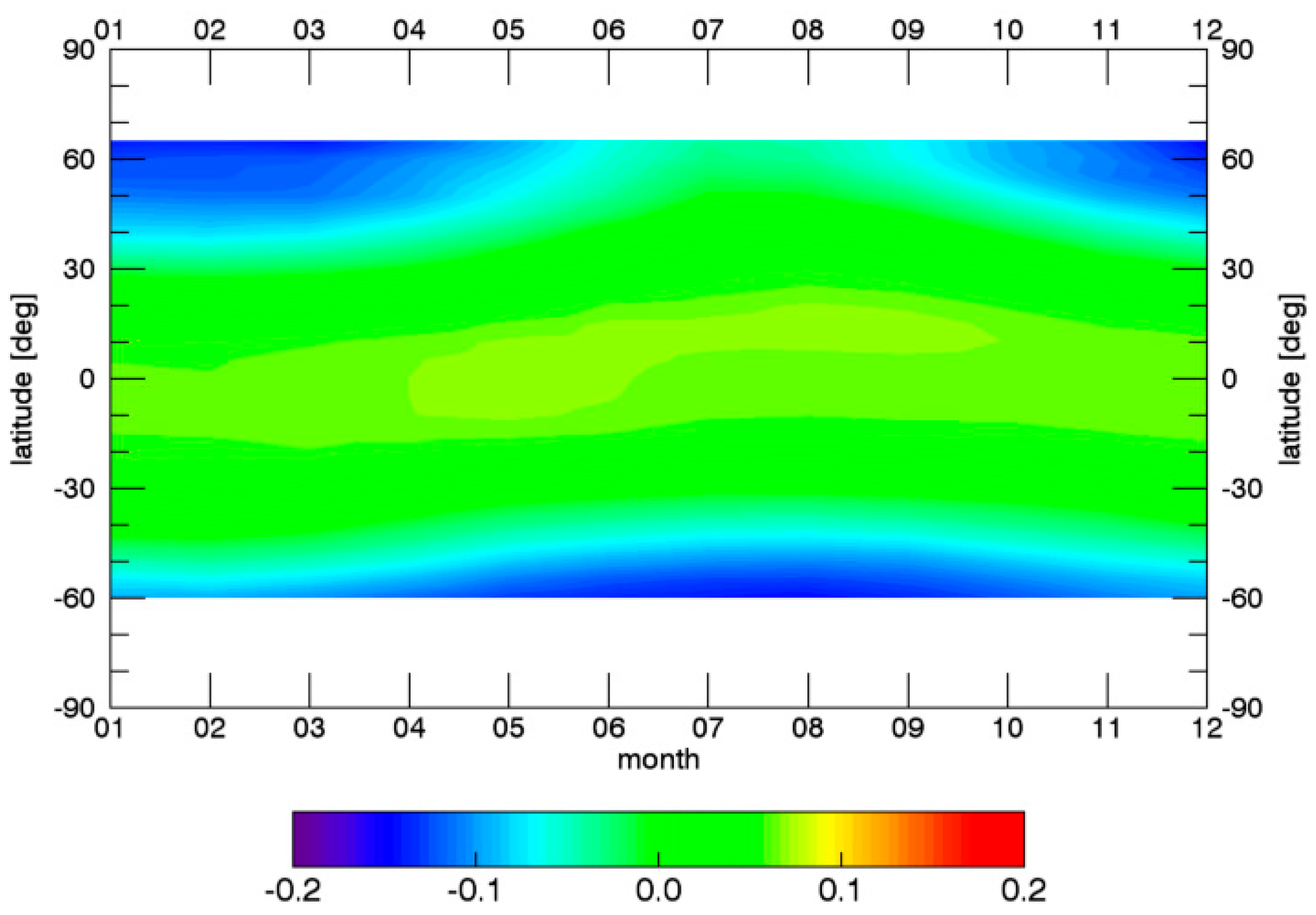
Prior to Version 5, all Aquarius salinity releases had used the oxygen absorption model of Wentz and Meissner [18], which has been extensively used in retrieval algorithms at higher frequencies. The salinity retrievals of these prior versions showed spurious seasonal salty biases at high N and S latitudes, which were largest the N Pacific during April and May. These biases have been tracked back to the oxygen absorption model. It has been found that these biases can be significantly reduced by reverting to the oxygen absorption model of Liebe et al. [19], which is based on laboratory measurements. The Version 5 algorithm uses the oxygen absorption model of [19]. The difference between the two oxygen absorption models is the dependence of the oxygen absorption coefficient of air temperature $T_{air}$. This temperature dependence is given by the expression ${\left(\raisebox{1ex}{$300K$}\!\left/ \!\raisebox{-1ex}{$T_{air}$}\right.\right)}^{\alpha }$. The numerical value of the exponent $\alpha$ is 1.5 in [18] and it is 0.8 in [19]. This means that the change of the absorption coefficient as function of air temperature when going from warm to cold temperatures has effectively been reduced in Version 5 by about 50% compared to prior versions. Figure 3 depicts the radiometric impact of the change in the O₂ absorption by showing the difference in the correction (TOA TB minus surface TB) between the two absorption models as function of time and latitude.

5. Reflected Galaxy Correction

Another large source of error that needs to be corrected in the salinity retrieval algorithm is the reflected radiation from the galaxy [20]. It can be large (5 Kelvin) and is difficult to deal with as it requires an accurate knowledge of the location and strengths of the galactic radiation, an analytic model for the wind induced roughness of the ocean surface and the antenna gain pattern.

5.1. Geometric Optics Model

For a flat ocean the contribution of the reflected galactic radiation to the antenna temperature $T_{A,gal,ref}$ is given by integrating radiation from the galactic sources and reflected at the ocean surface over the antenna gain pattern. Location and strength of the galactic sources at L-band are taken from the galactic map [20,21], which was derived from radio-astronomy observations. In actuality, bistatic scattering from a rough ocean will result in galactic radiation entering the mainlobe of the antenna from many different directions. In effect, a rough ocean surface tends to add additional spatial smoothing to $T_{A,gal,ref}$. Modeling of this effect is based on the geometric optics (GO) approach, in which the rough ocean surface is modeled as a collection of tilted facets, with each facet acting as an in-dependent specular reflector. The formulation for this model is given by [22] and the technical details of its application to calculating the TB of reflected galactic radiation at a rough ocean surface are spelled out in [3]. A crucial input to the GO model is the distribution of the slopes of the tilted facets of the rough ocean surface, which depends on wind speed $W$. The Aquarius algorithm uses the slope variance from [11]. At L-band frequencies this value represents about a 50% reduction in the slope variance from the classic Cox and Munk experiment [23], which measured the ocean sun glitter distribution.

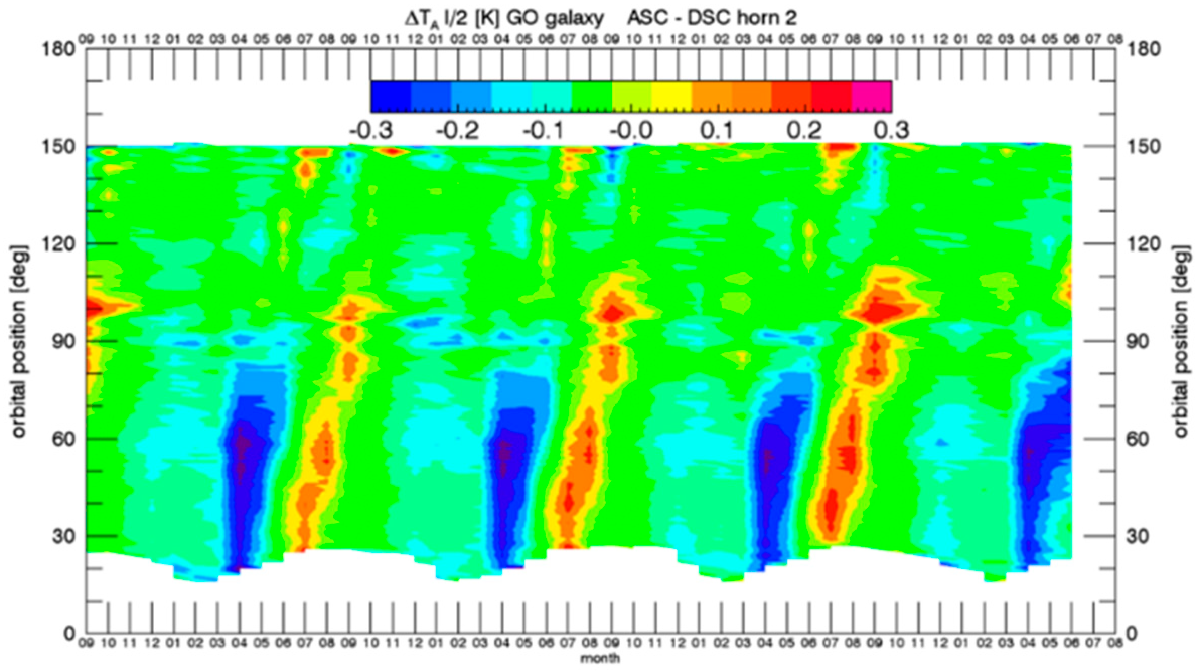
The accuracy of the GO model can be estimated by looking at the zonal differences between the morning (descending) and the evening (ascending) swaths over the same ocean (Figure 4) and comparing them with the size of the reflected galactic correction (not shown). Ideally, the differences between ascending and descending swaths should vanish when averaged over weekly to monthly time scales. From Figure 4, we conclude that the GO model removes the reflected galactic radiation correctly to about 90%. The remaining 10% shows up as spurious signal in the Aquarius salinity retrievals.

5.2. SMAP Fore—Aft Analysis

Observations from SMAP provide an opportunity to improve the correction for the reflected galactic signal. SMAP performs a full 360° scan in less than 5 s and thus observes each location in forward (fore) and backward (aft) direction within a couple minutes. The (relatively) strong reflected radiation emanating from the plane of the galaxy can appear in both the forward and the backward look but usually not at the same time. Radiation from directions other than the plane of the galaxy are generally quite small [20]. If all other signals that depend on look direction (Faraday rotation, wind direction, solar and lunar radiation) have been accurately removed [7], then taking the difference between fore and aft measured TA produces the reflected galactic radiation:

$$T_{A,gal,ref}\left({\varphi }_{fore}\right)-T_{A,gal,ref}\left({\varphi }_{aft}\right)=T_A\left({\varphi }_{fore}\right)-T_A\left({\varphi }_{aft}\right).$$

(4)

Here, $\varphi$ denotes the azimuthal look angle. This equation can be used to derive an empirical galactic correction separate for the SMAP fore and aft looks. For example, looking for cases where the signal from the aft look is small (<2 K) and assuming that the model (theory) for the SMAP aft look reflected galactic radiation is correct if it is smaller than 2 K, then the empirical correction for the fore look can then be obtained from (4) as:

$$T_{A,gal,ref,emp}\left({\varphi }_{fore}\right)=T_{A,meas}\left({\varphi }_{fore}\right)-T_{A,meas}\left({\varphi }_{aft}\right)+T_{A,gal,ref,model}\left({\varphi }_{aft}\right).$$

(5)

Likewise, assuming that the computed SMAP fore look galaxy model is correct if it is smaller than 2 K, then the empirical galaxy model for the aft look can then be obtained from (4) as:

$$T_{A,gal,ref,emp}\left({\varphi }_{aft}\right)=T_{A,meas}\left({\varphi }_{aft}\right)-T_{A,meas}\left({\varphi }_{fore}\right)+T_{A,gal,ref,model}\left({\varphi }_{fore}\right).$$

(6)

When performing the analysis, observations were discarded for which the reflected solar radiation is not negligible. Reflected solar radiation differs between fore and aft looks and currently the correction for reflected solar radiation in the SMAP algorithm is not accurate enough to correct for the difference. It is possible to find observations for all times and orbit positions for which both the reflected solar radiation is negligible and either the TA galaxy of the fore or the aft look are less than 2 K. Therefore, it is possible to derive empirical galactic corrections with the SMAP sensor for both look directions using Equations (5) and (6). Separate derivations are performed for different wind speed regimes using 5 m/s intervals.

The largest part of the SMAP fore—aft results can be reproduced using a tilted facet calculation as explained in Section 5.1 but adding 2 m/s to the wind speed when calculating the RMS slope variance. The effective increase in slope variance increases the surface roughness at L-band frequencies and this increase brings the slope variance from the value in Section 5.1 closer to the Cox-Munk value [23].

Based on the prescription to add 2 m/s to the wind speed when deriving the reflected galactic correction from the geometric optics calculation (Section 5.1) a revised correction for the reflected galaxy for Aquarius can be derived, which takes the results from the SMAP fore—aft analysis into account [3].

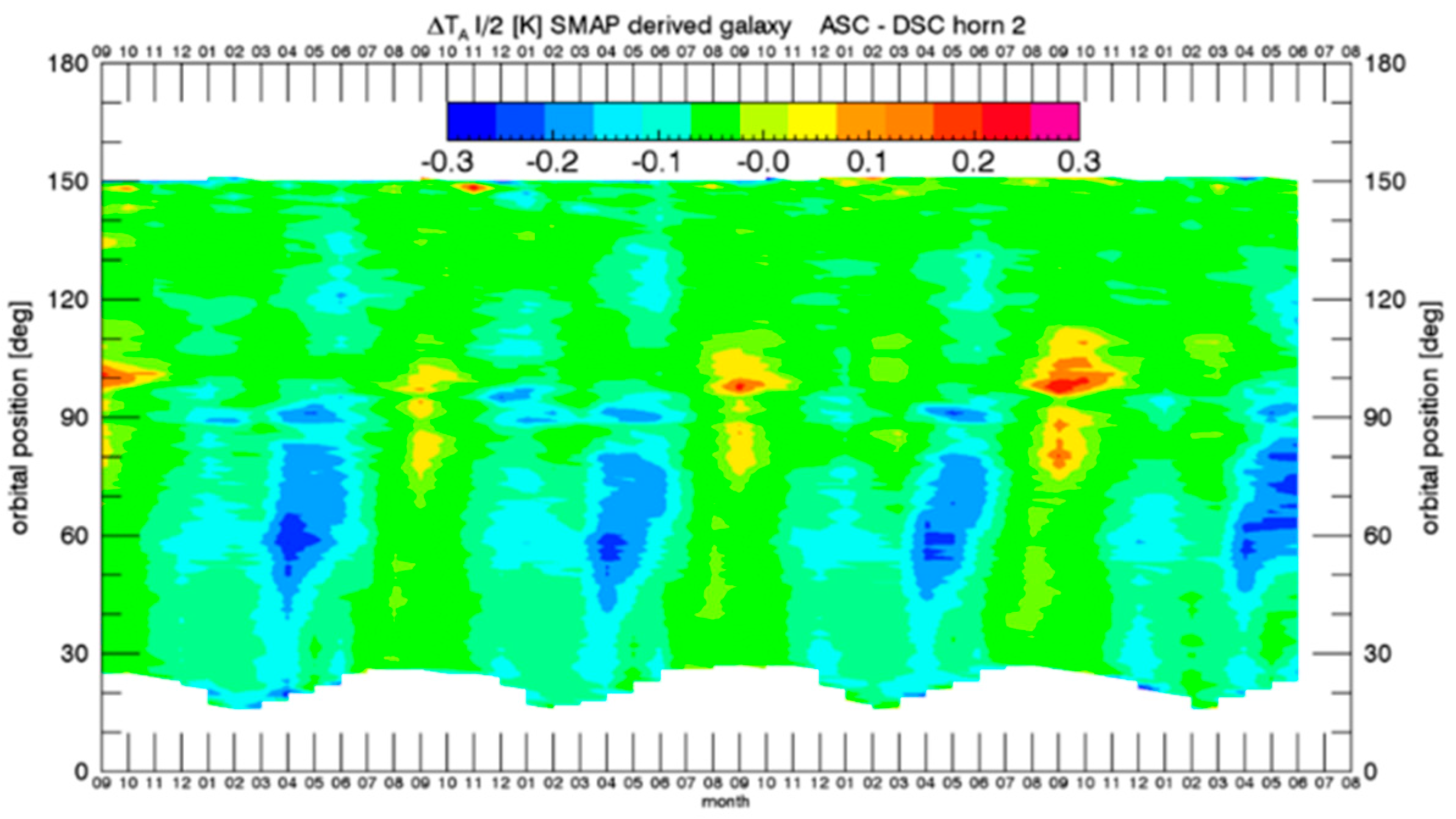
Figure 5 shows the significant improvement in the biases between ascending (evening) and descending (morning) swaths when using the SMAP fore—aft result compared with the original geometric optics calculation (Figure 4). However, Figure 5 also shows that even with this improvement in the galactic reflected model based on SMAP, some residual ascending—descending biases still remain, which would cause unacceptably large inaccuracies in the retrieved Aquarius salinity. Mitigating these residual ascending—descending biases is the goal of the empirical zonal symmetrization correction, which is the subject of the following section.

5.3. Emprirical Zonal Symmetrization

There are several possible reasons for the remaining inaccuracies in the reflected galaxy correction:

• The value of the variance of the slope distribution is not completely correct, even after effectively increasing the roughness by adding 2 m/s to the wind speed based on the SMAP fore—aft results.
• Errors in the antenna gain patterns used to derive the tables of the GO model.
• Other ocean roughness effects, which cause reflection of galactic radiation but cannot be modeled with an ensemble of tilted facets (e.g., Bragg scattering at short waves, breaking waves and/or foam, and net directional roughness features on a large scale).

The galactic tables themselves, which were derived from radio astronomy measurements [20,21]. For example, there is a small polarized component and Cassiopeia A is very strong and variable.

Such effects are very difficult or impossible to model. We have therefore decided to derive and use an empirical correction for the reflected galactic radiation, which is added to the GO calculation. The danger in doing this is that other geophysical issue (i.e., not associated with reflected radiation from the galaxy) could be masked. But, it was decided to accept this risk for V5.0.

This empirical correction is based on symmetrizing the ascending and the descending Aquarius swaths. The basic assumptions are:

• There are no zonal ascending—descending biases in ocean salinity on weekly or larger time scales.
• The residual zonal ascending—descending biases that are observed are all due to the inadequacies (either over or under correction) in the GO model calculation for the reflected galactic radiation.
• The size of the residual ascending—descending biases is proportional to the strength of the reflected galactic radiation.

Assumption A is based on current understanding of the structure of the salinity field for which there no known physical processes that would cause such a difference. Assumption B results from analyses of the salinity fields and known limitation of the GO model. Assumption C is based on theory for scattering from rough surfaces and the assumption that the source of any difference is reflected galactic radiation and the fact that the source and surface are independent. It is expected to hold in some mean sense over the footprint.

A symmetrization of the ascending and descending Aquarius swaths can be done on the basis of a zonal average. According to Assumption C above the symmetrization weights will be determined by the strength of the reflected galactic radiation. We describe the symmetrization procedure for the 1st Stokes parameter, which is the sum of the brightness temperatures at the ocean surface and will be denoted by $T_B$. In the equations below, $\langle \dots \rangle$ denotes the zonal average and the variable $z$ denotes the orbital angle (z-angle). If $z$ lies in the ascending swath, then $-z$ (or ${360}^{°}-z$) lies in the descending swath and vice versa. $T_B\left(z\right)$ is first Stokes parameter as measured by Aquarius at the surface at $z$. $T_{A,gal,ref}\left(z\right)$ is the value of the reflected galactic radiation received by Aquarius as computed based on the SMAP fore—aft results (Section 5.2). The symmetrization term, $\Delta \left(z\right)$, which is the basis of the empirical correction, is given as:

$$\begin{array}{c}\Delta \left(z\right)=\left[p\cdot \langle T_B\left(z\right)\rangle +q\cdot \langle T_B\left(-z\right)\rangle \right]-\langle T_B\left(z\right)\rangle \\ p=\frac{\langle T_{A,gal,ref}\left(-z\right)\rangle }{\langle T_{A,gal,ref}\left(z\right)\rangle +\langle T_{A,gal,ref}\left(-z\right)\rangle }\\ q=\frac{\langle T_{A,gal,ref}\left(z\right)\rangle }{\langle T_{A,gal,ref}\left(z\right)\rangle +\langle T_{A,gal,ref}\left(-z\right)\rangle }.\end{array}$$

(7)

The probabilistic channel weights $p$ and $q$ add up to 1: $p+q=1$. The symmetrized surface brightness temperature, called $T_B^{\prime }$, is given by:

$$T_B^{\prime }\left(z\right)=T_B\left(z\right)+\Delta \left(z\right).$$

(8)

It is not difficult to see that this symmetrization has the following features:

• Assume that $z$ lies in the ascending swath and therefore $-z$ lies in the descending swath. If there is no reflected galactic radiation in the ascending swath, i.e., $\langle T_{A,gal.ref}\left(z\right)\rangle =0$, then $p=1$ and $q=0$. That means that the symmetrization term and thus the whole empirical correction $\Delta \left(z\right)$ vanishes, and therefore: $T_B^{\prime }\left(z\right)=T_B\left(z\right)$.
• If, on the other hand, there is no reflected galactic radiation in the descending swath, i.e., $\langle T_{A,gal.ref}\left(-z\right)\rangle =0$, then $p=0$ and $q=1$. That implies $\Delta \left(z\right)=\langle T_B\left(-z\right)\rangle -\langle T_B\left(z\right)\rangle$ and thus $\langle T_B^{\prime }\left(z\right)\rangle =\langle T_B\left(-z\right)\rangle$.
• The zonal average of $T_B^{\prime }$ is symmetric: $\langle T_B^{\prime }\left(z\right)\rangle =\langle T_B^{\prime }\left(-z\right)\rangle$.
• If the reflected galactic radiation is the same in ascending and descending swaths $\langle T_{A,gal.ref}\left(z\right)\rangle =\langle T_{A,gal.ref}\left(-z\right)\rangle$, then $p=q=\frac{1}{2}$ and thus the global average (sum of ascending and descending swaths) does not change after adding the symmetrization term: $\langle T_B{}^{\prime }\left(z\right)\rangle +\langle T_B^{\prime }\left(-z\right)\rangle =\langle T_B\left(z\right)\rangle +\langle T_B\left(-z\right)\rangle$.
• If the zonal $T_B$ averages are already symmetric $\langle T_B\left(z\right)\rangle =\langle T_B\left(-z\right)\rangle$, then the symmetrization term and thus the whole empirical correction $\Delta \left(z\right)$ vanishes, and therefore: $T_B^{\prime }\left(z\right)=T_B\left(z\right)$. That means that our method will not introduce any additional ascending—descending biases that were not already there.

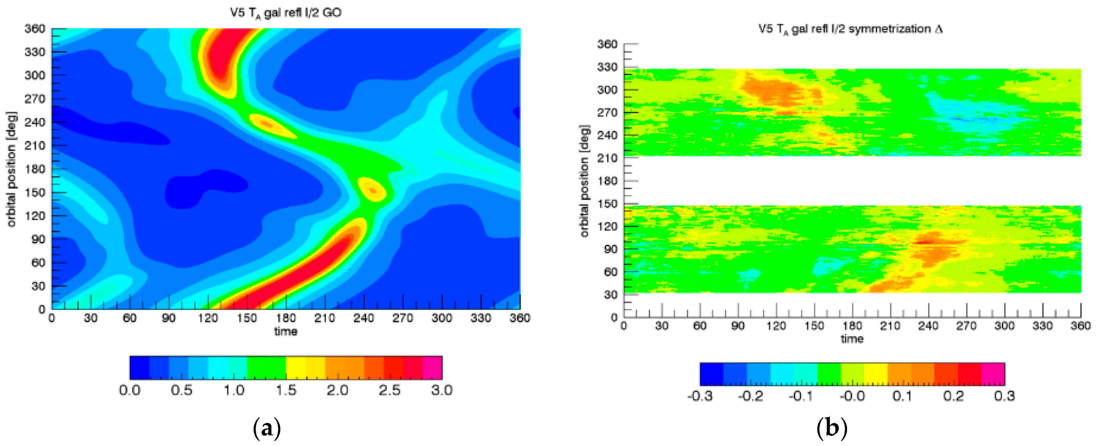
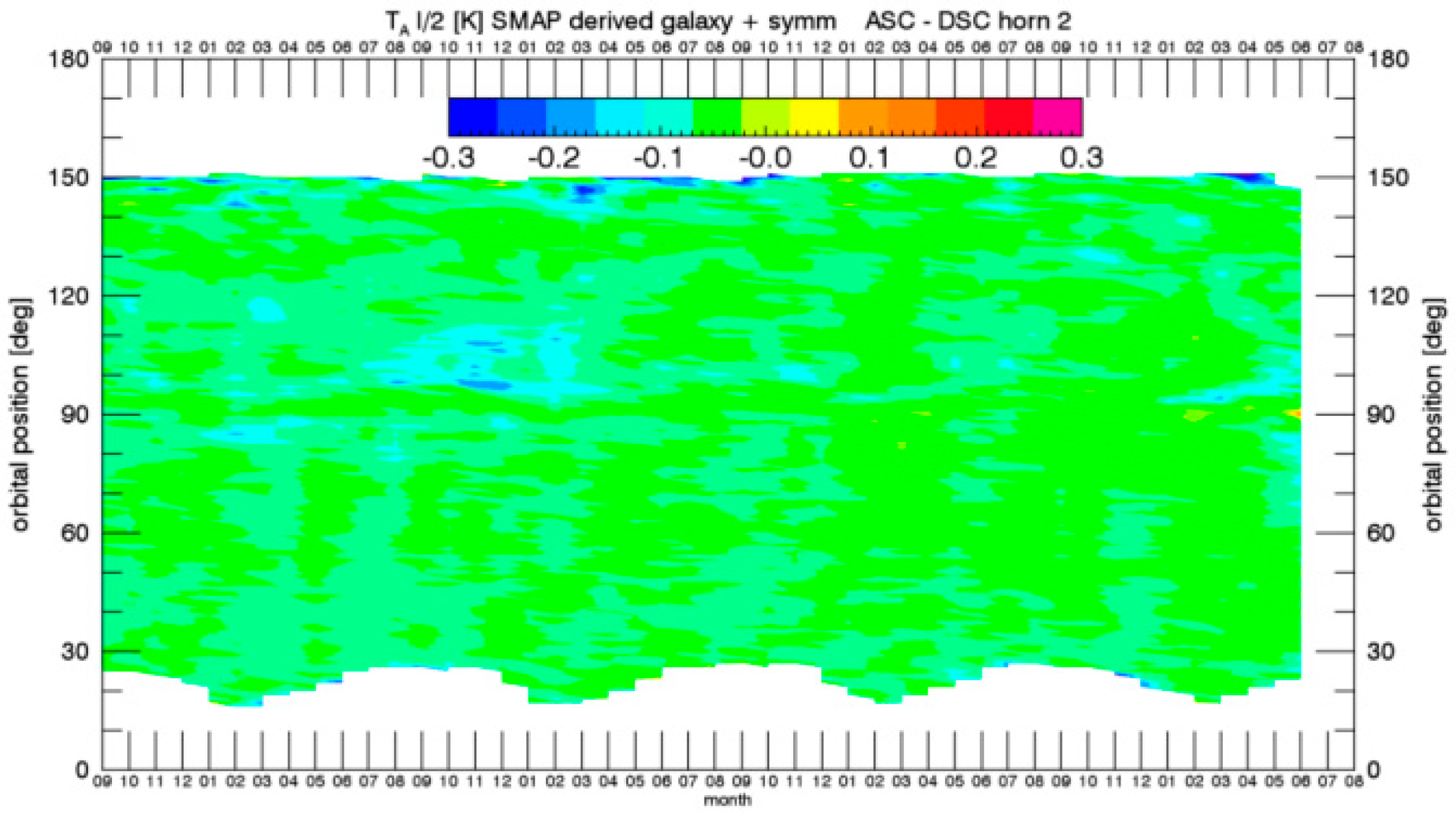
Figure 6 shows the size and pattern of the empirically derived symmetrization $\Delta$ in relation to the value of $T_{A,gal,ref}$ from the GO in time—z-angle space. For the GO computation we have assumed an average wind speed of 7.5 m/s. Sizeable contributions for $\Delta$ are observed in the vicinity of the galactic pattern that is obtained from the GO model. The magnitude of the peak values of $\Delta$ is about 0.2 K compared to about 3 K in $T_{A,gal,ref}$ from the GO model.

An important feature of this symmetrization procedure is the fact that it is derived from Aquarius measurements only and does not rely on or need any auxiliary salinity reference fields such as ARGO or HYCOM.

It is assumed that the galactic radiation itself is unpolarized and polarization occurs only through the reflection at the ocean surface. Ignoring Faraday rotation of the galactic radiation in the empirical correction term, its 2nd (Q) and 3rd Stokes (U) components are:

$${\Delta }_Q\approx \frac{R_V-R_H}{R_V+R_H}\cdot {\Delta }_I\approx \frac{T_{A,gal,ref,Q}}{T_{A,gal,ref,I}}\cdot {\Delta }_I,{\Delta }_U\approx 0,$$

(9)

where $R_{V,H}$ are the reflectivity for V and H polarization of an ideal (i.e., flat) surface.

Figure 7 shows the final ascending—descending biases after including the empirical zonal symmetrization. It is evident that all residual zonal biases have been effectively removed. That means, the empirical zonal symmetrization procedure is working as designed.

6. Correction for Sidelobe Intrusion from Land Surfaces

The Aquarius salinity retrievals degrade quickly as the footprint approaches land closer than 400 km. This land-contamination error occurs because the land is much warmer than the ocean. A correction for land entering the antenna sidelobes when the Aquarius observation gets close to land can be derived from simulated Aquarius brightness temperatures [3].

The land contamination is most conveniently dealt with the TOA (top of the atmosphere) (Figure 1). The error due to land contamination is given as:

$$\Delta T_{B,TOA}={\widehat{T}}_{B,TOA}-{\overline{T}}_{B,TOA,ml}.$$

(10)

The 1st term on the right hand side of (10) is the observed (i.e., measured) signal, which is computed from simulated TOA Earth brightness temperatures containing representative ocean and land scenes and integrating over the antenna gain patterns of the 3 Aquarius feedhorns. The 2nd term of the right hand side of (10) is the true TOA TB coming from the antenna main beam. Using the simulated Aquarius TB a table of the $\Delta T_{B,TOA}$ is computed one time off-line before the algorithm is run. This table is stratified according to the spacecraft nadir longitude (2881 elements in 0.125° increments), the spacecraft position in orbit (i.e., z-angle) (2881 elements in 0.125° increments), month (12 elements), polarization (V-pol, H-pol), and horn (inner, middle, and outer). When running the Aquarius salinity retrieval algorithm the value of $\Delta T_{B,TOA}$ is found by linearly interpolating the table to the exact spacecraft position. The interpolated value of $\Delta T_{B,TOA}$ is then subtracted from the actual TOA TB and then the retrieval process proceeds as outlined in Figure 1. The 3rd dimension of month is required to account for seasonal variability in the land brightness temperatures, although this effect is fairly minor. In order to calculate the true (i.e., theoretical) TB of the land surface we use a static monthly climatology of soil moisture and land surface temperatures that has been computed from NCEP fields (http://nomads.ncep.noaa.gov/.)

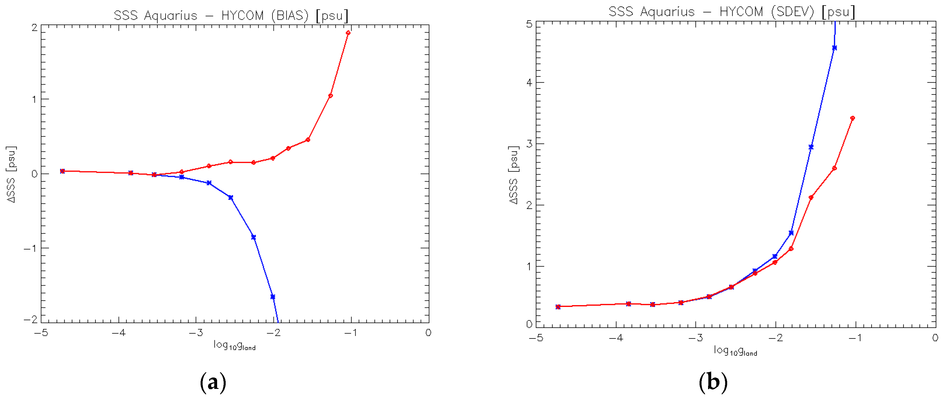
Figure 8 demonstrates the improvement in the salinity retrievals that is achieved by including the land correction. It shows bias (a) and standard deviation (b) between Aquarius and HYCOM salinity as function of the gain weighted land fraction $g_{land}$ (Section 2.2.5).

Even with the sidelobe correction for intrusion from land surfaces, the salinity retrieval algorithm degrades if the observation is too close to the coast. Figure 8a suggests that observations should be flagged if the value of $g_{land}$ exceeds 1%. We want to mention that the salinity retrieval algorithm does not attempt to correct for or flag freshwater plumes or discharges of rivers into the ocean. In contrast to the spurious signal caused by contamination from land surfaces, the river discharge is a real signal that is picked up by the satellite. It might not be picked up correctly by the models (HYCOM) or by the ARGO drifters, as the drifters cannot be deployed close to the continental shelf. Therefore, the Aquarius salinity measurements can provide valuable information in these cases.

7. Ocean Target Calibration and Calibration Drift Correction

The Aquarius radiometer uses a reference load and noise diode injection as internal calibration targets [24] when converting radiometer counts to TA. The calibration is performed at each Level 2 report interval, which lasts 1.44 s. Unfortunately, the accuracy of the pre-launch values for the noise diode injection temperatures $T_{ND}$ are not sufficient for retrieving salinity. Moreover, immediately after launch it became evident that the values of $T_{ND}$ were drifting (probably outgassing) by several Kelvin, and also other components of the instrument change over time. It is therefore necessary to have a stable and well-known calibration target over long time scales (weekly—monthly) for determining the value of $T_{ND}$ and its time dependence. The global average of the ocean was adopted for this purpose.

The ocean target calibration uses a 7-day (103 orbit) running TA average, denoted by ${\langle \dots \rangle }_{OT}$ over the global ocean as calibration target. The goal of the calibration is to tune the calibration parameters, essentially gain and offset, so that for each Aquarius channel:

$${\langle T_{A,cal}-T_{A,\exp }\rangle }_{OT}=0.$$

(11)

$T_{A,cal}$ are the Aquarius TA measurements after the calibration adjustments are performed. $T_{A,\exp }$ are the expected TA and calculated as described in Section 2.3. The crucial input in this calculation is the reference salinity field, which is taken from Scripps ARGO (Section 2.3). That means essentially that the ocean target calibration forces the retrieved Aquarius salinity to the Scripps ARGO reference salinity on a global 7-day average. Note that only the global 7-day average of the Scripps ARGO field is used in the ocean target calibration. A consequence of this constraint is that it is not possible to make an independent prediction of the global salinity average from Aquarius, as its value is forced to agree with the one from Scripps ARGO. The average (11) is calculated for each orbit. The 7-day averaging window is chosen, because the Aquarius orbit repeat cycle is 7 days.

It is crucial that both the measured and expected TA in the average ${\langle \dots \rangle }_{OT}$ of the ocean target calibration, which determine the instrument calibration parameters, are of the highest possible quality and as much as possible free of errors. Therefore, a number of additional quality control checks, more rigorous than for the regular SSS product, are applied when calculating this average [3].

Equation (11) was used during the first week of Aquarius operations to adjust the prelaunch calibration of radiometers (i.e., gain and bias). The gain was tuned by adjusting the values of the reference noise diodes $T_{ND,0}$. As the mission progressed, it was apparent that the Aquarius calibration changes over time and therefore it is necessary to update the values for the noise diode $T_{ND}$ from these initial values. Two major drift components have been identified and analyzed, which have different time scales and different origins.

The first one is a transient gain drift, most likely caused by out-gassing of the noise diodes. It is slowly varying and decreasing with time with a total change over the mission on the order of one Kelvin. It varies by channel (horn and polarization). It is well modeled as an exponential time dependence of $T_{ND}$:

$$T_{ND}\left(n_{orbit}\right)=T_{ND,0}\cdot \left(1-c\right)c=A-B\cdot \exp \left(-D\cdot n_{orbit}\right)$$

(12)

where $n_{orbit}$ denotes the orbit number. The coefficients $A$, $B$ and $D$ in this exponential fit (12) are determined once using the time series of Aquarius measurements over the entire mission using the ocean target calibration condition (11). The updated values for $T_{ND}$ from (12) are used when converting radiometer counts to TA.

The second type calibration drift manifests itself in pseudo-periodic oscillations in $T_{A,meas}-T_{A,\exp }$, which appear to be superimposed on the exponential drift and occur on the time scales of weeks—months. Its magnitude is in the order a few tenth of a Kelvin and it varies with channel. The oscillations are termed “pseudo” because the calibration anomaly is not periodic in nature and only has a rough appearance of periodicity. One of the root causes for this oscillation was determined to be a locking issue in the backend Voltage to Frequency Converter (VFC), which impacts all counts of the radiometer including the reference calibration load. A correction for the pseudo-periodic oscillations (“wiggles”) has been developed and implemented that uses a hardware-based model that only requires inputs from the Aquarius radiometer and does not depend on the ocean or an external salinity reference field [25]. However, this correction scheme does not remove the “wiggles” completely and it is necessary to remove the residual to achieve the very high level of accuracy necessary for retrieving ocean salinity. An analysis of cold space maneuvers showed similar oscillations in several channels [26]. This indicates that these residual oscillations are not predominantly caused by the errors in the geophysical model used in the salinity retrievals but are likely an instrument issue whose root cause is currently not known. Therefore, it is warranted to remove them empirically in the instrument calibration process. It was decided for the Version 5 to treat this residual as an offset and to use the ocean target calibration (11) to remove them In order to remove the residuals, an offset correction is performed at each orbit to obtain the final calibrated TA:

$$T_{A,cal}={\tilde{T}}_A-{\langle {\tilde{T}}_A-T_{A.,\exp }\rangle }_{OT}.$$

(13)

Here, ${\tilde{T}}_A$ denotes the antenna temperature that is obtained after the exponential drift correction has been applied and the average is over 7 days. It is estimated that the residuals are removed to a level of about 0.01 K.

8. Error Sources and Formal Uncertainty Estimation

8.1. Methodology

Each Level 2 (L2) and Level 3 (L3) Aquarius Version 5 salinity retrieval [22] is associated with a formal uncertainty value [3,27,28]. In this section we present a method for formally assessing random and systematic uncertainties in the Aquarius salinity retrievals. The method is based on performing multiple retrievals by perturbing the various inputs to the retrieval algorithm and calculating the sensitivity of the Aquarius salinity to these inputs. Together with an error model for the uncertainties in the input parameters it is possible to calculate the uncertainty in the retrieved salinity.

The basic approach to formally assess an uncertainty of the Aquarius salinity retrieval $S\left(x_i,\dots \right)$ to a parameter $x_i$, for example wind speed, is to calculate the sensitivity of $S$ to $x_i$. This is done by running the Version 5 Aquarius L2 algorithm after perturbing the input $x_{i0}$ by a small amount $\pm \Delta x_i$. Assuming that we have an uncertainty estimate $\Delta x_i\left(x_{i0}\right)$ for the input parameter $x_{i0}$, then the corresponding uncertainty in $S$ is given by:

$$\Delta S_i\left(x_{i0}\right)\approx \frac{\partial S}{\partial x_i}\left(x_{i0}\right)\cdot \Delta x_i\approx \frac{S\left(x_{i0}+\Delta x_i\right)-S\left(x_{i0}-\Delta x_i\right)}{2\cdot \Delta x_i}\cdot \Delta x_i.$$

(14)

The assessment of the uncertainty in $S$ consists therefore in two parts:

• The computational/algorithm part, i.e., running each retrieval algorithm with the perturbed parameter values.
• Obtaining a realistic error model for all the uncertainties that are involved. This part is done offline and its results are fed into the perturbed retrievals.

When running the algorithm for a perturbed variable, all the other variables are left unperturbed. Performing the uncertainty estimation this way takes into account that a given uncertainty in one of the input parameter can translate to very different uncertainties in the retrieved salinity depending on the environmental scene. For example, the same error in the input wind speed that is used in the surface roughness correction or in the reflected galactic radiation will result in a much larger uncertainty in salinity in cold water where the sensitivity of the $T_B$ to salinity is low than it would in warm water where the sensitivity is higher. The SST of the scene is a major driver in the size of the salinity uncertainty.

It is necessary to separate the uncertainty $\Delta x_i$ in each input $x_{i0}$ into a random and a systematic component. As a general guideline:

• Uncertainties that fluctuate on larger time and spatial scales (1 month, >100 km) are treated as systematic uncertainties.
• Uncertainties that fluctuate on shorter time and length scales are treated as random uncertainties.

The distinction between random and systematic uncertainties becomes important when propagating the uncertainties from the 1.44 s measurement (L2) to the monthly or weekly L3 averages [2]. Whereas the random components are suppressed by a factor $1/\sqrt{N}$ when averaged over $N$ samples, the systematic components are simply the average of the individual uncertainties.

8.2. Error Sources

This section briefly discusses the major error sources of the Aquarius Version 5 salinity retrieval algorithm and the quantitative assessment of their uncertainty. Further details can be found in [3,27,28].

8.2.1. NEDT

The radiometer noise (NEDT) is approximately the standard deviation of the noise in each 10 ms sample. The effective noise for salinity retrieval is the noise in the basic 1.44 s Aquarius data block used in processing. This effective NEDT is computed as the standard deviation of the RFI filtered antenna temperatures (TF) in each 1.44 s cycle divided by the square root of the number of measurements within that data block. This error (effective NEDT) is treated as random. We compute the effective NEDT and the resulting error in the salinity for all 3 channels: V-pol, H-pol and the 3rd Stokes parameter. It is assumed that these 3 components are independent and that the resulting errors in the salinity can be added as root sum squares.

8.2.2. Wind Speed

The uncertainty in the Aquarius HHH wind speed, which is used in the surface roughness correction [3,12] can be estimated by comparing the Aquarius HHH wind speed with other wind speed sources, for example WindSat [29]. This uncertainty has both a random and a systematic component.

8.2.3. Wind Direction

For the uncertainty in the auxiliary NCEP wind direction field (Section 2.2.4) we assume 10° and treat it as random error. This value is suggested by comparing the NCEP wind direction with measurements from buoys [30] or satellites [31], for example QuikSCAT or WindSat.

8.2.4. SST

An estimate of the uncertainty in the ancillary SST input from CMC (Section 2.2.1) can be obtained by comparing the CMC SST field with other SST sources, for example from WindSat [29].

8.2.5. Reflected Galaxy

The estimated uncertainty in the correction for the reflected galactic radiation are treated as systematic and based on the bias of $T_{A,meas}-T_{A,\exp }$ as a function of $T_{A,gal,ref}$ and the Aquarius HHH wind speed. It is assumed that $T_{A,meas}-T_{A,\exp }$ characterizes the degradation of the salinity retrievals.

8.2.6. Land Contamination

The estimated uncertainty due to intrusion of radiation from land and sea ice surfaces into the sidelobes of the Aquarius antenna is treated as systematic and its estimation is based on the RMS of $T_{A,meas}-T_{A,\exp }$ as a function of the gain-weighted land fraction $g_{land}$.

8.2.7. Undetected RFI

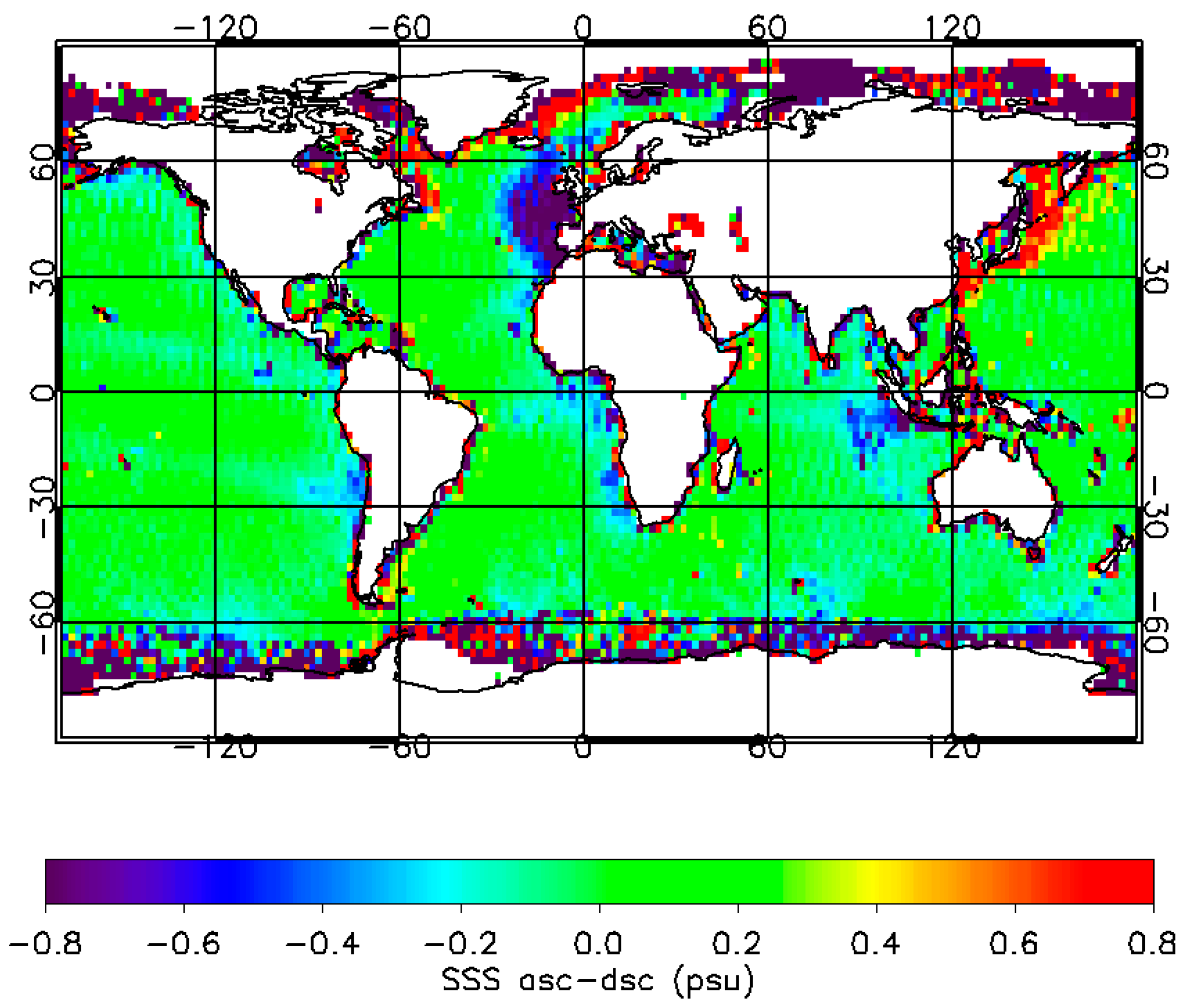
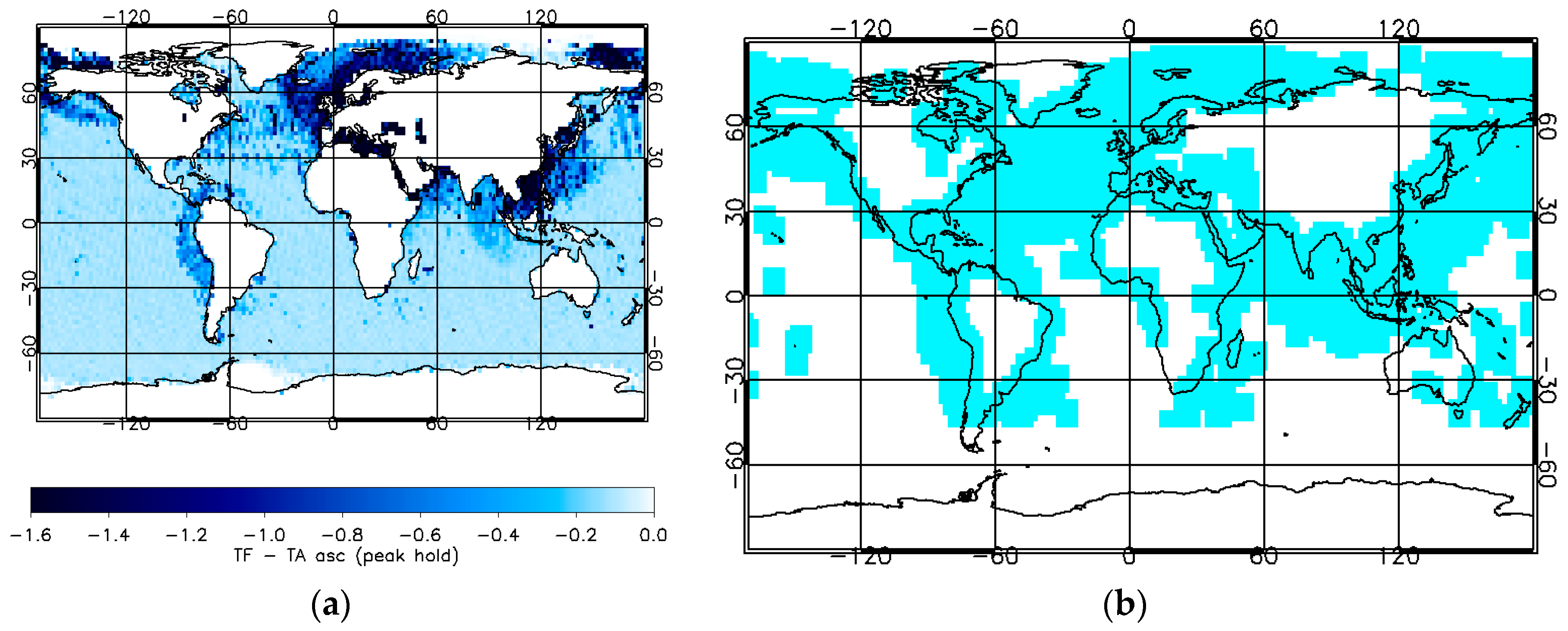
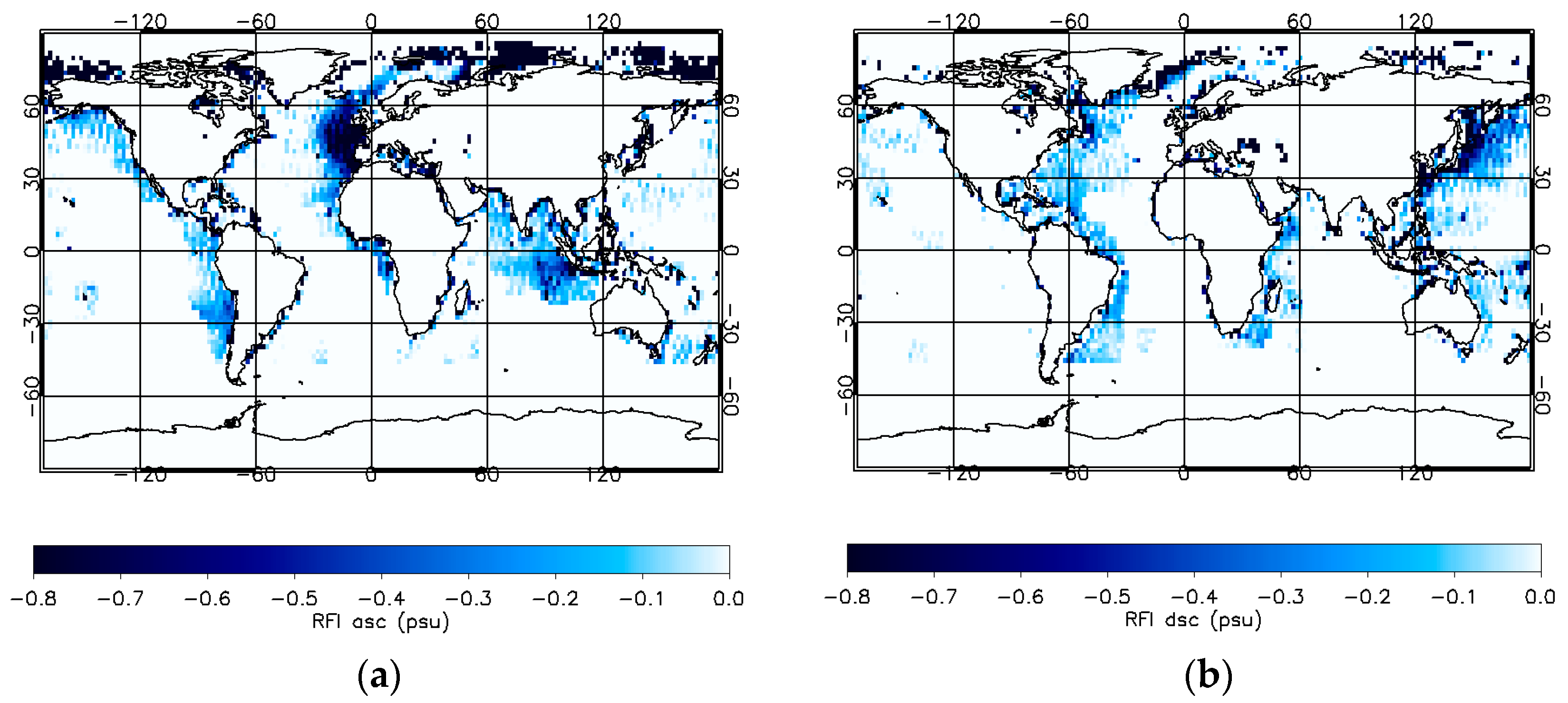
The signal from the Aquarius instrument is filtered for radio-frequency interference (RFI). The RFI filtering is performed during the conversion from radiometer counts to TA based on detecting and removing outliers in the time series of the 10 ms samples (short accumulations) before they get averaged into the 1.44 s intervals, which are used in the Level 2 salinity retrievals [8,9]. Unfortunately, there are cases which are missed by this RFI detection. This happens mainly with low level RFI coming from the antenna sidelobes. The uncertainty from undetected RFI can be estimated from the SSS differences between ascending and descending Aquarius swaths. It is treated as systematic uncertainty. For the formal uncertainty estimate we first create a static 3-year map of the difference between ascending (PM) and descending (AM) Aquarius SSS summing over all three horns (Figure 9). The next step is to create a mask of areas where undetected RFI is likely present. This can be done by creating peak hold maps of RFI filtered (TF)—unfiltered (TA) antenna temperatures, separately for ascending and descending swaths (Figure 10a), mask cells where this difference exceeds a threshold (0.2 K) and then extend this mask by a certain amount (±4°) in order to account for the fact that the undetected RFI can also affect adjacent footprints (Figure 10b).

The final step is to look for the overlap in the ascending—descending maps (Figure 9) and the mask (Figure 10b). Because undetected RFI always results in a low salinity value, we create maps for the ascending swaths where SSS_asc − SSS_dsc < 0 and for the descending swaths where if SSS_asc − SSS_dsc > 0. This results in the two maps of Figure 11, which show the uncertainty (difference in SSS). This method aims to avoid that differences in the ascending—descending SSS maps are getting falsely identified as RFI. For example, the ascending—descending differences close to the Antarctica in Figure 9 are not present anymore in the final RFI uncertainty maps of Figure 11. These biases are likely caused by sea-ice contamination and not by RFI and thus they do not appear in the RFI peak-hold map (Figure 10a) or in the RFI mask map (Figure 10b).

Unlike all other uncertainties, the uncertainty estimate due to RFI is done directly on the salinity level. The uncertainty maps are static, i.e., we assume the same values for the whole Aquarius mission and we average over all three horns, i.e., our uncertainty estimates due to RFI are not horn specific.

8.3. Error Allocations at Level 2 and Level 3

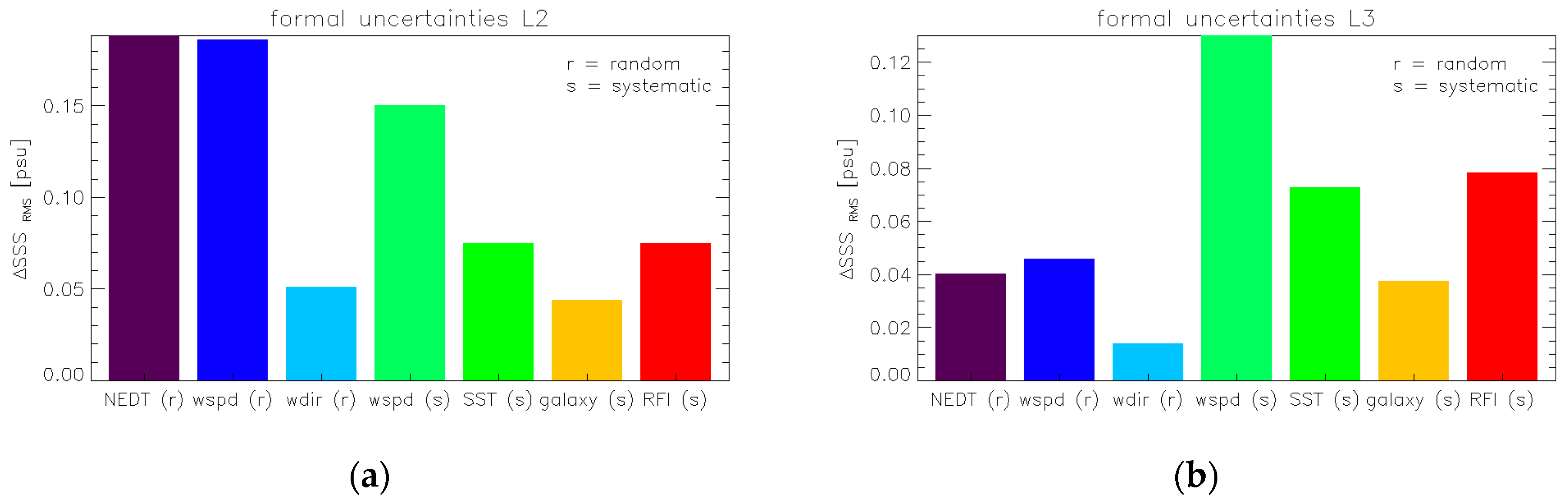
Figure 12 shows the contributions of the various components of the error model (Section 8.2) to the total formal uncertainty estimate for (a) the Aquarius L2 product (1.44 s) and (b) the monthly 1° L3 salinity product, respectively. The dominant contributions at the 1.44 s are the NEDT and the random and systematic uncertainties in the wind speed that is used in the surface roughness correction algorithm. At the monthly 1° Level 3 product all the random uncertainties including the NEDT are reduced to low levels. The dominant uncertainty contribution at the monthly L3 product is the systematic uncertainty in the HHH wind speed.

9. Validation and Improvements from Previous Releases

The ultimate assessment of the performance of the Aquarius Version 5 salinity algorithm is done by comparing the Aquarius Version 5 salinity retrievals with other salinity measurements and sources such as ARGO or HYCOM.

A comprehensive validation analysis for the Aquarius Version 5 products have been performed in [32,33]. The root mean square error (RMSE) of the Aquarius Version 5 salinity have been estimated from a triple point analysis using individual match-ups between Aquarius, ARGO floats and HYCOM. The estimated RMSE for Aquarius is 0.17 psu for the Level 2 product (1.44 s) and 0.128 psu for monthly 100 km averages. For computing this value, observations in very cold water (SST < 5 °C) where the sensitivity is low were excluded. These values are significantly better than the Aquarius prime mission requirement, which allocated and RMSE of 0.2 psu for monthly 100 km averages.

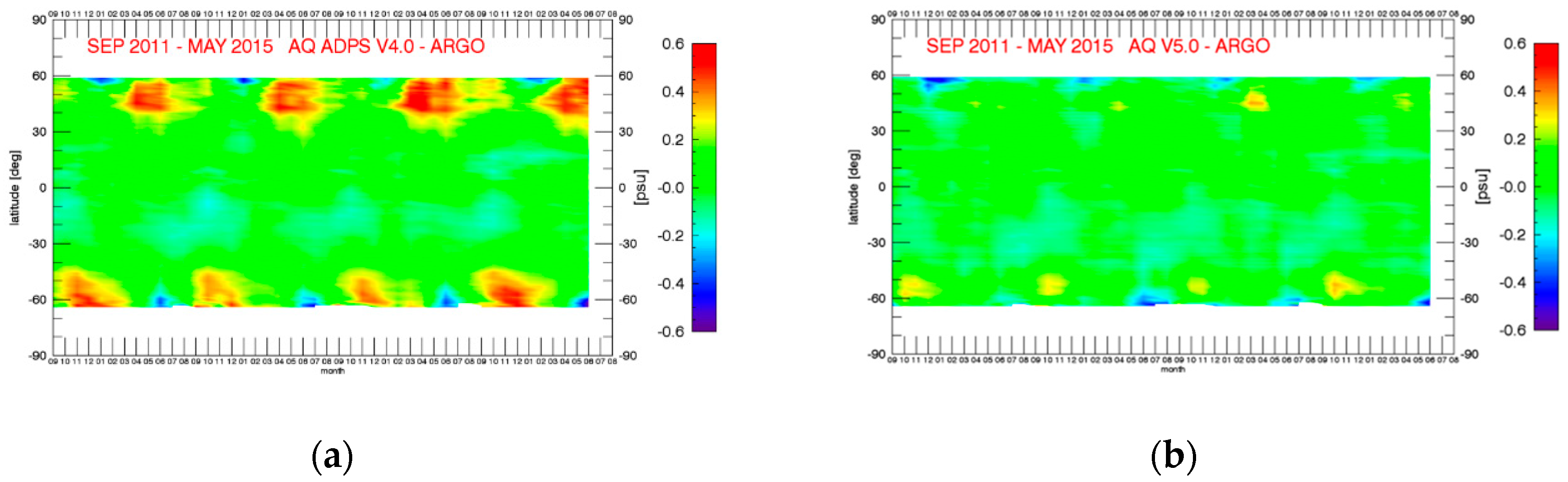
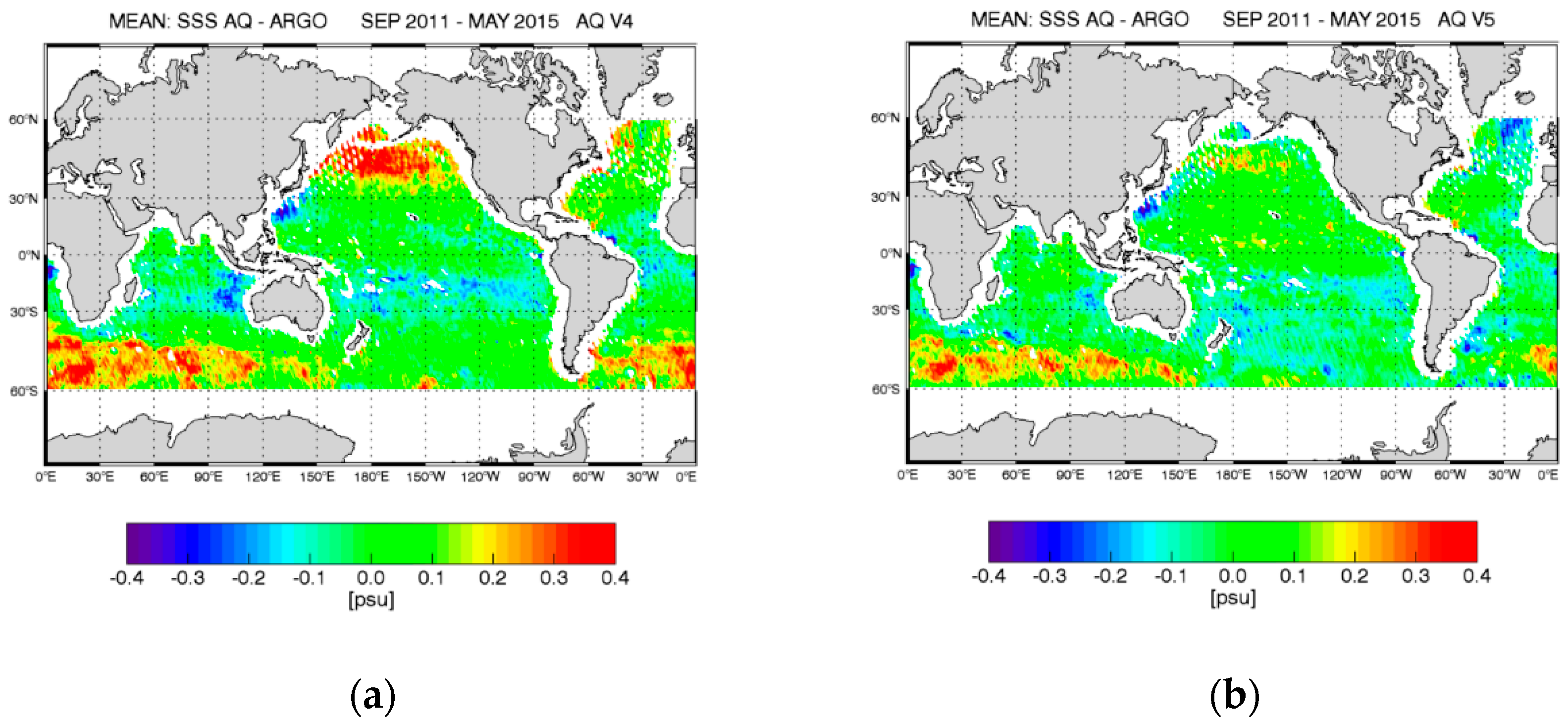
It is also worthwhile to look how the improvements in the Version 5 algorithm compared with previous releases and match the steps in the algorithm updates these performance improvements. A good way to do this is to analyze time—latitude Hovmoeller diagrams (Figure 13) and maps of global differences (Figure 14) between Aquarius and Scripps ARGO (Section 2.3) salinity fields. For computing these figures the Aquarius observations in rain were filtered out in order to exclude mismatches between Aquarius and the ARGO due to stratification on the upper ocean layer that can occur in precipitating scenes (see Section 2.2.6). Both figures show clear improvement in Version 5 for most of the temporal and zonal biases that were observed in the Version 4 and earlier releases. The reduction of the salty biases at mid-high latitudes, which were particularly strong in the NW and N Pacific during April—June and in the S Atlantic and S Indian Ocean during October - December are mainly due to the change in the atmospheric oxygen absorption model (Section 4.2) and partly also to the changes in the SST dependence of the wind induced emissivity (Section 3). The small improvements in the fresh biases at high S latitudes during the summer months can be traced back to the changes in the reflected galaxy correction (Section 5).

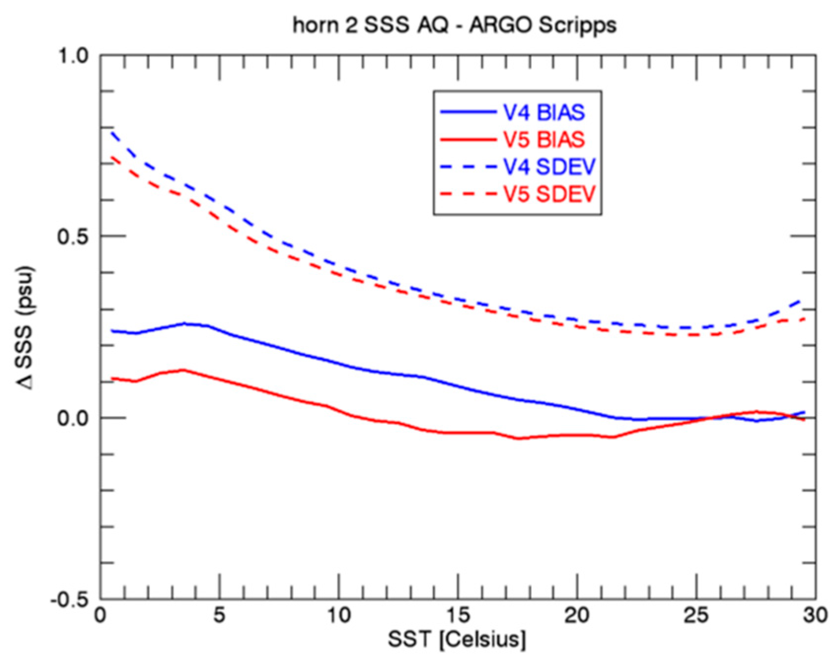
Another important achievement in the performance of the Version 5 salinity retrievals is evident from Figure 15, which shows bias and standard deviation of- the difference between the Aquarius Level 2 salinity and Scripps ARGO as function of SST for both Version 4 and Version 5. In Version 5 the difference between Aquarius Version 5 and ARGO is within ±0.1 psu, even in very cold water. That applies to all 3 Aquarius horns. That means that with the algorithm updates in Version 5 the SST dependent biases that have been observed in earlier releases [4] have been essentially eliminated. We note that the difference between Aquarius Version 5 and ARGO is also within ±0.1 psu if the stratification is done as a function of wind speed.

Despite the significant improvements in Aquarius Version 5 from prior releases, Figure 14b still indicates noticeable residual biases in some areas, for example salty biases in the S Atlantic and S Indian Ocean. The cause of these residual biases is currently not fully understood. So, there is still room for some improvements of the Aquarius salinity algorithm in possible future releases. We also want to be clear that it might well be possible to use a different geophysical model function than the one that we have used for the Aquarius Version 5 release and presented here, which might result in the same or even better performance. Such a change in the geophysical model could, for example include a different model for the dielectric constant of sea water.

10. Adaption to Version 3 SMAP Salinity Retrievals

The last section in this paper deals with the adaption of the Aquarius Version 5 salinity retrieval algorithm to SMAP. Specifically, we are considering the NASA RSS (Remote Sensing Systems) SMAP Version 3 salinity release, which is scheduled for late summer 2018. For most of the part, adapting the Aquarius salinity retrieval algorithm (Figure 1) is rather straightforward and amounts to deriving or interpolating the corrections that were derived for Aquarius to the SMAP orbit and pointing. There are two important exceptions, which we discuss in the following.

10.1. SMAP Emissive Reflector

The emissivity of the Aquarius antenna was negligibly small for all practical purposes. However, the SMAP mesh reflector has an emissivity of about 1%, which is large enough so that a correction needs to be applied in the salinity retrieval [7]. If $T_A$ is the antenna temperature before the radiation hits the reflector whose physical temperature is denoted by $T_{refl}$ and whose emissivity is ${\epsilon }_{refl}$, then after antenna temperature $T_A^{\prime }$ after the reflection, which enters the receiver, is given by:

$$T_A^{\prime }=\left(1-{\epsilon }_{refl}\right)\cdot T_A+{\epsilon }_{refl}\cdot T_{refl}=T_A+{\epsilon }_{refl}\cdot \left(T_{refl}-T_A\right).$$

(15)

In order to perform the correction, i.e., determine the value of $T_A$ from the measured $T_A^{\prime }$ according to Equation (15), it is necessary to know the values of both the reflector emissivity ${\epsilon }_{refl}$ and its physical temperature $T_{refl}$.

The value of the reflector emissivity ${\epsilon }_{refl}$ can be determined by performing a linear regression of the SMAP $\Delta T_A=T_{A,meas}-T_{A,\exp }$ against $T_{refl}-T_{A,meas}$ before performing any correction for the emissive reflector. The slope of this regression is ${\epsilon }_{refl}$. We have determined values of ${\epsilon }_{refl}=0.01012$ for both V-pol and H-pol. It is worth to point out that these values for the reflector emissivity are about 4 times larger than the values that were determined pre-launch.

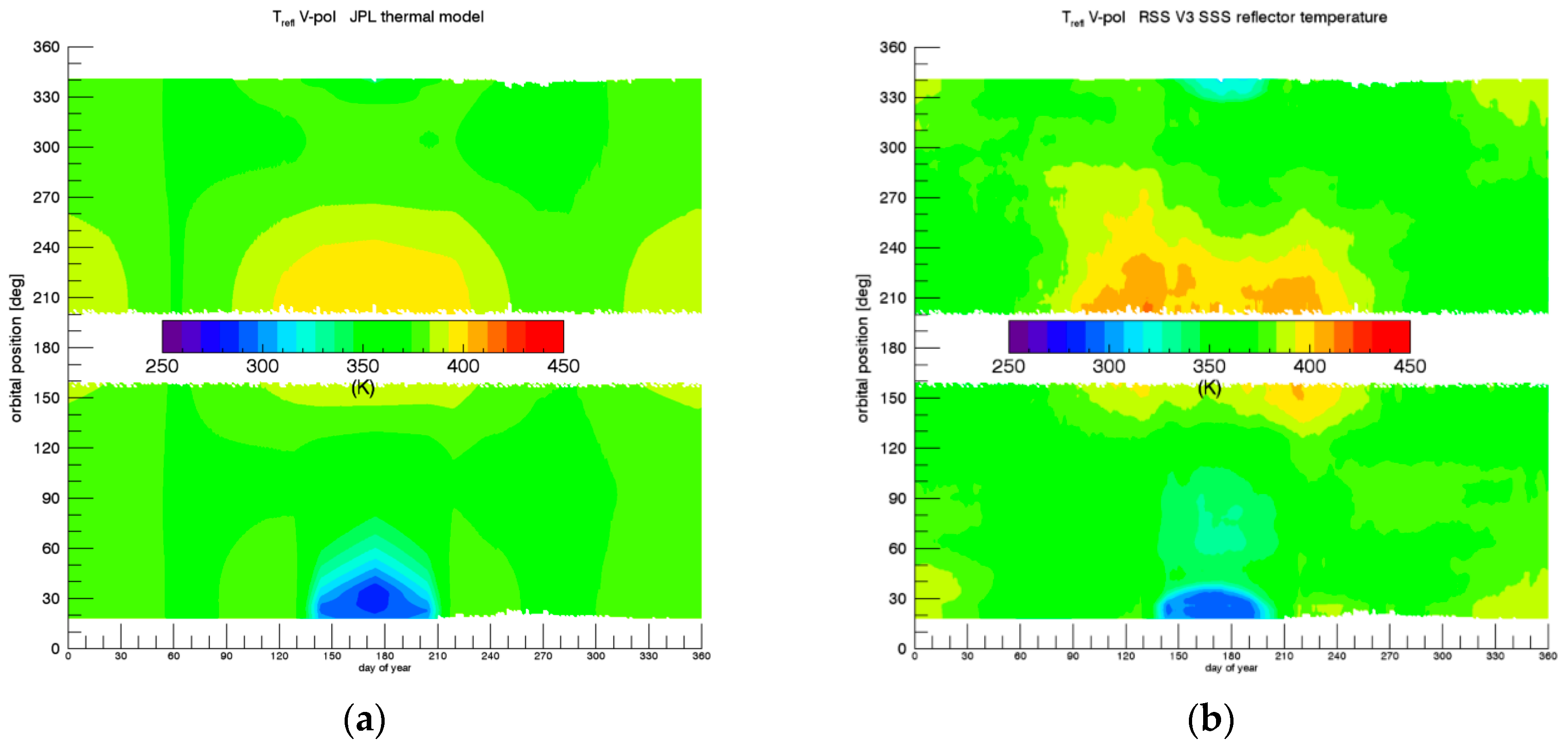
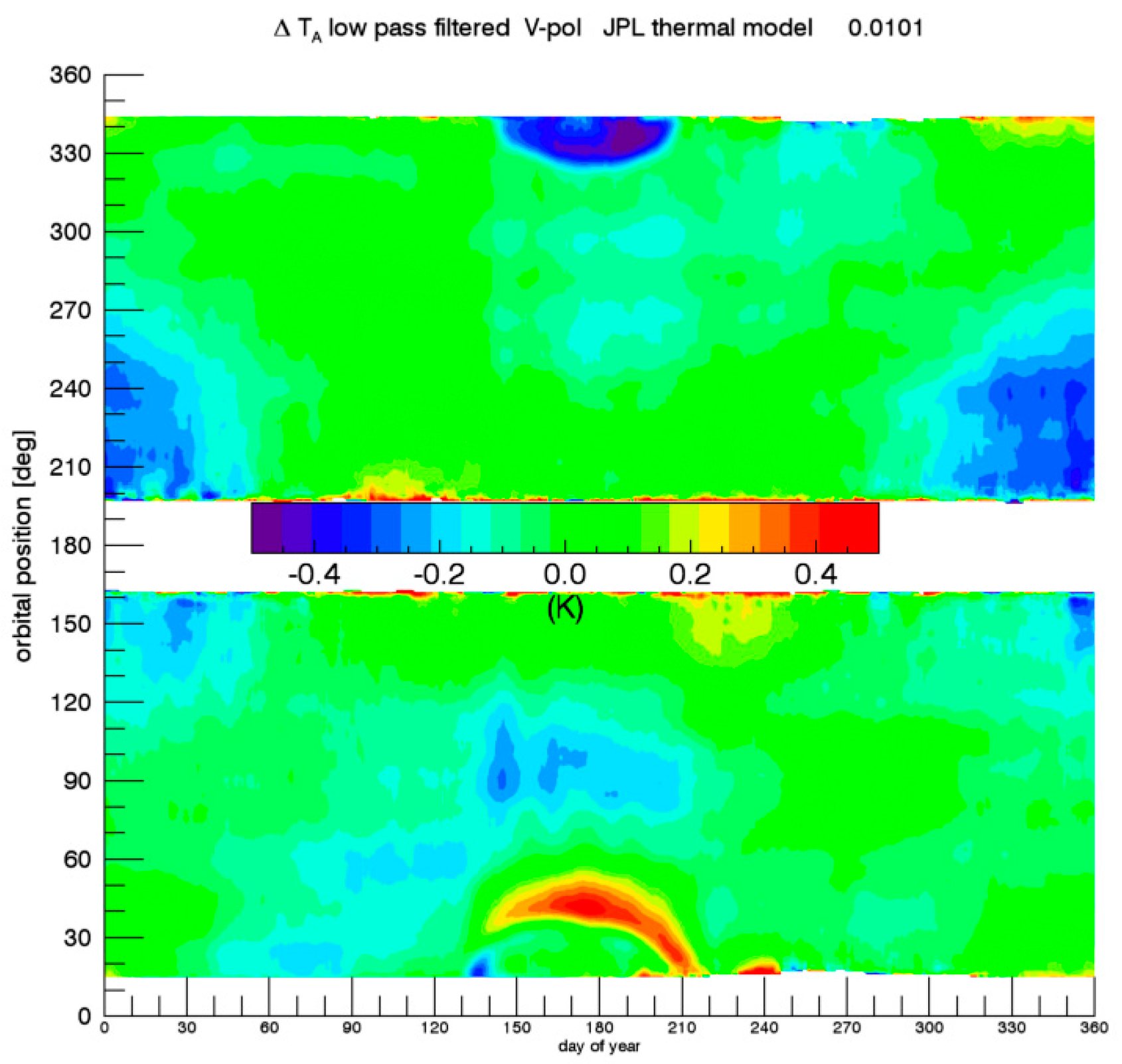
Unfortunately, there are no direct measurements of the physical temperature $T_{refl}$ of the SMAP mesh antenna. Only the results of thermal model for the SMAP reflector, which was developed and run by the Jet Propulsion Laboratory (JPL) thermal modeling team is available (Figure 16a). The values of this JPL thermal model are used and included in the SMAP L1B files [34]. Our analysis has revealed that the JPL thermal model is not accurate enough to retrieve ocean salinity from SMAP without adjustments. This can be seen from the Hovmoeller diagram in Figure 17, which shows the bias of $T_{A,meas}-T_{A,\exp }$ as function to time (day of year) and orbital position (z-angle) if the JPL thermal model is used in the emissive reflector correction. In the computation of $T_{A,\exp }$ we have used Scripps ARGO as reference salinity (Section 2.3). The zonal and temporal biases get large when the spacecraft goes in and out of solar eclipse during the summer months and it is also large during the winter months. In those instances, rapid cooling or heating of the SMAP reflector occurs. Apparently, the thermal models can overestimate or underestimate the rate of these thermal changes. The observed zonal and temporal biases in Figure 17 are largely independent of the SMAP look direction. They differ significantly between ascending (lower half of the diagram) and descending (upper half of the diagram) swaths, because the thermal heating and cooling of the SMAP antenna is not symmetric between the two swaths. That makes us believe that they are indeed caused by inaccuracies in the JPL thermal model rather than by other sources. For example errors in the correction for galaxy or sun intrusion would strongly depend on look direction. On the other hand, errors in dielectric model or surface roughness correction are expected to be largely the same in the ascending and descending swaths. It was decided for SMAP salinity retrievals to make an empirical adjustment to the JPL thermal model, whose purpose is to minimize the zonal and temporal biases in $\Delta T_A=T_{A,meas}-T_{A,\exp }$ when the correction for the emissive reflector is performed with this empirical adjusted model. This can be done by taking the values for the $\Delta T_A$ biases from Figure 17 and computing the corresponding biases of $\Delta T_{refl}$ using (15). The result for the empirical adjusted thermal model in the SMAP Version 3 salinity release is shown in Figure 16b. We use the same thermal model adjustments for V-pol and H-pol.

A final note in our approach of the empirical determination of both ${\epsilon }_{refl}$ and $T_{refl}$ for SMAP concerns the fact that we have tried to avoid folding a potential error in one quantity into the other. When determining the value of ${\epsilon }_{refl}$ from the linear regression, we have used only cases where we can regard the JPL thermal model as accurate, i.e., where the biases in Figure 17 are small (less than 0.1 K).

10.2. SMAP Surface Roughness Correction

The second major difference between Aquarius and SMAP that needs to be taken into account when transferring the Aquarius Version 5 salinity retrieval algorithm to SMAP is the surface roughness correction. The crucial ancillary input to the surface roughness correction is the surface wind speed. The Aquarius salinity retrievals use the Aquarius HHH wind speed, which is obtained from the Aquarius HH-pol L-band scatterometer and H-pol radiometer observations [3,12]. For the SMAP salinity retrievals scatterometer observations are not available, as the SMAP radar failed in July 2015. It is necessary to use an external ancillary wind speed in the SMAP salinity retrieval algorithm, as the two SMAP radiometer channels (V-pol and H-pol) do not carry sufficient information to perform the surface roughness correction without ancillary wind speed input. For the SMAP Version 3 it was decided to use the CCMP (Cross Calibrated Multi-Platform) Version 2.0 wind fields [35,36,37] as ancillary input for both wind speed and wind direction. CCMP is a gridded (0.25°) Level 4 wind vector product that combines various satellite wind measurements from the RSS Version 7 ocean suite with a background field from a numerical weather prediction model using a variational assimilation method (VAM). A near-real time (NRT) version of CCMP V2.0 is produced at RSS, whose latency is short enough to be used as ancillary input in the Version 3 SMAP salinity retrievals. This NRT V2.0 CCMP wind product currently ingests RSS V7.0 WindSat, GMI, SSMIS and AMSR2 wind speed observations and uses NCEP GDAS 0.25° wind speed and direction as background field.

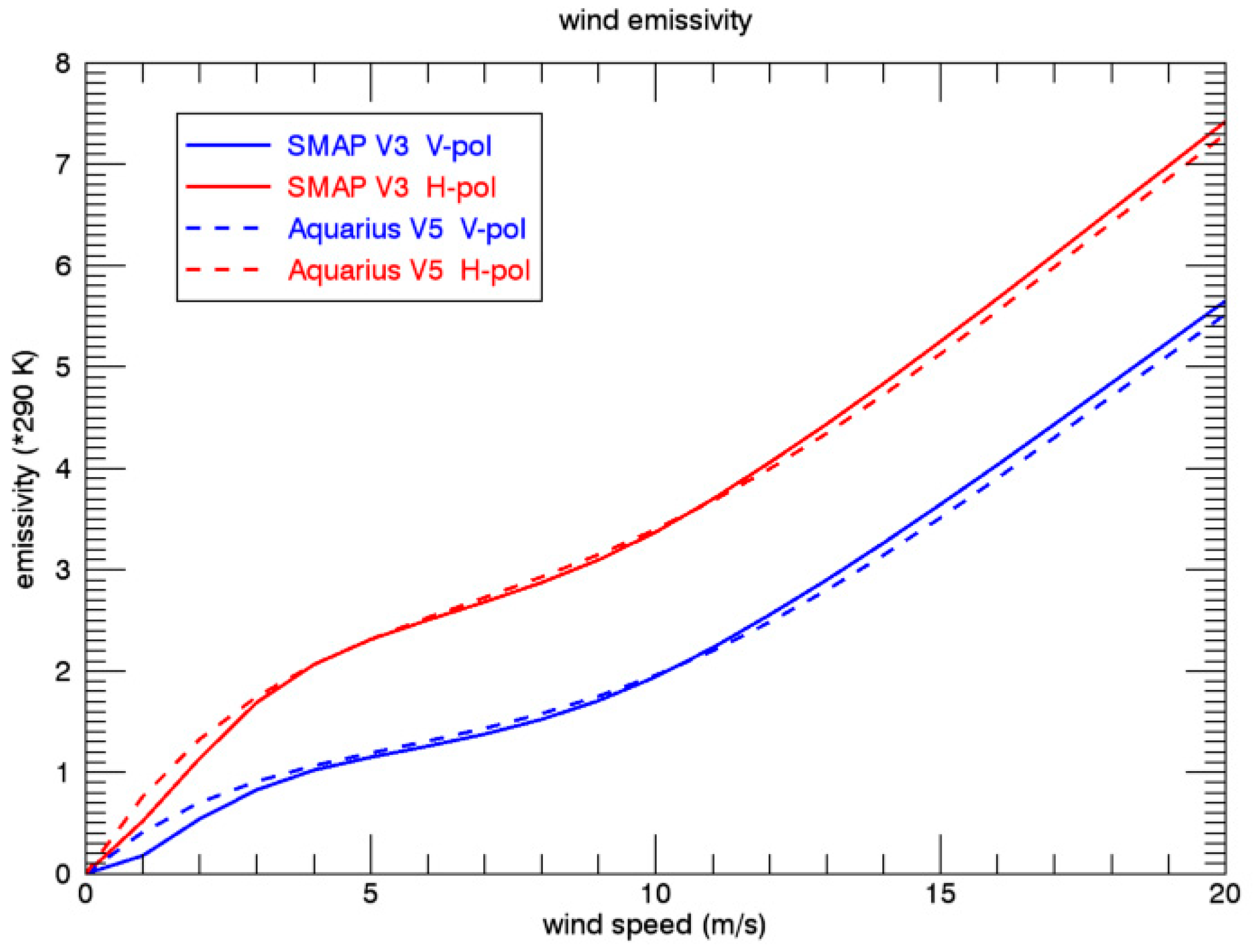
The crucial point for developing the geophysical model of the wind induced emissivity for SMAP Version 3 is that the CCMP ancillary field is slightly different from the Aquarius HHH wind speed that has been used in the Aquarius Version 5 algorithm. That means that there are small biases in the order of a few tenth of m/s between these two ancillary wind fields and these biases depend on wind speed and also on SST. Because of the high level of accuracy that is required for retrieving salinity, these biases need to be taken into account when deriving the wind induced emissivity model function for SMAP Version 3 using the method outlined in [12]. As a consequence of the slightly different ancillary wind speed inputs to the Aquarius Version 5 and SMAP Version 3 salinity retrieval algorithms, the geophysical model functions for the wind emissivities also slightly differ. This is most important for the wind speed dependence 0th harmonic coefficient of the wind induced emissivity, i.e., the isotropic part. This is shown in Figure 18 for both SMAP polarizations. Small differences are observable at very low and at very high wind speeds. This coincides with the instances where small differences between Aquarius HHH and CCMP wind speeds exist. In addition, we have also found slight differences in the SST dependence $\rho \left(T_S\right)$ (c.f. Section 3) of the wind induced emissivity, which is shown in Figure 2 for the h-pol. The term ${\rho }^{\prime }\left(T_S\right)$ in Equation (1), which is empirically determined and which is the deviation from the theoretical value predicted by the geometric optics model, is half as large in SMAP Version 3 than it was in Aquarius Version 5. Consequently, the value of $\rho \left(T_S\right)$ in SMAP Version 3 lies between the theoretical value of the geometrics optics model, which is given by $E_0\left(T_S\right)/E_0\left(T_{ref}\right)$, and the value of Aquarius Version 5.

11. Summary and Conclusions

To summarize our main results:

Our paper gives an overview of the steps in the salinity retrieval algorithm for Aquarius Version 5. We have highlighted and elaborated on the issues that have not been previously published or that are new and that help improving the performance of Version 5 from previous releases. The most important components are the corrections for the absorption by atmospheric oxygen, the SST dependence of the surface roughness correction and the reflected galaxy correction. The Aquarius Version 5 reflected galaxy correction requires an empirical zonal symmetrization to remove spurious biases between the ascending and descending Aquarius orbit segments. The ocean target calibration effectively constraints the global average of the Aquarius salinity to the value from ARGO. This is necessary to determine the main calibration parameters of the internal radiometer calibration references (noise-diode injection temperatures) and to accurately correct temporal drifts in the calibration system. A comparison with ground truth observations from ARGO floats shows that most of the temporal and zonal biases that have been identified in previous Aquarius releases have been removed or reduced to a low level in the Version 5 release. The accuracy of Aquarius Version 5 is significantly better than the prime mission requirement of 0.2 psu. The Aquarius Version 5 salinity retrievals are accompanied by estimates for random and systematic uncertainties. The basis for these uncertainty estimates in the salinity retrievals are realistic estimates of the uncertainties in the input parameters to the algorithm.

The Aquarius Version 5 salinity retrieval algorithm can be adapted to SMAP, which is straightforward for most parts. Important differences between Aquarius and SMAP that need to be taken into account are the correction for the emissive SMAP antenna and the wind induced emissivity.

Our analysis has also shown that there is still room and necessity of further improvements in the salinity retrieval algorithms for both instruments. This will be part of future releases. Direct comparisons between the retrieved Aquarius Version 5 and SMAP Version 3 salinities will be an important tool in analyzing remaining biases and in deriving future algorithm improvements.

References

- Le Vine, D.; Lagerloef, G.; Colomb, F.; Yueh, S.; Pellerano, F. Aquarius: An instrument to monitor sea surface salinity from space. IEEE Trans. Geosci. Remote Sens. 2007, 45, 2040–2050. [Google Scholar] [CrossRef]
- Aquarius Official Release Level 2 Sea Surface Salinity & Wind Speed Data V5.0. Available online: https://podaac.jpl.nasa.gov/dataset/AQUARIUS_L2_SSS_V5 (accessed on 10 July 2018).
- Meissner, T.; Wentz, F.; Le Vine, D. Aquarius Salinity Retrieval Algorithm Theoretical Basis Document (ATBD), End of Mission Version; RSS Technical Report 120117. 1 December 2017. Available online: http://podaac-ftp.jpl.nasa.gov/allData/aquarius/docs/v5/AQ-014-PS-0017_Aquarius_ATBD-EndOfMission.pdf (accessed on 10 July 2018).
- Le Vine, D.; Dinnat, E.; Meissner, T.; Yueh, S.; Wentz, F.; Torrusio, S.; Lagerloef, G. Status of Aquarius/SAC-D and Aquarius salinity retrievals. IEEE J. Sel. Top. Appl. Earth Obs. Remote Sens. 2015, 8, 5401–5415. [Google Scholar] [CrossRef]
- Entekhabi, D.; Joku, E.G.; O’Neill, P.E.; Kellogg, K.H.; Crow, W.T.; Edelstein, W.N.; Entin, J.K.; Goodman, S.D.; Jackson, T.J.; Johnson, J.; et al. The Soil Moisture Active Passive (SMAP) mission. Proc. IEEE 2010, 98, 704–716. [Google Scholar] [CrossRef]
- Peng, J.; Misra, S.; Piepmeier, J.R.; Dinnat, E.P.; Hudson, D.; Le Vine, D.M.; De Amici, G.; Mohammed, P.N.; Bindlish, R.; Yueh, S.H.; et al. Soil Moisture Active/Passive L-Band microwave radiometer postlaunch calibration. IEEE Trans. Geosci. Remote Sens. 2017, 55, 5339–5354. [Google Scholar] [CrossRef]
- RSS SMAP Level 2C Sea Surface Salinity V2.0 Validated Dataset. Available online: https://podaac.jpl.nasa.gov/dataset/SMAP_RSS_L2_SSS_V2 (accessed on 10 July 2018).
- Misra, S.; Ruf, C. Detection of radio-frequency interference for the Aquarius radiometer. IEEE Trans. Geosci. Remote Sens. 2008, 46, 3123–3128. [Google Scholar] [CrossRef]
- Le Vine, D.; de Matthaeis, P.; Ruf, C.; Chen, D. Aquarius RFI Detection and Mitigation Algorithm: Assessment and Examples. IEEE Geosci. Remote Sens. 2014, 52, 4574–4584. [Google Scholar] [CrossRef]
- Meissner, T.; Wentz, F. The complex dielectric constant of pure and sea water from microwave satellite observations. IEEE Trans. Geosci. Remote Sens. 2004, 42, 1836–1849. [Google Scholar] [CrossRef] [Green Version]
- Meissner, T.; Wentz, F. The emissivity of the ocean surface between 6 and 90 GHz over a large range of wind speeds and Earth incidence angles. IEEE Trans. Geosci. Remote Sens. 2012, 50, 3004–3026. [Google Scholar] [CrossRef]
- Meissner, T.; Wentz, F.; Ricciardulli, L. The emission and scattering of L-band microwave radiation from rough ocean surfaces and wind speed measurements from Aquarius. J. Geophys. Res. Oceans 2014, 119. [Google Scholar] [CrossRef]
- Meissner, T.; Wentz, F.; Scott, J.; Vasquez-Cuervo, J. Sensitivity of ocean surface salinity measurements from spaceborne L-Band radiometers to ancillary sea surface temperature. IEEE Trans. Geosci. Remote Sens. 2016, 54, 7105–7111. [Google Scholar] [CrossRef]
- Boutin, J.; Chao, Y.; Asher, W.E.; Delcroix, T.; Drucker, R.; Drushka, K.; Kolodziejczyk, N.; Lee, T.; Reul, N.; Reverdin, G.; et al. Satellite and in situ salinity: Understanding near-surface stratification and subfootprint variability. Bull. Am. Meteorol. Soc. 2016, 97, 1391–1407. [Google Scholar] [CrossRef]
- Santos-Garcia, A.; Jacob, M.; Jones, W.L.; Asher, W.; Hejazin, Y.; Ebrahimi, H.; Rabolli, M. Investigation of rain effects on Aquarius sea surface salinity measurements. J. Geophys. Res. Oceans 2014, 119, 7605–7624. [Google Scholar] [CrossRef]
- Joyce, R.; Janowiak, J.; Arkin, P.; Xie, P. CMORPH: A method that produces global precipitation estimates from passive microwave and infrared data at high spatial and temporal resolution. J. Hydrometeorol. 2004, 5, 487–503. [Google Scholar] [CrossRef]
- Wentz, F.; Meissner, T. Algorithm Theoretical Basis Document (ATBD), Version 2, AMSR Ocean Algorithm, RSS Tech. Report 121599A-1. Available online: http://images.remss.com/papers/rsstech/2000_121599A-1_Wentz_AMSR_Ocean_Algorithm_ATBD_Version2.pdf (accessed on 10 July 2018).
- Wentz, F.; Meissner, T. Atmospheric absorption model for dry air and water vapor at microwave frequencies below 100 GHz derived from spaceborne radiometer observations. Radio Sci. 2016, 51, 381–391. [Google Scholar] [CrossRef]
- Liebe, H.; Rosenkranz, P.; Hufford, G. Atmospheric 60-GHz oxygen spectrum: New laboratory measurements and line parameters. J. Quant. Spectrosc. Radiat. Transf. 1992, 48, 629–643. [Google Scholar] [CrossRef]
- Le Vine, D.; Abraham, S. Galactic noise and passive microwave remote sensing from space at L-band. IEEE Trans. Geosci. Remote Sens. 2004, 42, 119–129. [Google Scholar] [CrossRef] [Green Version]
- Dinnat, E.; Le Vine, D.; Abraham, S.; Floury, N. Map of Sky Background Brightness Temperature at L-Band. Available online: https://podaac-tools.jpl.nasa.gov/drive/files/allData/aquarius/L3/mapped/galaxy/2018 (accessed on 7 July 2018).
- Wentz, F. The forward scattering of microwave solar radiation from a water surface. Radio Sci. 1978, 13, 131–138. [Google Scholar] [CrossRef] [Green Version]
- Cox, C.; Munk, W. Measurement of the roughness of the sea surface from photographs of the sun’s glitter. J. Opt. Soc. Am. 1954, 44, 838–850. [Google Scholar] [CrossRef]
- Piepmeier, J. Calibration of passive microwave polarimeters that use hybrid coupler-based correlators. IEEE Trans. Geosci. Remote Sens. 2004, 43, 391–400. [Google Scholar] [CrossRef]
- Misra, S.; Brown, S. Enabling the extraction of climate-scale temporal salinity variations from Aquarius: An instrument based long-term radiometer drift correction. IEEE Trans. Geosci. Remote Sens. 2017, 55, 2913–2923. [Google Scholar] [CrossRef]
- Dinnat, E.; Le Vine, D. Cold sky calibration (CSC) biases and time Series with hardware-only wiggle correction. Presented at the Aquarius Cal/Val Meeting, Santa Rosa, CA, USA, 9–11 January 2017; Available online: https://aquarius.umaine.edu/cgi/meetings.htm (accessed on 7 July 2018).
- Meissner, T. Assessment of Uncertainties in Aquarius Salinity Retrievals, RSS Technical Report 061015. 10 June 2015. Available online: http://podaac-ftp.jpl.nasa.gov/allData/aquarius/docs/v4/AQ-014-PS-0017_AquariusATBD_uncertainties_Addendum5_DatasetVersion4.0.pdf (accessed on 7 July 2018).
- Meissner, T.; Wentz, F.; Le Vine, D.; Lee, T. Estimate of uncertainties in the Aquarius salinity retrievals. In Proceedings of the 2015 IEEE International Geoscience and Remote Sensing Symposium (IGARSS), Milan, Italy, 26–31 July 2015; pp. 5324–5327. Available online: http://images.remss.com/papers/rssconf/Meissner_igarss_2015_Milan_AquariusErrors.pdf (accessed on 7 July 2018). [CrossRef]
- Wentz, F.; Ricciardulli, L.; Gentemann, C.; Meissner, T.; Hilburn, K.; Scott, J. Remote Sensing Systems Coriolis WindSat Environmental Suite on 0.25 deg Grid, Version 7.0.1, Remote Sensing Systems. Santa Rosa, CA, 2013. Available online: www.remss.com/missions/windsat (accessed on 7 July 2018).
- Yu, T.-W.; Gerald, V.M. Evaluation of NCEP operational model forecasts of surface wind and pressure fields over the oceans. In Proceedings of the 20th Conference on Weather Analysis and Forecasting/16th Conference on Numerical Weather Prediction. 2004. Available online: http://polar.ncep.noaa.gov/mmab/papers/tn233/mmab233.pdf (accessed on 7 July 2018).
- Ricciardulli, L.; Meissner, T.; Wentz, F. Towards a climate data record of satellite ocean vector winds. In Proceedings of the 2012 IEEE International Geoscience and Remote Sensing Symposium (IGARSS), Munich, Germany, 22–27 July 2012; pp. 2067–2069. Available online: http://images.remss.com/papers/rssconf/ricciardulli_igarss_2012_munich.pdf (accessed on 7 July 2018). [CrossRef]
- Aquarius Salinity Validation Analysis (Data Version 5.0). Available online: https://podaac.jpl.nasa.gov/dataset/AQUARIUS_L2_SSS_V5?ids=SpatialCoverage:TemporalResolution&values=Global:Weekly (accessed on 7 July 2018).
- Kao, H.-Y.; Lagerloef, G.; Lee, T.; Melnichenko, O.; Meissner, T.; Hacker, P. Assessment of Aquarius Sea Surface Salinity Data using Aquarius Validation Data System (AVDS) and other statistical methods. Remote Sens. 2018. submitted. [Google Scholar]
- Piepmeier, J.; Mohammed, P.; Peng, J.; Kim, E.; De Amici, G.; Ruf, C. SMAP L1B Radiometer Half-Orbit Time-Ordered Brightness Temperatures; Version 3; CRID 13080; NSIDC: Boulder, CO, USA, 2016. [Google Scholar] [CrossRef]
- Atlas, R.; Hoffman, R.; Ardizzone, J.; Leidner, S.M.; Jusem, J.; Smith, D.; Gombos, D. A cross-calibrated, multiplatform ocean surface wind velocity product for meteorological and oceanographic applications. Bull. Am. Meteorol. Soc. 2011, 92, 157–174. [Google Scholar] [CrossRef]
- Wentz, F.; Scott, J.; Hoffman, R.; Leidner, M.; Atlas, R.; Ardizzone, J. Remote Sensing Systems Cross-Calibrated Multi-Platform (CCMP) 6-Hourly Ocean Vector Wind Analysis Product on 0.25 deg Grid; Version 2.0; Remote Sensing Systems: Santa Rosa, CA, USA, 2015; Available online: http://www.remss.com/measurements/ccmp (accessed on 7 July 2018).
- Ricciardulli, L.; National Center for Atmospheric Research Staff (Eds.) The Climate Data Guide: CCMP: Cross-Calibrated Multi-Platform Wind Vector Analysis. 2017. Available online: https://climatedataguide.ucar.edu/climate-data/ccmp-cross-calibrated-multi-platform-wind-vector-analysis (accessed on 7 July 2018).
Figure 1.
Schematic flow diagram of the Aquarius Version 5 salinity retrieval algorithm.
Figure 2.
SST dependence of the wind induced emissivity for Aquarius horn 2 H-pol. The blue line in the SST dependence from [12], which is predicted by the geometric optics model for the wind induced surface emission and which was used in earlier Aquarius releases. The red line is the SST dependence used in the Aquarius Version 5 release. The green line is the SST dependence used in the SMAP Version 3 release (Section 10).
Figure 3.
Effect of atmospheric absorption: Top of the atmosphere TB minus surface TB for Aquarius H-pol horn 2 (in Kelvin). The figure shows the difference between the O2 absorption model by Liebe et al. [19], which is used in the Version 5 algorithm and the Wentz Meissner O2 absorption model [18], which had been used in prior versions.
Figure 4.
Difference of ascending minus descending the TA measured—expected (in Kelvin) for Aquarius horn 2 using the reflected galaxy from the GO model. The figure shows the value of the average as function of time (SEP 2011–JUN 2015) and latitude.
Figure 5.
Difference of ascending minus descending the TA measured—expected (in Kelvin) for Aquarius horn 2 using the reflected galaxy from the SMAP fore—aft analysis. The figure shows the value of the average as function of time (SEP 2011–JUN 2015) and latitude.
Figure 6.
(a) Reflected galactic radiation computed from the GO model for an average wind speed of 7.5 m/s. (b) Value of the empirical symmetrization Δ derived in this section. The figures show the values of the averages (in Kelvin) as function of time (day of year) and orbital position (z-angle) for Aquarius horn 2.
Figure 7.
Same as Figure 5 but after applying the empirical symmetrization correction.
Figure 8.
Comparison between Aquarius horn 2 and HYCOM salinity as function of the logarithmic gain weighted land fraction gland. Blue: Without correction for land intrusion. Red: With correction for land intrusion. (a) Bias. (b) Standard deviation.
Figure 9.
Map of the salinity difference between ascending (asc) and descending (dsc) Aquarius swaths for SEP 2011–AUG 2014.
Figure 10.
(a) RFI peak hold map: The map shows the largest monthly average value of the difference between RFI-filtered (TF) and unfiltered (TA) antenna temperatures over the time period SEP 2011–AUG 2014 of the ascending Aquarius swath. In producing the figure we have averaged over all 3 horns. (b) RFI mask for the ascending Aquarius swath: The map is obtained from the peak-hold map in (a) by taking all cells for which |TF − TA| > 0.2 K and then extending this area by ±4°. This mask indicates the geographical area where undetected RFI might be present.
Figure 11.
Estimated uncertainty in the retrieved Aquarius salinity due to undetected RFI for the ascending swath (a) and the descending swath (b). In producing the figures we have averaged over all 3 horns.
Figure 12.
Contribution of the various uncertainties to the total estimated uncertainty for open ocean scenes of: (a) the Aquarius Level 2 salinity that is observed at the 1.44 s cycle; (b) the 1° Aquarius Level 3 salinity maps.
Figure 13.
Hovmoeller plot of the difference between Aquarius and Scripps ARGO salinity. Panel (a) is for the Version 4 release. Panel (b) is for the Version 5 release. The x-axis in both plots is the time (month) over the time period September 2011–May 2015. The y-axis is the latitude. For the comparison Aquarius observations containing rain have been discarded (see Section 2.2.6).
Figure 14.
Average difference between Aquarius and Scripps ARGO over the time period September 2011–May 2015. Panel (a) is for the Version 4 release. Panel (b) is for the Version 5 release. For the comparison observations containing rain have been discarded (see Section 2.2.6).
Figure 15.
Difference between L2 Aquarius horn 2 and Scripps ARGO salinity as function of SST. The blue curves are for the Version 4 release. The red curves are for the Version 5 release. Full lines show the biases and dashed lines show the standard deviations. For the comparison observations containing rain have been discarded (see Section 2.2.6).
Figure 16.
Physical temperature of the reflector. (a) JPL thermal model that is used in the SMAP L1B files [34]. (b) Empirical adjustment in the RSS SMAP Version 3 salinity release.
Figure 17.
Hovmoeller diagram of SMAP over the open ocean using the JPL thermal model for the SMAP mesh antenna. The x-axis is time (day of year) and the y-axis is orbital position (z-angle). For the computation of we have used Scripps ARGO as reference salinity (Section 2.3). The computation of this diagram is based on 2 years of SMAP data (September 2015–August 2017). A simple spatial and temporal low-pass filter was applied by performing a running average in both dimensions.
Figure 18.
Isotropic (wind-direction independent) part of the wind induced emissivity that is used in the Aquarius Version 5 after interpolating to the SMAP Earth Incidence Angle (dashed lines) and the SMAP Version 3 (full lines) releases. Blue: V-pol. Red: H-pol. The figure shows the 0th harmonic of the wind induced excess emissivity [3,12] multiplied by 290 K.
© 2018 by the authors. Licensee MDPI, Basel, Switzerland. This article is an open access article distributed under the terms and conditions of the Creative Commons Attribution (CC BY) license (http://creativecommons.org/licenses/by/4.0/).
Share and Cite
MDPI and ACS Style
Meissner, T.; Wentz, F.J.; Le Vine, D.M. The Salinity Retrieval Algorithms for the NASA Aquarius Version 5 and SMAP Version 3 Releases. Remote Sens. 2018, 10, 1121. https://doi.org/10.3390/rs10071121
AMA Style
Meissner T, Wentz FJ, Le Vine DM. The Salinity Retrieval Algorithms for the NASA Aquarius Version 5 and SMAP Version 3 Releases. Remote Sensing. 2018; 10(7):1121. https://doi.org/10.3390/rs10071121
Chicago/Turabian StyleMeissner, Thomas, Frank J. Wentz, and David M. Le Vine. 2018. "The Salinity Retrieval Algorithms for the NASA Aquarius Version 5 and SMAP Version 3 Releases" Remote Sensing 10, no. 7: 1121. https://doi.org/10.3390/rs10071121
Note that from the first issue of 2016, this journal uses article numbers instead of page numbers. See further details here.