Fusion of Moderate Resolution Earth Observations for Operational Crop Type Mapping
by
Nathan Torbick
1,*, 
Xiaodong Huang
1,
Beth Ziniti
1,
David Johnson
2,
Jeff Masek
3 and
Michele Reba
4 1
Applied Geosolutions, 15 Newmarket Rd, Durham, NH 03824, USA
2
United States Department of Agriculture, National Agricultural Statistics Service, 1400 Independence Ave., SW, Washington, DC 20250, USA
3
NASA Goddard Space Flight Center, 8800 Greenbelt Rd, Greenbelt, MD 20771, USA
4
United States Department of Agriculture, Agricultural Research Service, Delta Water Management Research Unit, 504 University Loop E, Jonesboro, AR 72401, USA
*
Author to whom correspondence should be addressed.
Remote Sens. 2018, 10(7), 1058; https://doi.org/10.3390/rs10071058
Submission received: 1 June 2018
/
Revised: 20 June 2018
/
Accepted: 2 July 2018
/
Published: 4 July 2018
(This article belongs to the Special Issue High Resolution Image Time Series for Novel Agricultural Applications)
Abstract
:Crop type inventory and within season estimates at moderate (<30 m) resolution have been elusive in many regions due to the lack of temporal frequency, clouds, and restrictive data policies. New opportunities exist from the operational fusion of Landsat-8 Operational Land Imager (OLI), Sentinel-2 (A & B), and Sentinel-1 (A & B) which provide more frequent open access observations now that these satellites are fully operating. The overarching goal of this research application was to compare Harmonized Landsat-8 Sentinel-2 (HLS), Sentinel-1 (S1), and combined radar and optical data in an operational, near-real-time (within 24 h) context. We evaluated the ability of these Earth observations (EO) across major crops in four case study regions in United States (US) production hot spots. Hindcast time series combinations of these EO were fed into random forest classifiers trained with crop cover type information from the Cropland Data Layer (CDL) and ancillary ground truth. The outcomes show HLS achieved high (>85%) accuracies and the ability to provide insight on crop location and extent within the crop season. HLS fused with S1 had, at times, a higher accuracy (5–10% relative overall accuracy and kappa increases) within season although the combination of fused data was minimal at times, crop dependent, and the accuracies tended to converge by harvest. In cloud prone regions and certain temporal periods, S1 performed well overall. The growth in the availability of time dense moderate resolution data streams and different sensitivities of optical and radar data provide a mechanism for within season crop mapping and area estimates that can help improve food security.
1. Introduction
Assessment and monitoring of crop type and extent is one of the most critical information needs for food security followed by indicators of health and production. Stakeholders at all levels require reliable and timely information to make sound decisions that can improve inventory, investments, and mitigations. Since the 1970′s, projects such as the Large Area Crop Inventory Experiment (LACIE) and Agricultural and Resources Inventory Surveys Through Aerospace Remote Sensing (AgRISTARS) have been leveraging spaceborne Earth observations to map crop type and extent. These early works have evolved into many national scale systems and decision support tools that now leverage moderate resolution optical data for delineating croplands. For example, in the United States (US) the Department of Agriculture, National Agricultural Statistics Service (USDA-NASS) generates annually the Cropland Data Layer (CDL). In the past five years, CDL inputs have focused on using Landsat along with inputs from Deimos-1, UK-Disaster Monitoring Constellation (DMC), and Sentinel-2 to generate nominal 30 m pixel resolution maps of crop type. Within the season they are used internally by NASS to supplement planted area survey information but after the season they are released to the public and as such have been used in a variety of landcover applications.
The increase in moderate resolution sensors, open and free access policies, and operational and systematic coverage have created a new era of opportunities to improve operational crop type assessment and monitoring (that is, Reference [1]). In particular, one promising source for driving next-generation products is the potential of near-daily, moderate resolution, multispectral optical data with the harmonization of Sentinel-2A and B with Landsat-8 Operational Land Imager (OLI). For the first time, the applied science community has access to systematic, near-daily, moderate resolution optical data. These scales of multispectral time series can potentially enable the transferability of approaches that have been developed using sensors such as Moderate Resolution Imaging Spectroradiometer (MODIS) (for example, References [2,3,4,5]) to support food security. Recently, the globes first open access 30 m resolution crop area map that leveraged Landsat and cloud computing was released as part of the Global Food Security-Support Analysis Data @ 30-m (GFSAD30) Project [6]. Other example efforts are showing the power of blending these optical sensors together, for example, mapping national scale within season estimates of soybeans in the US [7].
Concordantly, the growth in the availability of Synthetic Aperture Radar (SAR) from Sentinel-1A and B has created new opportunities for operational crop type mapping since the launch in 2014. The all-weather capability, active sensing system that operates independent of cloud cover and sun illumination, and sensitivity to surface and subsurface characteristics (that is, dielectric constant, roughness, orientation) make SAR particularly useful for mapping agricultural and field characteristics. However, historically SAR applications for crop monitoring have been much less relative to optical data such as Landsat or MODIS. The reasons for this include, limited availability and little to no open access operational observations, no consistent, large-area acquisition strategies, poor quality digital elevation models required for processing, and complex data structures relative to optical data.
A few institutions, such as Agriculture and Agri-Food Canada, have been using SAR for operational crop inventory, benefiting from access to ample Radarsat [8]. However, while many SAR sensors (that is, ERS-1, ENVISAT ASAR, TerraSAR-X, Radarsat, ALOS) have been utilized for research on crop mapping [9,10,11,12,13], few programs use SAR for operational crop mapping. Rice crops, given their role in global food security and the tendency for cultivation in cloud prone regions, have long utilized SAR for monitoring. The Asian Rice Crop Estimation and Monitoring (Asia-RiCE) and Group on Earth Observations Global Agricultural Monitoring (GEOGLAM) have spearheaded the use of rice mapping using SAR and are beginning to scale up large-area operational systems for rice production monitoring [14,15]. Over the next few years, the Joint Experiment for Crop Assessment and Monitoring (JECAM) will further lead an initiative across global sites to develop SAR-optical crop type mapping techniques as part of the GEO Agricultural Monitoring Community of Practice.
The overarching goal of this research application was to evaluate operational fusion of Sentinel-1 with Sentinel-2 and Landsat-8 for near real-time crop type mapping. Only very recently has the science community had the opportunity to pragmatically blend these moderate resolution optical and SAR data for crop inventory in an operational context. To achieve operational fusion of these moderate resolution sensors for crop type mapping, the strengths and limitations need to be identified as well as the development of methodologies. Objectives include the use of dense time series moderate resolution EO, determination of the accuracy of sensors individually and combined, the performance for a given crop, and when acceptable accuracy levels occur within the crop season.
2. Methods
2.1. Study Areas
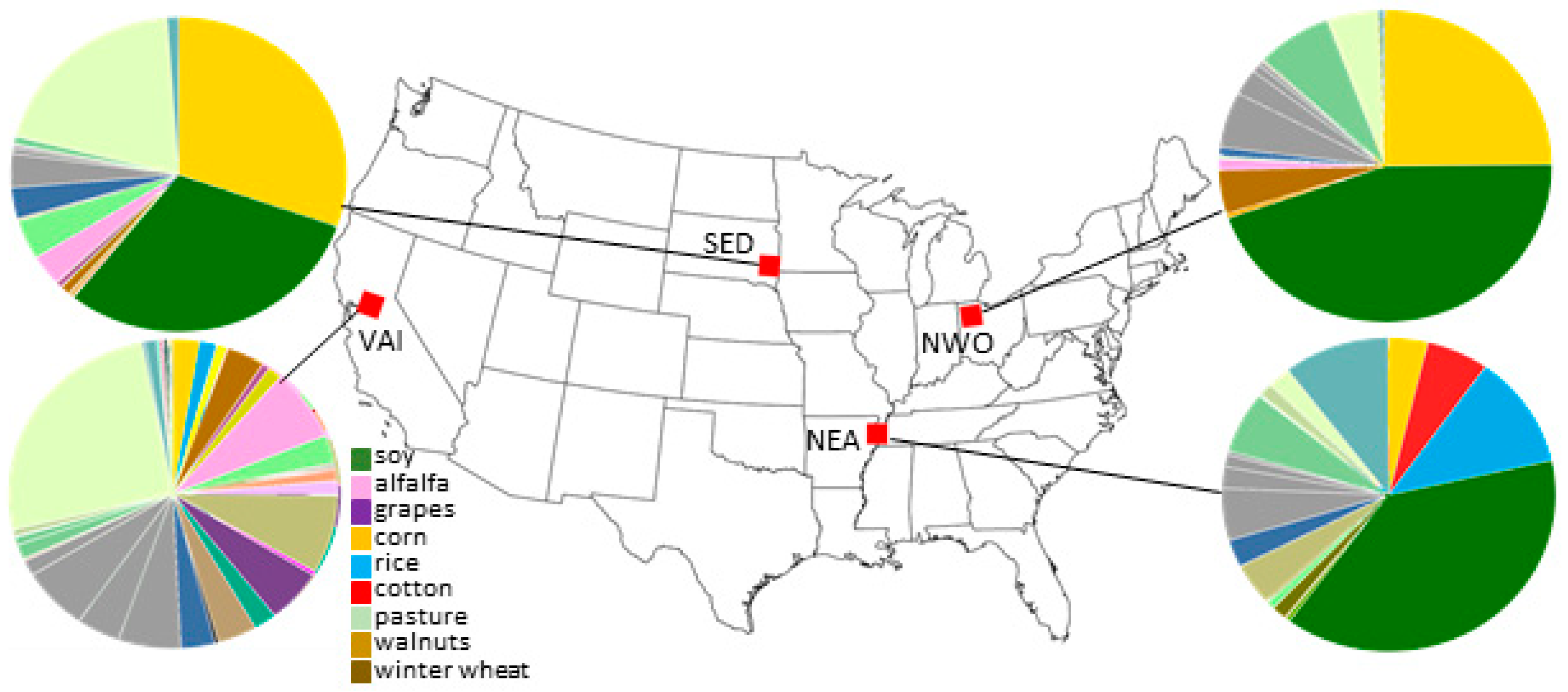
Four study regions approximately 110 × 110 km each were selected as case study sites (Figure 1). These regions were selected to represent major agricultural production hot spots in the USA with active field research that cover diverse bioclimates, soils, calendars, cloud probabilities, and management practices to provide a robust set of test landscapes. These included northwest Ohio (NWO), northeast Arkansas (NEA), southeast South Dakota (SED), and the northern Sacramento Valley, California (VAI). Major crops (>5% of landscape) in NWO and SED include corn, soybeans, winter wheat, and pasturelands. NEA includes cotton and rice production in addition to corn and soy. VAI has a diverse crop matrix with areas of grapes, tomatoes, corn, rice, alfalfa, sunflower, clover, almonds, and walnuts among other specialty crops (for example, onions, peas, watermelon, carrots). Rain season, crop calendars, and management practices vary within and among the study regions creating a robust set of calibration and validation crop type sites.
2.2. Sentinel-1 Processing
Dual polarization (VV + VH) Sentinel-1 Interferometric Wide (IW) Ground Range Detection (GRD) data were obtained from the Alaska Satellite Facility (ASF) for this application. Sentinel-1A carries a C-band imager at 5.405 GHz with an incidence angle between 20° and 45°. The platform follows a Sun-synchronous, near-polar, circular orbit at a height of 693 km. These C-band radar data were first transformed into Beta Naught to assist in radiometric terrain correction and thermal noise removal using the look-up table (LUT) within the metadata. Radiometric distortion caused by the terrain slope was corrected using the method proposed by Reference [16] to achieve Gamma Naught γ°, which is less dependent of the incidence angle than the Sigma Naught σ°. The inherent speckle noise was filtered using a Boxcar filter method with a 5-by-5 window size. Finally, with the assistance of the precise orbit and 30 m Shuttle Radar Topography Mission (SRTM) Digital Elevation Model (DEM), all data were geocoded using the range-Doppler approach with the output resolution of 30 by 30 m (to match a nominal application scale in this case). All radar preprocessing were executed using custom open access routines we built using Python, C, and GDAL and are available for sharing with author contact. At the time of this application, only Sentinel-1A was uniformly operational over these study domains.
2.3. Harmonized Landsat-8 Sentinel-2
The Harmonized Landsat-8 Sentinel-2 (HLS) is an ongoing processing chain effort to take advantage of widely accessible moderate resolution optical platforms to increase the potential number of temporal revisits (hls.gsfc.nasa.gov). This processing chain is evaluated over validation sites from AERosol RObotic NETwork, Fluxnet, Societal Applications in Fisheries & Aquaculture using Remotely Sensed Imagery, and Baseline Surface Radiation Network programs. The harmonization approach (1) grids imagery to a common pixel resolution, projection, and spatial extent (that is, tile); (2) applies atmospheric correction, the Landsat 8 Surface Reflectance Code (LaSRC) processor [17,18], relying of on a long heritage of Landsat processing; (3) applies LaSRC cloud masking using efficient cloud and cloud-shadow modules for Landsat-8 data [17,18] while Fmask [19] is used for Sentinel-2; (4) adjusts to represent the response from a common spectral bandpass and BRDF-normalization keying off a single, global and constant BRDF shape that produces satisfying BRDF normalization over a limited range of view zenith angle [20,21]; (5) perform geographic co-registration using the Automated Registration and Orthorectification Package (AROP) [22] to warp and co-register data. Note that the bandpass adjustment corresponds to a linear fit between the equivalent spectral bands. The regression coefficients were computed based on 500 hyperspectral spectra selected on 160 Hyperion scenes globally distributed. At the end of this harmonization processing chain, a temporal frequency of 1–3 days using synchronized platforms is achieved (hls.gsfc.nasa.gov). In this application reflectances, common indices (that is, NDVI, LSWI) that have shown value for classifying crops (that is, [23,24,25,26]) and thermal bands (TIR) were included as inputs into the classifier.
2.4. Classification and Assessment
Summarizing, S1, HLS, and blended HLS + S1 stacks were used in a hindcast approach (Figure 2, Table 1) to classify major crop types in the four case study regions. For a classifier, we used the ensemble, machine-learning, Random Forest (RF) algorithm [27]. Random forest is a flexible and powerful nonparametric technique that many mapping applications have recently implemented for a range of studies (for example, [28,29,30,31]). A random forest is generated through the creation of a series of classification/decision trees using bootstrapping, or resampling with replacement. Tuning parameters, such as the number of trees and the number of split candidate predictors, are generally chosen based on the out-of-bag (OOB) prediction error. In this application, we implement the random forest classifier from python sklearn and tuned with the exception of the number of trees.
The number of trees is set to a large number (200) because compared with other classifiers such as Support Vector Machine (SVM), the RF uses out-of-bag (OOB) samples for cross-validation, and once the OOB errors stabilize at a sufficiently large number of trees, the training can be concluded. The number of m variables that are selected randomly as candidates for splitting is set to the default which is the square root of the number of total input predictors p. It should be noted that when the number of variables p is large, but the fraction of relevant variables is small, RF can perform poorly with a small m. We further use a variable importance metric based on the Gini index, where predictors with higher importance are used more often to create a split, to understand how different days, sensors and bands relate to model performance, noting that varying scales of measurement between the predictors may also influence the importance ranking [32,33].
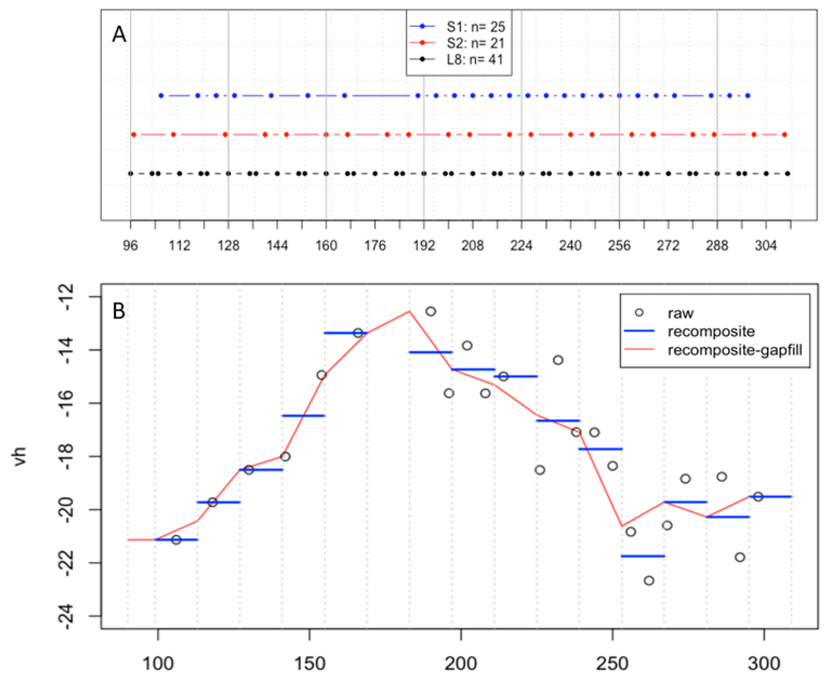
Due to the diverse imaging modes, acquisition dates, and the invalid values caused by cloud within HLS, we interpolated the images stacks to standardized 15-day time windows between the day of year 96 (6 April) and 308 (4 November). A 15-day interval was chosen to ensure at least one observation from each of the sensors was available in every time window and further supported by prior knowledge and subjective interpretation of plots (Figure 3). The interpolation was carried out using a multi-temporal time series routine that allows one to explore the temporal domain of a large space-time data set in an efficient manner. The routine, by reading small spatial chunks of all available time layers, carries out spatial location specific calculations on all-time layers grouped by time (that is, the year) and outputs maps of the time calculated values. Calculation algorithms are contained in separate modules that can be strung together in a user-specified step order for more complex calculations. In this application, we use a two-module step algorithm. It begins with a recomposite step, which calculates a band specific average for a 15-day window at each pixel and concludes with a gapfill step, which linearly interpolates the 15-day band specific average to fill in periods with no observations.
We qualitatively considered various options for smoothing (that is, References [34,35]) following the best practices and applications [36,37,38,39]. Ultimately, the focus of this work was blending the optical and radar data for crop type classification case study; thus, a linear interpolation was sufficient and simple to execute. If the first 15-day window was missing for a specific pixel and band, the spatial average of that band for all crop areas was used to fill the missing value. The multi-temporal processing for one single example pixel is shown in Figure 3. The advantage of this processing is an extremely efficient implementation and its flexibility to be used in a near real-time application since the approach gapfill interpolates using only past dates. Further investigation is needed to assess the uncertainties added by this approach, in particular, when few time points are available overall.
Crop type training and validation came from the 2016 USDA NASS CDL. Details on the creation of CDL can be found in Reference [40]. The CDL is a very good proxy for ground information because it provides pixel-level accuracies of around 95% for major commodities in intensively farmed regions (Table 2). For training, crop stratified random pixel (30 m resolution) samples of size 1000 in each of the four case study areas were selected from a sampling unit. Samples were restricted to homogenous patches of 5 by 5 windows with the same CDL class and pixels having at least five Landsat 8, three Sentinel 2 and five Sentinel 1 valid overpass dates during the crop season (DOY 96 to 308). The subsample locations were used to extract time series’ from multitemporal processed raster stacks of Harmonized Landsat and Sentinel 2 bands as well as Sentinel 1 bands VV and VH. Validation was carried out using all CDL major crop type pixels over each study area. Error matrices were generated based on these outcomes.
We further qualitatively assessed training data using a limited set of geofield photos taken during the crop season. These field-level “windshield drive-by” photos were collected using a smartphone app. All the geofield photos are linked to shape files or keyhole markup language (KML) files to store, display, and share photos. These photos are available for viewing and sharing at www.eomf.ou.edu/photos. Further, we used a limited set of Common Land Unit (CLU) polygons from the USDA Farm Service Agency to generate mean summary statistics from the integrated data stacks. These CLU data were also qualitatively used to compare training data statistically. Together, these ultimately provide high confidence in the use of the calibration and validation data.
3. Results
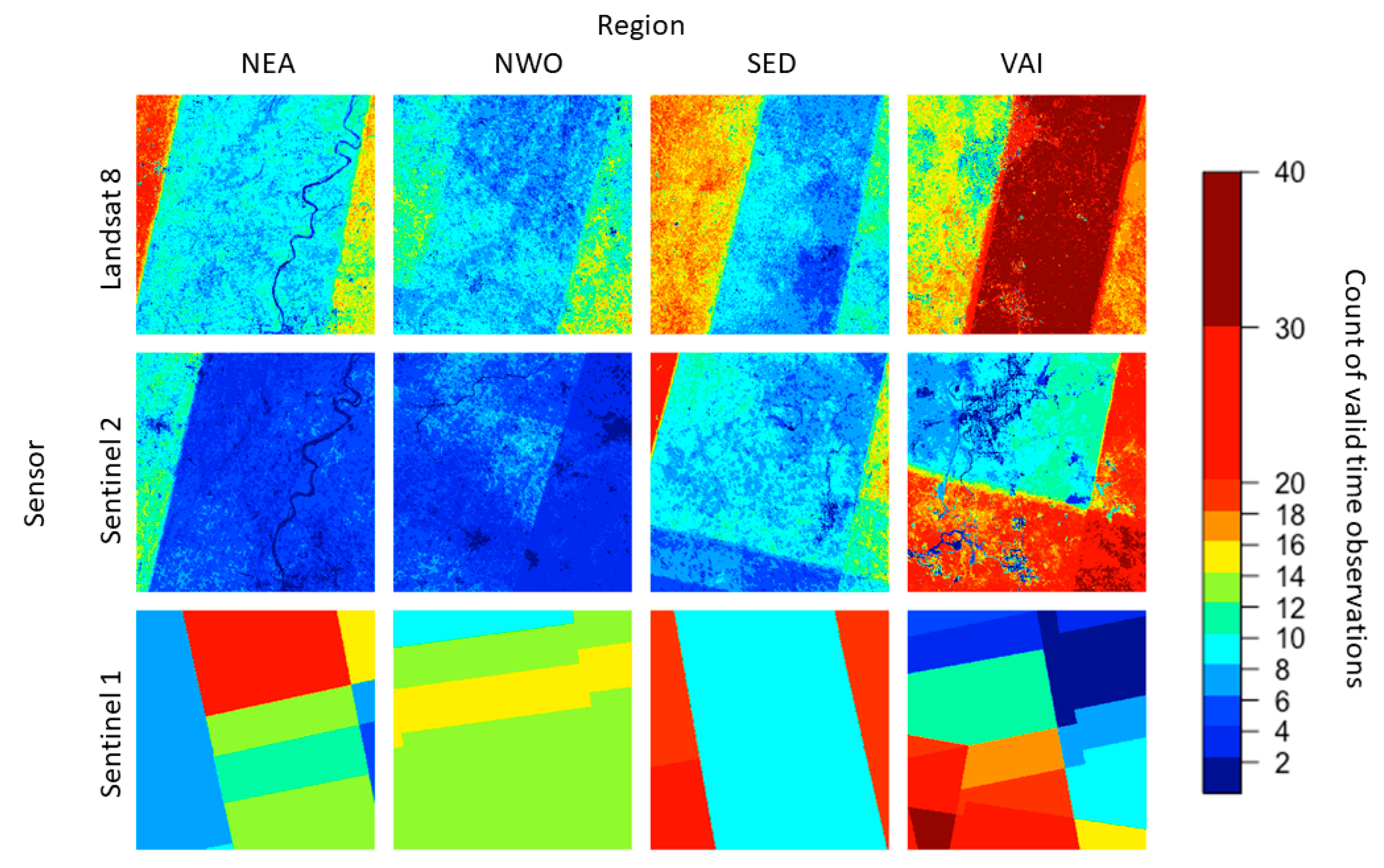
The cloud masks applied to the HLS imagery removed an average of 35, 37, 59, and 29% of valid pixels for NEA, NWO, SED, and VAI, respectively, across time (DOY 90–310) (Figure 4). Noted is that we did not perform regional tuning of the cloud mask algorithms given the operational context of this research application. The heat maps illustrating the number of quality observations shows that the valid counts range from 4–40 across the four case study sites. Further, the number of quality observations varies within the study regions due to the path row footprints, cloud, ascending versus descending orbits and the effects of the observations strategies. The highest frequency of observations is apparent in the path overlap regions.
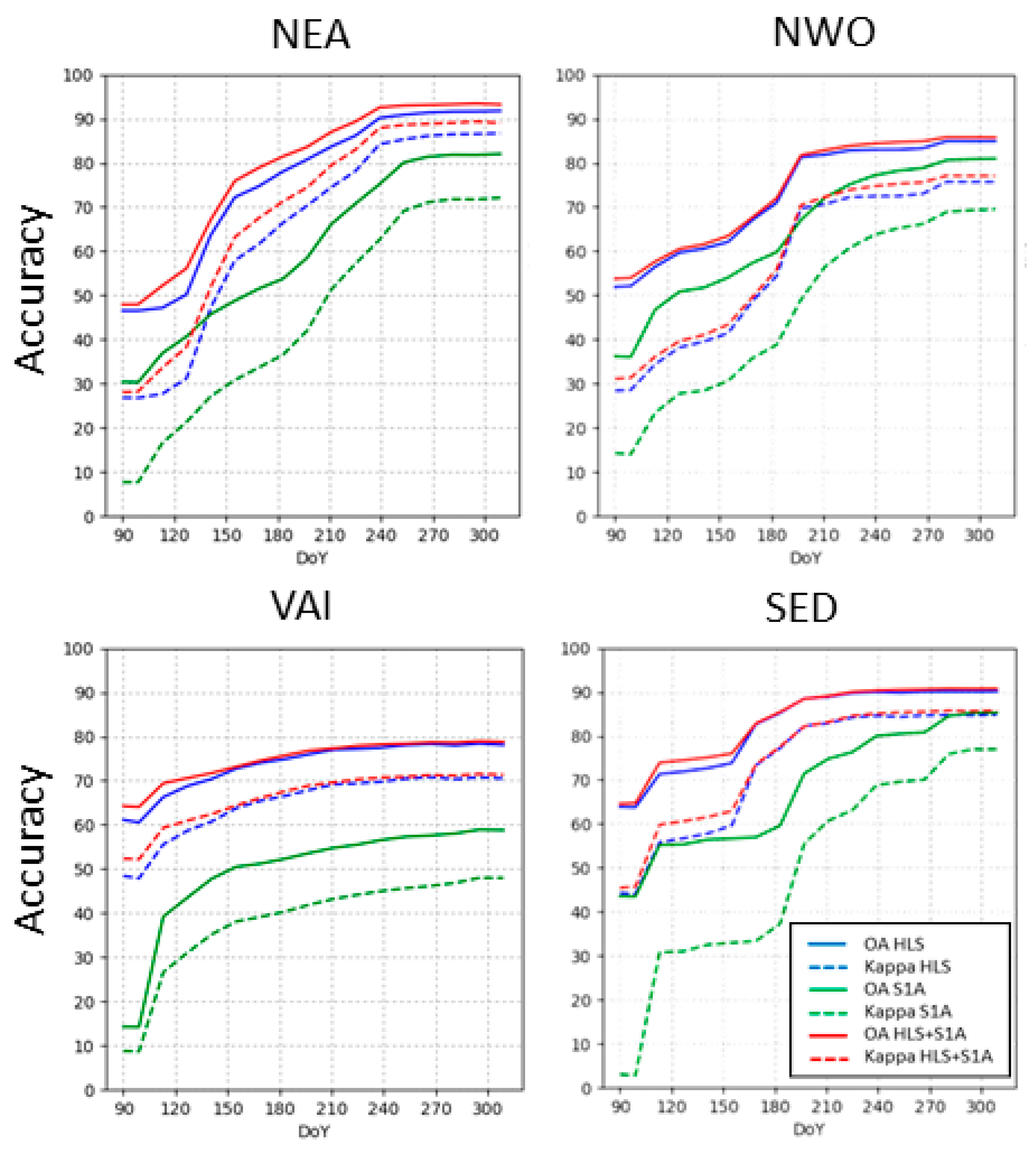
Accuracy measures range by region, sensor, time, and crop type. Note these error matrices reflect the model classes in that only major agricultural land uses were used (that is, no built, water, forested, and so forth), which, therefore, influences the accuracy and kappa outcomes. Using NEA (Figure 5) as an example, S1-only overall accuracies (OA) and kappa values for the first (DOY 96) period were 30% and 7, respectively, while the outcomes at the end of the season (DOY 300) were 82% and 72, respectively (Table 3). For HLS, the overall accuracies and kappa values for the first period were 47% and 27 while the outcomes at the end of the season were 92% and 87, respectively. For integrated stacks (HLS + S1) the overall and kappa outcomes were 48% and 28 initially while the end of the season values were 94% and 90, respectively.
Users and Producers Accuracies (UA/PA) for the first and end of season periods for NEA for major crops including corn, cotton, rice, and soybean are illustrated in Table 3. Corn had the most confusion with S1-only in NEA with UA of 52% by end of the season compared to 80% when using HLS. In VAI, almonds had an integrated UA of 27 and fallow cropland and winter wheat had UA slightly below 60% while all other crops had UA and PA over 60%, including corn, rice, alfalfa, tomatoes, grapes, grassland, and walnuts (Figure 6A,B). To succinctly summarize the hundreds of classifications (sensors × time × regions), Figure 7 summarizes the overall accuracy and kappa values for each site over time and by sensor type. Evident is the increasing accuracies as seasonal crops develop.
The variable importance was measured using the Gini index. Looking at the single highest Gini index by model, a given region typically maxes out using a certain variable (band) on a certain day of the year. These outcomes coincide with the overall accuracy and kappa plateaus for a given region. For NWO and SED, this is 197, while for NEA, this is 239 and in VAI it depends on the sensor (that is, HLS NDVI 113) or data availability. In VAI, there is a visible influence of data by sensor availability, which also factors in which bands have the highest Gini index. In VAI, NDVI, LSWI, and S2, the red edge-1 are intermixed over time as the highest ranked. In SED, NDVI followed by S2 red edge-1 show up as the most important from DOY 141 to 239. In NWO and NEA, LSWI, VV, and SWIR are ranked the highest. Cirrus and TIR were often ranked the least important across the four case study sites and over time.
4. Discussion
Generally, the HLS performed very well in these case studies of mapping major crop type in four US production hot spots. VAI with its 10 diverse crops was the only site which did not achieve >85% overall accuracy keeping in mind outcomes are relative (only major crop classes considered) and should be taken in the context of the study design. The S1 alone performed adequately while the combination of the radar and optical satellite imagery tended to out-perform any individual sensor earlier in the growing season. However, in many cases, the fusion of optical and radar only provide incremental improvements. For any given region, major crop, or time of year example arguments can be made of which sensor or combination is superior. We emphasize that this is a relatively simple case study testing ability to distinguish major crop types (categorical variable) only with the ensemble machine learning classifier.
We note that CDL was used as the primary calibration and validation data in this research application and this has inherent uncertainties. With the robust sampling approach described in combination with limited geofield photos and CLU considerations, we feel confident in the quality of the calibration and validation. The CDL PA and UA all have crop specific accuracies of over 93%, excluding corn, winter wheat, and pistachios in VAI. Therefore, it is possible these uncertainties influenced the outcomes of VAI. However, in our experience, CLUs, which are used to train CDL, have embedded errors and the misclassifications in CDL often tend to be related to noise (edge effect, speckling) so we suggest that this is as robust an overall approach as operationally feasible.
Clouds are often cited as the main advantage in using radar. Here the cloud masks generated with the HLS products were not further tuned and taken and applied as is. In the Southeast South Dakota study region, 38 HLS overpasses had more than 90% of the pixels flagged. It is very likely that these numbers could be lowed (improved) with regional tuning and cloud mask refinement. Masking clouds remains an evolving and active research topic [41,42]. However, the classification outcomes indicate the multitemporal routine, of compositing and interpolating the quality HLS observations, and the classification approach still out-performed the S1 only data by 5% and 8 for overall accuracy and kappa, respectively. Potentially, HLS in geographies like South or Southeast Asia with persistent clouds might be severely limited during crucial periods for food security decision making. These outcomes are also shaped by the study design and, in fact, only two bands are available from S1 IW mode (that is, VV, VH) versus several bands available from HLS and the use of random forest. It is possible that techniques leveraging quad polarization or repeat-pass interferometric information with more sensitivity tuned to the number and density, dielectric contrast, orientation and shape, or surface roughness of targets would improve radar only accuracy (for example, References [43,44]).
The timing of quality observations had an influence on the outcomes. The OA and kappa tend to plateau around DOY 200 for southeast Dakota and northwest Ohio with maximum accuracy leveling out. This is likely due to the relatively simple crop classification schemes of only corn, soy, and grasses (winter wheat and/or pasture). Northeast Arkansas did not plateau until DOY 240, and generally, S1 tended to plateau a few 15-day periods later than HLS, with the classifier using the additional observations to statistically differentiate between categories. This further amplifies the value of the additional parameters (bands) in terms of random forest computational needs. On the other hand, this approach allowed for a near real-time implementation.
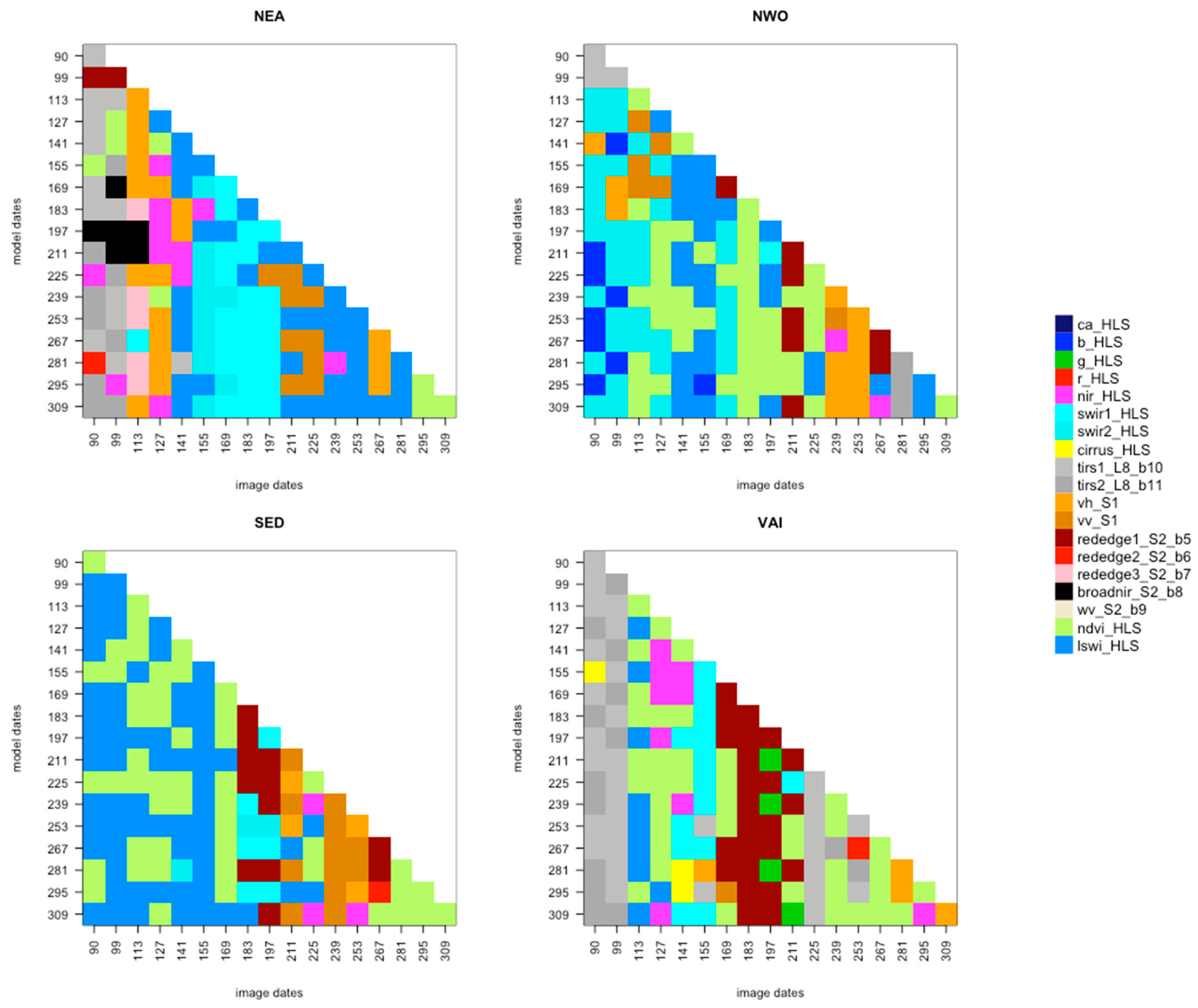
The timing and number observations are pronounced in the variable importance analysis. The ‘most valuable’ variable, according to this study context, can shift throughout the time series and does not necessarily have biogeophysical meaning tied to crop phenological attributes (for example, chlorophyll, biomass, leaf area index, roughness). Since we fit models iteratively in time there are complex interactions between the day of year and sensor band. In particular, the band with the highest Gini index for a particular image day input changes depending on the other dates available in the model. In Figure 8, we show this for each of the by-day NEA models when all HLS and S1A bands are included. For example, the band with the highest Gini index for the first image recomposite period (DOY 90) includes S2 Rededge-1, TIRS1, NIR, and NDVI. However, overall, the VH, LSWI, NIR, and SWIR bands populated the top variables during the key early season periods of crop development (Figure 8). This likely indicates that volume, leaf moisture or equivalent water thickness, green biomass vigor, and residue and organic matter are driving these parameters to the top of the classifier importance rankings. Parameters (bands) that showed up as the least important were cirrus and TIRS with the earlier periods (for example, DOY 90) getting the least weight.
5. Conclusions
Overall, the outcomes of these case study crop type classifications highlight the utility of higher temporal frequency moderate resolution data streams. Both HLS and S1 offer contributions to characterizing major crop types with the combination of radar and optical adding value (5–10% relative accuracy increases earlier and during the crop season). By the end of the crop season, the overall accuracy and kappa tend to converge showing equivalent capability in these regions. The harmonization of Landsat-8 and Sentinel-2 performed best and evident is the ability to distinguish major crop types within a season with high accuracy approaching harvest. Typically, observations from these sensors are available within 12–24 h providing a mechanism for near-real-time capabilities. However, it should be noted that currently HLS processing is not on demand and requires additional harmonization processing. In regions with chronic and persistent cloud cover, this work indicates Sentinel-1 can be very effective in providing major crop type inventory estimates within the season. With ESA striving for 24-h latency on S1 this should be able to support operational production. Given the short latency and quality calibration of these sensors, the science community is now beginning to take advantage of these opportunities to drive decision support tools and inventory programs to enhance food security with within season estimates of extent. Being able to monitor and assess production at field scale will drastically enhance decision making. Future work can consider evaluating fusion in other regions and crops, transferability of models across space and time (years), using additional ground truth for accuracy and uncertainty quantification, and scaling over large regions operationally are potential next steps. As more moderate resolution sensors come online in an operational context the agricultural monitoring community can potentially support within season major crop type production estimates. This can help to meet the most important need for food security.
Author Contributions
Conceptualization, N.T., B.Z., X.H.; Methodology, X.H., B.Z., N.T.; Data Curation, X.H., B.Z., J.M., D.J., M.R.; Writing, N.T.; Editing, N.T., B.Z., X.H., J.M., D.J., M.R.
Funding
This research was funded in part by NASA SBIR (S5.02-8891), NASA Earth Observations for Food Security and Agriculture Consortium (80NSSC17K0625), and NASA NISAR 17-009419A.
Acknowledgments
Thanks to Ian Cooke, Bobby Braswell, and Lindsey Melendy for assistance in data development, the HLS team at NASA Goddard Space Flight Center, ESA for Sentinel-1, the EOFSAC initiative and NASA-ISRO SAR Mission (NISAR), and data providers including NASA/USGS and ESA.
Conflicts of Interest
The authors declare no conflict of interest.
References
- Kussul, N.; Lavreniuk, M.; Skakun, S.; Shelestov, A. Deep Learning Classification of Land Cover and Crop Types Using Remote Sensing Data. IEEE Geosci. Remote Sens. Lett. 2017, 14, 778–782. [Google Scholar] [CrossRef]
- Whitcraft, A.; Becker-Reshef, I.; Justice, C. Agricultural growing season calendars derived from MODIS surface reflectance. Int. J. Digit. Earth 2014, 8, 173–197. [Google Scholar] [CrossRef]
- Becker-Reshef, I.; Vermote, E.; Lindeman, M.; Justice, C. A Generalized Regression-based Model for Forecasting Winter Wheat Yields in Kansas and Ukraine Using MODIS Data. Remote Sens. Environ. 2010, 114, 1312–1323. [Google Scholar] [CrossRef]
- Franch, B.; Vermote, E.; Becker-Reshef, I.; Claverie, M.; Huang, J.; Zhang, J.; Justice, C.; Sobrino, J. Improving the timeliness of winter wheat production forecast in the United States of America, Ukraine and China using MODIS data and NCAR Growing Degree Day information. Remote Sens. Environ. 2015, 161, 131–148. [Google Scholar] [CrossRef]
- Johnson, D. A comprehensive assessment of the correlations between field crop yields and commonly used MODIS products. Int. J. Appl. Earth Obs. Geoinform. 2016, 52, 65–81. [Google Scholar] [CrossRef] [Green Version]
- Xiong, J.; Thenkabail, P.S.; Tilton, J.C.; Gumma, M.K.; Teluguntla, P.; Oliphant, A. Nominal 30-m Cropland Extent Map of Continental Africa by Integrating Pixel-Based and Object-Based Algorithms Using Sentinel-2 and Landsat-8 Data on Google. Remote Sens. 2017, 9, 1065. [Google Scholar] [CrossRef]
- Song, X.P.; Potapov, P.V.; Krylov, A.; King, L.; Di Bella, C.M.; Hudson, A.; Khan, A.; Adusei, B.; Stehman, S.V.; Hansen, M.C. National-scale soybean mapping and area estimation in the United States using medium resolution satellite imagery and field survey. Remote Sens. Environ. 2017, 190, 383–395. [Google Scholar] [CrossRef]
- McNairn, H.; Champagne, C.; Shang, J.; Holmstrom, D.; Reichert, G. Integration of optical and Synthetic Aperture Radar (SAR) imagery for delivering operational annual crop inventories. Int J. Photogramm. Remote Sens. 2009, 64, 434–449. [Google Scholar] [CrossRef]
- Bouvet, A.; LeToan, T.; Lam-Dao, N. Monitoring of the rice cropping system in the Mekong Delta using ENVISAT/ASAR dual polarization data. IEEE Trans. Geosci. Remote Sens. 2011, 47, 517–526. [Google Scholar] [CrossRef] [Green Version]
- Liao, C.; Wang, J.; Shang, J.; Huang, X.; Liu, J.; Huffman, T. Sensitivity study of Radarsat-2 polarimetric SAR to crop height and fractional vegetation cover of corn and wheat. Int. J. Remote Sens. 2018, 39, 1475–1490. [Google Scholar] [CrossRef]
- Huang, X.; Wang, J.; Shang, J.; Liao, C.; Liu, J. Application of polarization signature to land cover scattering mechanism analysis and classification using multi-temporal C-band polarimetric RADARSAT-2 imagery. Remote Sens. Environ. 2018, 193, 11–28. [Google Scholar] [CrossRef]
- Torbick, N.; Chowdhury, D.; Salas, W.; Qi, J. Monitoring rice agriculture across Myanmar using time series Sentinel-1 assisted by Landsat-8 and PALSAR-2. Remote Sens. 2017, 9, 119. [Google Scholar] [CrossRef]
- Clauss, K.; Ottinger, M.; Kuenzer, C. Mapping rice areas with Sentinel-1 time series and superpixel segmentation. Int. J. Remote Sens. 2018, 39, 1399–1420. [Google Scholar] [CrossRef]
- Nelson, A.; Setiyono, T.; Rala, A.B.; Quicho, E.D.; Raviz, J.V.; Abonete, P.J.; Maunahan, A.A.; Garcia, C.A.; Bhatti, H.Z.M.; Villano, L.S.; et al. Towards an Operational SAR-Based Rice Monitoring System in Asia: Examples from 13 Demonstration Sites across Asia in the RIICE Project. Remote Sens. 2014, 6, 10773–10812. [Google Scholar] [CrossRef] [Green Version]
- Steventon, M.; Ward, S.; Dyke, G.; Sobue, S.; Oyoshi, K. Asian Rice Crop Estimation and Monitoring Component of GEOGLAM (Asia-RiCE) 2017/Phase 2 Implementation Report; JAXA (Japan Aerospace Exploration Agency): Tokyo, Japan, 2018. [Google Scholar]
- Small, D. Flattening Gamma: Radiometric Terrain Correction for SAR Imagery. IEEE Trans. Geosci. Remote Sens. 2011, 49, 3081–3093. [Google Scholar] [CrossRef]
- Vermote, E.; Justice, C.; Claverie, M.; Franch, B. Preliminary analysis of the performance of the Landsat 8/OLI land surface reflectance product. Remote Sens. Environ. 2016, 185, 46–56. [Google Scholar] [CrossRef]
- Masek, J.G.; Vermote, E.F.; Saleous, N.E.; Wolfe, R.; Hall, F.G.; Huemmrich, K.F.; Gao, F.; Kutler, J.; Lim, T.K. A Landsat surface reflectance dataset for North America, 1990–2000. IEEE Geosci. Remote Sens. Soc. 2006, 3, 68–72. [Google Scholar] [CrossRef]
- Zhu, Z.; Wang, S.; Woodcock, C.E. Improvement and expansion of the Fmask algorithm: Cloud, cloud shadow, and snow detection for Landsats 4-7, 8, and Sentinel 2 images. Remote Sens. Environ. 2015, 159, 269–277. [Google Scholar] [CrossRef]
- Claverie, M.; Vermote, E.; Franch, B.; He, T.; Hagolle, O.; Kadiri, M.; Masek, J. Evaluation of Medium Spatial Resolution BRDF-Adjustment Techniques Using Multi-Angular SPOT4 (Take5) Acquisitions. Remote Sens. 2015, 7, 12057–12075. [Google Scholar] [CrossRef]
- Roy, D.P.; Zhang, H.K.; Ju, J.; Gomez-Dans, J.L.; Lewis, P.E.; Schaaf, C.B.; Sun, Q.; Li, J.; Huang, H.; Kovalskyy, V. A general method to normalize Landsat reflectance data to nadir BRDF adjusted reflectance. Remote Sens. Environ. 2016, 176, 255–271. [Google Scholar] [CrossRef]
- Gao, F.; Masek, J.G.; Wolfe, R.E. Automated registration and orthorectification package for Landsat and Landsat-like data processing. J. Appl. Remote Sens. 2009, 3, 033515. [Google Scholar]
- Rouse, J.W.; Haas, R.H.; Schell, J.A.; Deering, D.W. Monitoring vegetation systems in the Great Plains with ERTS. In Proceedings of the Third ERTS Symposium, Washington, DC, USA, 10 December 1974. [Google Scholar]
- Tucker, C.J. Red and photographic infrared linear combinations for monitoring vegetation. Remote Sens. Environ. 1979, 8, 127–150. [Google Scholar] [CrossRef] [Green Version]
- Xiao, X.; Boles, S.; Liu, J.; Zhuang, D.; Liu, M. Characterization of forest types in Northeastern China, using multi-temporal SPOT-4 VEGETATION sensor data. Remote Sens. Environ. 2002, 82, 335–348. [Google Scholar] [CrossRef] [Green Version]
- Hagen, S.; Heilman, P.; Marsett, R.; Torbick, N.; Salas, W.; van Ravensway, J.; Qi, J. Mapping total vegetation cover across western rangelands with MODIS data. Rangel. Ecol. Manag. 2012, 65, 456–467. [Google Scholar] [CrossRef]
- Breiman, L. Random Forests. Mach. Learn. 2001, 45, 5–32. [Google Scholar] [CrossRef] [Green Version]
- Wilkes, P.; Jones, S.D.; Suarez, L.; Mellor, A.; Woodgate, W.; Soto-Berelov, M.; Haywood, A.; Skidmore, A.K. Mapping forest canopy height over large areas by upscaling ALS estimates with freely available satellite data. Remote Sens. 2015, 7, 12563–12587. [Google Scholar] [CrossRef]
- Song, W.; Dolon, J.M.; Cline, D.; Xiong, G. Leanring-based algal bloom event recognition for oceanographic decision support system using remote sensing data. Remote Sens. 2015, 7, 13564–13585. [Google Scholar] [CrossRef]
- Torbick, N.; Corbiere, M. Mapping urban sprawl and impervious surfaces in the northeast United States for the past four decades. GISci. Remote Sens. 2015, 52, 746–764. [Google Scholar] [CrossRef]
- Karlson, M.; Ostwald, M.; Reese, H.; Sanou, J.; Tankoano, B.; Mattsson, E. Mapping tree canopy cover and aboveground biomass in Sudano-Sahelian woodlands using Landsat 8 and random forest. Remote Sens. 2015, 7, 10017–10041. [Google Scholar] [CrossRef]
- Hastie, T.; Tibshirani, R.; Friedman, J.H. The Elements of Statistical Learning: Data Mining, Inference, and Prediction, 2nd ed.; Springer: New York, NY, USA, 2009. [Google Scholar]
- Strobl, C.; Boulesteix, A.-L.; Zeileis, A.; Hothorn, T. Bias in random forest variable importance measures: Illustrations, sources and a solution. BMC Bioinform. 2007, 8, 25. [Google Scholar] [CrossRef] [PubMed] [Green Version]
- Savitzky, A.; Golay, M.J.E. Smoothing and Differentiation of Data by Simplified Least Squares Procedures. Anal. Chem. 1964, 36, 1627–1639. [Google Scholar] [CrossRef]
- Whittaker, E.T.; Robinson, G. The Calculus of Observations. Trans. Fac. Act. 1924, 10, 1924–1925. [Google Scholar]
- Atzberger, C.; Eilers, P.H.C. A time series for monitoring vegetation activity and phenology at 10-daily time steps covering large parts of South America. Int. J. Dig. Earth 2011, 4, 365–386. [Google Scholar] [CrossRef]
- Atkinson, P.M.; Jeganathan, C.; Dash, J.; Atzberger, C. Inter-comparison of four models for smoothing satellite sensor time-series data to estimate vegetation phenology. Remote Sens. Environ. 2012, 123, 400–417. [Google Scholar] [CrossRef]
- Eilers, P.H.C. A Perfect Smoother. Anal. Chem. 2003, 75, 3631–3636. [Google Scholar] [CrossRef] [PubMed]
- Jönsson, P.; Eklundh, L. TIMESAT—A program for analyzing time-series of satellite sensor data. Comput. Geosci. Vol. 2004, 30, 833–845. [Google Scholar] [CrossRef]
- Boryan, C.; Yang, Z.; Mueller, R.; Craig, M. Monitoring US agriculture: The US Department of Agriculture, National Agricultural Statistics Service, Cropland Data Layer Program. Geocarto Int. 2011, 26, 341–358. [Google Scholar] [CrossRef]
- Foga, S.; Scaramuzza, P.; Guo, S.; Zhu, Z.; Dilley, R.; Beckmann, T.; Schmidt, G.; Dwyer, J.; Hughes, M.; Laue, B. Cloud detection algorithm comparison and validation for operational Landsat data products. Remote Sens. Environ. Vol. 2017, 194, 379–390. [Google Scholar] [CrossRef] [Green Version]
- Qiu, S.; He, B.; Zhu, Z.; Quan, X. Improving Fmask cloud and cloud shadow detection in mountainous area for Landsats 4–8 images. Remote Sens. Environ. 2017, 199, 107–119. [Google Scholar] [CrossRef]
- Huang, X.; Wang, J.; Shang, J. An integrated surface parameter inversion scheme over agricultural fields at early growing stages by means of C-band polarimetric RADARSAT-2 imagery. IEEE Trans. Geosci. Remote Sens. 2017, 54, 2510–2528. [Google Scholar] [CrossRef]
- Canisius, F.; Shang, J.; Liu, J.; Huang, X.; Ma, B.; Jiao, X.; Geng, X.; Kovacs, J.; Walters, D. Tracking crop phenological development using multi-temporal polarimetric Radarsat-2 data. Remote Sens. Environ. Vol. 2018, 210, 508–518. [Google Scholar] [CrossRef]
Figure 1.
The four diverse case study sites located in major production hot spots in the USA with varying bioclimates, calendars, and managements.
Figure 1.
The four diverse case study sites located in major production hot spots in the USA with varying bioclimates, calendars, and managements.

Figure 2.
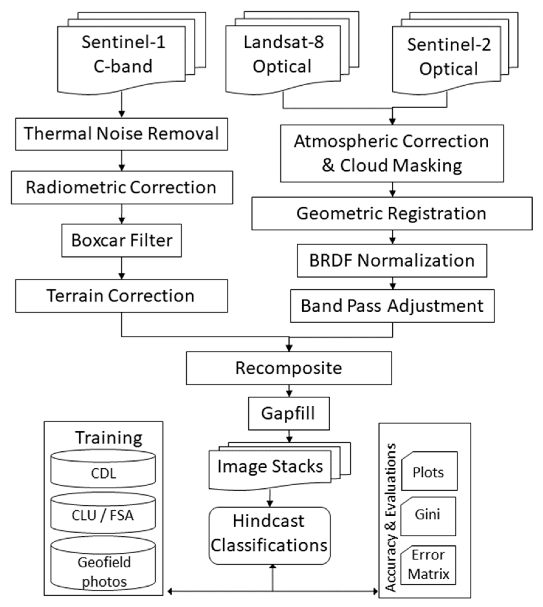
The conceptual workflow fusing multitemporal radar and optical moderate resolution imagery.
Figure 2.
The conceptual workflow fusing multitemporal radar and optical moderate resolution imagery.

Figure 3.
An example (A) time-frequency collected by sensor type across the northeast Arkansas (NEA) case study region. An example (B) multitemporal time series routine post processing Sentinel-1 VH observations a single corn pixel from NEA. Open circles (raw) give the VH backscatter γ° from the original image overpass date (2016). Blue lines (recomposite) are the mean value for each 15-day window shown by the vertical gray dotted lines, and the red line illustrates the final smoothed/interpolated classification inputs.

Figure 4.
The heat maps by sensor and region showing cloud masked observation frequency.

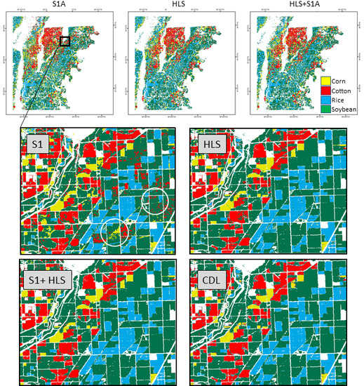
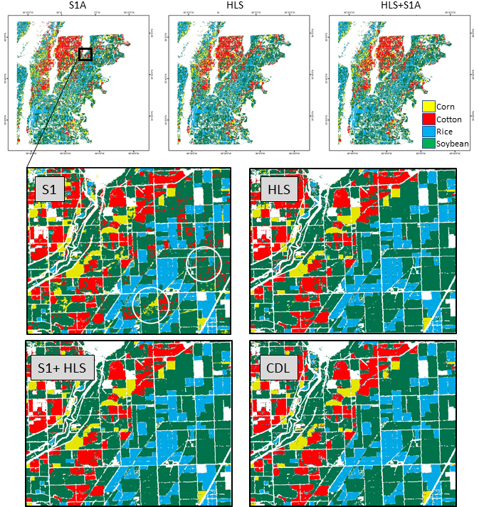
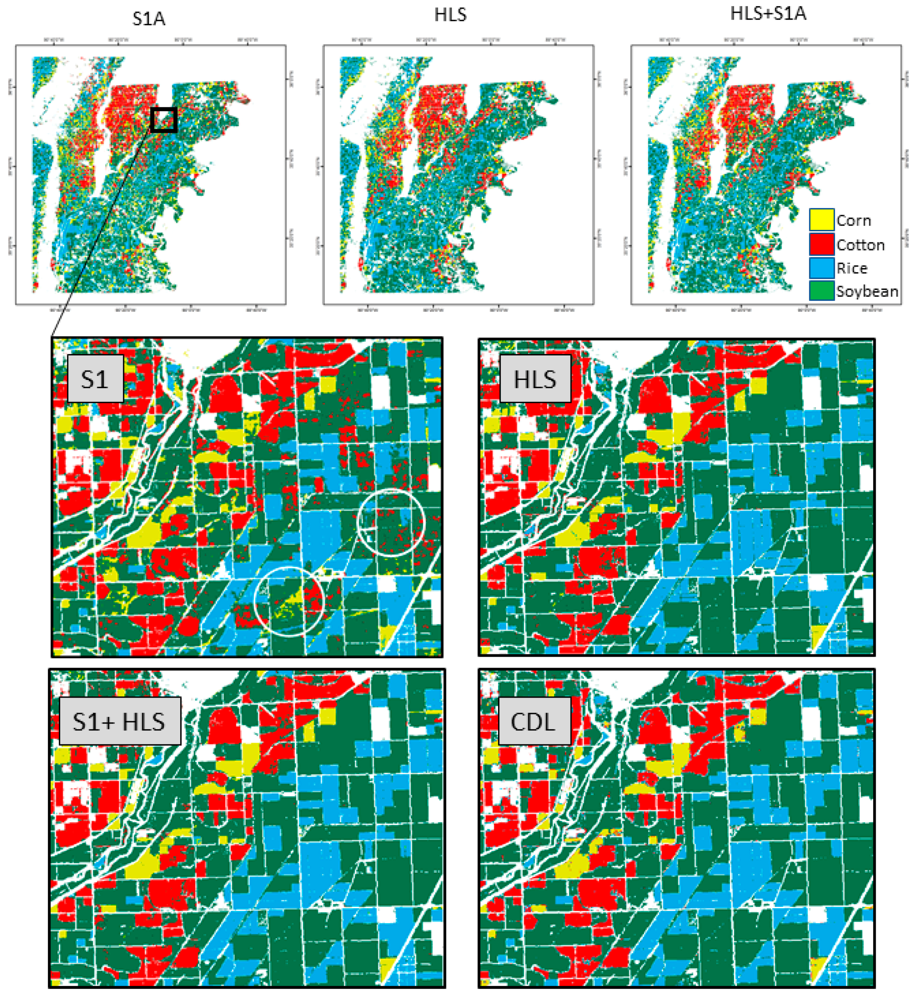
Figure 5.
Example end of season crop type classification maps in northeast Arkansas by sensors showing a generally strong ability to map major crop type within season at the field scale. The highlighted are example S1 that are only misclassification among corn, soy, and cotton.
Figure 5.
Example end of season crop type classification maps in northeast Arkansas by sensors showing a generally strong ability to map major crop type within season at the field scale. The highlighted are example S1 that are only misclassification among corn, soy, and cotton.

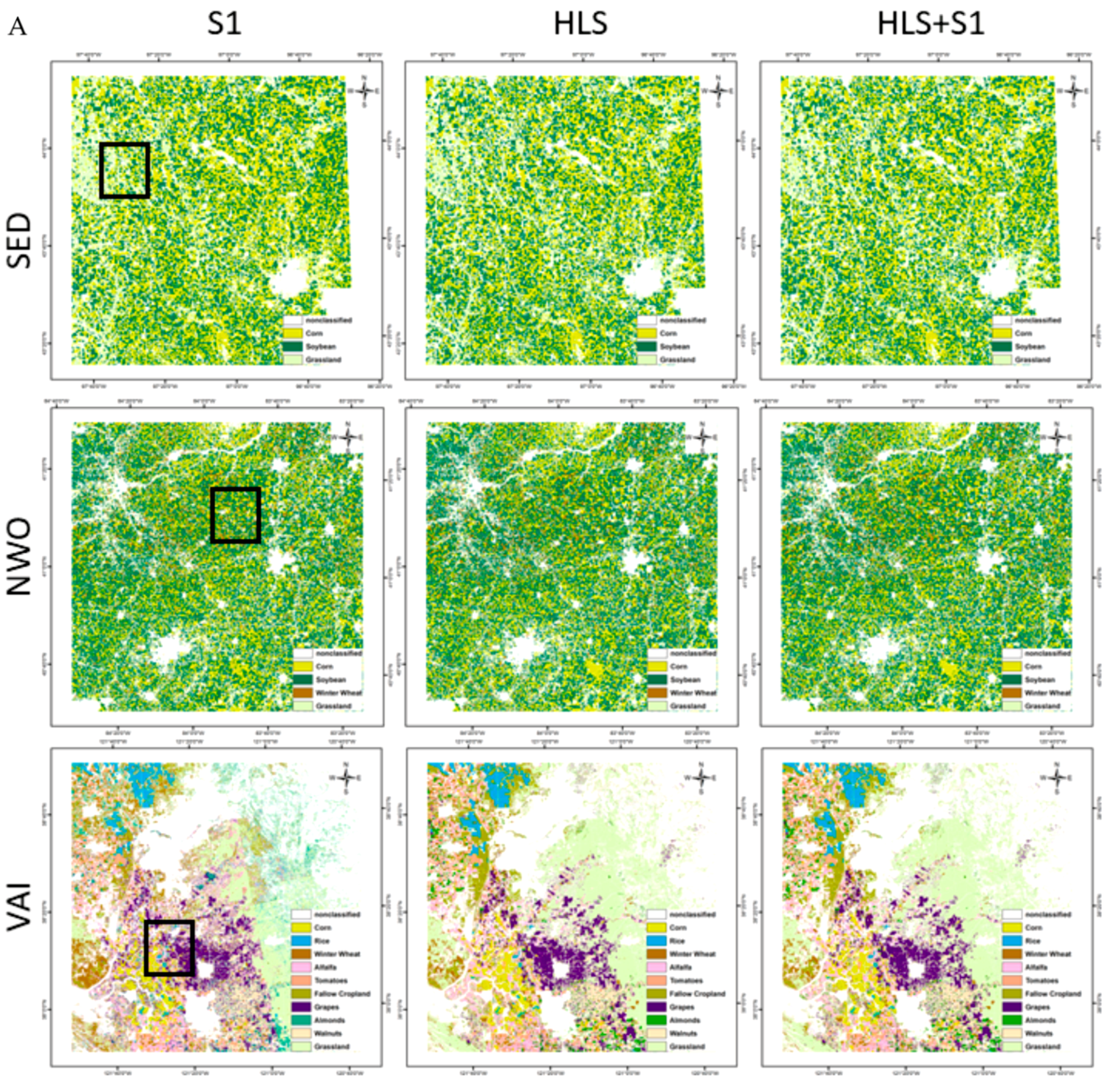
Figure 6.
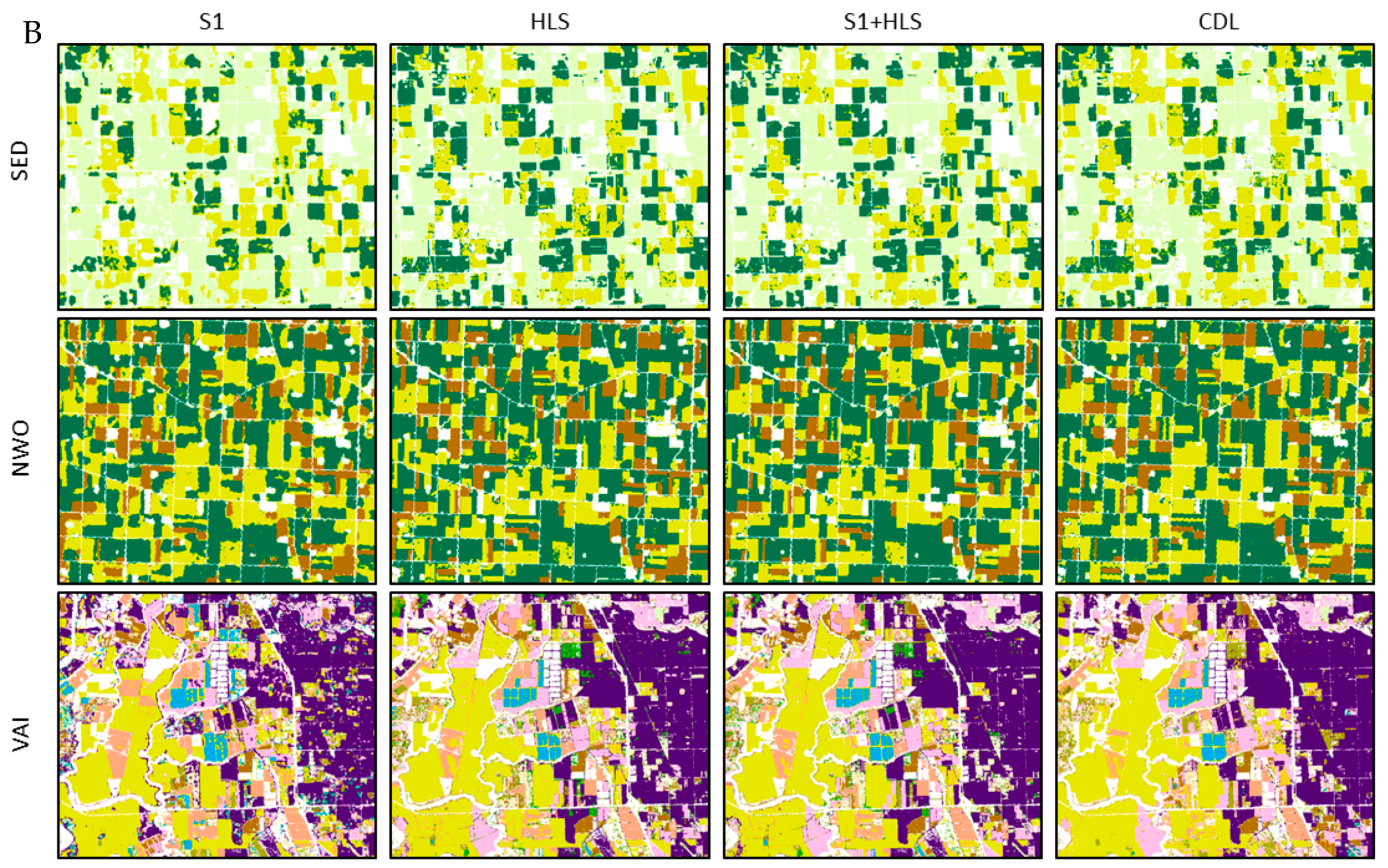
(A) The end of season crop type products for northwest Ohio, southeast South Dakota, and Sacramento Valley California by sensor type and combination; zoom-in continued on (B). (B) Representative zoomed in snapshots from (A), the end of season crop type products for southeast South Dakota, northwest Ohio, and Sacramento Valley California by sensor type and combination.
Figure 6.
(A) The end of season crop type products for northwest Ohio, southeast South Dakota, and Sacramento Valley California by sensor type and combination; zoom-in continued on (B). (B) Representative zoomed in snapshots from (A), the end of season crop type products for southeast South Dakota, northwest Ohio, and Sacramento Valley California by sensor type and combination.


Figure 7.
The overall accuracy and kappa values by sensor types over the crop season in the four case study regions.
Figure 7.
The overall accuracy and kappa values by sensor types over the crop season in the four case study regions.

Figure 8.
The summary of the highest ranked parameter (band) across the four case study regions over time. For example, on DOY 127 following bands can be seen as highest ranked for the given regions: NEA VH and NIR-HLS; NWO SWIR1-HLS, NDVI-HLS, and VV; SED NDVI-HLS and LSWI-HLS; and VAI NIR-HLS, NDVI-HLS, and LSWI-HLS.


Table 1.
The moderate resolution Earth observation inputs for crop classifier.
| Sensors | Band Code | Band Name | Wavelength (Micrometers) |
|---|---|---|---|
| HLS | CA | Coastal Aerosol | 0.44 |
| B | Blue | 0.48 | |
| G | Green | 0.56 | |
| R | Red | 0.66 | |
| NIR | NIR Narrow | 0.86 | |
| SWIR1 | SWIR1 | 1.61 | |
| SWIR2 | SWIR2 | 2.2 | |
| CIRRUS | Cirrus | 1.37 | |
| NDVI | Normalized Difference Vegetation Index-(NIR-R)/(NIR + R) | Index | |
| LSWI | Land Surface Water Index-(NIR-SWIR1)/(NIR + SWIR1) | Index | |
| Landsat-8 | TIRS1 | Thermal Infrared 1 | 10.90 |
| TIRS2 | Thermal Infrared 2 | 12.00 | |
| Sentinel-2 | REDEDGE1 | Vegetation Red Edge 1 | 0.71 |
| REDEDGE2 | Vegetation Red Edge 2 | 0.74 | |
| REDEDGE3 | Vegetation Red Edge 3 | 0.78 | |
| BROADNIR | Broad NIR | 0.84 | |
| WV | Water Vapor | 0.95 | |
| Sentinel-1 | VH | VH polarization | C-band |
| VV | VV polarization | C-band |
Table 2.
The cropland data layer accuracies statistics for major crops across four case study regions.
Table 2.
The cropland data layer accuracies statistics for major crops across four case study regions.
| Producers Accuracy | Omission Error | Kappa | Users Accuracy | Commission Error | Conditional Kappa | |
|---|---|---|---|---|---|---|
| NEA | ||||||
| Corn | 94.63 | 5.37 | 0.94 | 96.00 | 4.00 | 0.96 |
| Cotton | 94.37 | 5.63 | 0.94 | 97.07 | 2.93 | 0.97 |
| Rice | 97.49 | 2.51 | 0.97 | 98.20 | 1.80 | 0.98 |
| Soybeans | 97.34 | 2.66 | 0.96 | 94.35 | 5.65 | 0.92 |
| NWO | ||||||
| Corn | 97.30 | 2.70 | 0.96 | 97.70 | 2.30 | 0.97 |
| Soybeans | 97.98 | 2.02 | 0.97 | 98.08 | 1.92 | 0.97 |
| Winter wheat | 97.29 | 2.71 | 0.97 | 94.09 | 5.91 | 0.94 |
| SED | ||||||
| Corn | 96.77 | 3.23 | 0.96 | 96.01 | 3.99 | 0.95 |
| Soybeans | 97.05 | 2.95 | 0.96 | 96.12 | 3.88 | 0.95 |
| Winter wheat | 94.92 | 5.08 | 0.95 | 96.04 | 3.96 | 0.96 |
| VAI | ||||||
| Corn | 85.85 | 14.15 | 0.86 | 92.68 | 7.32 | 0.93 |
| Cotton | 98.04 | 1.96 | 0.98 | 94.88 | 5.12 | 0.95 |
| Rice | 99.77 | 0.23 | 1.00 | 99.89 | 0.11 | 1.00 |
| Winter wheat | 83.03 | 16.97 | 0.82 | 86.43 | 13.57 | 0.86 |
| Alfalfa | 96.25 | 3.75 | 0.96 | 93.34 | 6.66 | 0.93 |
| Tomatoes | 94.32 | 5.68 | 0.94 | 94.89 | 5.11 | 0.95 |
| Grapes | 92.24 | 7.76 | 0.92 | 92.27 | 7.73 | 0.92 |
| Almonds | 92.24 | 7.06 | 0.93 | 92.57 | 7.43 | 0.92 |
| Pistachios | 83.79 | 16.21 | 0.83 | 89.90 | 10.10 | 0.90 |
Table 3.
An example error matrix for one classification scheme in northeast Arkansas (NEA) by sensor combinations at Day Of Year 96 and 300 highlighting shifts in accuracy.
Table 3.
An example error matrix for one classification scheme in northeast Arkansas (NEA) by sensor combinations at Day Of Year 96 and 300 highlighting shifts in accuracy.
| Integrated (HLS + S1) | Harmonized Landsat-8 Senstinel-2 | Sentinel-1 | |||||||||||||||||||
| Corn | Cotton | Rice | Soybean | Total | UA (%) | Corn | Cotton | Rice | Soybean | Total | UA (%) | Corn | Cotton | Rice | Soybean | Total | UA (%) | ||||
| Time period 1 (DOY 96) | Corn | 264,005 | 118,443 | 183,718 | 433,604 | 999,770 | 26.4 | Corn | 270,040 | 131,110 | 194,874 | 470,155 | 1,066,179 | 25.3 | Corn | 62,610 | 119,855 | 110,135 | 348,240 | 640,840 | 9.8 |
| Cotton | 81,110 | 483,831 | 135,953 | 614,877 | 1,315,771 | 36.8 | Cotton | 79,956 | 471,564 | 135,803 | 599,531 | 1,286,854 | 36.6 | Cotton | 74,351 | 239,036 | 146,220 | 611,790 | 1,071,397 | 22.3 | |
| Rice | 29,982 | 31,396 | 570,107 | 706,372 | 1,337,857 | 42.6 | Rice | 29,839 | 36,314 | 568,741 | 751,340 | 1,386,234 | 41.0 | Rice | 235,002 | 227,251 | 709,842 | 1,406,737 | 2,578,832 | 27.5 | |
| Soybean | 58,762 | 107,978 | 227,970 | 1,196,236 | 1,590,946 | 75.2 | Soybean | 54,024 | 102,660 | 218,330 | 1,130,063 | 1,505,077 | 75.1 | Soybean | 61,896 | 155,506 | 151,551 | 584,322 | 953,275 | 61.3 | |
| Total | 433,859 | 741,648 | 1,117,748 | 2,951,089 | 5,244,344 | Total | 433,859 | 741,648 | 1,117,748 | 2,951,089 | 5,244,344 | Total | 433,859 | 741,648 | 1,117,748 | 2,951,089 | 5,244,344 | ||||
| PA (%) | 60.9 | 65.2 | 51.0 | 40.5 | PA (%) | 62.2 | 63.6 | 50.9 | 38.3 | PA (%) | 14.4 | 32.2 | 63.5 | 19.8 | |||||||
| OA (%) | 47.9 | OA (%) | 46.5 | OA (%) | 30.4 | ||||||||||||||||
| Kappa (%) | 28.1 | Kappa (%) | 26.8 | Kappa (%) | 7.7 | ||||||||||||||||
| Corn | Cotton | Rice | Soybean | Total | UA (%) | Corn | Cotton | Rice | Soybean | Total | UA (%) | Corn | Cotton | Rice | Soybean | Total | UA (%) | ||||
| Time period 17 (DOY 300) | Corn | 420,581 | 19,979 | 30,536 | 49,914 | 521,010 | 80.7 | Corn | 420,014 | 20,027 | 33,408 | 54,074 | 527,523 | 79.6 | Corn | 388,786 | 21,376 | 77,938 | 261,976 | 750,076 | 51.8 |
| Cotton | 1146 | 672,896 | 32,378 | 67,362 | 773,782 | 87.0 | Cotton | 1061 | 665,961 | 34,998 | 90,957 | 792,977 | 84.0 | Cotton | 5570 | 609,824 | 27,540 | 188,674 | 831,608 | 73.3 | |
| Rice | 2406 | 4438 | 1,000,419 | 38,225 | 1,045,488 | 95.7 | Rice | 4380 | 5519 | 990,093 | 69,757 | 1,069,749 | 92.6 | Rice | 14,371 | 6838 | 924,401 | 120,871 | 1,066,481 | 86.7 | |
| Soybean | 9726 | 44,335 | 54,415 | 2,795,588 | 2,904,064 | 96.3 | Soybean | 8404 | 50,141 | 59,249 | 2,736,301 | 2,854,095 | 95.9 | Soybean | 25,132 | 103,610 | 87,869 | 2,379,568 | 2,596,179 | 91.7 | |
| Total | 433,859 | 741,648 | 1,117,748 | 2,951,089 | 5,244,344 | Total | 433,859 | 741,648 | 1,117,748 | 2,951,089 | 5,244,344 | Total | 433,859 | 741,648 | 1,117,748 | 2,951,089 | 5,244,344 | ||||
| PA (%) | 96.9 | 90.7 | 89.5 | 94.7 | PA (%) | 96.8 | 89.8 | 88.6 | 92.7 | PA (%) | 89.6 | 82.2 | 82.7 | 80.6 | |||||||
| OA (%) | 93.2 | OA (%) | 91.8 | OA (%) | 82.0 | ||||||||||||||||
| Kappa (%) | 89.0 | Kappa (%) | 86.7 | Kappa (%) | 72.1 | ||||||||||||||||
© 2018 by the authors. Licensee MDPI, Basel, Switzerland. This article is an open access article distributed under the terms and conditions of the Creative Commons Attribution (CC BY) license (http://creativecommons.org/licenses/by/4.0/).
Share and Cite
MDPI and ACS Style
Torbick, N.; Huang, X.; Ziniti, B.; Johnson, D.; Masek, J.; Reba, M. Fusion of Moderate Resolution Earth Observations for Operational Crop Type Mapping. Remote Sens. 2018, 10, 1058. https://doi.org/10.3390/rs10071058
AMA Style
Torbick N, Huang X, Ziniti B, Johnson D, Masek J, Reba M. Fusion of Moderate Resolution Earth Observations for Operational Crop Type Mapping. Remote Sensing. 2018; 10(7):1058. https://doi.org/10.3390/rs10071058
Chicago/Turabian StyleTorbick, Nathan, Xiaodong Huang, Beth Ziniti, David Johnson, Jeff Masek, and Michele Reba. 2018. "Fusion of Moderate Resolution Earth Observations for Operational Crop Type Mapping" Remote Sensing 10, no. 7: 1058. https://doi.org/10.3390/rs10071058
Note that from the first issue of 2016, this journal uses article numbers instead of page numbers. See further details here.