Fluctuation of Glacial Retreat Rates in the Eastern Part of Warszawa Icefield, King George Island, Antarctica, 1979–2018

Abstract

Antarctica is a region of the world where climate change is visible in the rapid melting of glaciers. This is particularly evident in marginal zones, where the pace of glacial retreat has systematically accelerated. The effective mapping of these changes is possible with the use of remote sensing methods. This study assesses changes in glacier margin positions between 1979 and 2018 in the Antarctic Specially Protected Area 128 (ASPA-128) on King George Island, South Shetland Islands, Antarctica. In 1979, 19.8 km² of the study area was glaciated. Over the following 39 years, an area of 6.1 km² became ice-free, impacting local ecosystems both on land and in Admiralty Bay. The reduction in glacier extent was different in time and depended on the glacier type. Land-terminating glaciers had the fastest retreat rates below 200 m a.s.l. and were influenced mostly by surface melting. The reduction of tidewater glaciers occurred primarily in areas below 100 m a.s.l., with the most pronounced ice extent decreases occurring below 50 m a.s.l. The observed rates of front retreat suggest that glacier retreat rates were fastest between 1989–2001 and 2007–2011, with reduced retreat rates between 2001 and 2007. During the last 7 years, the lowest rate of regression was recorded in the entire analysed period (1979–2018). Changes in the areal extent of glaciers were compared with the climate record available for King George Island. The observed fluctuations in glacier retreat rates could be correlated to oscillations in annual Positive Degree-Days. The spatial analyses were based on aerial photographs (1956, 1979), theodolite measurements (1989), GPS survey (2001, 2007), and satellite images (2011, 2018).

1. Introduction

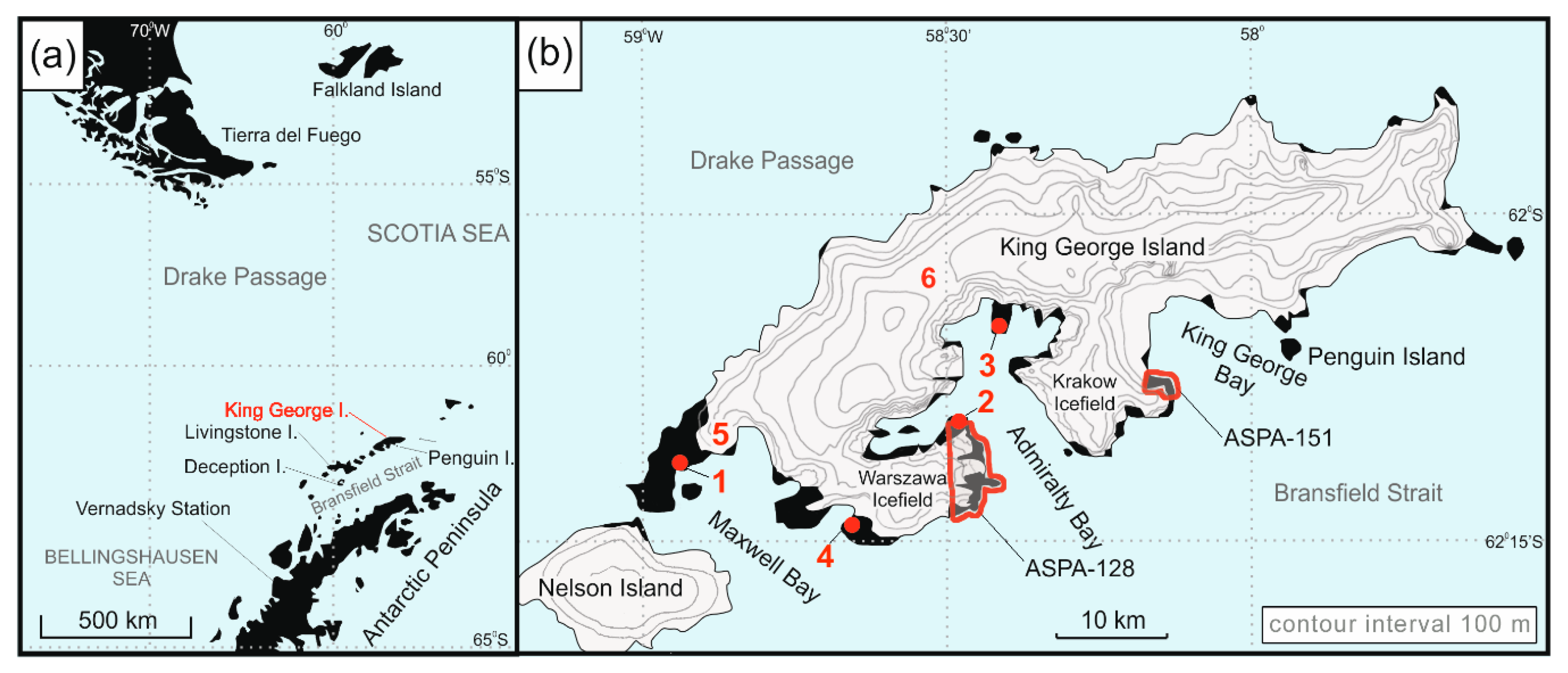
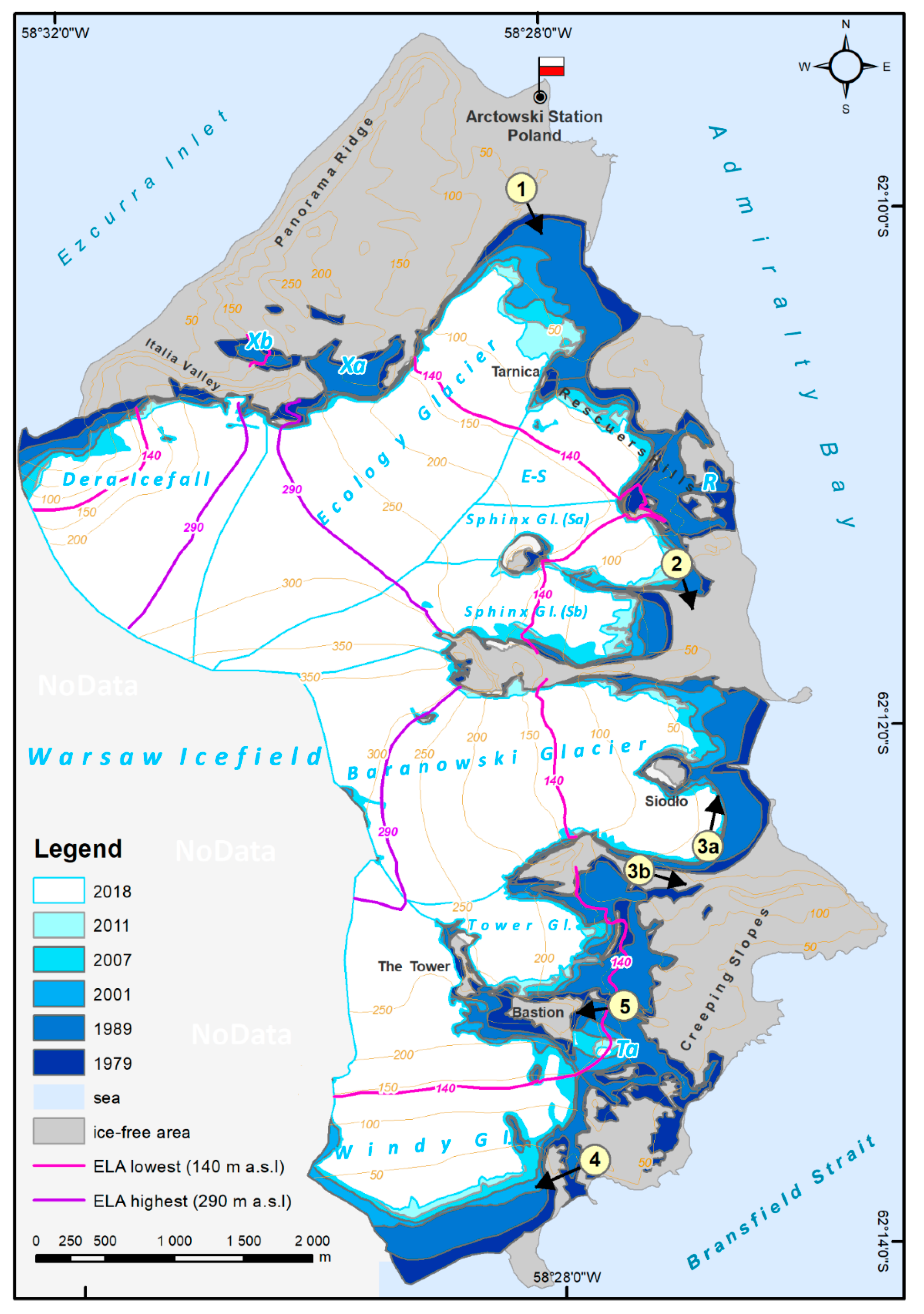
1.1. Characterization of the Research Area

The Antarctic Peninsula region and islands of the southern Atlantic Ocean have been identified as a region of notable dynamic change in glacial and climatic systems [1,2,3,4,5]. Over the last 50 years, large areas along the southern shoreline of King George Island have become ice-free. Several new nunataks have emerged, illustrating a significant reduction of glacier thickness. The late-Holocene maximum extent of glaciers on King George Island is marked by large ice-cored moraines, which were formed at the termination of the Little Ice Age (LIA) at the beginning of the 20th century [6]. Lichenometric studies of moraine ages in ASPA-128 and ASPA-151 (Antarctic Specially Protected Areas) indicate that the post-LIA glacier retreat was relatively slow until the 1940s [6]. The first field studies of glaciers in Admiralty Bay were conducted in the 1950s and reported a general reduction in ice extent [7]. Since the 1950s, an increased glacier retreat has been reported on King George Island by numerous studies [6,8,9,10,11,12]. An increase in surface temperature was also observed over the past several years. According to a simple ice dynamic model described by Knap et al. [13], such conditions are likely to affect the glacial state of the King George Island ice caps. Moreover, there is evidence of a glacier mass balance deficit and increases in surface energy exchange in this region [11,14,15]. Most of the previous studies of glaciers retreat in ASPA-128 simply documented changes in the front positions of glaciers in different years on maps. These studies were in different scales, mostly focused on Ecology Glacier, did not include spatial analysis, and did not account for the different behaviours exhibited by dissimilar glacier types. Therefore, it is difficult to compare these results to each other and to calculate glacier retreat rates.

For ASPA-128, there are no reports comparing fluctuations in glacier retreat with the climate data during the period of intensified reduction in glaciers extent between 1979–2018. Therefore, the aim of this study is to investigate the rate of the reduction in glaciated area for five periods—1979–1989, 1989–2001, 2001–2007, 2007–2011, and 2011–2018—for different types of glaciers.

Glacier retreat had a profound impact on local ecosystems including mammals, birds, and vegetation. The diverse avian and mammalian species and vegetation are the reason why the protected area of ASPA-128 was created. It has been shown that newly ice-free areas are dynamically colonised by plant communities [16] and nesting bird populations. Algae, lichens, mosses, fungi, and plants have colonized these recently formed ice-free areas on the glacier forefields and nunataks [17,18]. These include alien species of Poa annua L., which were first found by the author during the mapping of the forefield of the Ecology Glacier in February 2009 (reported by Olech and Chwedorzewska [19]). Additionally, new breeding areas became available for seals and birds. Therefore, it is important to document changes in glacier extent and also to identify the cause of these changes. To this point, there has been no integrated study of glacier retreat for ASPA-128 comparing how fast and how much of the area became ice-free between 1979 and 2018 as a result of climate change on King George Island (Figure 1).

1.2. Remote Sensing Data for King George Island

In the area covered by ASPA-128, it is difficult to conduct scientific research due to numerous obstacles, mainly cliffs and ice crevasses. The glacial systems are not extensive, the main glaciers flow from the Warszawa icefield toward the sea but, additionally, smaller glaciers are cut off from the supply from the icefield above. The features of this system make the glaciers very sensitive to climatic changes, but, because of their size, the ranges of ice must be determined precisely. This requires the use of an appropriate method of mapping and testing at the right time when the winter snow cover will already melt and when fresh snow will not yet cover the terrain in a way that prevents testing. The best period for fieldwork is February–April. However, it varies between years. For the above reasons, the most effective method for field research is the use of high-resolution aerial or satellite images. Based on the authors’ experience, in this work, the images with a spatial accuracy higher than 10 m were considered, however, less precise data were tested as well. The most important sources of remote sensing data taken into account in this work are discussed below.

• Satellite observation systems: Landsat is the pioneering remote sensing satellite program which has provided continuous multispectral data of the Earth’s land surfaces since 1972. With the launch of the L3 sensor in 1978, the possibility of acquiring images at a resolution of 30 m appeared. The next milestone was obtaining multispectral images from the TM (L4) sensor released in 1982. Since then, Landsat satellites have been recording the Earth’s surface with a revisit time of 16 days. In 1993, a sixth generation of satellites equipped with an ETM sensor was launched. This sensor enabled the acquisition of panchromatic photos at a resolution of 15 m, which greatly improved the possibilities of ice separation from the ground and the same detection of the range of small glaciers. Landsat 8 is the last observation LANDSAT satellite launched on 11 February 2013. It also has the ability to acquire panchromatic photos in 15 m resolution (OLI: Operational Land Imager sensor), but compared to the ETM sensor, the spectral resolution has been limited from 0.52–0.90 to 0.500–0.68 (µm), which means that the sensor is not sensitive to near infrared. This results in lower sensitivity to water detection, which in the case of research, is of great importance. For 2020, the next satellite is tentatively scheduled for launch by the NASA/USGS operator. Landsat-9 will be equipped with near-identical copies of the OLI and TIRS (Thermal Infrared Sensor) instruments that were flown on Landsat-8. Landsat databases are public, which is a very important fact for scientists, allowing their use in non-commercial and low-budget projects [20].
  • The second public land observation system that provides archived data with high spatial resolution is The Advanced Spaceborne Thermal Emission and Reflection Radiometer (ASTER). It provides satellite images since February 2000. The images consist of 14 channels, including 4 with a spectral resolution of 15 m (green/yellow; red; NIR1; NIR2). Archival data can be downloaded with a free registered account from either NASA’s Earth Data Search delivery system [21] or from the USGS Earth Explorer [22].
  • Copernicus is actually one of the most ambitious Earth observation programmes headed by the European Commission (EC) in partnership with the European Space Agency (ESA). One of the most important part of this programme is developing a new family of missions called Sentinels. Each one will provide accurate, timely, and easily accessible information to improve the management of the environment and understand and mitigate the effects of climate change. The first launched Copernicus satellite was Sentinel-1A, equipped with a C-band synthetic aperture radar (SAR). In 2015, the first Sentinel-2 satellite was launched and two years later, the second one, equipped with a similar sensor (MultiSpectral Instrument—MSI) designed for observing the Earth in 13 spectral bands, including 4 bands at a 10 m spatial resolution with a revisit time of 5 days. In the case of this program, the high spatial resolution of the data, short revisit time, and data availability makes this system crucial in conducting environmental studies, both on a global and regional scale [23].
  • The scientific community also has the possibility to take advantage of programmes offered by commercial suppliers. As an example, Planet Labs Inc. is accepting applications from students, researchers, technical staff, and faculty at accredited universities for a Basic Account in the Education and Research Program. In this program, researchers have the opportunity to obtain 10,000 km²/month data, free of charge [24]. The main advantage of this Planet data is its high resolution (<5 m) and very frequent revisit time, which results in an almost 100% probability of obtaining satisfying data in such a cloud-covered region like the Southern Shetlands.
• Aerial photography. The Falkland Islands and Dependencies Aerial Survey Expedition (FIDASE) was an aerial survey of the Falkland Islands and the Antarctic Peninsula, including the South Shetlands Islands, which took place in the 1955–1956 and 1956–1957 southern summers. The mission was held by the British Antarctic Survey as the United Kingdom Antarctic Mapping Centre. The photographic collection comprises of about 12,800 frames taken in high-resolution on 26,700 square kilometres of the ground track [25].
  • On the King George Island, there are a number of national polar stations (Figure 1). As a part of the research was conducted there, aerial photography missions were carried out in order to obtain remote sensing data. These images, mainly due to their resolution and timing, are one of the best remote sensing materials for analysing the dynamics of glaciers. However, in this case, the biggest problem is the range of the photographed area and the lack of cyclicality in repeating the survey. Examples include the following: (1) the Polish aerial photography of Admiralty Bay and King George Bay from 1979 [26]; (2) the Chilean aerial photography of Fildes Peninsula taken in 1983–1984 [27]; (3) the Polish UAV photogrammetry mission of Arctowski Station environment carried out in 2014/2015 [28].
• KGIS project. In 1998, the Working Group of Geodesy and Geographic Information (WG-GGI) of the Scientific Committee on Antarctic Research (SCAR) started an initiative for the implementation of GIS for the King George Island. This project, named KGIS, was the most comprehensive topographic database for this region. All available maps, aerial photography, satellite images, and geodetic surveys were compiled into the geographical information system. The reference data were the SPOT satellite mosaic based on SPOT-3, -4 XS images from 1994, 1995, and 2000 with a spatial resolution of 20 m. KGIS was also used in the research on the dynamics of glaciers [27].

The availability of public satellite data for the analysed area is summarised in

Table 1. The public archival satellite data available for ASPA-128, in the Australian summer months from 1978 to 2018, based on the USGS Earth Explorer: https://earthexplorer.usgs.gov/.

	01.02–30.04
	Landsat		Aster		Sentinel-2
	All	0–10% (Scene Cloud Cover)	All	0–10% (Scene Cloud Cover)	All	0–10% (Scene Cloud Cover)
1979–1981	6	0	x	x	x	x
1982–1984	0	0	x	x	x	x
1985–1987	2	0	x	x	x	x
1988–1990	0	0	x	x	x	x
1991–1993	0	0	x	x	x	x
1994–1996	0	0	x	x	x	x
1997–1999	0	0	x	x	x	x
2000–2002	17(L7)	0	2	0	x	x
2003–2005	26(L7)	1	5	0	x	x
2006–2008	8(L7)	1	6	0	x	x
2009–2011	12(L7)	0	13	0	x	x
2012–2014	11(L7) + 21(L8)	1 + 0	11	0	x	x
2015–2017	67(L8)	3	1	0	31	1
2018	22(L8)	1	x	x	16	1

x: data not available.

. Materials that were directly used for analysis are discussed in detail in the next chapter.

1.3. Climate Conditions on King George Island and Topo-Climate of ASPA-128

On King George Island, a temperature increase of 0.19 °C/10 years (r < 0.05) was observed during the period 1948–2011 [1]. This is one of the fastest temperature increases observed in the Southern Hemisphere. The change rate of the increase varied from year to year, with the largest warming observed for the winter months (0.36 °C/10 years). No temperature increase was noted during the spring months. The pace of the temperature and precipitation change from Bellingshausen Station varies over different periods (Figure 2). The precipitation on King George Island is characterized by substantial inter-annual variability (Figure 2). In the years 1968–2007, the annual sum of precipitation at Bellingshausen ranged from 434.2 mm to 893.7 mm. The mean values of precipitation decreased from 669 mm in 1968–1978 to an average of 545 mm for 2000–2006 (Figure 2). From 1968–2007, a decreasing trend in the total precipitation of 2–4 mm/year was observed.

The northern border of ASPA-128 is located 500 m south of Arctowski Station. The climatic conditions in ASPA-128 are influenced by large areas covered by glaciers and snow, as well as altitude and local atmospheric circulation, particularly katabatic and Foehn winds. The highest point of the Warszawa Icefield, which is a zone of accumulation for glaciers in ASPA-128, is nearly 450 m a.s.l. The climate characteristics from Arctowski Station (1977–1998, all data from Marsz and Styszyńska [29]), which is located at sea level, is described below. The mean annual air temperature for 1977–1998 was −1.6 °C and was characterized by a small seasonal amplitude. The average is similar to the Jubany and Ferraz stations and higher than at Bellingshausen Station due to the Foehn effect (Figure 2). Low-pressure centres moving around the Antarctic Peninsula result in highly variable weather with wind blowing predominately from the northern and western sectors. Due to such a minor decreasing trend, a significant portion of the air masses that reach Admiralty Bay cross over the island and are advectively warmed while falling from a 600–700 m a.s.l. elevation from the Arctowski Icefield summit to sea level. Precipitation varies significantly between the Bellingshausen and Arctowski stations due to the local topography and the Foehn effect. However, the annual sums of precipitation follow vaguely a similar trend between different stations on King George Island. The directly measured annual precipitation average at Arctowski Station is nearly 450 mm for the 1977–1998 period. The strong winds (4.5 m/s average for 1977–1998) also cause irregular accumulation and re-deposition of snow either on the island or off into the ocean, which results in the inaccurate measurement of snowfall totals.

The goal of this study is to examine the temporal variability and scale of glacier retreat in the eastern part of the Warszawa Icefield in the Antarctic Special Protected Area No. 128 (ASPA-128, Figure 1) on King George Island on the background of the observed changes in weather elements.

2. Materials and Methods

2.1. Detection Accuracy of the Marginal Zone of Glaciers—Landsat Case Study

In our research, the main criterion for selecting the remote sensing data for analysis was the ability to determine the ice border by identifying the sharp boundary between ice and land or the clear border between ice and the dead ice zone. The need to include in the image the entire studied region in a given year was also assumed. Fieldwork conducted by the authors (1999–2001, 2007) allowed for the collection of this type of data in the studied region and gain experience in interpreting aerial and satellite images. The preliminary analysis of the use of LANDSAT and ASTER images showed a limited possibility of obtaining this data, mainly due to cloudiness (Table 1). Additionally, not all the images with cloudiness below 10% met the quality requirements (no full coverage, clouds in the area of research).

The high resolution of the Planet and Sentinel images should not raise any doubts when detecting ice borders for such small glacial systems as found in the South Shetland Islands. However, in the case of Landsat data, one may be afraid that images recorded in individual bands with different resolutions are not detailed enough for the precise detection of the ice border. In order to answer this question and decide to include this data for further analysis, a preliminary test was carried out. It consisted of comparing the course of the ice border determined on the basis of the most detailed data Planet data with the map being a processed image of Landsat-8. Both types of data were obtained for a similar period (P: 2018/03/10; L: 2018/03/09).

The proposed methodology consists of the following steps:

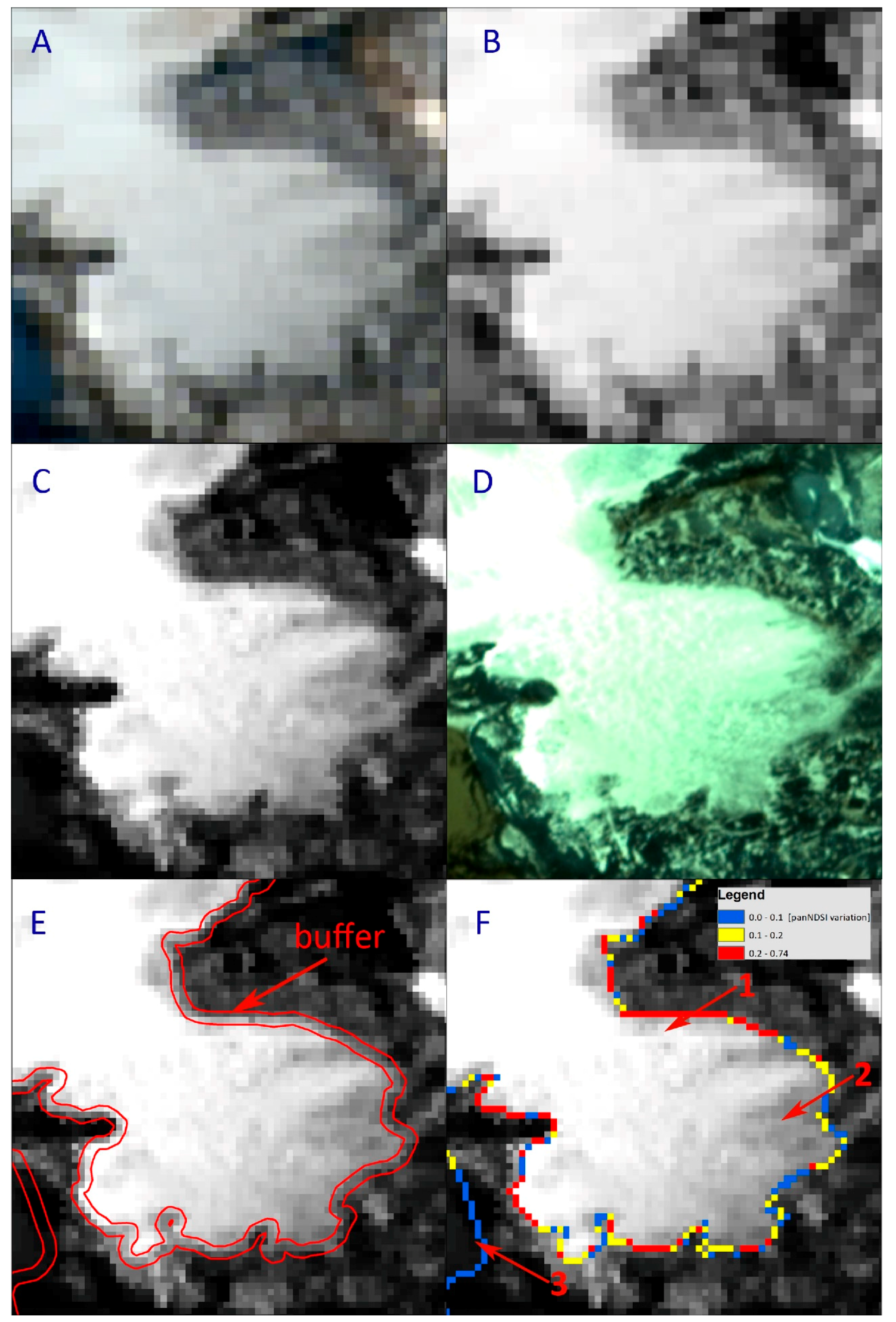
• NDSI index map. The image after geometric and radiometric correction completed in the ENVI software (© 2018 Harris Geospatial Solutions, Inc., Colorado, CO, USA) was classified to the map of Normalised Difference Snow Index (NDSI) using the following algorithm [31] (Figure 3A,B):

  $$\mathrm{NDSI}=\frac{\mathrm{Green}-\mathrm{SWIR}1}{\mathrm{Green}+\mathrm{SWIR}1}$$

  where Green: (0.52–0.60 µm) and SWIR1: (shortwave infrared) band (1.55–1.75 µm).
  The NDSI index is based on the spectral characteristics of ice and snow. In general, in the entire visible spectrum, the reflection is very high: about 90% for snow and 65% for ice of glaciers. In contrast, in the shortwave infrared spectral reflection can be even lower than 10% [32].
• panNDSI index map. A Panchromatic layer of Landsat (15 m resolution) was normalized to the range of 0–1 and multiplied by the NDSI index (pixel by pixel). As a result, a spatially and radiometrically enhanced NDSI map was generated in the resolution of 15 m. This layer was named the panNDSI index map (Figure 3C).
• Sensitivity analysis of the panNDSI index map to the detection of the glacier border. From the glacier border determined on the basis of the Planet image, a buffer zone was created at a distance equal to the panNDSI map resolution (2 × 15 m; see Figure 3D,E). All pixels of the panNDSI map located inside the buffer were clipped. For such selected pixels, local statistics were calculated in a moving window with a size of 2 × 2 pixels. Based on the knowledge of the spectral reflection characteristics of ice [32], it was assumed that a difference of less than 0.1 between the panNDSI index values will not allow for a detailed distinction of the ice-ground boundary (Figure 3F). As the local variation increases for pixels arranged along the ice border, the higher the possibility of automatic or semiautomatic classification.

Case study results. The above analysis shows that, based on the panNDSI map developed at a resolution of 15 m, there is a high probability of determining the ice border while maintaining the required accuracy in this area. As illustrated in Figure 3F, at 33.9% of the border length, the result was good, at 35.7%, it was very good. For 30.4% of the border length, there is a possibility of making a mistake bigger than assumed in this study in the glacial systems dynamics. Based on the study of the Tower glacier, it can be seen that the designated intervals accurately reflect the features of the image and the marginal zone of the glacier. In the zone of a sharp border ‘ice-moraine’, the highest accuracy was obtained (arrow 1); in the zone of ‘dirty ice-dead ice’, the accuracy clearly decreases (Figure 3F, arrow 2). There is also a strong impact of shadows on the detection capability of this method (Figure 3F, arrow3).

The presented methodology and results allow us to accept the possibility of using Landsat images in future research in this area.

2.2. Remote Sensing and Spatial Data

Based on the review of available databases (Section 1.2), the seven periods have been chosen for the study of the fluctuation of glacial retreat rates. Due to the limited availability of the data, it was not possible in each case to determine equal or approximate intervals.

Year 1956. Aerial photographs taken in 1956 by the Falkland Island and Dependencies Aerial Survey Expedition were the earliest available sources of spatial information for ASPA-128. These photos were scanned at a 600 DPI resolution and calibrated using ground control points (GCP) with a calibration accuracy of 0.5 m. Due to the presence of snow cover, only fragments of the Baranowski and Ecology glacier fronts were mapped (Figure 4).

Year 1979. In the subsequent years, a number of cartographic product extents were published. Aerial photographs taken during the summer of 1978/79 were used to create the detailed ‘Orthophotomap of ASPA-128 scale 1:10,000’, which illustrates the glacier positions during the Antarctic summer of 1978/1979 [26]. The map was made based on the selection of fifteen aerial photos taken on 6 February 1979 with an AFA/BAF camera (210 mm focal lens) and subsequently scanned at a 600 DPI resolution. The photos were rectified according to the ground control points, which were obtained by the GPS survey conducted in 2007. For the complete orthorectification process, the digital elevation model was used. The DEM was interpolated based on set elevation points gathered by GPS surveys in 2001 and 2007. After interpolation, the DEM was corrected to the elevation state in 1979 by the analysis-significant differences, which are visible by comparing the ice elevation in 1979 and 2007. As a result, the raster resolution is 0.3 m and the accuracy is 2 m.

Year 1989. The next map of ASPA-128 used in this study was the ‘Map of Admiralty Bay scale 1:50,000’ [33]. The map illustrates glacier fronts in 1989. Archival sketches and remarks on more detailed scales created by Battke using theodolite measurements were used to improve the overall accuracy. These materials allow for the recognition of glacier fronts with a 5–10 m accuracy.

Year 2001. In 2001, the first differential GPS surveys of the ASPA-128 recorded glacier front positions; the measurements were repeated in 2007 [26,34]. The field surveys (in 2001) were carried out using dual-frequency Ashtech Z-12 GPS receivers. Direct mapping included two stages: a dynamic mapping of glacier fronts and static measurements for the GCP points that were used for the ortho-rectification of archival aerial photographs.

Year 2007. In 2007, DGPS measurements were carried out using MLR SP 24XC GPS receivers. The determination of glacier margins from the 2001 and 2007 field-based GPS surveys had an instrument accuracy of 1–2 m and an accuracy of field measurements of 1–2 m. Track logs along the glacier terminus were recorded at the end of the austral summer when no snow cover was present.

Year 2011. Glacier front positions in 2011 were mapped on Google Earth⁽™⁾ (GeoEye-1, DigitalGlobe⁽™⁾ satellite image from 2 February 2011), which were rectified and calibrated to our previous maps using the DGPS points. The accuracy of the glacier extents in 2011 was 2 m.

Year 2018. The most current satellite data used in this work comes from 2018. Two PlanetScope⁽™⁾ images were obtained with a ground resolution of 3 m. The first picture with very good quality (visible sharp separation between snow-covered glacier-ice and ground) comes from 13 February. The second one was taken on 10 March. In comparison with the previous Planet scene, the glacier-ice is already visible after the winter snow has melted. However, fresh snow is also present, mainly in the hollows of the ground.

Integration of the archival data. All the acquired remote sensing data have been processed by geometric and radiometric correction and completed in the ENVI software. The Universal Transverse Mercator (UTM 21S) was chosen as a common reference system, while all the images were checked and calibrated to the orthophotomap from 1979, which was prepared on the basis of aerial photographs with the highest resolution, and the orthorectification process was carried out on the basis of terrain points where the geographical coordinates were determined using the DGPS method [26,34]. The pre-processed images (1956, 1979, 1989, 2001, and 2018) were entered into the ArcGIS project (© ESRI, Inc., Redlands, CA, USA). The geobase was completed with vector data (SHP) representing previously determined ranges of glaciers (2001, 2007). Direct mapping using GPS permitted the precise identification of glacier margins, dead-ice zones, and perennial snow covers. Due to the high quality of the aerial photographs and satellite images (Geo-Eye1 and PlanetScope), the determination of glacier boundaries did not require advanced image analysis techniques and was carried out by the vectorization of appropriately sharpened images (histogram analysis and stretching). All images (excluding 1956 data) were gathered when the snow cover was absent (or insignificant), facilitating the high-resolution tracking of numerous features, including large-glacier fronts, small-glacier margins, and permanent snow/ice patches. The most problematic cartographic data adapted to determine the course of the glacier border (cause of the scale, 1:50,000) was the map from 1989 [33]. In order to improve spatial accuracy, archival sketches were used. This task was carried out in parallel to the first kinetic GPS survey conducted in 1999 during the 23rd polar expedition to the Arctowski Station, where one of the co-authors of the presented study had an opportunity to personally consult on the data quality with Mr Battke, the map’s author. The collected preliminary results served as a basis for the GIS project developed for ASPA-128 since that time and, finally, were used in this study.

In the next step, the glacier ranges from all the analysed periods, coded as shapefiles, were converted to polygons, which allowed for the study of the diminishing glacier area for both types of glaciers (land-terminating and tidewater). The base map for the detailed analyses of individual glaciers is presented in Figure 5. In comparison, previous publications on the determination of glacial change in the Admiralty Bay using satellite imagery [8,35] focused mainly on determining the retreat stages of tidewater glaciers. Some of these satellite images were taken at times when snow cover was still present and, consequently, the interpretation of glacier borders terminating on land was very difficult.

The areal extent of each glacier was determined for 1979, 1989, 2001, 2007, 2011, and 2018 (Figure 5). The glacier extents based on aerial/satellite photos and maps were digitized manually with the accuracy limited by the resolution of materials. Areas of dead ice covered by moraines were not included in the estimate of the glaciated area for any of the analysed periods. Estimates of area change within each zone and period are based on a spatial analysis. Since the number of observational records available is not comparable with the record of local climatic change, the mean ratio of retreat (km²/year) was calculated for each period in 50-m altitude intervals for each glacier (

Table A1. The change in the glaciated area and ratio of the glaciated area loss for 1979–1989, 1989–2001, 2001–2007, and 2007–2011 for land-terminating glaciers (L) and tidewater glacier (T) in ASPA-128. The sums and averages for each altitude interval, and the sums and averages for each of the analyzed periods are in bold.

Area (km2)	Altitude (m a.s.l.)
	0–50	50–100	100–150	150–200	200–250	250–300	300–350	350–400	Total Area SUM (km2)
L 1979	0.348	1.159	1.347	1.107	0.829	0.244	0.303	0.200	5.538
L 1989	0.160	0.929	1.163	1.006	0.775	0.228	0.300	0.200	4.762
L 2001	0.037	0.556	0.789	0.816	0.689	0.213	0.298	0.200	3.598
L 2007	0.030	0.486	0.716	0.744	0.674	0.205	0.297	0.200	3.352
L 2011	0.014	0.353	0.650	0.655	0.659	0.197	0.295	0.200	3.022
L 2018	0.000	0.259	0.619	0.630	0.642	0.196	0.295	0.200	2.842
T 1979	2.472	1.928	1.590	1.578	1.766	3.765	0.988	0.137	14.224
T 1989	2.024	1.855	1.563	1.554	1.709	3.679	0.969	0.136	13.490
T 2001	1.058	1.711	1.529	1.536	1.649	3.625	0.962	0.137	12.209
T 2007	0.720	1.575	1.509	1.509	1.596	3.603	0.955	0.136	11.604
T 2011	0.518	1.413	1.444	1.463	1.561	3.570	0.939	0.137	11.046
T 2018	0.414	1.309	1.438	1.445	1.561	3.562	0.939	0.137	10.806
DELTA Area (−km2)	Altitude (m a.s.l.)
	0–50	50–100	100–150	150–200	200–250	250–300	300–350	350–400	Deglaciation SUM (km2)
L 1979–1989	−0.188	−0.230	−0.184	−0.101	−0.054	−0.016	−0.003	0.000	−0.776
L 1989–2001	−0.124	−0.373	−0.375	−0.190	−0.087	−0.015	−0.002	0.000	−1.164
L 2001–2007	−0.006	−0.070	−0.072	−0.072	−0.015	−0.008	−0.001	0.000	−0.245
L 2007–2011	−0.017	−0.133	−0.066	−0.089	−0.015	−0.008	−0.002	0.000	−0.330
L 2011–2018	−0.014	−0.094	−0.031	−0.025	−0.017	−0.001	0.000	0.000	−0.181
L 1979–2018	−0.348	−0.900	−0.727	−0.478	−0.187	−0.048	−0.008	0.000	−2.697
T 1979–1989	−0.448	−0.073	−0.027	−0.024	−0.057	−0.086	−0.019	0.000	−0.734
T 1989–2001	−0.965	−0.144	−0.034	−0.018	−0.060	−0.054	−0.006	0.000	−1.281
T 2001–2007	−0.338	−0.136	−0.020	−0.027	−0.053	−0.022	−0.008	0.000	−0.604
T 2007–2011	−0.202	−0.162	−0.065	−0.046	−0.035	−0.033	−0.015	0.000	−0.559
T 2011–2018	−0.104	−0.104	−0.006	−0.018	0.000	0.008	0.000	0.000	−0.239
T 1979–2018	−2.057	−0.619	−0.152	−0.133	−0.205	−0.203	−0.048	0.000	−3.417
RATIO (km2/year)	Altitude (m a.s.l.)
	0–50	50–100	100–150	150–200	200–250	250–300	300–350	350–400	Retreat (km2/year)
L 1979–1989	−0.019	−0.023	−0.018	−0.010	−0.005	−0.002	0.000	0.000	−0.078
L 1989–2001	−0.010	−0.031	−0.031	−0.016	−0.007	−0.001	0.000	0.000	−0.097
L 2001–2007	−0.001	−0.012	−0.012	−0.012	−0.002	−0.001	0.000	0.000	−0.041
L 2007–2011	−0.004	−0.033	−0.017	−0.022	−0.004	−0.002	0.000	0.000	−0.083
L 2011–2018	−0.002	−0.013	−0.004	−0.004	−0.002	0.000	0.000	0.000	−0.026
L 1979–2018	−0.009	−0.023	−0.019	−0.012	−0.005	−0.001	0.000	0.000	−0.069
T 1979–1989	−0.045	−0.007	−0.003	−0.002	−0.006	−0.009	−0.002	0.000	−0.073
T 1989–2001	−0.080	−0.012	−0.003	−0.001	−0.005	−0.004	−0.001	0.000	−0.107
T 2001–2007	−0.056	−0.023	−0.003	−0.004	−0.009	−0.004	−0.001	0.000	−0.101
T 2007–2011	−0.051	−0.040	−0.016	−0.011	−0.009	−0.008	−0.004	0.000	−0.140
T 2011–2018	−0.015	−0.015	−0.001	−0.003	0.000	−0.001	0.000	0.000	−0.034
T 1979–2018	−0.053	−0.016	−0.004	−0.003	−0.005	−0.005	−0.001	0.000	−0.088

). The basis for the elevation was the DEM based on the 2007 survey. The DEM was corrected to the ice elevation state from 1979.

In order to assess long-term trends in the fluctuation of glacier front positions within ASPA-128, our results were compared with changes in the Equilibrium-Line Altitude (ELA,

Table 2. The changes in the Equilibrium-Line Altitude (ELA) heights on King George Island.

Glacier Mass Balance Year	ELA (m a.s.l.)	Reference
1969/1970	140	Orheim and Govoruhka 1982 [36]
1970/1971	170	Orheim and Govoruhka 1982 [36]
1985/1986	150	Jiawen et al., 1995 [37]
1991/1992	160	Braun and Rau 2000 [38]
1992/1993	200	Braun and Rau 2000 [38]
1993/1994	200	Braun and Rau 2000 [38]
1995/1996	200	Braun and Rau 2000 [38]
1996/1997	250–270	Braun and Rau 2000 [38]
1997/1998	180–200	Braun and Rau 2000 [38]
1998/1999	200–220	Braun and Rau 2000 [38]
2006/2007	290	this study
2012/2013	156	Sobota et al., 2015 [9]

), climate records (temperature and precipitation), and changes in the Positive Degree-Day sum (PDD) from the Bellingshausen, Jubany, and Ferraz stations on King George Island (Figure 1 and Figure 2). In addition, we used archival photographs and maps to analyse the reduction in glacier surface elevation. Such data were available for the Baranowski and Ecology glaciers at elevations below 100 m a.s.l. (for example, Figure 4 and Figure 5). The geomorphological mapping of glacier forefields that have become recently ice-free in ASPA-128 point toward landforms related to the surface melting of ice. Our initial field observations from ASPA-128 indicated slow glacier flow velocities.

The glaciers were divided into individual drainage areas based on the analysis of the course of contours. Additional adjustments were possible from aerial photos from 1979 and 2011 based on crevasses distribution and orientation (Figure 5). Next, the glaciers were identified as either tidewater or land-terminating. This approach allowed us to take into consideration the unique behaviour of each glacier type and to illustrate individual glacier profiles (Figure 6 and Figure 7). In the case of the graph shown on Figure 7, the area covered by glaciers was summed from the lower elevations upwards in 50-m altitude intervals. Only the selected Equilibrium-Line Altitude (ELA) heights are shown on this figure. The full list of the ELAs is presented in Table 2. Note that the study area extent did not allow for the measurement of the entire feeding area of some glaciers (for example, the Dera Icefall and Windy Glaciers). The tidewater glaciers in this study (Dera Icefall, Ecology, Baranowski and Windy glaciers) are typically large and are supplied directly from the Warszawa Icefield (300–400 m a.s.l.; Figure 5 and Figure A1). Parts of these glacier fronts terminate directly in Bransfield Strait, Admiralty Bay, or in shallow lagoons that are disconnected from the ocean during low tide. In 2011, these glaciers terminating in lagoons formed 10–30 m high ice cliffs that were unstable under tidal influences and, thus, experienced enhanced calving during austral summer. The land-terminating glaciers in this study (Thawing, The Tower, Sphinx, and small glaciers) branching from the Ecology Glacier (Xa, and Xb zone, Figure 5) are smaller and have zones of accumulation at lower elevations (200–350 m a.s.l.). Changes for each glacier zone were analysed in 50-m altitude intervals.

2.3. Climate Data

The changes in the climate record on King George Island were analysed and related to retreat observations. The longest record of both temperature and precipitation used in this study came from Bellingshausen Station (1968–2014, Figure 2). These data were compared with the same measurements from Arctowski Station (1977–1999, Figure 2), which is located close to the northern border of ASPA-128; Ferraz Station (1986–2013, Figure 2), located on the eastern side of Admiralty Bay (Figure 1); and Jubany Station (1986–2014, Figure 2), located on the eastern side of Warszawa Icefield (Figure 1).

Because it is important to assess the portion of temperature change capable of affecting the glacier melt, the mean daily temperature for all the days in which the temperature was above 0 °C was summed to calculate the annual sum of Positive Degree-Days (PDD) [39] for Arctowski Station in 2006 (data from other years were not available). The PDD were also calculated for Bellingshausen Station (1968–2010; Figure 2). The archival PDD data from Barrand et al. [30], from Ferraz (1987–2010), and from Jubany (1991–2009) stations were also used. The equilibrium line altitude (ELA) was also calculated for 2006 using data from glacier monitoring (including bi-weekly stationary field photographs of glaciers in ASPA-128 from seven different locations).

3. Results

A full analysis of the glaciers area, the changes between the studied periods, and the average annual rate of glaciers retreat are presented in Table A1 (see Appendix A). The most significant result for this study—the dynamics of glaciers—is shown in Figure 6 as a cumulative chart (for each altitude intervals, separately for each period). Additionally, against the background of the dynamics of glaciers, the temperature, precipitation, and PDD lines were applied. The Bellingshausen meteorological data were used as the longest available measuring series (Figure 2 and Figure 6).

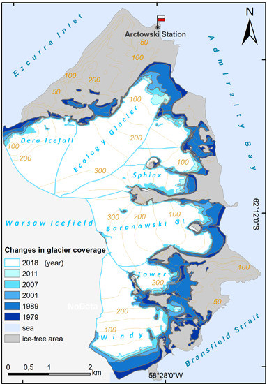
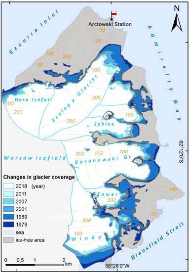
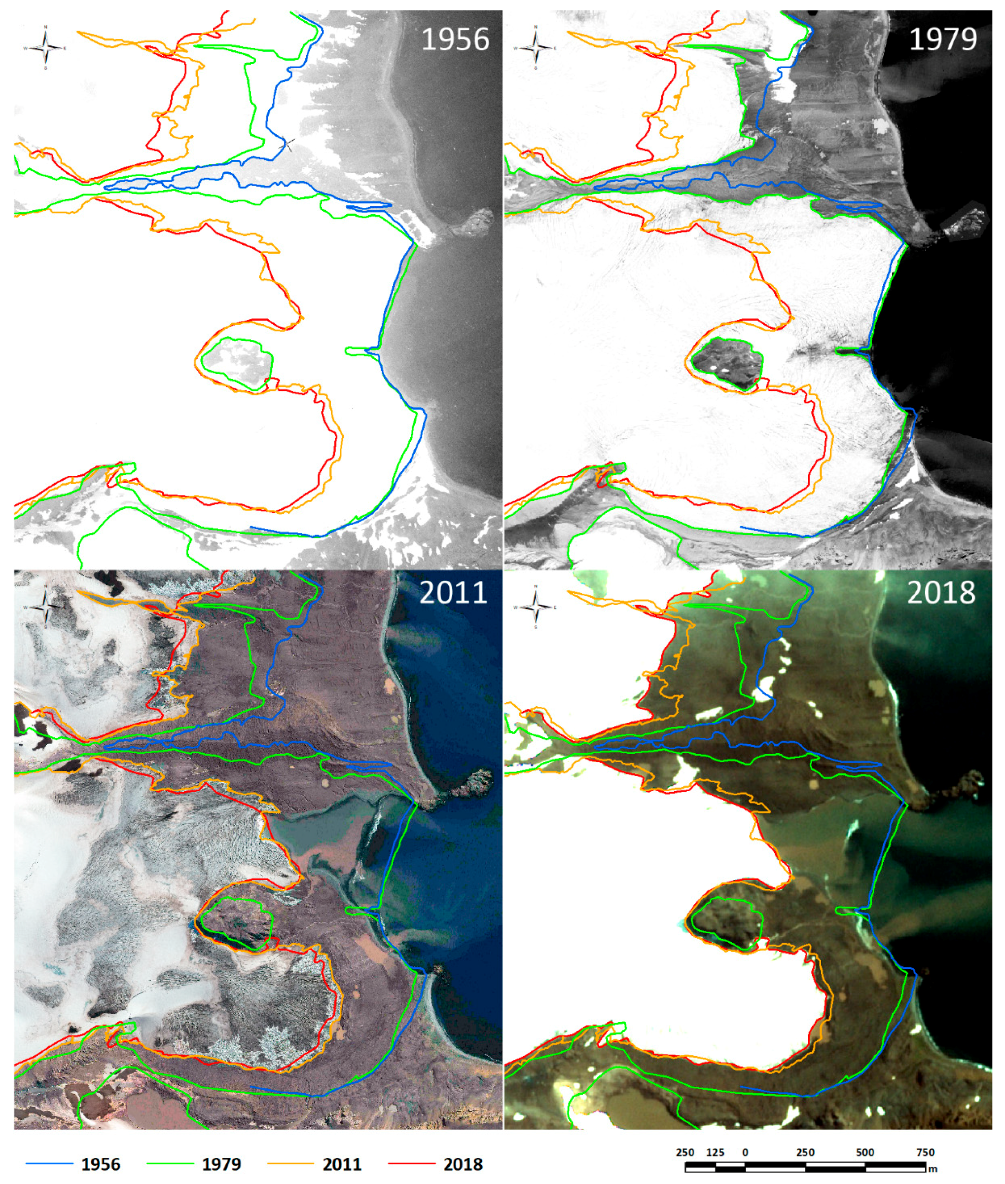
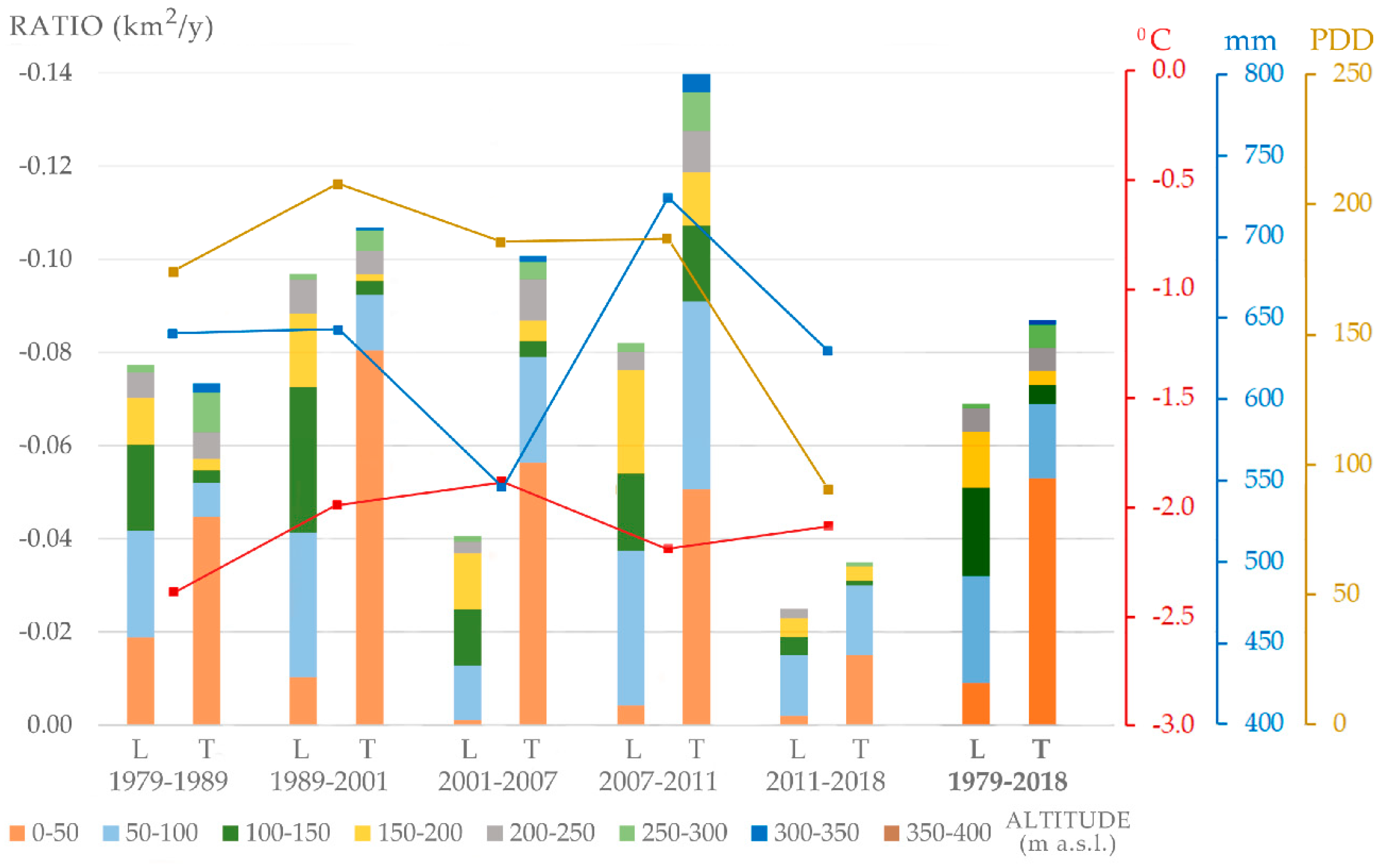
3.1. Glacier Retreat in ASPA-128 (1979–2018)

3.1.1. Period 1 (1979–1989)

The retreat of all the glacier fronts was observed in ASPA-128 in the early 1980s (Figure 4 and Figure 5). The most visible changes are related to small glaciers and glaciated areas located at lower altitudes with limited connection to feeding areas (Creeping Slopes, Rescuers Hills). Between 1979 and 1989, the glaciated area in ASPA-128 was reduced by 1.51 km². The area loss of land-terminating water glaciers was greater at 0.78 km² than that of tidewater glaciers at 0.73 km² (average of −0.08 km²/year for land-terminating glaciers and −0.07 km²/year for tidewater glaciers). In this period, the retreat of tidewater glaciers was the fastest (−0.045 km²/year) for the first analysed altitude interval (0–50 m a.s.l.). It was more than twice as fast in comparison to the same level of land-terminating glaciers (Figure 6). The total glacier area loss was equivalent to 7.6% of the original glaciated area in 1979.

3.1.2. Period 2 (1989–2001)

Between 1989 and 2001, the glaciated area reduced by 2.45 km² (−1.16 km² for land-terminating glaciers and −1.28 km² for tidewater glaciers) and the average rate of annual recession was higher in comparison to the previous (1979–1989) and subsequent (2001–2007) periods (average of −0.1 km²/year for land-terminating glaciers and −0.11 km²/year for tidewater glaciers). In this period, land-terminating glaciers retreated nearly completely from the 0–50 m a.s.l. elevation. Additionally, in this interval, the fastest (−0.8 km²/year) retreat among all the periods and intervals was observed for tidewater glaciers (Figure 6, Table A1). The total glacier loss is equivalent to 13.4% of the glaciated area in 1989, bringing the reduction in the glaciated area since 1979 up to 20%.

3.1.3. Period 3 (2001–2007)

After 2001, the pace of the glaciers’ retreat returned to pre-1989 levels. In comparison to the 1989–2001 period, the average annual ratio of glacier retreat decreased in each zone (Figure 6). The largest area loss was observed for the Ecology and Baranowski glaciers, which are tidewater glaciers. During the period 2001–2007, an exceptionally large area loss of the Thawing Glacier was observed (73% loss of the 2001 area). Between 2001 and 2007, the glaciated area in ASPA-128 was reduced by 0.85 km² (0.25 km² land-terminating and 0.6 km² tidewater glaciers) with an average of −0.04 km²/year for land-terminating glaciers and −0.1 km²/year for tidewater glaciers. A part of the diminishing rate of the land-terminating glaciers’ retreat between 2001–2007 can be explained by the retreat of this type of glacier from areas below 50 m a.s.l. prior to 2001. These areas contributed to the greatest loss of area in previous years. Nevertheless, the upper regions of land-terminating glaciers (for example, areas 50–150 m a.s.l., Table A1) between 2001–2007 have retreat ratios that are about four times lower than the same areas in the 1989–2001 period.

3.1.4. Period 4 (2007–2011)

Between 2007 and 2011, the glaciated area in ASPA-128 was reduced by 1.35 km² (−0.43 km² land-terminating and −0.93 km² tidewater glaciers). The pace of the glacier retreat increased to an average of −0.08 km²/year for land-terminating glaciers and −0.14 km²/year for tidewater glaciers. These values are comparable to the 1989–2001 period ratios.

In total, from 1979 to 2011, 5.7 km² of ice-covered areas became ice-free, which is 27.4% of the glaciated area in 1979 (Figure A2, Figure A3 and Figure A4). As a result of the glacier retreat between 1979–2011, some small glaciers disappeared almost completely (for example, the Thawing Glacier) and most of the nunataks at lower elevations (for example, Tarnica, Siodło, The Tower, Bastion) are now connected to ice-free areas (Figure A5). Additionally, a few new nunataks have appeared. The analysis of archival materials showing the altitude of the glacier edges on nunataks allowed for an estimation of the decrease in ice surface height. Two nunataks were studied: the Siodło (Baranowski Glacier) and Tarnica (Ecology Glacier) nunataks. Since 1979, the reduction in the ice level estimated from those nunataks was 15–20 m (0.5–0.7 m/year on average, Figure A5).

3.1.5. Period 5 (2011–2018)

During the last 7 years, the lowest rate of regression was recorded in the entire analysed period (1979–2018). A clear retreat of glaciers (ca. 0.013–0.015 km²/year) is observed only at an interval of 50–100 m a.s.l. for land-terminating glaciers and at intervals of 0–50 and 50–100 m a.s.l. for tidewater glaciers. The ratio for the other intervals is close to the measurement error (Figure 6). In this period, it can also be noticed that the Windy glacier changed its status from tidewater to land-terminating (Figure A1). The expansion of the ice-free area from around the nunataks and the decline in the ice surface height is still observed, but the pace of these changes is significantly lower than in the previous periods.

4. Discussion

The surface temperature warming observed in the Antarctic Peninsula region in the last few decades [2,3] resulted in a reduced seasonal snow cover [40], an increased ablation of glacier ice located below the glacier’s ELA [30], an increased snowfall which could increase the future ice discharge from feeding areas [41], and it may have caused an increased rate of sublimation and evaporation, further contributing to the removal of ~9% of precipitation in the Antarctic Peninsula region [42]. The summer temperatures on King George Island are above zero between December and February, and close to melting temperatures in spring and autumn, so, even a small degree of warming may have a significant impact on glaciers. Bintanja [14] calculated that, for the Ecology Glacier, an increase of the air temperature by 1 °C would intensify ablation by 15%. As a consequence of warmer temperatures, the melting season is longer and the accumulation of seasonal snow cover is reduced. Moreover, the temperature gradient between a glacier and its forefield is higher when snow cover is absent. The gradient can cause a positive feedback, which may, in addition, increase the surface melting at the front margin of a glacier. Since the number of days with snow cover decreases due to higher temperatures and smaller precipitation, it may also negatively affect the ice balance at the glacier front zone. Therefore, the temperature warming in spring and autumn is particularly important as it extends the ablation season, further diminishing the balance of glaciers. In the winter, melting occurs only during mid-winter thawing events [43,44]. These events are caused by dynamic weather systems bringing warmer air masses to the South Shetland region. The alteration of this circulation pattern may play an important role in increasing the frequency and severity of mid-winter thawing events.

The air temperature and precipitation trends for the period of 1968–2011 from Bellingshausen Station do not explain why the fastest ratios of glacier area loss occurred between 1989–2001. Between 1968–2007, the air temperature was increasing (at +0.2 °C/10 year) and the precipitation was decreasing (at −2.38 mm/year). Our results suggest that the rate of reduction in glaciated areas was the fastest between 1989–2001, compared with the 1979–1989 and 2001–2007 periods being twice as slow. Similar trends could be observed in annual PDD sums. The averages of PDD for the investigated periods from the Bellingshausen, Jubany, and Ferraz stations (Figure 2) indicate higher PDD values for the 1989–2001 period compared to 2001–2007. Additionally, the 1979–1989 averages from Bellingshausen Station are lower than the 1989–2001 average. The warmer period between 1989–2001 also stands out as the only period that had a faster ratio of glaciated area loss for land-terminating glaciers than tidewater glaciers (Figure 6), which suggests the presence of an elongated melt season during that period. This could explain the changes observed in the retreat ratios of land-terminating glaciers with ablation dominated by surface melting, as they would most quickly respond to the climate change between 1989–2001.

Rückamp et al. [8] showed very slow glacier flow velocities for the Bellingshausen Dome and Rückamp et al. [45] showed that the velocities on the Arctowski Icefield since 1997 were similar. Similarly, a study by Osmanoglu et al. [46] demonstrated slow surface velocities and a thickness in the lower elevations of the Warszawa Icefield system. Slow surface velocities and increasing PDD results in changes in the glaciers’ Equilibrium-Line Altitude (ELA). Between 1967 and 1999, the ELA on King George Island rose from approximately 140 m a.s.l. [27] to 220 m a.s.l. (Table 2). In 2006, the highest level of ELA was observed (290 m a.s.l.), but it is worth notice that 2006 is the warmest year in the period 2001–2007 (Figure 2) and the ELA of the early 2000s may have been lower. Increased surface melting in ASPA-128 and the resulting ELA shift towards higher elevations may explain the almost complete disappearance of small cirque glaciers, such as the Thawing Glacier, with a feeding area between 120–200 m a.s.l. Similar observations of the almost complete degradation of small cirque glaciers located below 250 m a.s.l. were reported on the Keller Peninsula near Ferraz Station in Admiralty Bay [11]. Larger land-terminating glaciers in ASPA-128 (for example, Sphinx and Tower glaciers) with feeding areas below 300 m a.s.l., also experienced significant area loss (Figure 6). Correspondingly large decreases in the ice cover were observed 30 km to the east in ASPA-151 (for example, Reference [6] for glaciers fed from the Krakow Icefield (300 m a.s.l.)). As simulated by Rückamp et al. [8], the small independent ice cap on Bellingshausen Dome (summit at 270 m a.s.l., eastern King George Island) will disappear within the next 300 years under the current climate conditions.

The overall results confirm the amplified recession of glaciers on King George Island observed since the 1970s. From 1956 to 1979, the recession of the Ecology Glacier ice cliffs was observed. However, the available data were insufficient to calculate the glaciers’ retreat rates. During the 1989–2001 period, the glaciers’ retreat rates increased (to −0.1 km²/year for land-terminating glaciers and −0.11 km²/year for tidewater glaciers) in comparison to the first studied period, causing some nunataks to become connected with glacier forefields in ASPA-128. A decrease in the rainfall and a cyclical occurrence of ‘warm’ years (average annual temperature above −1 °C) were frequently observed (Figure 2) as a result of the ELA being lower (Table 2). During the third studied interval (2001–2007), glacier retreat was similar for tidewater glaciers (−0.1 km²/year) and much slower for land-terminating glaciers (−0.4 km²/year) compared to those observed from 1979–1989. In the period of 2007–2011, the retreat ratios accelerated to −0.14 km²/year for tidewater glaciers and to −0.8 km²/year for land-terminating glaciers, and then unexpectedly dropped in the last period (2011–2018). Analysing the availability of the data in the conducted research, a clear lack of archival remote sensing materials can be seen for the period after 1979 to 2011 (Table 1). This deficiency was without any detriment to the results of the analyses complemented by field studies carried out in 2001 and 2007. However, high-resolution and high-quality remote sensing materials, available in 1985–1995, would significantly improve the interpretation of the results for this period. This applies mainly to period 2 (1989–2001), in which a sudden increase in the rate of deglaciation of tidewater glaciers and the rapid deglaciation of the area located in the interval of 50–150 m above sea level has been observed for land-terminating glaciers. Unfortunately, public remote data are not available for this period. However, in the period 2001–2018, the rate of deglaciation was analysed in detail, both due to the availability of remote sensing materials, as well as terrestrial measurements.

Glaciers of ASPA-128 terminate both on land or in shallow lagoons connected to either Bransfield Strait or Admiralty Bay. Land-terminating glaciers are influenced mostly by atmospheric processes (and, therefore, climate change), whereas tidewater glaciers experience complex and dynamic reactions to both oceanic and atmospheric systems, including ice calving [47]. Therefore, we analysed land-terminating and tidewater glaciers separately. The area loss of land-terminating glacier tongues can mostly be attributed to surface melting. For tidewater glaciers, ablation is dominated by the calving of glaciers, which allows for the faster reduction of glacier mass in comparison with surface ablation [47]. Pritchard and Vaughan [48] demonstrated widespread acceleration of tidewater glaciers in the Antarctic Peninsula region. The observations of Rückamp et al. [45] confirmed the different dynamics of land-terminating glaciers on the Potter Peninsula and tidewater glaciers terminating in Potter Cove (near Jubany Station). In our study, the difference between the overall retreat rate of land-terminating and tidewater glaciers for the 1979–2011 period was −0.099 km²/year for tidewater glaciers and −0.083 km²/year for land-terminating glaciers. The 1979–2011 average glacier retreat rates at various elevations indicated significant difference between these two types of glaciers. The land-terminating glacier retreat rates greater than −0.01 km²/year were observed up to 200 m a.s.l. with the fastest retreat (over −0.022 km²/year) between 50–150 m a.s.l., where the recent terminus of the glacier fronts is located. The tidewater glacier retreat ratios of −0.01 km²/year were observed between 50–100 m a.s.l. with the most dominant changes occurring between 0–50 m a.s.l. where the glaciers’ retreat rate was −0.061 km²/year (Table A1). In the last period, the retreat of glaciers has dropped unexpectedly and is observed only at an interval of 50–100 m a.s.l. for land-terminating glaciers and at an interval of 0–50 and 50–100 m a.s.l. for tidewater glaciers (Figure 6). There may be many reasons for this to happen. For example, reducing the mass of ice to a critical value (in case of land-terminating glaciers). Among the weather indicators, only PPD sums explain this sudden change in the dynamics of glaciers. The overall reduction in the length of the tidewater glacier fronts between 1979 and 2018 indicate the reduced ability for calving to occur (Figure 5). Compared to 1979, in the subsequent analysed periods, the length of the fronts of Ecology, Baranowski, and Windy glacier systematically decreased: (1989: 71%; 2001: 67%; 2007: 66%; 2011: 51%; 2018: 48%). This is particularly evident in the case of the Windy glacier, which has finally lost contact with the shore (Figure A1).

Our results provide detailed background information for a period when the glaciers’ retreat had a crucial impact on the maritime and land ecosystems in ASPA-128 and on King George Island. For example, between 1979 and 2007, several new hydrological features formed in terrain depressions, including lakes and lagoons. At higher elevations, a few new nunataks appeared and some areas previously separated by glaciers became connected. Periglacial and denudation processes began to modify the landscape, further increasing glacier ablation. The intensified surface melting provided increased freshwater discharge from glacial rivers and delivered more suspended material to the near shore environment of King George Island, all of which affected the local ecosystems [49,50]. Our study results demonstrated that new ice-free areas were added at different rates during different periods, which must be taken into account when studying the influence of environmental changes on the maritime and land ecosystems. It will be important to continue to monitor this process and its impact on the ecosystem as glaciers retreat. In recent years, new satellite sensors have extended this possibility. This mainly applies to satellite missions like Sentinel (ESA Copernicus Programme), Pleiades (CNES), and the satellite constellation of DigitalGlobe⁽™⁾ and Planet Labs⁽™⁾ which provide high-resolution images at short intervals of time. Based on the new remote sensing data, the deglaciation of the studied area is still observed and analysed but is not as rapid and obvious like in the period (1989–2007). An example of this is the comparison of a fragment of the Planet satellite image from 5 February 2018 [24] with remote data used for analyses (Figure 4). Another challenge for analysing the dynamics of glaciers will be the use of SAR images. In this case, Sentinel-1 gives possibilities for the analysis of this type of image in high spatial and temporal resolution. In comparison to visible images, SAR sensors have the ability to record data during cloud cover. This is extremely important in the West Antarctic region. The effect of cloudiness on the availability of classic satellite images is shown in Table 1. On the basis of the data presented in Table 1, it can be concluded that in the case of Landsat, only 3.6% (7 from 192) of images recorded cloud cover below 10%; in the case of the Aster satellite none of the archival images met this minimum criterion; and in the case of Sentinel-2 images, only 2 archival images from 47 (4.3%) met this condition. It should also be remembered that browser systems classify cloudiness automatically and not all listed images meet the quality criteria for this type of interpretation.

Based on the trend in satellite observation systems development, we can anticipate a widespread availability of high-resolution (spatial, spectral, and temporal) data for polar regions in upcoming years. Even now, the data can be calibrated and verified using UAVs’ low-altitude remote sensing, which is becoming less expensive year by year, with increasing technical capacity. Considering the above, scientists at polar research stations should already engage in the systematic monitoring of the glaciers’ dynamics using remote sensing. The following research studies can serve as examples: References [51,52,53,54]. Such activity, conducted for small glacial systems in the Antarctic, will certainly be a valuable contribution to the monitoring of the global effects of climate warming.

5. Conclusions

(1)

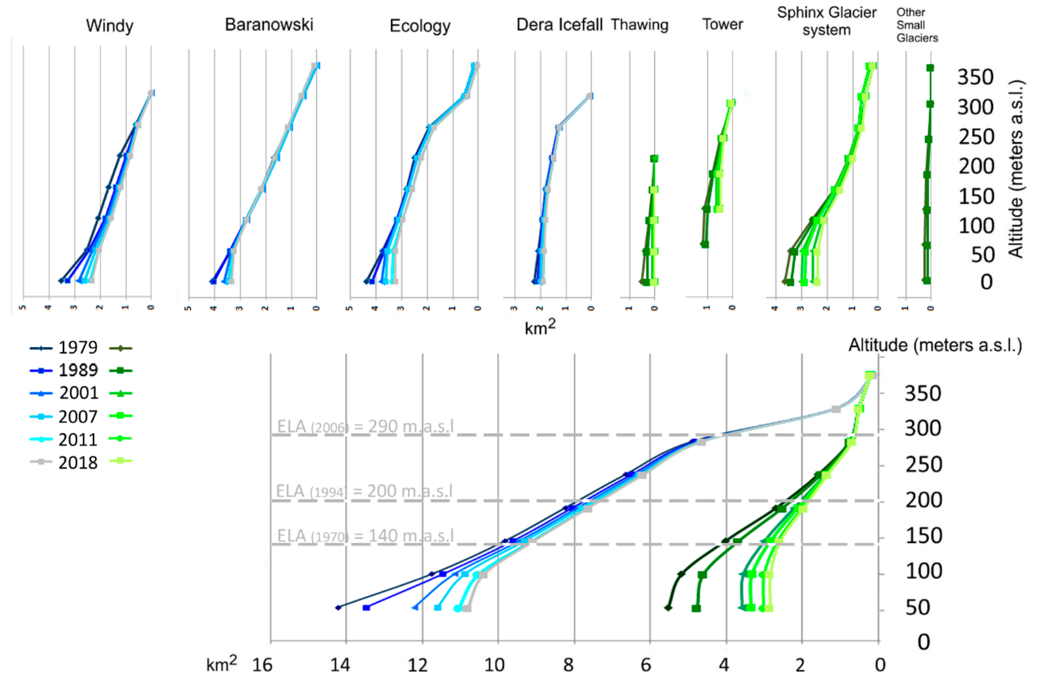
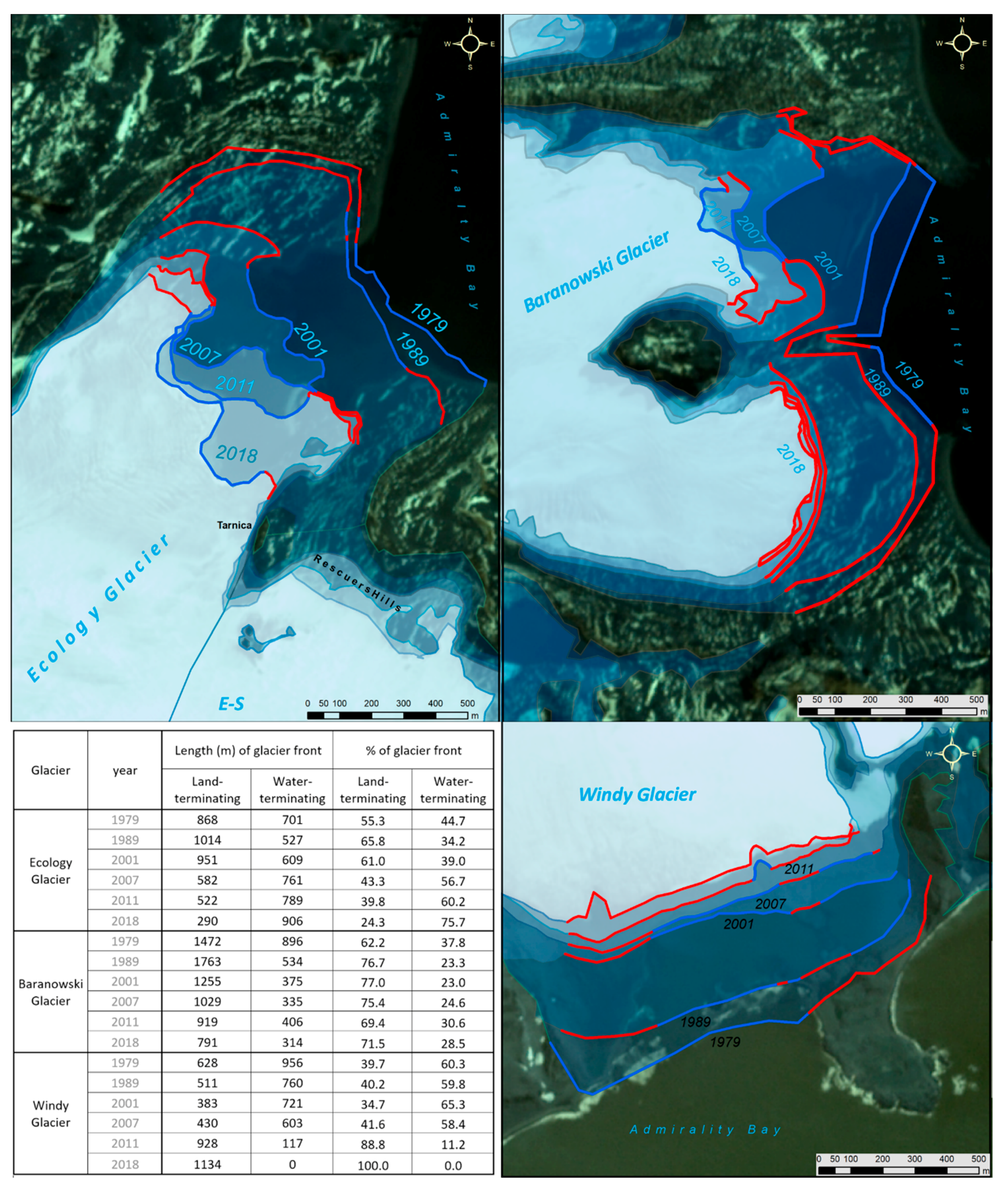
The process of deglaciation in the studied area has been observed since the 1950s, but until the 1980s, the rate of change was not significant to the ecosystem. The observed changes in glacier extent over the last three decades indicate an ongoing process of deglaciation throughout ASPA-128, with an average loss in the glaciated area of −0.277 km²/year for 1979–2011. In 1979, within the studied area, 19.8 km² was glaciated and 6.2 km² (31.3%) became ice-free in 2018. As a result, large ice-free areas have appeared along the glacier fronts. The convergent oscillation of the rate of glaciers retreat in the same time periods (for example, the fastest retreat in 1990s) demonstrates that the entire Warszawa Icefield glacial system responds rapidly to climate fluctuations and is sensitive to climate change. The important finding of our study is that glacier retreat between 1979 and 2011 in the eastern part of the Warszawa Icefield was increasing, with the exception of the period between 2001 and 2007 when the tempo was reduced. However, in the last 7 years, the glaciers’ retreat rates have clearly decreased.

(2)

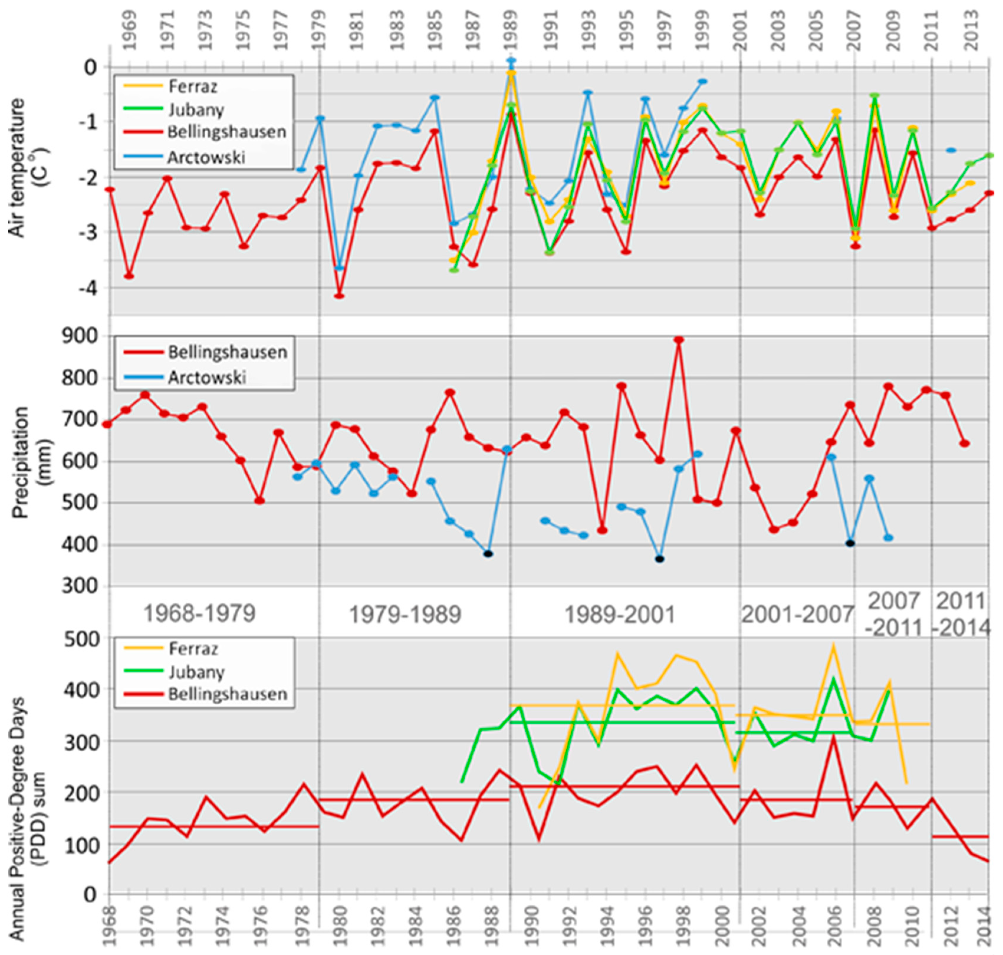
The PDD values well matched the observed retreat rates for the studied intervals and, therefore, the surface melting was interpreted to be the key contributor to glaciated area loss for land-terminating glaciers. The increase in PDD and the resulting ELA increase contributed to the degradation of small cirque glaciers located below 250 m a.s.l. in ASPA-128. The PPD sums act as the only analysed weather indicator that is correlated with the observed decline in the rate of glacier retreat in recent years (2011–2018).

(3)

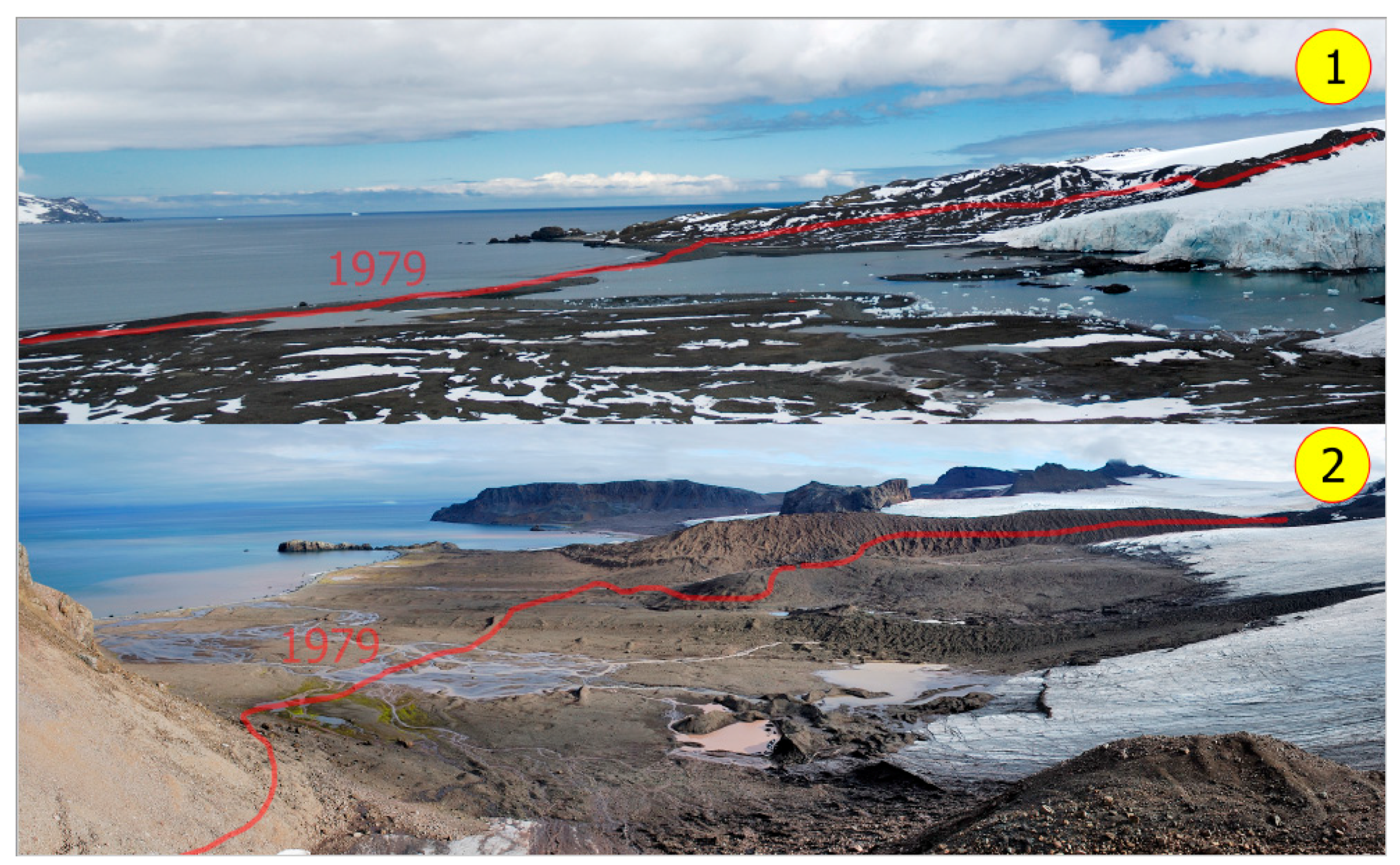
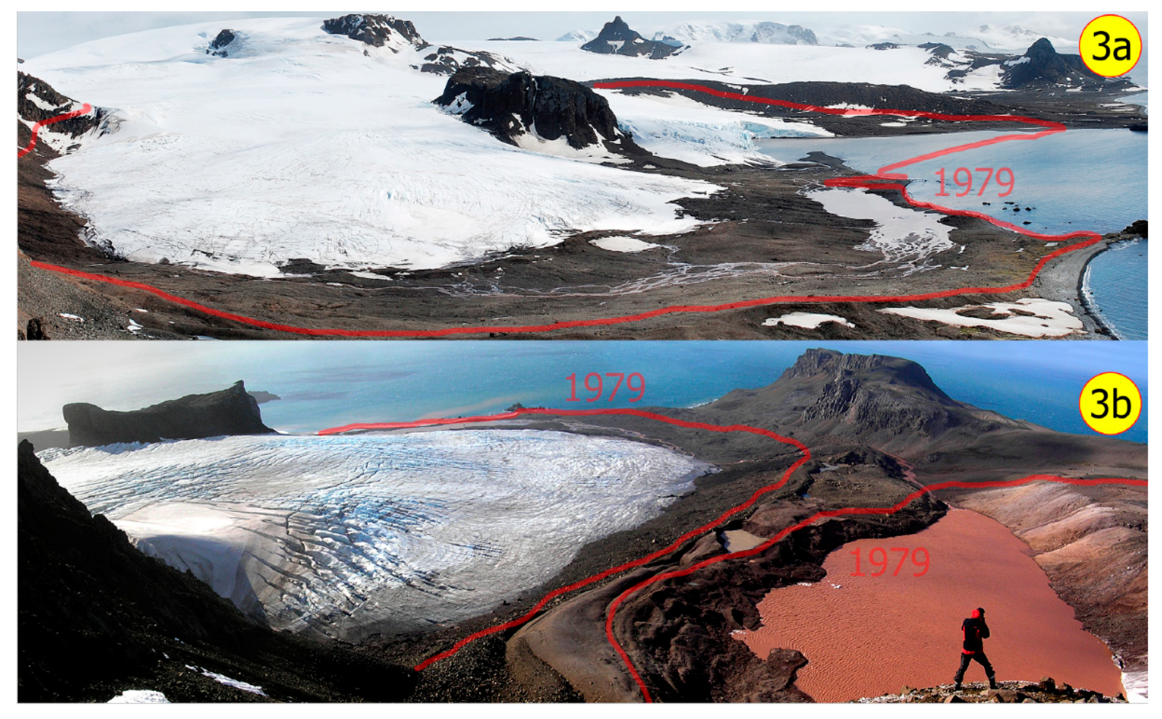
Large areas in ASPA-128 become ice-free between 1979–2018. These areas are colonized by plants and become nesting and resting areas for birds and sea mammals. Further studies and the monitoring of glacier changes should be continued in order to document the changes of the environment, which are affecting the land and marine ecosystems of Antarctica.

References

1. Kejna, M.; Araźny, A.; Sobota, I. Climatic change on King George Island in the years 1948–2011. Pol. Polar Res. 2013, 34, 213–235. [Google Scholar] [CrossRef] [Green Version]
2. Turner, J.; Colwell, S.R.; Marshall, G.J.; Lachlan-Cope, T.A.; Carleton, A.M.; Jones, P.D.; Lagun, V.; Reid, P.A.; Iagovkina, S. Antarctic climate change during the last 50 years. Int. J. Climatol. 2005, 25, 279–294. [Google Scholar] [CrossRef] [Green Version]
3. Marshall, G.J.; Lagun, V.; Lachlan-Cope, T.A. Changes in Antarctic Peninsula tropospheric temperatures from 1956–1999: A synthesis of observations and reanalysis data. Int. J. Climatol. 2002, 22, 291–310. [Google Scholar] [CrossRef]
4. Cook, A.J.; Fox, A.J.; Vaughan, D.G.; Ferrigno, J.G. Retreating glacier fronts on the Antarctic Peninsula over the past half-century. Science 2005, 308, 541–544. [Google Scholar] [CrossRef] [PubMed]
5. Cook, A.; Poncet, S.; Cooper, A.; Herbert, D.; Christie, D. Glacier retreat on South Georgia and implications for the spread of rats. Antarct. Sci. 2010, 22, 255–263. [Google Scholar] [CrossRef] [Green Version]
6. Angiel, P.J.; Dąbski, M. Lichenometric ages of the Little Ice Age moraines on King George Island and of the last volcanic activity on Penguin Island (West Antarctica). Geogr. Ann. Ser. A Phys. Geogr. 2012, 94, 395–412. [Google Scholar] [CrossRef]
7. Noble, H.M. Glaciological Observations at Admiralty Bay, King George Island in 1957–58. Br. Antarct. Surv. Bull. 1965, 5, 1–11. [Google Scholar]
8. Rückamp, M.; Braun, M.; Suckro, S.; Blindow, N. Observed glacial changes on the King George Island ice cap, Antarctica, in the last decade. Glob. Planet. Chang. 2011, 79, 99–109. [Google Scholar] [CrossRef]
9. Sobota, I.; Kejna, M.; Araźny, A. Short-term mass changes and retreat of the Ecology and Sphinx glacier system, King George Island, Antarctic Peninsula. Antarct. Sci. 2015, 27, 500–510. [Google Scholar] [CrossRef]
10. Simões, J.C.; Bremer, U.F.; Aquino, F.E.; Ferron, F.A. Morphology and variations of glacial drainage basins in the King George Island ice field, Antarctica. Ann. Glaciol. 1999, 29, 220–224. [Google Scholar] [CrossRef] [Green Version]
11. Simões, J.C.; Dani, N.; Bremer, U.F.; Aquino, F.E.; Arigony-Neto, J. Small cirque glaciers retreat on Keller Peninsula, Admiralty Bay, King George Island, Antarctica. Pesqui. Antart. Bras. 2004, 4, 49–56. [Google Scholar]
12. Pętlicki, M.; Sziło, J.; MacDonell, S.; Vivero, S.; Bialik, R.J. Recent Deceleration of the Ice Elevation Change of Ecology Glacier (King George Island, Antarctica). Remote Sens. 2017, 9, 520. [Google Scholar] [CrossRef]
13. Knap, W.H.; Oerlemans, J.; Cadée, M. Climate sensitivity of the ice cap of King George Island, South Shetland Islands, Antarctica. Ann. Glaciol. 1996, 23, 154–159. [Google Scholar] [CrossRef] [Green Version]
14. Bintanja, R. The local surface energy balance of the Ecology Glacier, King George Island Antarctica: Measurements and modelling. Antarct. Sci. 1995, 7, 315–325. [Google Scholar] [CrossRef]
15. Braun, M.; Saurer, H.; Vogt, S.; Simões, J.C.; Grossmann, H. The influence of large-scale atmospheric circulation on the surface energy balance of the King George Island ice cap. Int. J. Climatol. 2001, 21, 21–36. [Google Scholar] [CrossRef] [Green Version]
16. Olech, M. Responses of Antarctic tundra ecosystem to climate change and human activity. Pap. Glob. Chang. IGBP 2010, 17, 43–52. [Google Scholar] [CrossRef]
17. Olech, M.; Węgrzyn, M.; Lisowska, M.; Słaby, A.; Angiel, P.J. Contemporary Changes in vegetation of Polar Regions. Pap. Glob. Chang. 2011, 18, 35–51. [Google Scholar] [CrossRef]
18. Wolicka, D.; Zdanowski, M.K.; Żmuda-Baranowska, M.J.; Poszytek, A.; Grzesiak, J. Sulphate reducing activity detected in soil samples from Antarctica, Ecology Glacier forefield, King George Island. Pol. J. Microbiol. 2014, 63, 443–450. [Google Scholar] [PubMed]
19. Olech, M.; Chwedorzewska, K.J. Short Note: The first appearance and establishment of an alien vascular plant in natural habitats on the forefield of a retreating glacier in Antarctica. Antarct. Sci. 2011, 23, 153–154. [Google Scholar] [CrossRef] [Green Version]
20. Landsat Data Continuity Mission (LDCM). Available online: https://directory.eoportal.org/web/eoportal/satellite-missions/l/landsat-8-ldcm (accessed on 17 May 2018).
21. The Advanced Spaceborne Thermal Emission and Reflection Radiometer (ASTER). Available online: https://www.nasa.gov/feature/jpl/nasa-japan-make-aster-earth-data-available-at-no-cost (accessed on 17 May 2018).
22. USGS Earth Explorer. Available online: https://earthexplorer.usgs.gov/ (accessed on 17 May 2018).
23. Copernicus Programme Sentinel-2 Missions. Available online: https://sentinel.esa.int/web/sentinel/missions/sentinel-2 (accessed on 17 May 2018).
24. Planet Team. Planet Application Program Interface: In Space for Life on Earth. San Francisco, CA, USA, 2018. Available online: https://api.planet.com (accessed on 17 May 2018).
25. Downie, R.H. The Falkland Islands and Dependencies Aerial Survey Expedition (FIDASE) (1955–1957). In Encyclopedia of the Antarctic; Rifenburgh, B., Ed.; Routledge: New York, NY, USA, 2007; pp. 383–384. [Google Scholar]
26. Pudełko, R. Two new topographic maps for sites of scientific interest on King George Island, West Antarctica. Pol. Polar Res. 2008, 29, 291–297. [Google Scholar]
27. Braun, M.; Simões, J.C.; Vogt, S.; Bremer, U.F.; Blindow, N.; Pfender, M.; Saurer, H.; Aquino, F.E.; Ferron, F.A. An improved topographic database for King George Island: Compilation, application and outlook. Antarct. Sci. 2001, 13, 41–52. [Google Scholar] [CrossRef]
28. Goetzendorf-Grabowski, T.; Rodzewicz, M. Design of UAV for photogrammetric mission in Antarctic area. J. Aerosp. Eng. 2016, 231. [Google Scholar] [CrossRef]
29. Marsz, A.A.; Styszyńska, A. (Eds.) The main features of the climate region the Polish Antarctic Station H. Arctowski (West Antarctica, South Shetland Islands, King George Island); Wyższa Szkoła Morska: Gdynia, Poland; 264p. (In Polish)
30. Barrand, N.E.; Vaughan, D.G.; Steiner, N.; Tedesco, M.; Kuipers Munneke, P.; Van Den Broeke, M.R.; Hosking, S.J. Trends in Antarctic Peninsula surface melting conditions from observations and regional climate modeling. J. Geophys. Res. Earth Surf. 2013, 118, 315–330. [Google Scholar] [CrossRef] [Green Version]
31. Hall, D.K.; Riggs, G.A.; Salomonson, V.V. Development of methods for mapping global snow cover using moderate resolution imaging spectroradiometer data. Remote Sens. Environ. 1995, 54, 27–140. [Google Scholar] [CrossRef]
32. Naegeli, K.; Damm, A.; Huss, M.; Wulf, H.; Schaepman, M.; Hoelzle, M. Cross-Comparison of albedo products for glacier surfaces derived from airborne and satellite (Sentinel-2 and Landsat 8) optical data. Remote Sens. 2017, 9, 110. [Google Scholar] [CrossRef]
33. Battke, Z. Admiralty Bay, King George Island, 1:50,000 Scale; E. Romer State Cartographic Publishing House: Warsaw, Poland, 1990. [Google Scholar]
34. Pudełko, R. Topographic map of the SSSI No. 8, King George Island, West Antarctica. Pol. Polar Res. 2003, 24, 53–60. [Google Scholar]
35. Braun, M.; Goßmann, H. Ecological Studies chapter Climate change indications in the region of the Antarctic Peninsula. In Geoecology of Antarctic Ice-Free Coastal Landscapes; Springer: Berlin/Heidelberg, Germany, 2002; Volume 154, pp. 75–89. [Google Scholar]
36. Orheim, O.; Govorukha, L.S. Present-day glaciation in the South Shetland Islands. Ann. Glaciol. 1982, 3, 233–238. [Google Scholar] [CrossRef]
37. Ren, J.; Qin, D.; Petit, J.R.; Jouzel, J.; Wang, W.; Liu, C.; Wang, X.; Qian, S.; Wang, X. Glaciological studies on Nelson Island, South Shetland Islands, Antarctica. J. Glaciol. 1995, 41, 408–412. [Google Scholar] [CrossRef] [Green Version]
38. Braun, M.; Rau, F. Using a multi-year data archive of ERS SAR imagery for the monitoring of firn line positions and ablation patterns on the King George Island ice cap (Antarctica). The Workshop of EARSeL Special Interest Group: Remote Sensing of Land Ice and Snow. Dresden, Germany. EARSeL eProceedings 2000, 1, 281–291. [Google Scholar]
39. Laumann, T.; Reeh, N. Sensitivity to climate change of the mass balance of glaciers in southern Norway. J. Glaciol. 1993, 39, 656–665. [Google Scholar] [CrossRef]
40. Fox, A.J.; Cooper, A.P.R. Climate-change indicators from archival aerial photography of the Antarctic Peninsula. Ann. Glaciol. 1998, 27, 636–642. [Google Scholar] [CrossRef]
41. Winkelmann, R.; Levermann, A.; Martin, M.A.; Frieler, K. Increased future ice discharge from Antarctica owing to higher snowfall. Nature 2012, 492, 239–242. [Google Scholar] [CrossRef] [PubMed]
42. van Lipzig, N.P.M.; King, J.C.; Lachlan-Cope, T.A.; van den Broeke, M.R. Precipitation, sublimation and snow drift in the Antarctic peninsula region from a regional atmospheric model. J. Geophys. Res. 2004, 109, D24106. [Google Scholar] [CrossRef]
43. Rachlewicz, G. Mid-winter thawing in the vicinity of Arctowski Station, King George Island. Pol. Polar Res. 1997, 18, 15–24. [Google Scholar]
44. Angiel, P.J.; Potocki, M.; Biszczuk-Jakubowska, J. Characterization of weather conditions at H. Arctowski Station (South Shetland Island, Antarctica) in 2006, in comparison with historical observations. Misc. Geogr. 2010, 14, 5–11. [Google Scholar]
45. Rückamp, M.; Blindow, N.; Suckro, S.; Braun, M.; Humbert, A. Dynamics of the ice cap on King George Island, Antarctica: Field measurements and numerical simulations. Ann. Glaciol. 2010, 51, 80–90. [Google Scholar] [CrossRef]
46. Osmanoglu, B.; Braun, M.; Hock, R.; Navarro, F.J. Surface velocity and ice discharge of the ice cap on King George Island, Antarctica. Ann. Glaciol. 2013, 54, 111–119. [Google Scholar] [CrossRef] [Green Version]
47. Warren, C.R. Iceberg calving and the glaciomarine record. Prog. Phys. Geogr. 1992, 16, 253–282. [Google Scholar] [CrossRef]
48. Pritchard, H.D.; Vaughan, D.G. Widespread acceleration of tidewater glaciers on the Antarctic Peninsula. J. Geophys. Res. 2007, 112, F03S29. [Google Scholar] [CrossRef]
49. Korczak-Abshire, M.; Węgrzyn, M.; Angiel, P.J.; Lisowska, M. Pygoscelid penguins breeding distribution and population trends at Lions Rump rookery, King George Island. Pol. Polar Res. 2013, 34, 87–99. [Google Scholar] [CrossRef] [Green Version]
50. Hinke, J.T.; Trivelpiece, S.G.; Trivelpiece, W.Z. Adelie penguin (Pygoscelis adeliae) survival rates and their relationship to environmental indices in the South Shetland Islands, Antarctica. Pol. Biol. 2014, 37, 1797–1809. [Google Scholar] [CrossRef]
51. Pina, P.; Vieira, G.; Bandeira, L.; Mora, C. Accurate determination of surface reference data in digital photographs in ice-free surfaces of Maritime Antarctica. Sci. Total Environ. 2016, 573, 290–302. [Google Scholar] [CrossRef] [PubMed]
52. Funaki, M.; Higashino, S.I.; Sakanaka, S.; Iwata, N.; Nakamura, N.; Hirasawa, N.; Obara, N.; Kuwabara, M. Small unmanned aerial vehicles for aeromagnetic surveys and their flights in the South Shetland Islands, Antarctica. Pol. Sci. 2014, 8, 342–356. [Google Scholar] [CrossRef]
53. Fieber, K.D.; Mills, J.P.; Miller, P.E.; Clarke, L.; Ireland, L.; Fox, A.J. Rigorous 3D change determination in Antarctic Peninsula glaciers from stereo WorldView-2 and archival aerial imagery. Remote Sens. Environ. 2018, 205, 18–31. [Google Scholar] [CrossRef]
54. Zmarz, A.; Korczak-Abshire, M.; Storvold, R.; Rodzewicz, M.; Kedzierska, I. Indicator species population monitoring in Antarctica with UAV. Int. Arch. Photogramm. Remote Sens. Spat. Inf. Sci. 2015, 40, 189. [Google Scholar] [CrossRef]
Figure 1. The study area: (a) the location of King George Island in West Antarctica, (b) the location of the ASPA-128 and ASPA-151 on King George Island; glaciated areas indicated by light grey color, ice-free areas are in black; 1-Bellingshausen Station, 2-Arctowski Station, 3-Ferraz Station, 4-Jubany Station, 5-Fildes Peninsula, 6-Arctowski Icefield.
Remotesensing 10 00892 g001
Figure 2. The average air temperature, precipitation, and averages for the periods analysed in this paper. The trends are from the Arctowski (A, 1977–1999), Bellingshausen (B, 1968–2014), Jubany (J, 1986–2014), and Ferraz (F, 1986–2013) stations. All plots from the Arctowski Station are based on data from the Department of Antarctic Biology of Polish Academy of Sciences (Warsaw, Poland), the plots from the Bellingshausen Station are based on data from the Arctic and Antarctic Research Institute (Saint Petersburg, Russia), the plots from the Jubany and Ferraz stations from the READER (Reference Antarctic Data for Environmental Research)—a project of the Scientific Committee on Antarctic Research, http://www.scar.org [2]; the annual Positive Degree-Days (PDD) sums plots from Jubany (J) and Ferraz (F) stations from Barrand et al. [30].
Remotesensing 10 00892 g002
Figure 3. The detection accuracy of the marginal zone of the Tower glacier. (A) the Landsat image with a resolution of 30 m; (B) the image of Normalised Difference Snow Index (NDSI) with a resolution of 30 m; (C) the image of pan-Normalised Difference Snow Index (panNDSI) with a resolution of 15 m; (D) the Planet satellite image with a resolution of 3 m; (E) the margin zone buffer with a width of 30 m; (F) the accuracy of ice border detection.
Remotesensing 10 00892 g003
Figure 4. The Baranowski Glacier (tidewater glacier) and Sphinx Glacier—part Sb (land-terminating glacier). The comparison of the PlanetScope satellite image (2018) with BAS (1956), Polish aerial photos (1979), and Geo-Eye1 (2011).
Remotesensing 10 00892 g004
Figure 5. The changes in glacier coverage during periods of 1979–1989, 1989–2001, 2001–2007, 2007–2011, and 2011–2018 in ASPA-128. The altitudes of the lowest (140 m a.s.l.) and the highest (290 m a.s.l.) reported Equilibrium-Lines Altitude (ELA) are marked on the map. Glacier zones: Dera Icefall, Wróbel Glacier (Xa), Wróbel-Italian Glacier (Xb), Ecology Glacier, Ecology-Sphinx (E–S), Rescuers Hills (R), Sphinx Glacier (Sa), Sphinx-Czajkowski Glacier (Sb), Baranowski Glacier, Tower Glacier, Thawing Glacier (Ta), Windy Glacier. The location of the photographs are shown in Appendix A Figure A2, Figure A3 and Figure A4 and their directions were marked in the yellow circles.
Remotesensing 10 00892 g005
Figure 6. The cumulative chart of the glaciers’ retreat ratio for chosen intervals of altitude and analysed periods (L: land-terminating glaciers; T: tidewater glaciers) based on Table A1 (see Appendix A). The changes of average air temperature, precipitation, and PPD sums in the analysed periods were imposed (based on data presented on the Figure 2).
Remotesensing 10 00892 g006
Figure 7. The changes in the altitude profiles of the studied glaciers. The land-terminating glaciers are in green and the tidewater glaciers are in blue. For simplicity, the zones Xa and Xb were grouped together as ‘Other Small Glaciers’ and the zones E-S, R, Sa, and Sb were grouped together as ‘Sphinx Glacier system’.
Remotesensing 10 00892 g007