Measurement-Based Adaptation Protocol with Quantum Reinforcement Learning in a Rigetti Quantum Computer


1
Department of Physical Chemistry, University of the Basque Country UPV/EHU, Apartado 644, 48080 Bilbao, Spain
2
IKERBASQUE, Basque Foundation for Science, Maria Diaz de Haro 3, 48013 Bilbao, Spain
3
International Center of Quantum Artificial Intelligence for Science and Technology (QuArtist) and Physics Department, Shanghai University, Shanghai 200444, China
4
IQM, 80336 Munich, Germany
5
Departamento de Física Atómica, Molecular y Nuclear, Universidad de Sevilla, 41080 Sevilla, Spain
*
Author to whom correspondence should be addressed.
Quantum Rep. 2020, 2(2), 293-304; https://doi.org/10.3390/quantum2020019
Submission received: 31 March 2020
/
Revised: 6 May 2020
/
Accepted: 15 May 2020
/
Published: 19 May 2020
(This article belongs to the Special Issue Exclusive Feature Papers of Quantum Reports)
Abstract
:We present an experimental realisation of a measurement-based adaptation protocol with quantum reinforcement learning in a Rigetti cloud quantum computer. The experiment in this few-qubit superconducting chip faithfully reproduces the theoretical proposal, setting the first steps towards a semiautonomous quantum agent. This experiment paves the way towards quantum reinforcement learning with superconducting circuits.
1. Introduction
Quantum machine learning [1,2,3,4,5,6,7,8,9,10,11,12,13,14,15,16,17,18,19,20,21,22,23,24,25,26,27,28,29] is a field of research that has raised much attention in the past few years, especially for the expectation that it may enhance the machine learning calculations in current and future technology. The machine learning field, inside artificial intelligence, is divided into three main areas: supervised learning, unsupervised learning and reinforcement learning [30]. The first two rely on training the system via labelled or unlabelled data, respectively. Moreover, the third one considers an intelligent agent that interacts with its outer world, the environment, gathering information from it, as well as acting on it, being employed, e.g., in robotics. In each learning iteration, the agent decides a strategy, or policy, on the best action to take, depending on its past history and goal oriented. Reinforcement learning can be considered as the most similar way in which human beings learn, via interactions with their outer world.
Among the protocols being developed in quantum machine learning, the ones based on quantum reinforcement learning will enable the future deployment of semiautonomous quantum agents, which may produce significant advances in quantum computation and artificial intelligence [1,2,25,26,27,28,29]. Already some possible speedups when considering quantum agents have been suggested [25], while other interesting aspects of quantum reinforcement learning are related to quantum systems autonomously learning quantum data [1].
In this article, we implement a protocol for measurement-based adaptation with quantum reinforcement learning, proposed in [1], in an 8-qubit cloud quantum computer provided by Rigetti. The experimental results have a good agreement with the theoretical expectations, establishing a plausible avenue for the future development of semiautonomous quantum agents. We point out that further efforts in experimental quantum machine learning, both in superconducting circuits [31] and in quantum photonics [32], are being pursued.
2. Results
2.1. Measurement-Based Adaptation Protocol with Quantum Reinforcement Learning
We review the protocol of [1], which we subsequently implement in the Rigetti cloud quantum computer. The aim of this algorithm is to adapt a quantum state to a reference unknown state via successive measurements. Many identical copies of the reference state are needed for this protocol and, after each measurement, which destroys the state, more information about it is obtained. The system that we consider is composed of the following parts:
- The environment system (E) contains the reference state copies.
- The register (R) interacts with E and obtains information from it.
- The agent (A) is adapted by digital feedback depending on the outcome of the measurement of the register.
Let us assume that we know the state of a quantum system called agent and that many copies of an unknown quantum state called environment are provided. Let us also consider an auxiliary system called register that interacts with E. Thus, we extract information from E by measuring R and use the result as an input for a reward function (RF).
Subsequently, we perform a partially-random unitary transformation on A, which depends on the output of the RF.
Let us present the simplest case in which each subsystem is described by a qubit state: Agent , Register and Environment .
Therefore, the initial state is,
Then, we apply a CNOT gate with E as control and R as target (policy) to obtain information from E, namely
Secondly, we measure the register qubit in the basis with probability or of obtaining the state or , respectively. Depending on the result of the measurement, we either do nothing if the result is , since it means that we collapse E into A, or perform a partially-random unitary operator on A, if the result is This unitary transformation (action) is given by
where is the kth spin component; and are random angles; and are random numbers. The range of the random numbers is .
Now, we initialise the register qubit state and use a new copy of the environment obtaining the following initial state for the second iteration,
with where is the outcome of the measurement, and we call .
Later, we define the RF as
As we can see, the exploration range of the kth iteration, , is modified by when the outcome of the iteration was and by , when it was . Here, we chose , , with being a constant.
We define the value function (VF) in this protocol as the value of after many iterations assuming that , i.e., that the agent converges to the environment state.
In the kth iteration of the protocol, we assume that the system starts in the following state,
where , , and the accumulated rotation operator is,
with .
Then, we perform the gate ,
and measure R, with probabilities and , for the outcomes and , respectively. Finally, we update the reward function, , for the next iteration.
2.2. Experimental Setup: Rigetti Forest Cloud Quantum Computer
Cloud quantum computers are dedicated quantum processors operated by users logged through the Internet (cloud). Although D-Wave Systems, Inc. [33] was among the first companies to commercialise quantum computers in 2011, it was not until the arrival of IBM Quantum Experience [34] in May 2016 that there was a quantum computer openly available in the cloud. Approximately one year later, in June 2017, Californian company Rigetti Computing [35] announced the availability of a cloud quantum computing platform. This last quantum platform is the one that we used in this work, because of convenience of their web interface to implement our protocol with feedback. In the past year, Rigetti built a brand new processor of 8 qubits called 8Q-Agave: this is the chip we employed. An advantage of this device is that one does not have to adapt the algorithm to the topology of the system. The compiler does it for us. In particular, it is the possibility of defining quantum gates in matrix form that makes the adaptation significantly simpler. Among other features, Rigetti Forest offers the possibility of simulating the experiments in their quantum virtual machine (QVM).
Python-Implemented Algorithm
In this section, we explain how the algorithm of Section 2.1 is adapted to be implemented in Rigetti simulator and quantum processor. Firstly, we must initialise some variables and constants to correctly perform the first iteration,
- Reward and punishment ratios: and .
- Exploration range: .
- The unitary transformation matrices: .
- Partially-random unitary operator: .
- Initial values of the random angles: . Makes for the first iteration.
- Initial value of the iteration index: .
- Number of iterations: N.
The algorithm is composed of the following steps,
- Step 1: While , go to Step 2.
- Step 2: If
- Step 3: First quantum algorithm.First, we define the agent, environment and register qubits as,and act upon the environment,Then, we haveWe apply the policyand measure the register qubit storing the result in .
- Step 4: Second quantum algorithm.Subsequently, we act with on the agent qubit in order to approach it to the environment state, :Afterwards, we measure this qubit and store the result in a classical register array. We repeat Step 4 a total of 8192 times to determine the state created after applying .
- In this last step, we apply the reward function,and increase the iteration index by one after it: . Go to Step 1.
2.3. Experimental Results of Quantum Reinforcement Learning with the Rigetti Cloud Quantum Computer
In this section, we describe the experimental results with the Rigetti cloud quantum computer of the measurement-based adaptation protocol of [1].
The algorithm has been proved for six different initial states of the environment. The states contain different weights of the quantum superpositions of and states, as well as different complex relative phases, to illustrate the performance of the protocol in a variety of situations. These states are the following,
Hereunder, we plot the exploration range, , and the fidelity, which we define in Equation (26), in terms of the total number of iterations. The results obtained using the 8Q-Agave chip of Rigetti are shown with the corresponding ideal simulation with the Rigetti quantum virtual machine, which includes no noise. We point out that each of the experimental plots in this article contains a single realisation of the experiment, given that, in the adaptation protocol, single instances are what are relevant instead of averages. This is due to the fact that the successive measurements influence the subsequent ones and are influenced by the previous ones, in each experiment, in order for the agent to adapt to the environment. This has as a consequence the fact that the theory curve and the experimental curve for each example match qualitatively but not totally quantitatively, as they are both probabilistic. On the other hand, when the exploration range converges to zero we always observe convergence to a large final fidelity. The blue solid line represents the real experiment result while the red dashed-dotted one corresponds to the ideal simulation. It is also worth mentioning that after doing many experiments with the ideal and real simulators for different values of the parameter , we fixed it to . We found it to yield a balanced exploration–exploitation ratio. The exploration–exploitation balance is a feature of reinforcement learning, where the optimal strategy must deal with exploring enough new possibilities while at the same time exploiting the ones that work best [30].
To begin with, let us have a look at Figure 1, in which the environment state is . It shows the exploration ratio, and the fidelity as defined in Equation (26) in terms of the number of iterations. As we can see, 140 iterations are enough for to take a value of almost zero. It is a good example of a balanced exploration versus exploitation ratio, that is, the exploration ratio decreases making continuous peaks. Each of them represents an exploration stage where increases at the same time that the fidelity changes significantly. These changes might bring a positive result, such that the agent receives a reward, which means that decreases, or a punishment and it keeps increasing. Thus, the fidelity is not constant and it does not attain a constant value of around 95% until it has done 100 iterations. In this case real and ideal experiments yield a similar result. It is true that the ideal decreases more smoothly and quickly than the real one. However, the values of the fidelity after 130 iterations are practically the same.
In our calculations, we employ a classical measure of the fidelity. The reason to use the classical fidelity, and not the quantum version, is the reduction of needed resources in the experiments. We cannot make full quantum state tomography as it is exponentially hard. Therefore, the definition used in the algorithm is,
for one-qubit measurements. Here, and stand for the probability of obtaining or as an outcome when measuring the real qubit and and are the same probabilities for the corresponding theoretical qubit state that we expect. This fidelity coincides at lowest order with the fully quantum one, illustrating the convergence of the protocol for a large number of iterations.
Let us continue with the discussion focussing on Figure 2. In this experiment, the algorithm has to take the agent from the state to the environment state which is closer to one than to zero (0.6 is the probability of getting as an outcome when measuring the environment). Bearing this in mind, it seems reasonable that 70 iterations are not enough for to reach a value below 2, in the real case. Apart from this, despite achieving a value above 99% of fidelity in fewer than 20 iterations, the exploration still continues. Consequently, the agent drops from its current state to one further from .
In general, we notice a clear relationship between how smooth the line is and how constant the fidelity remains. Indeed, the exploration ratio decreases smoothly from fewer than 20 iterations to fewer than 40. In this range, the fidelity does not change because the agent is being rewarded. The price to pay for not exploring at so early stages of the learning is that the convergence of the delta is produced for a larger number of iterations than in other experiments. After 140 iterations, we see that the convergence of is not guaranteed, namely, in the real experiment, it has a value above 1. Regarding the ideal simulation result, we draw the conclusion that fewer than 20 iterations could be enough to converge to the environment state with fidelity larger than 99.9% and, what is more, remaining on the same state until the exploration range has converged to zero (see inset in Figure 2).
In third place, we have the environment state . The results obtained using this initial state of the environment are presented in Figure 3 and Figure 4. Unlike the previous examples, we do not compare the ideal theory and real experiments, which have similarly good agreement. Instead, we contrast two different real experiment outcomes. In this way, we can show how even for the same experiment, i.e., initial state of the environment, the algorithm can experience different behaviours. In both cases, goes to zero and the fidelity reaches a constant value above 94% in the first case and 99% in the second one. However, this convergence is achieved in two different ways. On the one hand, we observe that exploitation predominates over exploration (see Figure 4), except for several spots where the algorithm keeps exploring new options. Then, as the initial fidelity is larger than 90%, the state of the agent converges to the environment with fewer than 70 iterations. On the other hand, when exploration is more important (as shown in Figure 3) the fidelity is erratic, changing from low to high values. Moreover, it takes longer for to converge and for the fidelity to be stabilised—more than 80 iterations.
Let us focus just on the first stages of the learning process, for fewer than 40 iterations. Comparing both experiments, we see that, in the first case, it starts exploring from the very beginning; thus, with fewer than 20 iterations, the fidelity takes a value above 99.6%. In the other case, there is more exploitation at the beginning and around 25 iterations are required to reach a fidelity of 99%.
Among the six states that we have chosen, this is the one in which agent and environment are the closest. Nevertheless, 70 iterations are not enough to reach a value of below 1. Thus, we can state that a smaller distance in the Bloch sphere between agent and environment does not imply in general a faster learning.
Let us analyse now Figure 5. This state is again the most asymmetric case along with the previous one. However, unlike the previous experiment, this one begins with the lowest value of fidelity. The environment state is the farthest one to the initial agent state , with just a probability of 0.25 of achieving this outcome (zero) when measuring the environment. Therefore, as might be expected, the algorithm is still exploring after 70 iterations rather than exploiting the knowledge it has already acquired from the environment. It is also proved that fewer than 100 iterations can be enough to reach a value of below 1. Then, in this case, it is proved that the agent has already converged to a state with fidelity larger than 97%. It is also remarkable how, in this case, with fewer than 10 iterations, the fidelity has attained a value larger than 99%. However, as the delta had not converged yet, it goes out of this value later, exploring again. Once again, as a general rule, we can see that the algorithm is exploring for all the iterations. To explore is a synonym of changing fidelity, while, whenever the delta decreases smoothly, the fidelity remains constant. With this result, we wanted to show how sometimes the real experiment converged more quickly, e.g., with just nine iterations, to the environment state. On the top of that, the exploration range also went to zero more quickly than the ideal experiment. Nevertheless, the value of fidelity when has converged is exactly the same in both cases.
We analyse now the most symmetric cases, where the environment is prepared in a uniform superposition with a relative phase between both states. The experiment chosen to highlight here (see Figure 6) is the one in which the fidelity reaches a constant value above 99.9% in fewer than 40 iterations. The corresponding evolves with a good balance between exploration and exploitation until reaching a point where it does not explore anymore and decreases very smoothly. Comparing it to the ideal case, we notice two opposing behaviours: the ideal case makes a larger exploration at the beginning which yields a larger constant value of the fidelity with fewer than 20 iterations, whereas the real system needs almost 40 iterations to get to this point. On the other hand, in the real experiment, there is a larger learning stage from 0 to 40 iterations. Thus, in this particular case, the exploration ratio diminishes more quickly in the real experiment for a large number of iterations. It happens because of the larger value of attained in the ideal experiment.
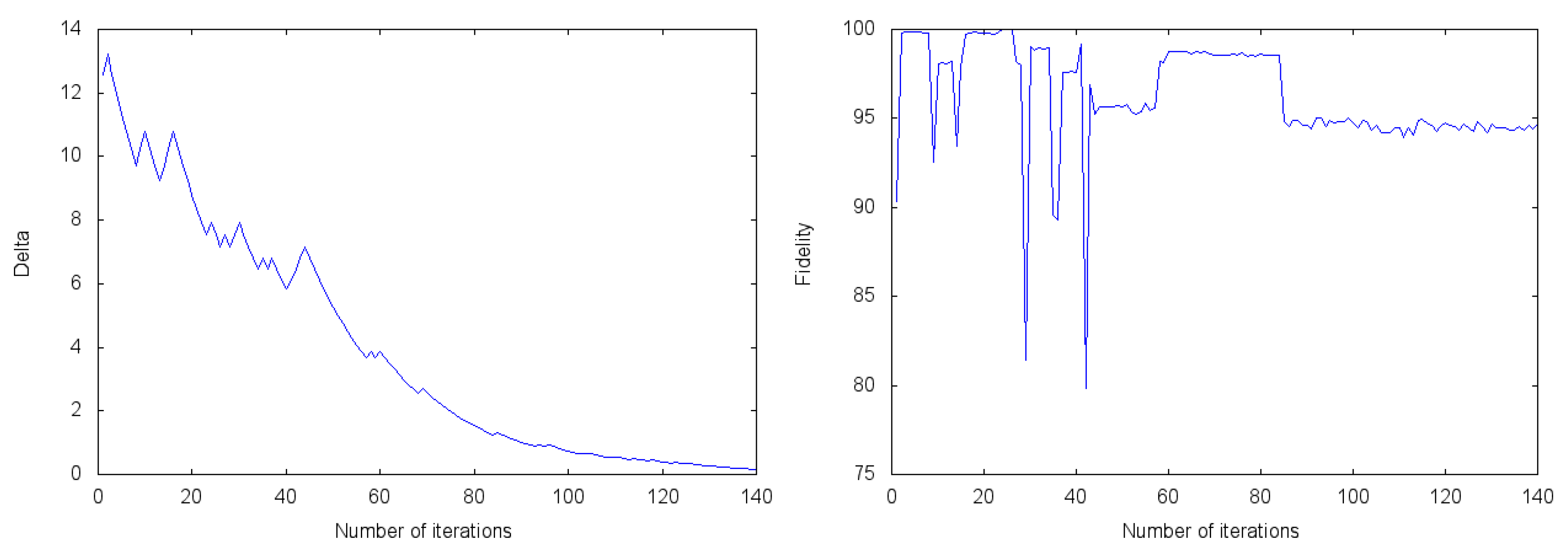
Finally, in this second symmetric case , there are no relative phases between the states of the computational basis. This experiment is very rich in phenomena and exemplifies very well how the algorithm works. Figure 7 shows clearly the fast increase of the fidelity until reaching values above 99.9% with just nine iterations. Initially, there is an exploration stage that makes the fidelity grow up to 99.9% with just nine iterations. At the same time, the exploration range, , grows, making two consecutive peaks and then it decreases smoothly, while the fidelity remains constant. Subsequently, there are a couple of exploration peaks that make the fidelity oscillate. Now, after a few iterations where the fidelity decreases smoothly, we come to a third and most important exploration phase where we observe how the fidelity has an increasing tendency. It suffices to check that the subsequent minima of the fidelity take larger and larger values. Such an amount of exploration has as a long-term reward a fidelity of 99.99% after fewer than 70 iterations. However, the exploration range is still large and leaves room for trying new states which make the fidelity drop again. Finally, the algorithm is able to find a good exploration-exploitation balance which makes the fidelity increase and remain constant with values above 99.5%. On the top of that, the exploration range goes progressively to zero. The ideal experiment is an excellent example of how quickly the algorithm could reach a high fidelity above 99.9% and also guarantee the convergence of . In this way, once the exploration range has become so small, it is assured that the agent does not go to another state. In other words, it is proved that the agent has definitely converged to the environment to a large fidelity.
In Table 1, we sort some results of the experiments run in Rigetti 8Q-Agave cloud quantum computer from larger to smaller value of the fidelity. As we can see, is close to 100% in most of the experiments when the exploration ratio is approaching zero. Thus, we are succeeding in adapting the agent to the environment state. From these data, we can also draw the conclusion that the convergence of the agent to the environment state is guaranteed whenever . We did not find any case where the exploration range is close to zero and the fidelity below 90%.
3. Discussion
In this study, we performed the implementation of the measurement-based adaptation protocol with quantum reinforcement learning of [1]. Consistently with it, we checked that indeed the fidelity increases reaching values over 90% with fewer than about 30 iterations in real experiments. We did not observe any case where and . Thus, to a large extent, the protocol succeeds in making the agent converge to the environment. If we wanted to apply this algorithm to any subroutine, it would be possible to track the evolution of the exploration range and deduce from it the convergence of the agent to the environment. This is because the behaviour of has proven to be closely related to the fidelity performance.
We can conclude that there is still a long way to be travelled until the second quantum revolution gives rise to well-established techniques of quantum machine learning in the lab. However, this work is encouraging since it sows the seeds for turning quantum reinforcement learning into a reality, and the future implementation of semiautonomous quantum agents.
We point out that another implementation of [1] in a different platform, namely quantum photonics, has been recently achieved, in parallel to this work [36]. The quantum photonics platform is more suited to quantum communication, while the current one, superconducting circuits, is more suited to quantum computation. On the other hand, there are interesting efforts for building quantum computers based on quantum photonics that exploit quantum machine learning techniques [32]. The importance of these two experiments of the proposal in [1] is the realisation that this proposal works well irrespective of the quantum platform in which it is implemented. Both experiments are complementary and it is valuable to show their good performance for different quantum technologies. The impact of quantum machine learning, and in particular, quantum reinforcement learning, in industry could be large in the short to mid term, and companies such as Xanadu [32], D-Wave [33], IBM [34] and Rigetti [35] are strongly investing on these efforts.
Author Contributions
J.O.-S. wrote the code and performed the experiments and simulations with Rigetti Forest. J.O.-S., J.C., E.S. and L.L. designed the protocol, analysed the results, and wrote the manuscript. All authors have read and agree to the published version of the manuscript.
Funding
J.C. acknowledges the support from Juan de la Cierva grant IJCI-2016-29681. We also acknowledge funding from Spanish Government PGC2018-095113-B-I00 (MCIU/AEI/FEDER, UE) and Basque Government IT986-16. This material is also based upon work supported by the projects OpenSuperQ and QMiCS of the EU Flagship on Quantum Technologies, FET Open Quromorphic, Shanghai STCSM (Grant No. 2019SHZDZX01-ZX04) and by the U.S. Department of Energy, Office of Science, Office of Advanced Scientific Computing Research (ASCR) quantum algorithm teams program, under field work proposal number ERKJ333.
Acknowledgments
The authors acknowledge the use of Rigetti Forest for this work. The views expressed are those of the authors and do not reflect the official policy or position of Rigetti, or the Rigetti team. We thank I. Egusquiza for useful discussions.
Conflicts of Interest
The authors declare no competing interests.
References
- Albarrán-Arriagada, F.; Retamal, J.C.; Solano, E.; Lamata, L. Measurement-based adaptation protocol with quantum reinforcement learning. Phys. Rev. A 2018, 98, 042315. [Google Scholar] [CrossRef] [Green Version]
- Albarrán-Arriagada, F.; Retamal, J.C.; Solano, E.; Lamata, L. Reinforcement learning for semi-autonomous approximate quantum eigensolver. Mach. Learn. Sci. Technol. 2020, 1, 015002. [Google Scholar] [CrossRef]
- Harrow, A.W.; Hassidim, A.; Lloyd, S. Quantum algorithm for linear systems of equations. Phys. Rev. Lett. 2009, 103, 150502. [Google Scholar] [CrossRef] [PubMed]
- Wiebe, N.; Braun, D.; Lloyd, S. Quantum algorithm for data fitting. Phys. Rev. Lett. 2012, 109, 050505. [Google Scholar] [CrossRef] [Green Version]
- Lloyd, S.; Mohseni, M.; Rebentrost, P. Quantum algorithms for supervised and unsupervised machine learning. arXiv 2013, arXiv:1307.0411. [Google Scholar]
- Rebentrost, P.; Mohseni, M.; Lloyd, S. Quantum support vector machine for big data classification. Phys. Rev. Lett. 2014, 113, 130503. [Google Scholar] [CrossRef]
- Wiebe, N.; Kapoor, A.; Svore, K.M. Quantum algorithms for nearest-neighbor methods for supervised and unsupervised learning. Quantum Inf. Comput. 2015, 15, 316. [Google Scholar]
- Lloyd, S.; Mohseni, M.; Rebentrost, P. Quantum principal component analysis. Nat. Phys. 2014, 10, 631. [Google Scholar] [CrossRef] [Green Version]
- Lau, H.K.; Pooser, R.; Siopsis, G.; Weedbrook, C. Quantum machine learning over infinite dimensions. Phys. Rev. Lett. 2017, 118, 080501. [Google Scholar] [CrossRef] [Green Version]
- Schuld, M.; Sinayskiy, I.; Petruccione, F. An introduction to quantum machine learning. Contemp. Phys. 2015, 56, 172. [Google Scholar] [CrossRef] [Green Version]
- Adcock, J.; Allen, E.; Day, M.; Frick, S.; Hinchli, J.; Johnson, M.; Morley-Short, S.; Pallister, S.; Price, A.; Stanisic, S. Advances in quantum machine learning. arXiv 2015, arXiv:1512.02900. [Google Scholar]
- Dunjko, V.; Taylor, J.M.; Briegel, H.J. Quantum-enhanced machine learning. Phys. Rev. Lett. 2016, 117, 130501. [Google Scholar] [CrossRef] [PubMed] [Green Version]
- Dunjko, V.; Briegel, H.J. Machine learning & artificial intelligence in the quantum domain: A review of recent progress. Rep. Prog. Phys. 2018, 81, 074001. [Google Scholar] [PubMed] [Green Version]
- Biamonte, J.; Wittek, P.; Pancotti, N.; Rebentrost, P.; Wiebe, N.; Lloyd, S. Quantum machine learning. Nature 2017, 549, 195. [Google Scholar] [CrossRef]
- Lamata, L. Quantum machine learning and quantum biomimetics: A perspective. arXiv 2020, arXiv:2004.12076. [Google Scholar]
- Biswas, R.; Jiang, Z.; Kechezhi, K.; Knysh, S.; Mandrà, S.; O’Gorman, B.; Perdomo-Ortiz, A.; Petukhov, A.; Realpe-Gómez, J.; Rieffel, E.; et al. A NASA perspective on quantum computing: Opportunities and challenges. Parallel Comput. 2017, 64, 81. [Google Scholar] [CrossRef] [Green Version]
- Perdomo-Ortiz, A.; Benedetti, M.; Realpe-Gómez, J.; Biswas, R. Opportunities and challenges for quantum-assisted machine learning in near-term quantum computers. Quantum Sci. Technol. 2018, 3, 030502. [Google Scholar] [CrossRef] [Green Version]
- Perdomo-Ortiz, A.; Feldman, A.; Ozaeta, A.; Isakov, S.V.; Zhu, Z.; O’Gorman, B.; Katzgraber, H.G.; Diedrich, A.; Neven, H.; de Kleer, J.; et al. Readiness of quantum optimization machines for industrial applications. Phys. Rev. Appl. 2019, 12, 014004. [Google Scholar] [CrossRef] [Green Version]
- Sasaki, M.; Carlini, A. Quantum learning and universal quantum matching machine. Phys. Rev. A 2002, 66, 022303. [Google Scholar] [CrossRef] [Green Version]
- Benedetti, M.; Realpe-Gómez, J.; Biswas, R.; Perdomo-Ortiz, A. Quantum-Assisted Learning of Hardware-Embedded Probabilistic Graphical Models. Phys. Rev. X 2017, 7, 041052. [Google Scholar] [CrossRef] [Green Version]
- Benedetti, M.; Realpe-Gómez, J.; Perdomo-Ortiz, A. Quantum-assisted helmholtz machines: A quantum-classical deep learning framework for industrial datasets in near-term devices. Quantum Sci. Technol. 2018, 3, 034007. [Google Scholar] [CrossRef] [Green Version]
- Aïmeur, E.; Brassard, G.; Gambs, S. Quantum speed-up for unsupervised learning. Mach. Learn. 2013, 90, 261. [Google Scholar] [CrossRef] [Green Version]
- Melnikov, A.A.; Nautrup, H.P.; Krenn, M.; Dunjko, V.; Tiersch, M.; Zeilinger, A.; Briegel, H.J. Active learning machine learns to create new quantum experiments. Proc. Natl. Acad. Sci. USA 2018, 115, 1221. [Google Scholar] [CrossRef] [PubMed] [Green Version]
- Alvarez-Rodriguez, U.; Lamata, L.; Escandell-Montero, P.; Martín-Guerrero, J.D.; Solano, E. Supervised Quantum Learning without Measurements. Sci. Rep. 2017, 7, 13645. [Google Scholar] [CrossRef]
- Paparo, G.D.; Dunjko, V.; Makmal, A.; Martin-Delgado, M.A.; Briegel, H.J. Quantum Speedup for Active Learning Agents. Phys. Rev. X 2014, 4, 031002. [Google Scholar] [CrossRef]
- Lamata, L. Basic protocols in quantum reinforcement learning with superconducting circuits. Sci. Rep. 2017, 7, 1609. [Google Scholar] [CrossRef] [Green Version]
- Cárdenas-López, F.A.; Lamata, L.; Retamal, J.C.; Solano, E. Multiqubit and multilevel quantum reinforcement learning with quantum technologies. PLoS ONE 2018, 13, e0200455. [Google Scholar] [CrossRef]
- Dong, D.; Chen, C.; Li, H.; Tarn, T.J. Quantum reinforcement learning. IEEE Trans. Syst. Man Cybern. Part B (Cybern.) 2008, 38, 1207–1220. [Google Scholar] [CrossRef] [Green Version]
- Crawford, D.; Levit, A.; Ghadermarzy, N.; Oberoi, J.S.; Ronagh, P. Reinforcement learning using quantum Boltzmann machines. Quant. Inf. Comput. 2018, 18, 51. [Google Scholar]
- Russell, S.; Norvig, P. Artificial Intelligence: A Modern Approach; Prentice Hall: Upper Saddle River, NJ, USA, 1995. [Google Scholar]
- Ristè, D.; Silva, M.P.D.; Ryan, C.A.; Cross, A.W.; Córcoles, A.D.; Smolin, J.A.; Gambetta, J.M.; Chow, J.M.; Johnson, B.R. Demonstration of quantum advantage in machine learning. NPJ Quantum Inf. 2017, 3, 16. [Google Scholar] [CrossRef]
- Quantum Computing Powered by Light. Available online: https://www.xanadu.ai (accessed on 16 May 2020).
- The Quantum Cloud Service Built for Business. Available online: https://www.dwavesys.com/home (accessed on 16 May 2020).
- Quantum Computing. Available online: https://www.research.ibm.com/ibm-q/ (accessed on 16 May 2020).
- Think Quantum. Available online: https://www.rigetti.com (accessed on 16 May 2020).
- Yu, S.; Albarrán-Arriagada, F.; Retamal, J.C.; Wang, Y.-T.; Liu, W.; Ke, Z.-J.; Meng, Y.; Li, Z.-P.; Tang, J.-S.; Solano, E.; et al. Reconstruction of a Photonic Qubit State with Quantum Reinforcement Learning. Adv. Quantum Technol. 2019, 2, 1800074. [Google Scholar] [CrossRef]
Figure 1.
Measurement-based adaptation protocol for the environment state . The blue solid line corresponds to the real experiment and the red dashed-dotted line represents the ideal simulation. The fidelity is given in percentage (%).
Figure 1.
Measurement-based adaptation protocol for the environment state . The blue solid line corresponds to the real experiment and the red dashed-dotted line represents the ideal simulation. The fidelity is given in percentage (%).

Figure 2.
Measurement-based adaptation protocol for the environment state . The blue solid line corresponds to the real experiment and the red dashed-dotted line represents the ideal simulation. The fidelity is given in percentage (%).
Figure 2.
Measurement-based adaptation protocol for the environment state . The blue solid line corresponds to the real experiment and the red dashed-dotted line represents the ideal simulation. The fidelity is given in percentage (%).

Figure 3.
Measurement-based adaptation protocol for the environment state . Experiment one. The blue solid line corresponds to the real experiment. The fidelity is given in percentage (%).
Figure 3.
Measurement-based adaptation protocol for the environment state . Experiment one. The blue solid line corresponds to the real experiment. The fidelity is given in percentage (%).

Figure 4.
Measurement-based adaptation protocol for the environment state . Experiment two. The blue solid line corresponds to the real experiment. The fidelity is given in percentage (%).
Figure 4.
Measurement-based adaptation protocol for the environment state . Experiment two. The blue solid line corresponds to the real experiment. The fidelity is given in percentage (%).

Figure 5.
Measurement-based adaptation protocol for the environment state . The blue solid line corresponds to the real experiment and the red dashed-dotted line represents the ideal simulation. The fidelity is given in percentage (%).
Figure 5.
Measurement-based adaptation protocol for the environment state . The blue solid line corresponds to the real experiment and the red dashed-dotted line represents the ideal simulation. The fidelity is given in percentage (%).

Figure 6.
Measurement-based adaptation protocol for the environment state . The blue solid line corresponds to the real experiment and the red dashed-dotted line represents the ideal simulation. The fidelity is given in percentage (%).
Figure 6.
Measurement-based adaptation protocol for the environment state . The blue solid line corresponds to the real experiment and the red dashed-dotted line represents the ideal simulation. The fidelity is given in percentage (%).

Figure 7.
Measurement-based adaptation protocol for the environment state . The blue solid line corresponds to the real experiment and the red dashed-dotted line represents the ideal simulation. The fidelity is given in percentage (%).
Figure 7.
Measurement-based adaptation protocol for the environment state . The blue solid line corresponds to the real experiment and the red dashed-dotted line represents the ideal simulation. The fidelity is given in percentage (%).


Table 1.
Value of the fidelity for .
| 0.36 | 0.24 | 0.18 | 0.03 | 0.05 | 0.24 | 0.16 | |
|---|---|---|---|---|---|---|---|
| 99.89 | 99.72 | 99.53 | 99.20 | 97.72 | 97.53 | 94.72 | |
| Initial environment state |
© 2020 by the authors. Licensee MDPI, Basel, Switzerland. This article is an open access article distributed under the terms and conditions of the Creative Commons Attribution (CC BY) license (http://creativecommons.org/licenses/by/4.0/).
Share and Cite
MDPI and ACS Style
Olivares-Sánchez, J.; Casanova, J.; Solano, E.; Lamata, L. Measurement-Based Adaptation Protocol with Quantum Reinforcement Learning in a Rigetti Quantum Computer. Quantum Rep. 2020, 2, 293-304. https://doi.org/10.3390/quantum2020019
AMA Style
Olivares-Sánchez J, Casanova J, Solano E, Lamata L. Measurement-Based Adaptation Protocol with Quantum Reinforcement Learning in a Rigetti Quantum Computer. Quantum Reports. 2020; 2(2):293-304. https://doi.org/10.3390/quantum2020019
Chicago/Turabian StyleOlivares-Sánchez, Julio, Jorge Casanova, Enrique Solano, and Lucas Lamata. 2020. "Measurement-Based Adaptation Protocol with Quantum Reinforcement Learning in a Rigetti Quantum Computer" Quantum Reports 2, no. 2: 293-304. https://doi.org/10.3390/quantum2020019