Multiscale Simulation of Non-Metallic Inclusion Aggregation in a Fully Resolved Bubble Swarm in Liquid Steel

Abstract

Removing inclusions from the melt is an important task in metallurgy with critical impact on the quality of the final alloy. Processes employed with this purpose, such as flotation, crucially depend on the particle size. For small inclusions, the aggregation kinetics constitute the bottleneck and, hence, determine the efficiency of the entire process. If particles smaller than all flow scales are considered, the flow can locally be replaced by a plane shear flow. In this contribution, particle interactions in plane shear flow are investigated, computing the fully resolved hydrodynamics at finite Reynolds numbers, using a lattice Boltzmann method with an immersed boundary method. Investigations with various initial conditions, several shear values and several inclusion sizes are conducted to determine collision efficiencies. It is observed that although finite Reynolds hydrodynamics play a significant role in particle collision, statistical collision efficiency barely depends on the Reynolds number. Indeed, the particle size ratio is found to be the prevalent parameter. In a second step, modeled collision dynamics are applied to particles tracked in a fully resolved bubbly flow, and collision frequencies at larger flow scale are derived.

1. Introduction

With the aim of maintaining their competitiveness and their position, steelmaking companies face many challenges of which the cleanliness of steels is a predominant one, since the need and value of cleaner steels have both been increasing over recent decades. The scope of the definition of “clean steel” generally relates, among other criteria, to steel with a low concentration of non-metallic inclusions (NMI) such as sulfide and oxide particles. Ref. [1] gave a complete review of the control of steel cleanliness and more recently [2] brought fundamentals concerning NMI and demonstrates that most of NMI have a detrimental influence on the mechanical properties. These negative effects not only depend on the number of the inclusions but also on their size. Hence [1] reported that sometimes a catastrophic defect is due to a single large inclusion in a whole steel heat. Consequently, the cleanliness of steel depends upon not only the control of the inclusion content and type but also upon the elimination of inclusions larger than the critical size harmful to the product (for instance 20 $\mathsf{\mu }$m for tire cord or wire applications).

A refining treatment has always been industrially applied before casting, one of its purposes being the control of the metal cleanliness and more specifically the inclusion cleanliness [1]. Figure 1 shows a schematic diagram of the ladle in which steel in liquid state is treated before the continuous casting. An injection of argon through one or more porous plugs provides both mixing of the liquid metal (to achieve chemical homogeneity) and inclusion entrapment by the bubble swarm, well known as the flotation mechanism. The resulting turbulence in the flow is the driving force for particle collision and aggregation, whereas physical separation mainly depends on particle size. Most NMI bond very strongly on contact due to their low wettability in liquid metal [3], hence every collision yields aggregation of such NMI, so that their collision and aggregation dynamics are the same and are only ruled by their interactions before their contact.

An industrially suitable approach for numerical simulations at process scale is to couple particle modeling by a population balance equation with computational fluid dynamics (CFD). Since aggregation is a critical process, such an approach strongly depends on the quality and realism of aggregation kernels which have to properly represent local particle dynamics [4,5,6,7]. Since inclusion sizes can be considered smaller than the Kolmogorov length scale in these applications, most authors use the model by Saffman and Turner [8] for turbulent aggregation of inclusions and introduce a collision efficiency accounting for the short distance effects between particles such as adhesive forces usually following Van der Waals law and hydrodynamic interaction. Unfortunately, the collision efficiency and its dependence on physical parameters remains poorly studied. Ref. [9] has experimentally measured aggregation of micronic latex particles in a stirred tank and observed that the model of Saffman and Turner [8] overestimates the kinetics considerably, yielding a value of the collision efficiency around 30%. Ref. [10] derived an expression for aggregation efficiency as a ratio between the viscous force and the van der Waals force, but this result is limited to particles with identical size. More recently, Ref. [11] showed that this efficiency decreases with the size ratio of pair of particles according to a power law with exponent $0.69$. Aggregation efficiencies at extremely low Reynolds numbers were investigated using Stokesian Dynamics (SD) [12,13,14] and have improved the understanding on how hydrodynamic interactions affect aggregation efficiency. SD conditions apply well to most colloidal suspensions. However, Ref. [15] showed that the particulate Reynolds number has a strong impact on the dynamics of particle interactions, even at low (but not infinitely small) Reynolds numbers. As a result, in the case of metallurgical inclusions for which the particulate Reynolds number can exceed unity, correlations obtained by SD are not reliable.

The cited facts motivate the present study. In a first step, particle behavior on the mesoscopic scale is investigated at finite Reynolds numbers using fully resolved simulations. This is done varying the initial relative position as well as the rate of shear of the background flow providing detailed information on the collision efficiency depending on these two parameters. The underlying microscopic scale is the one of the particle shapes and the properties of its surface, which are not resolved here.

The new closure generated is then applied to data from a larger scale three-phase simulation modeling a flotation process. Inclusion tracking in this simulation with geometrically resolved bubbles is combined with local collision dynamics to extract statistical aggregation kinetics at the larger scale.

The present work builds upon earlier work by the present authors [7,16,17] and develops a novel multiscale approach in which simulations are conducted both at inclusion scale and bubble swarm scale, coupled by a statistical model to derive process quantities that apply to liquid metal flotation processes.

2. Numerical Methods

Two sets of simulations were conducted. Simulations at the mesoscopic scale of the inclusion particles were performed using a Lattice Boltzmann Method (LBM), coupled with Lagrangian particle tracking and fluid-solid coupling using an Immersed Boundary Method (IBM) from which collision dynamics of primary particles were extracted. Second, Direct Numerical Simulations (DNS) at the larger scale of a bubbly flow were carried out using a Finite-Volume scheme and another variant of the IBM specific for this discretization. Both numerical approaches are briefly recalled in the following to make the paper self-content.

2.1. Modeling of Collision Dynamics at Mesoscopic Scale

2.1.1. LBM-IBM Simulation Framework

Collision dynamics, used to derive collision cross sections and efficiencies, were studied using an LBM-IBM simulation framework with geometrically resolved particles. The flow solver uses the LBM of [18] in its three-dimensional version.The particle motion was calculated with a Lagrangian method solving equations of motion for both linear and angular momentum of the particles using an explicit scheme. The coupling between the LBM and the particle motion was performed with the IBM described in [19]. The complete details of the LBM, IBM and particle tracking implementations can be found in [20] but will not be discussed here since there is no novelty in the implementation used in this work relative to the original methods as described in the literature [18,19].

2.1.2. Simulation Setup

The LBM-IBM framework makes it possible to simulate deterministic interactions between solid particles in a flow. The simulation setup is sketched in Figure 2.

A plane shear flow was created in a cuboid domain by imposing a given shear stress at two opposite faces of the domain.

To get an imposed shear stress at the boundary condition, a free-slip boundary condition is implemented for LBM populations that results in no shear stress in the flow. Then a source term is added in the fluid nodes adjacent to the boundary condition to set the shear stress to a controlled value. The Reynolds number that characterizes interaction conditions is

$${\mathrm{Re}}_{\dot{\gamma }}=\frac{\dot{\gamma }{\left(\underset{i}{max}{d}_{pi}\right)}^2}{\nu }$$

(1)

where $\dot{\gamma }$, $d_{pi}$ and $\nu$ refer to the shear rate, the diameter of the particle with index i, and the kinematic viscosity of the fluid, respectively. Usual non-metallic inclusions have densities in the same range as the liquid phase or slightly below, down to half the density of the liquid alloy (alumina in liquid steel, for instance). Consequently, such particles have very low inertia, which yields low Stokes numbers for the range of Reynolds numbers studied here. At low and moderate Reynolds number, the Stokes number can be estimated as: ${\mathrm{St}}_{\dot{\gamma }}={\rho }^{☆}{\mathrm{Re}}_{\dot{\gamma }}/18$. Since the density ratio (${\rho }^{☆}$) is of the order of unity, the coefficient $1/18$ makes the Stokes number remain low even at Reynolds number slightly above 1. This is why the impact of the Stokes number on the collision dynamics has not been investigated. It is expected to be negligible, which has been verified with a set of preliminary simulations by varying the particle-to-fluid density ratio up to ${\rho }^{☆}=10$, with no perceivable impact on collision or avoidance between particles [20]. In the LBM-IBM simulations, the particle-to-fluid density ratio was set to ${\rho }^{☆}=2$ for numerical stability reasons and was maintained at this value for all simulations presented here.

The flow is periodic in the two directions x and y. The domain size was chosen such that particles never get closer to a frontier than 3 times the diameter of the bigger particle. Initially, particles are distant enough so that they do not see each other’s disturbance of the flow at the beginning of the simulation. Based on preliminary simulations and information from the literature [15] their initial distance along the streamwise direction was set to 10 times their average radius.

To limit the required domain size the zero-velocity plane of the shear flow was located between the two particles, so that at the beginning of a simulation, before interacting, both particles move toward each other. This ensured that at their interaction takes place near the center of the domain in the streamwise direction. Due to symmetry and Galilean invariance, only relative positions of the two particles are reported. The effect of particle size being already accounted for by the Reynolds number from Equation (1), relative positions have been normalized by the sum of both particle diameters, so that for a given Reynolds number, size ratios $d^{☆}=d_{p1}/d_{p2}$ or $d^{☆}=d_{p2}/d_{p1}$ correspond to the same physical problem. Consequently, only data for size ratios $d^{☆}\ge 1$ are presented hereinafter.

As illustrated in the right-hand side of Figure 2, to calculate statistically significant collision efficiencies, multiple initial conditions were imposed for each Reynolds number and the outcome of their interaction, being collision or avoidance, was recorded. In Figure 2, projections of initial relative positions of particles onto a plane normal to the flow direction are reported and collision outcomes are marked as black dots while avoidances are marked as empty circles. This makes it possible to calculate the surface area of the cross-section using a triangle-based tessellation by accounting for the contribution of each triangle to the total surface area. In the figure, triangles that are fully included in the cross-section, which is the case if their three vertices correspond to collisions, are represented in dark orange. Triangles completely outside the cross-section (three avoidances) are left white, while triangles at the interface are colored relative to the number of their vertices yielding collisions.

To save computation time, the upstream plane tessellation was not done in post-processing but rather at the same time as simulation batches run. Points in parameter space to be simulated were chosen based on the set of already simulated points by subdividing the larger triangles that have both collision and avoidance vertices. Such triangles were subdivided by positioning a new node on their longest edge connecting two nodes with different outcomes, i.e., one with collision, the other with avoidance. The iterative algorithm of triangle subdivision is also illustrated in the right-hand side of Figure 2, where triangle edges are plotted, making visible the smaller triangles at the frontier of the collision cross-section. The advantage of this strategy is that it focuses on initial positions near the frontier of the cross-section, thus optimizing the number of runs required to delineate its edge. Only one fourth of this cross-section area was calculated, as the remainder follows from the symmetries of the setup.

2.1.3. Determination of Collision Efficiency

Inclusions in liquid metal are usually strongly non-wetting and expected to be covered by nanoscopic bubbles on their surfaces. Hence, colliding particles are considered to aggregate as soon as their surfaces touch, since gas bridges between particles bind the solid particles [3]. Therefore, the collision and aggregation efficiencies are not distinguished in this study: all collisions are considered to yield aggregation. The upscaling from mesoscopic information on aggregation dynamics to larger scale aggregation kinetics can be achieved through the usage of a statistical representation, in the form of a collision efficiency.

Collision efficiency is defined by the ratio between the effective collision kernel and a reference kernel. The collision kernel of Smoluchowski [21] was chosen here as a natural reference since it has an analytical expression for the collision of particles in a plane shear flow without hydrodynamic effects. Knowing the cross-section, the effective collision kernel can be calculated directly as the flux of particles transported by the shear flow through the cross-section ${\mathcal{S}}_{\mathrm{coll}}$, which gives the following expression for the collision efficiency

$${\eta }_{ij}\left(\dot{\gamma }\right)=\frac{{\displaystyle {\int }_{{\mathcal{S}}_{\mathrm{coll}}(\dot{\gamma },d_{pi},d_{pj})}\dot{\gamma }\mathsf{\Delta }{z}_p^0\mathrm{d}\mathcal{S}}}{{\displaystyle \frac{1}{6}\dot{\gamma }{\left(d_{pi}+d_{pj}\right)}^3}}$$

(2)

where $\mathsf{\Delta }{z}_p^0$ is the initial distance between the two particles in the direction of shear before they interact (see Figure 2).

2.2. Modeling of the Bubbly Flow at Macroscopic Scale

In a second step a DNS of a flotation process was conducted involving all three phases, the continuous viscous fluid phase, the disperse gas bubbles and the small solid particles.

2.2.1. Physical Modeling

For the incompressible fluid phase, the three-dimensional Navier-Stokes equations

$$\begin{array}{cc}\hfill & \mathsf{\nabla }·{\mathbf{u}}_f=0\mathrm{and}\hfill \\ \hfill & \frac{\partial {\mathbf{u}}_f}{\partial t}+({\mathbf{u}}_f·\mathsf{\nabla }){\mathbf{u}}_f+\frac{1}{{\rho }_f}\mathsf{\nabla }p={\nu }_F{\mathsf{\nabla }}^2{\mathbf{u}}_f+\mathbf{f}\hfill \end{array}$$

(3)

were solved. The governing equations for the motion of the geometrically resolved bubbles are the linear momentum balance

$$m_b{\dot{\mathbf{u}}}_b={\int }_{\mathsf{\Gamma }}\tau ·\mathbf{n}\mathrm{d}\mathcal{S}+{\mathcal{V}}_b({\rho }_b-{\rho }_f)\mathbf{g}+{\mathbf{F}}_{\mathrm{coll}}$$

(4)

and the angular momentum balance

$${\mathbf{I}}_b{\dot{\omega }}_b={\int }_{\mathsf{\Gamma }}\mathbf{r}\times (\tau ·\mathbf{n})\mathrm{d}\mathcal{S}$$

(5)

with a no-slip condition imposed at the bubble surface, as justified in [22]. In these equations $\tau$ is the stress tensor, $\mathbf{n}$ the normal vector at a point on the bubble surface $\mathsf{\Gamma }$, and $\mathbf{r}$ the vector from the bubble center to a point on the surface. Bubble-bubble and bubble-wall collisions were accounted for by the force ${\mathbf{F}}_{\mathrm{coll}}$ determined from the collision model of [23] which is based on the normal distance of two surfaces and the surface tension $\sigma$.

The inclusions were modeled as point particles employing the Maxey-Riley equation (MRE)

$$m_p{\dot{\mathbf{u}}}_p={\mathbf{F}}_{\mathrm{drag}}+{\mathbf{F}}_{\mathrm{gravity}}+{\mathbf{F}}_{\mathrm{dyn}.}\mathrm{pressure}+{\mathbf{F}}_{\mathrm{virt}.}\mathrm{mass}+{\mathbf{F}}_{\mathrm{lift}}+{\mathbf{F}}_{\mathrm{magnetic}}$$

(6)

to determine their motion, with the correlation for the drag coefficient by Schiller and Naumann [24] for the drag force ${\mathbf{F}}_{\mathrm{drag}}$. All other forces in (6) were computed as well employing the usual closures, but the results demonstrated that their magnitude is insignificant in this setting. Due to their small size and volume fraction, one-way coupling of the particles to the fluid is justified at this scale.

2.2.2. Numerical Modeling

The simulation was performed with the in-house code PRIME [25], in which the Navier-Stokes equations are discretized with a staggered, second-order Finite-Volume scheme in space and an explicit, second-order three-step Runge–Kutta scheme in time. The bubbles are represented in a Lagrangian manner by their analytical shape for collision modeling and by Lagrangian marker points ${\mathbf{x}}_l$ on the gas-liquid interface $\mathsf{\Gamma }$ for the coupling between the fluid and the bubbles. This is accomplished via an IBM with continuous direct forcing

$$\overline{\mathbf{f}}\left({\mathbf{x}}_l\right)=\frac{1}{\mathsf{\Delta }t}{\int }_{t^{n-1}}^{t^n}\mathbf{f}\mathrm{d}t=\frac{{\mathbf{u}}_{\mathsf{\Gamma }}^n-\tilde{\mathbf{u}}}{\mathsf{\Delta }t}$$

(7)

according to [26], where $\tilde{\mathbf{u}}$ is a preliminary velocity in the scheme. Full details are available in the reference. The time discretization of the MRE was performed by the four-step Runge–Kutta scheme according to [27] and validated in earlier work [28].

3. Results and Discussion

3.1. Collision Efficiencies in Shear Driven Aggregation

Using the LBM framework, collision cross sections were determined at various Reynolds numbers and particle size ratios. Although both parameters modify the cross-section area, it appears that the particle size ratio has a much stronger impact on the collision efficiency than the Reynolds number.

3.1.1. Impact of Reynolds Number on Collision Dynamics

Figure 3a shows effective collision cross sections obtained for different Reynolds numbers. To allow superposition of several results in the same graph, the figure only shows the contours of the cross sections, with a different grey level for each Reynolds number. The thickness of the grey area varies with the accuracy of simulation, since the number of simulated relative initial positions varies from one Reynolds to another. Such contour plots were generated by showing only triangles that contain both collision and avoidance vertices (that is the ones with intermediary shades of color intensity in Figure 2). This way, the whole surface inside that contour corresponds to collisions, the surface outside corresponds to avoidances, and thickness of the contour illustrates the precision of estimation of the collision cross-section for a given dataset.

As can be seen in Figure 3a, all cross sections have a similar shape, resembling a disc that is cut at some distance from the horizontal axis. This reflects two different avoidance mechanisms. The first one is a “passing by” mechanism. Particles driven by the shear flow get closer and closer, with each of them deviated from their straight trajectory by the flow disturbance resulting from the presence of the other particle. The lower the Reynolds number, the broader the range of disturbance, and hence the higher the deviation. The disc radius decreases with $\mathrm{Re}$, which is consistent with the expected asymptotic trends: total avoidance at infinitely low Reynolds number [12], and the Smoluchowski cross-section at high Reynolds number. The other avoidance mechanism is a “U-turn” mechanism. It results from the recirculation of the flow around particles induced by the particle rotation which, itself, is due to the rotation component of the strain rate tensor in plane shear. As already observed by [15], when the Reynolds number increases the recirculation loop comes closer to the particle and leads to a stronger $z-$component of the velocity (see Figure 2 and Figure 3a). This velocity deviates the interacting particle in the opposite direction compared to the “passing by” mechanism, and when particles have an initial position close to the symmetry plane, $z=0$ in the left hand side of Figure 2, they cross the plane of neutral relative velocity and the flow drives them away from each other. The higher the Reynolds number, the stronger the recirculation and, thus, the more “U-turn” avoidances are observed.

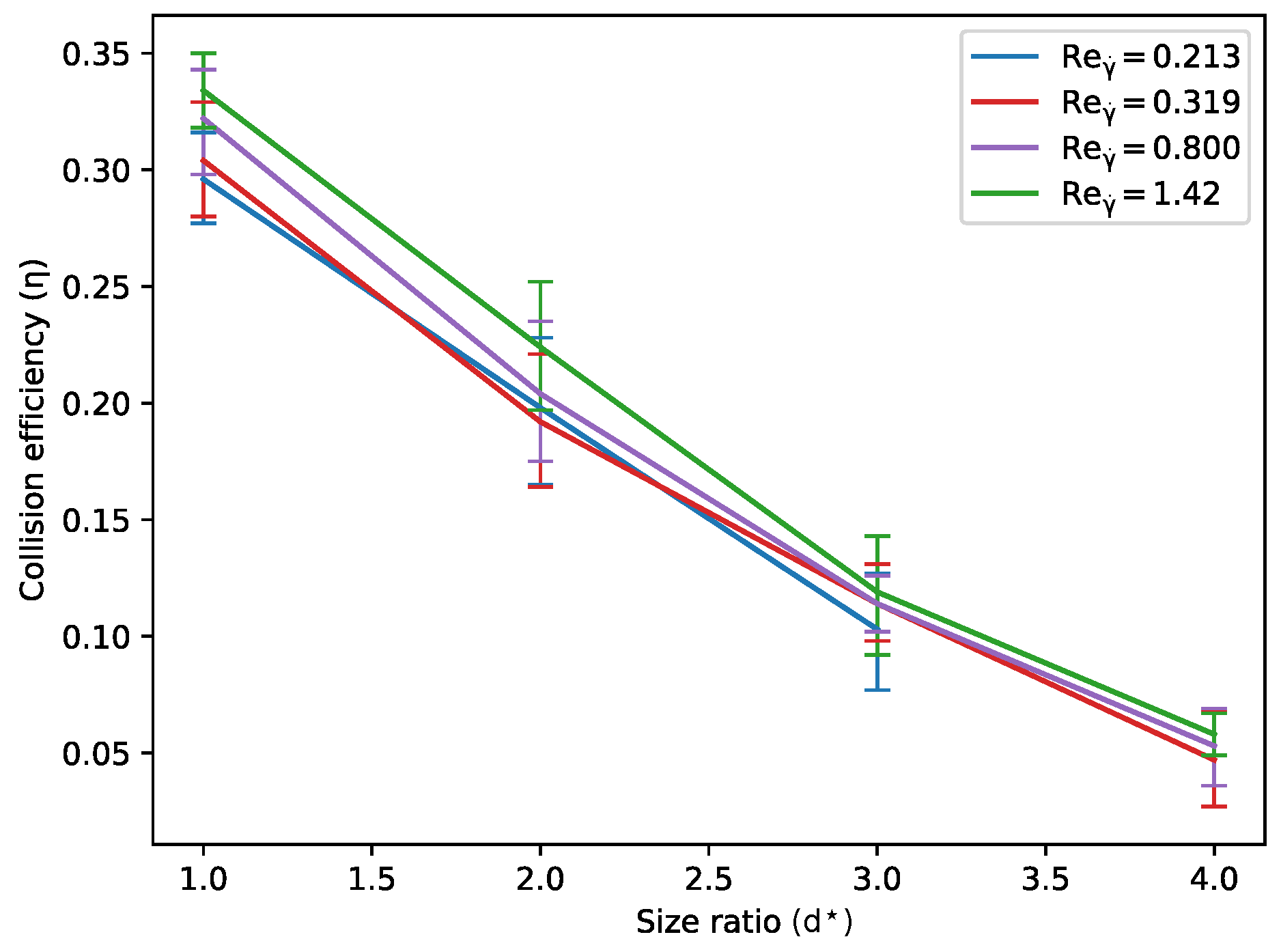
3.1.2. Impact of Particle Size Ratio

The change of the cross-section with the particle size ratio $d^{☆}$ is presented in Figure 3 for three values of the Reynolds number. The results show that in all cases the cross-section shrinks with increasing size ratio. This is because smaller particles have a shorter range of flow disturbance compared to bigger ones. Hence, they tend to better follow the streamlines in the flow which are affected by the disturbance of the bigger particle. For large particle size ratios, the bigger particle is almost not deviated at all, while the smaller one gets deviated significantly, which in the end leads to more avoidance.

In the range of Reynolds numbers investigated here, there is only one exception to this rule, which is for ${\mathrm{Re}}_{\dot{\gamma }}=1.42$, in Figure 3d, the “U-turn” avoidance is actually greater for particle size ratio of 1 than for higher size ratios. This is due to the convention that was chosen, namely to define the Reynolds number using the bigger particle diameter. Thus, when changing the size ratio from 2 to 1, the Reynolds number for the smaller particle gets bigger than 1, which inverts the trend of the “U-turn” avoidance since this avoidance is enhanced by both increasing size ratio and increasing Reynolds number. Unsurprisingly, the balance between both effects changes around a value of 1 of the Reynolds number.

3.1.3. Binary Collision Efficiency

Table 1. Collision efficiency for various combinations of shear Reynolds numbers and particle size ratios.

	${\mathbf{Re}}_{\dot{\mathit{\gamma }}}$
${\mathit{d}}^{☆}$	0.028	0.071	0.213	0.319	0.800	1.42
1	${0.290}_{-\phantom{+}0.041}^{+0.041}$	${0.293}_{-\phantom{+}0.021}^{+0.022}$	${0.296}_{-\phantom{+}0.019}^{+0.020}$	${0.304}_{-\phantom{+}0.024}^{+0.025}$	${0.322}_{-\phantom{+}0.024}^{+0.021}$	${0.334}_{-\phantom{+}0.016}^{+0.016}$
2			${0.198}_{-\phantom{+}0.033}^{+0.030}$	${0.192}_{-\phantom{+}0.028}^{+0.029}$	${0.204}_{-\phantom{+}0.029}^{+0.031}$	${0.224}_{-\phantom{+}0.027}^{+0.028}$
3			${0.103}_{-\phantom{+}0.026}^{+0.024}$	${0.114}_{-\phantom{+}0.016}^{+0.017}$	${0.114}_{-\phantom{+}0.012}^{+0.012}$	${0.119}_{-\phantom{+}0.027}^{+0.024}$
4				${0.047}_{-\phantom{+}0.020}^{+0.021}$	${0.053}_{-\phantom{+}0.017}^{+0.016}$	${0.058}_{-\phantom{+}0.009}^{+0.009}$

collects calculated collision efficiencies for various Reynolds numbers as well as various size ratios between the two interacting particles. The main value indicated in each cell of the table is the weighted efficiency, in which the surface area of triangles is weighted by the number of their vertices corresponding to collisions. In this way, the collision efficiency is thus derived from Equation (2), in which the collision cross-section is estimated as the total surface area of triangles, weighted by 1, $2/3$, $1/3$ or 0 in case they have 3, 2, 1 or 0 vertices corresponding to collisions. The error estimation, then, is obtained from calculating collision efficiencies from the upper and lower bounds of the cross-section area. The upper bound is obtained by attributing the weight 1 to all triangles with at least one collision vertex (triangles with all shades of orange from Figure 2), while the lower bound results from only counting triangles with three collision vertices (only dark orange region in Figure 2).

The change of the cross sections with the Reynold number shows that the interaction dynamics are significantly altered by the finite Reynolds number hydrodynamics. Some phenomena, like the avoidance region for small initial relative distance in direction of the shear, $\mathsf{\Delta }{z}_p^0$, reflect finite Reynolds number effects and are not observable under Stokes conditions. However, although cross sections vary with Reynolds number, when converted into statistical data the resulting collision efficiency barely varies over a quite large range of Reynolds numbers. Finite Reynolds number effects appear to cancel out. This means that fewer “pass by” avoidances resulting in slightly larger disc shape are compensated by increasing “U-turn” resulting in significant shift of the cut at the bottom of the disc (see Figure 3). The overall cross-section area decreases with the Reynolds number, but it also moves up, i.e., in the direction of the shear, so that it reaches areas corresponding to higher particle flux $\dot{\gamma }\mathsf{\Delta }{z}_p^0$, which compensates for the smaller area. In the end, despite a perceivable change in the cross sections, the Reynolds number has very little impact on the collision efficiency over a broad range of Reynolds numbers. This is illustrated in Table 1, where it can be seen that the variations of the efficiency with Reynolds number remain of the same order of magnitude as the accuracy of the calculation. The latter depends on the number of simulation points that were used to draw the cross-section.

For the sake of completeness, although the collision efficiency shows only little variations over a wide range of particulate Reynolds numbers for a monodisperse particle population, a linear fit is plotted in Figure 4. It was obtained from a generalized least square regression using the upper and lower bounds given in Table 1 for variance estimation. This procedure yields

$$\eta \left({\mathrm{Re}}_{\dot{\gamma }}\right)\approx 0.292+0.031{\mathrm{Re}}_{\dot{\gamma }}$$

(8)

On the other hand, the particle size ratio has a strong influence on the collision efficiency as illustrated in Figure 5. Table 1 shows a substantial drop of the collision efficiency when particles have different sizes, with a factor of 7 between a diameter ratio of 1 and 4. It is noteworthy that the collision efficiency drop with size ratio presented here is steeper than the power law given by [11] who used SD which only applies to very low Reynolds numbers. However it is clear that for Reynolds numbers that are not infinitely small, even for values down to $0.028$, non-linear effects in the flow play a significant role in particle interaction dynamics since the “U-turn” avoidance mechanism induced by flow recirculation loops around particles decreases the collision cross-section by a significant amount. Such recirculations scale with the flow dynamics at the particle size, not with the particle size ratio. As a result, the horizontal bottom line of the collision surface in in Figure 3 hardly moves when the size ratio varies. In this way, a piece of the collision cross-section is removed that gets bigger relative to the cross-section area that decreases with size ratio. As a conclusion, although collision efficiency does not quantitatively vary with Reynolds number, non-linearities in the flow have a strong impact on aggregation efficiency that cannot be captured with Stokesian Dynamics.

3.2. Aggregation Kinetics in a Bubbly Flow

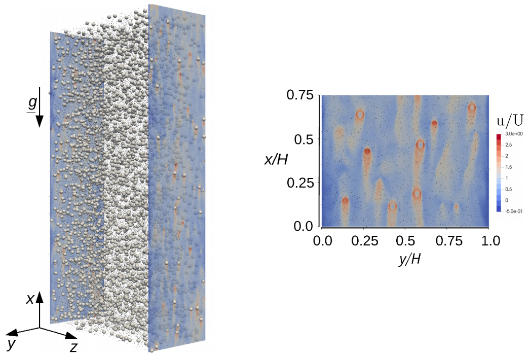
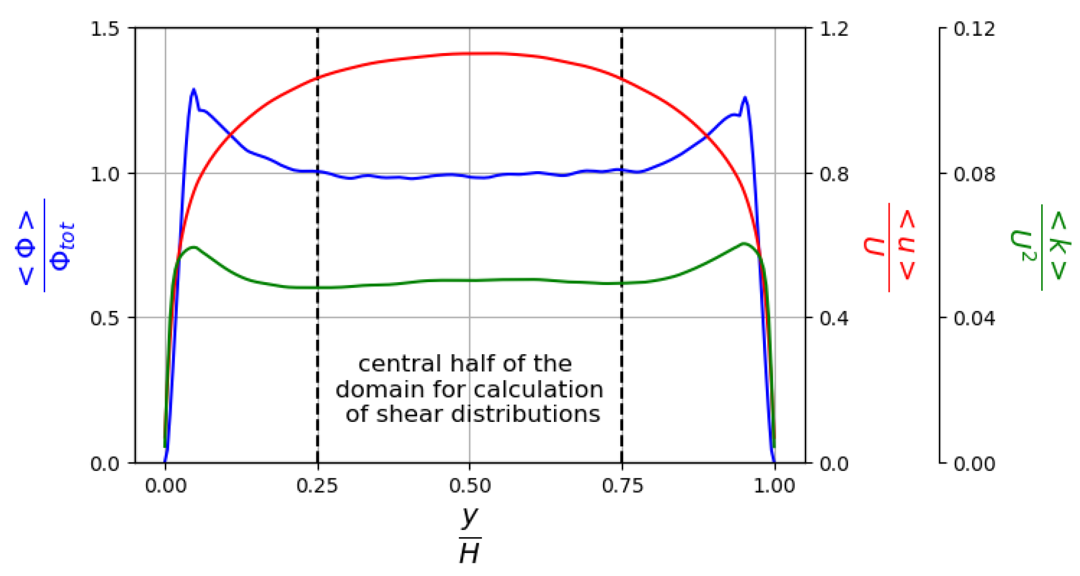
3.2.1. Channel Configuration

The configuration discussed in the following builds upon the case SmMany of [16] featuring an upward bubble-laden turbulent channel flow. Here, it was repeated and supplemented with the additional point particles. In contrast to that reference the simulation was performed with the IBM of [26]. This configuration was selected because experience and reference data were available from the earlier work, and–most of all–the physical configuration is suitable for the given purpose. The simulation itself was conducted in non-dimensional units. For the convenience of the reader, in

Table 2. Physical and numerical parameters of the channel flow simulation.

	Quantity	Symbol	Value
Liquid steel properties
	Fluid density	${\rho }_f$	$=7800$ [${\mathrm{kg}/\mathrm{m}}^3$]
	Kinematic viscosity	${\nu }_f$	$=7.1\times {10}^{-7}$ [${\mathrm{m}}^2/\mathrm{s}$]
	Surface tension	${\sigma }_f$	$=1.4$ [${\mathrm{kg}/\mathrm{s}}^2$]
	Channel width	H	$=0.025$ [m]
	Upward bulk velocity	U	$=0.15$ [m/s]
Argon properties
	Bubble density	${\rho }_b$	$=7.8$ [${\mathrm{kg}/\mathrm{m}}^3$]
	Bubble diameter	$D_b$	$=1.3\times {10}^{-3}$ [m]
	Bubble gas fraction	${\mathsf{\Phi }}_{tot}$	$=2.14\%$
Inclusion properties
	Particle density	${\rho }_p$	$=3950$ [${\mathrm{kg}/\mathrm{m}}^3$]
	Particle diameter	$D_p$	$=1.3\times {10}^{-5}$ [m]
Numerical parameters
	Domain size	[$L_x\times L_y\times L_z$]	= [$4.4H\times H\times 2.2H$]
	Number of cells	[$N_x\times N_y\times N_z$]	= [$1024\times 232\times 512$]
	Time step	$\mathsf{\Delta }t$	$=3.17\times {10}^{-5}\left[\mathrm{s}\right]$
	Number of bubbles	$N_b$	$=2880$
	Number of particles	$N_p$	$\approx 2.5\times {10}^6$ (initial)

the non-dimensional physical parameters are converted to the situation where the fluid is liquid steel with, e.g., argon bubbles being injected. It can be deduced that the total volume simulated is $76.1$ cm${}^3$ comprising gas bubbles and steel, and the volume of liquid steel alone is $74.5$ cm${}^3$. In an application the value of ${\rho }_b$ depends on the type of gas, the hydrostatic pressure of the liquid column, and the surface tension. It is taken to be 1/1000 of the liquid density here for convenience. The influence of this value on the result is negligible, as long as the ratio is two to three orders of magnitude. The number of particles reflects the inclusion density typically found in a gas-stirred ladle, with the value $n=2.4\times {10}^{10}$ inclusions/m${}^3$ used here. Table 2 also contains the numerical parameters, like the number of grid points and the time step which amounts to a CFL number of about 0.8.

Particle-particle collisions were disregarded in this simulation. Particle-wall collisions were accounted for by a reflection of the particle at the wall. Particle-bubble collisions were detected, and the particles removed when hitting the bubble surface. This mimics the attachment of particles to the bubbles, but in the present simulation only led to a very small decay of the total particle loading over the duration simulated. The rate is about $0.5$% of the total amount of particles per bulk time unit $H/U$.

Having developed the analysis on the scale of the inclusions, this knowledge was transferred to the length scale of a bubble swarm in a flotation process. To this end, the turbulent three-phase channel flow just described was simulated with the physical conditions assembled in Table 2. Since the results in Section 3.1.3 show that aggregation between particles of the same size is prevalent, a monodisperse particle population was investigated. The particle size of 13 $\mathsf{\mu }$m was chosen as a representative characteristic diameter for small metallurgical inclusions. Due to their density ratio of ${\rho }_p/{\rho }_f=0.506$ the inclusion particles have a rise velocity of $u_{p,\infty }=3.5\times {10}^{-5}$ m/s in this case.

Bubble-laden flows, as they occur in flotation processes of liquid metal in a ladle, are agitated by the bubble-generated turbulence, which typically is much stronger than any shear-generated turbulence, except very close to the walls. For the present flow this was demonstrated in [29] (Figure 5 of this reference). This impacts on the characterization of the particle-fluid interaction. In contrast to the shear-based Stokes number ${\mathrm{St}}_{\dot{\gamma }}$ used above at the particle scale, the bubbly flow considered here requires a different characterization. While in the general definition $\mathrm{St}={\tau }_p/{\tau }_f$ the particle time scale ${\tau }_p=\left({\rho }_p{D}_p^2\right)/\left(18{\rho }_f{\nu }_f\right)$ still applies, the characteristic fluid time scale ${\tau }_f$ is different. Ref. [29] demonstrated that bubble-induced turbulence is appropriately characterized by the length scale $L_f=D_b$ and the velocity scale $U_f=U_r$, with $U_r$ the characteristic relative bubble velocity. This yields the time scale ${\tau }_{f,b}=D_b/U_r$ for a bubble-driven flow, resulting in the Stokes number ${\mathrm{St}}_{p,b}={\tau }_p/{\tau }_{f,b}$. A detailed discussion of the intricacies of defining a relative velocity for geometrically resolved bubbles is provided in [16], together with a proposal for its evaluation. In this reference the relative bubble velocity was evaluated for the flow considered here as the difference between the mean bubble velocity and the mean fluid velocity, which is a function of the wall-normal position. The results show that the relative bubble velocity in this flow is close to uniform all over the domain. The value in the center of the flow is retained here for the definition of a global reference value and $U_r$ set to $0.85U$ according to [16]. This yields ${\mathrm{St}}_{p,b}=6.6\times {10}^{-4}$, which is extremely small. The particles, hence, follow the fluid extremely well. This addresses the particle-turbulence interaction.

It should not be forgotten, though, that the particles experience buoyancy and, thus, move upwards with respect to the liquid. In the present case this sedimentation velocity (although the inclusions move upwards) is $U_{\mathrm{sed}}=6.4\times {10}^{-5}$ m/s, which is extremely small. From a conceptual point of view, it is advantageous to work with uniform particle properties. In this case, sedimentation does not generate collisions between particles, as these all move with the same small velocity in stagnant fluid. Hence, all particle collisions detected in the DNS are due to turbulence. This allows immediate separation of the effects. Other concepts may, of course, be implemented.

3.2.2. Turbulent Liquid Steel and Argon Flow

For a first impression of the three-phase flow a snapshot is shown in Figure 6, with bubbles displayed to scale and particles enlarged by a factor of 10. Two contour plots are presented in planes perpendicular to the walls showing the instantaneous streamwise velocity component. The two parallel vertical walls are located perpendicular to the $y-$coordinate at a distance of H but were removed from the plot not to obstruct the view. Between these walls the bubble swarm and the inclusions rise in an upward-directed background flow. An imposed volume force $f_x$, which is constant in space and adjusted in each time step, yields the desired bulk velocity U, based on the flow rate of fluid and bubbles, such that the bulk Reynolds number is $\mathrm{Re}=UH/{\nu }_f=5263$. At the walls, a no-slip condition for the fluid velocity was applied. In the streamwise and spanwise direction the flow is periodic.

The statistical analysis of collision rates in the flow is best done with large-scale spatial homogeneity of the statistical properties. Figure 7 shows mean velocity, mean gas fraction and turbulent kinetic energy of the three-phase flow, obtained from averaging in wall-parallel planes, i.e., in x and z, as well as in time, once the statistically steady state established. It is obvious that the bubble volume fraction is constant over the interval $y/H=0.25\dots 0.75$. The same holds for the turbulent kinetic energy k, thus backing the dominance of bubble-induced turbulence stated above. This fact is even more backed by the analogous behavior of both curves beyond this interval. The mean streamwise velocity exhibits a small variation over this range in y. However, it only results in a slightly smaller or larger vertical transport of fluid, bubbles and particles with negligible mean shear being induced, so that homogeneity of the quantities considered later is not affected. According to these observations, simulation data in the center region $y/H=0.25\dots 0.75$ were used in the analysis. Furthermore, at a later stage this extension in y was checked to be appropriate by choosing different $y-$extensions of the extracted center region. The conditions of these data, hence, should correspond fairly well to the interior of a liquid metal flotation process with uniform bubble size.

After the statistically stationary state of the DNS was reached data were stored for post-processing. This was done, simultaneously, for the entire three-dimensional velocity fields with all velocity components and pressure, for the instantaneous bubble positions and velocities, as well as the instantaneous particle positions and velocities. Together with the fluid velocity data the shear rate

$$\dot{\gamma }=\sqrt{2{\left(d_{ij}\right)}^2}with{d}_{ij}=\frac{1}{2}\left(\frac{\partial u_i}{\partial x_j}+\frac{\partial u_j}{\partial x_i}\right)$$

(9)

was determined as well. This was done employing the staggered grid used for the simulation and yielded the shear rate on a cell-centered grid. The simulated volume and the number of bubbles and particles inside the domain are all large enough to contain statistically representative data in a single snapshot.

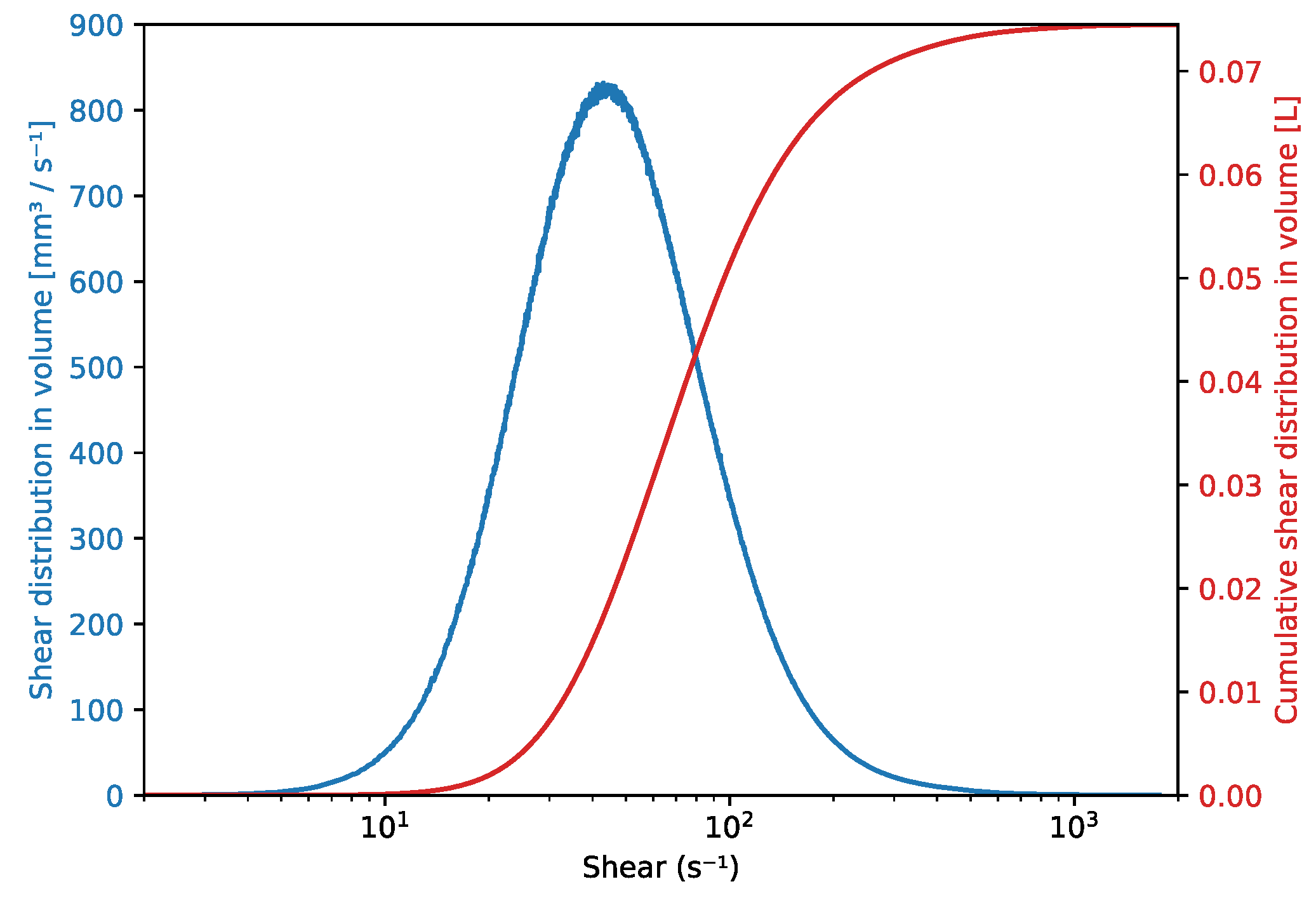
3.2.3. Determination of Collision Frequency

The definition of collision efficiency in Equation (2) uses the collision kernel of Smoluchowski [21]. This provides an analytical solution to collision in plane shear by neglecting hydrodynamic interactions between particles. In a turbulent flow, local velocity gradients do not only correspond to plane shear flow but exhibit more complex structure. This led Saffman and Turner [8] to develop a similar solution driven by local turbulence properties but still without considering hydrodynamic interactions. When expressing their collision kernel as a function of characteristic shear rate associated with turbulence dissipation, their solution is qualitatively and quantitatively equivalent to the one of Smoluchowski [21].

$${\beta }_{ij}^{\mathrm{Smol}.}=\frac{1}{6}\dot{\gamma }{\left(d_{pi}+d_{pj}\right)}^3\approx {\beta }_{ij}^{\mathrm{S}.＆\mathrm{T}.}=\sqrt{\frac{\pi }{120}}\underset{{\displaystyle \dot{\gamma }}}{\underbrace{\sqrt{\epsilon /\nu }}}{\left(d_{pi}+d_{pj}\right)}^3$$

(10)

Indeed, both solutions are driven by local velocity gradients and the results obtained with them are very close, with a relative difference in efficiency less than 3%. Because of these similarities, determining the collision efficiency in a turbulent flow based on the mesoscopic situation of plane shear seems to be appropriate.

The aggregation frequency $f_{ij}$ is the number of aggregation events per unit time in the liquid volume ${\mathcal{V}}_{\mathrm{liq}}$. In a turbulent flow, this quantity can be expressed as a function of the aforementioned collision efficiency ${\eta }_{ij}$ and the collision kernel from [8] as

$$f_{ij}={\int }_{{\displaystyle {\mathcal{V}}_{\mathrm{liq}}}}{\eta }_{ij}\left(\dot{\gamma }\right)\sqrt{\frac{\pi }{120}}\dot{\gamma }{\left(d_{pi}+d_{pj}\right)}^3{n}_i{n}_j\mathrm{d}\mathcal{V}$$

(11)

where $n_i$ is the number density function of particles of class i. The number of particles of this class, $N_i$, in a given volume $\mathcal{V}$ can then be expressed by integration over this volume

$$N_i\left(\mathcal{V}\right)={\int }_{\mathcal{V}}{n}_i\mathrm{d}\mathcal{V}$$

(12)

Since the effective collision kernel introduced in Equation (2), is a function of the shear rate, Equation (11) would be more practical in the form of an integral over the shear rate, instead of the volume, i.e.,

$$f_{ij}={\int }_0^{\infty }{\eta }_{ij}\left(\dot{\gamma }\right)\sqrt{\frac{\pi }{120}}\dot{\gamma }{\left(d_{pi}+d_{pj}\right)}^3{n}_i{n}_j\frac{\partial \mathcal{V}}{\partial \dot{\gamma }}\mathrm{d}\dot{\gamma }$$

(13)

This change of variables requires the volume cumulative distribution function according to shear rate

$$\mathcal{V}\left(\underset{\tilde{}}{\dot{\gamma }}\right)=\underset{{\displaystyle {\mathcal{V}}_{\mathrm{liq}}}}{\int \int \int }\mathcal{H}\left(\underset{\tilde{}}{\dot{\gamma }}-\dot{\gamma }\left(\mathbf{x}\right)\right)\mathrm{d}{x}^3$$

(14)

where $\mathcal{H}$ is the Heaviside step function, so that function $\mathcal{V}$ is the cumulative distribution of shear in volume. The number density of particles can then also be expressed as a function of the shear rate, reading

$$n_i=\frac{\partial N_i}{\partial \mathcal{V}}=\frac{\partial N_i}{\partial \dot{\gamma }}{\left(\frac{\partial \mathcal{V}}{\partial \dot{\gamma }}\right)}^{-1}$$

(15)

Finally, Equations (14) and (15) can be injected into Equation (13) to yield a shear-based expression of the aggregation frequency

$$f_{ij}=\sqrt{\frac{\pi }{120}}{\left(d_{pi}+d_{pj}\right)}^3{\int }_0^{\infty }{\eta }_{ij}\left(\dot{\gamma }\right)\frac{\partial N_{i\phantom{j}}}{\partial \dot{\gamma }}\frac{\partial N_j}{\partial \dot{\gamma }}{\left(\frac{\partial \mathcal{V}}{\partial \dot{\gamma }}\right)}^{-1}\dot{\gamma }\mathrm{d}\dot{\gamma }$$

(16)

This new expression now depends on two shear distributions: the shear distribution in the volume $\left(\frac{\partial \mathcal{V}}{\partial \dot{\gamma }}\right)$ and the shear distribution among the particles $\left(\frac{\partial N_i}{\partial \dot{\gamma }}\right)$. These two statistical quantities can be extracted from DNS simulations of the particle-laden bubbly flow, and this was done in the present study to provide a first application.

3.2.4. Results for Collision Rates

In the three-phase flow considered here, particles are monodisperse, so Equation (16) boils down to

$$f=\sqrt{\frac{\pi }{15}}{d}_p^3{\int }_0^{\infty }\eta \left({\mathrm{Re}}_{\dot{\gamma }}\right){\left(\frac{\partial N}{\partial \dot{\gamma }}\right)}^2{\left(\frac{\partial \mathcal{V}}{\partial \dot{\gamma }}\right)}^{-1}\dot{\gamma }\mathrm{d}\dot{\gamma }$$

(17)

Since particles are not necessarily distributed uniformly in space and over all shear rates, the shear rate distribution experienced by the particles was calculated from the DNS by calculating the local shear rate at each particle position from the velocity field using Equation (9). The shear rate distribution among particles is defined as the derivative of a cumulative function in the same way as done for volume in Equation (14), so that

$$N\left(\underset{\tilde{}}{\dot{\gamma }}\right)=\sum _p\mathcal{H}\left(\underset{\tilde{}}{\dot{\gamma }}-\dot{\gamma }\left({\mathbf{x}}_p\right)\right)$$

(18)

where ${\mathbf{x}}_p$ is particle position, and $\dot{\gamma }\left({\mathbf{x}}_p\right)$ is thus the value of the shear rate in the cell where the particle is located.

The distribution of the shear rate with respect to the liquid volume and with respect to the particle positions that appear in Equation (17) were obtained from the three-phase DNS. They are displayed in Figure 8 and Figure 9, respectively. These two distributions superimpose perfectly, which means that inclusions do not segregate in regions with specific shear such as inside or outside of bubble wakes. This does not come as a surprise due to their very low Stokes number ${\mathrm{St}}_{p,b}$. It confirms that although direct interception of inclusions by bubbles happens, it only impacts the total number inclusions in the volume, but has no significant impact on their repartition. Inclusion capture at bubble surfaces does not induce a depletion of their concentration in bubble wakes. Figure 9 also shows that the shear rate seen by most inclusions (peak of the distribution) is around 40 s${}^{-1}$ while the median shear rate undergone by inclusions is about 70 s${}^{-1}$, and the average (not directly readable form the figure) is about 100 s${}^{-1}$.

Local shear is the only driving force in this study. Equation (17) shows that the contribution due to each shear rate is weighted by the shear rate value and the corresponding collision efficiency. Figure 10 shows the contribution of all shear rates to the overall collision rate in distribution form ($\partial f/\partial \dot{\gamma }$) and in cumulative form (partial integration for shears between 0 and $\dot{\gamma }$). The distribution peaks at $\dot{\gamma }\approx 60{\mathrm{s}}^{-1}$, and the median shear rate in terms of contribution to the total collision frequency is 200 s${}^{-1}$. Figure 10 also shows that all shear rates above 20 s${}^{-1}$ up to 1000 s${}^{-1}$ contribute to aggregation, i.e., in the Reynolds range up to $0.235$. Since $\epsilon =\nu {\dot{\gamma }}^2$, this range of shear rates from 20 s${}^{-1}$ to 1000 s${}^{-1}$ is equivalent to a range of stirring power dissipated in the steel bath from $0.3$ W to 710 W per ton of liquid steel which are typical values encountered in ladle treatment [1].

Finally, numerically integrating Equation (17) with distributions from the present DNS data yields a quantitative collision frequency of $1.24\times {10}^3$ s${}^{-1}$ (collision per seconds) in the considered volume of liquid steel of 74.5 cm${}^3$. It corresponds to $16.6\times {10}^6$ s${}^{-1}$m${}^{-3}$ (collisions per second per cubic meter of liquid steel) which, in turn, gives a characteristic time of 860 s between two collisions undergone by the same inclusion, here with diameter 13 $\mathsf{\mu }$m.

Since collisions between particles of the same size dominate, as demonstrated further above, and since the collision frequency increases quickly with inclusion size, the long characteristic time between collisions of inclusions of small size is the bottleneck of the whole aggregation process and is responsible for the long processing time of steel ladles.

4. Conclusions

A multiscale approach was developed to simulate inclusion collision behavior and aggregation kinetics in liquid steel agitated by bubble swarm. It couples fully resolved flow simulations at inclusion scale (a few tens of microns) and at bubble swarm scale (a few tens of centimeters) through statistical models. Characteristic scales of the process are extracted by post-processing the simulations, such as time between collisions in an agitated bubbly region in the ladle.

Hydrodynamic interactions have a significant impact on particle collision dynamics at low but finite Reynolds numbers, conditions prevailing for small non-metallic inclusions. Such effects are accounted for in the collision efficiency derived from fully resolved inclusion interaction dynamics. The coupling with bubble swarm DNS shows how this efficiency can be used to upscale this information to a bubbly flow with very many particles. Inclusions are low inertia particles that closely follow streamlines in the flow. The fact that their Stokes number is not exactly zero allows some of them to be captured by direct interception by bubbles, but apart from that they show no preferential distribution between regions of different shears and remain homogeneously distributed in the liquid metal phase.

The most significant feature of the collision efficiency at moderately low Reynolds number is its low value: for particles of the same size, it is approximately 0.3 which is markedly smaller than one. Due to the lack of fully resolved collision studies, many state-of-the-art process simulations rely on collision kernels that do not account for short-range hydrodynamic interactions, such as the closures of Smoluchowski [21] and Saffman and Turner [8]. However, accounting for such short-range interactions divides by three the probability of collision between particles of the same size ($\eta \approx 0.3$ for $d^{☆}=1$) which significantly slows down aggregation kinetics. The collision efficiency also drops very steeply when increasing the particle size ratio. As a result, aggregation kinetics are ruled by aggregation between particles within the same size range. This, in turn, has important implications for accurately capturing the kinetics of processes with broad particle size distributions, especially in population balance simulations that lack reliable interactions models in which collisions with bigger particles play a non-negligible role on aggregation of small particles.

References

1. Zhang, L.; Thomas, B.G. State of the art in evaluation and control of steel cleanliness. ISIJ Int. 2003, 43, 271–291. [Google Scholar] [CrossRef] [Green Version]
2. Zhang, L.; Li, Y.; Ren, Y. Fundamentals of Non-Metallic Inclusions in Steel: Part II. Evaluation Method of Inclusions and Thermodynamics of Steel Deoxidation. Iron Steel 2013, 12, 1–8. [Google Scholar]
3. Cournil, M.; Gruy, F.; Gardin, P.; Saint-Raymond, H. Modelling of solid particle aggregation dynamics in non-wetting liquid medium. Chem. Eng. Process. Process. Intensif. 2006, 45, 586–597. [Google Scholar] [CrossRef]
4. Bellot, J.P.; De Felice, V.; Dussoubs, B.; Jardy, A.; Hans, S. Coupling of a CFD and a PBE calculations to simulate the behavior of an inclusion population in a gas-stirred ladle. Metall. Mater. Trans. B 2014, 45, 13–21. [Google Scholar] [CrossRef]
5. De Felice, V.; Daoud, I.L.A.; Dussoubs, B.; Jardy, A.; Bellot, J.-P. Numerical modelling of inclusion behaviour in a gas-stirred ladle. ISIJ Int. 2012, 52, 1274–1281. [Google Scholar] [CrossRef] [Green Version]
6. Lou, W.; Zhu, M. Numerical Simulations of Inclusion Behavior in Gas-Stirred Ladles. Metall. Mater. Trans. B 2013, 45, 762–782. [Google Scholar] [CrossRef]
7. Bellot, J.-P.; Kroll-Rabotin, J.-S.; Gisselbrecht, M.; Joishi, M.; Saxena, A.; Sanders, R.S.; Jardy, A. Toward better control of inclusion cleanliness in a gas stirred ladle using multiscale numerical modeling. Materials 2018, 11, 1179. [Google Scholar] [CrossRef] [Green Version]
8. Saffman, P.G.F.; Turner, J.S. On the collision of drops in turbulent clouds. J. Fluid Mech. 1956, 1, 16–30. [Google Scholar] [CrossRef] [Green Version]
9. Higashitani, K.; Ogawa, R.; Hosokawa, G.; Matsuno, Y. Kinetic theory of shear coagulation for particles in a viscous fluid. J. Chem. Eng. Jpn. 1982, 15, 299–304. [Google Scholar] [CrossRef] [Green Version]
10. Van de Ven, T.G.M.; Mason, S.G. The microrheology of colloidal dispersions VII. Orthokinetic doublet formation of spheres. Colloid Polym. Sci. 1977, 255, 46–479. [Google Scholar] [CrossRef]
11. Bülow, F.; Nirschl, H.; Dörfler, W. Simulating orthokinetic heterocoagulation and cluster growth in destabilizing suspensions. Particuology 2017, 31, 117–128. [Google Scholar] [CrossRef]
12. Vanni, M.; Baldi, G. Coagulation efficiency of colloidal particles in shear flow. Adv. Colloid Interface Sci. 2002, 97, 151–177. [Google Scholar] [CrossRef]
13. Frungieri, G.; Vanni, M. Dynamics of a shear-induced aggregation process by a combined Monte Carlo-Stokesian Dynamics approach. In Proceedings of the 9th International Conference on Multiphase Flow, Florence, Italy, 22–27 May 2016. [Google Scholar]
14. Frungieri, G.; Vanni, M. Shear-induced aggregation of colloidal particles: A comparison between two different approaches to the modelling of colloidal interactions. Can. J. Chem. Eng. 2017, 95, 1768–1780. [Google Scholar] [CrossRef] [Green Version]
15. Haddadi, H.; Morris, J.F. Topology of pair-sphere trajectories in finite inertia suspension shear flow and its effects on microstructure and rheology. Phys. Fluids 2015, 14, 043302. [Google Scholar] [CrossRef]
16. Santarelli, C.; Fröhlich, J. Direct Numerical Simulations of spherical bubbles in vertical turbulent channel flow. Influence of bubble size and bidispersity. Int. J. Multiph. Flow 2016, 81, 27–45. [Google Scholar] [CrossRef]
17. Gisselbrecht, M.; Kroll-Rabotin, J.-S.; Bellot, J.-P. Aggregation kernel of globular inclusions in local shear flow: application to aggregation in a gas-stirred ladle. Metall. Res. Technol. 2019, 116, 512. [Google Scholar] [CrossRef]
18. Eggels, J.G.M.; Somers, J.A. Numerical simulation of free convective flow using the lattice-Boltzmann scheme. Int. J. Heat Fluid Flow 1995, 16, 357–364. [Google Scholar] [CrossRef]
19. Niu, X.D.; Shu, C.; Chew, Y.T.; Peng, Y. A momentum exchange-based immersed boundary-lattice Boltzmann method for simulating incompressible viscous flows. Phys. Lett. A 2006, 354, 173–182. [Google Scholar] [CrossRef]
20. Gisselbrecht, M. Simulation des Interactions Hydrodynamiques Entre Inclusions Dans un méTal Liquide: éTablissement de Noyaux d’agrégation dans les Conditions Représentatives du Procédé de Flottation. Ph.D. Thesis, Université de Lorraine, Nancy, France, 2019. (In French). [Google Scholar]
21. Smoluchowski, M.V. Drei Vorträge über Diffusion, Brownsche Bewegung und Koagulation von Kolloidteilchen. Z. Fur Phys. 1916, 17, 557–585. (In German) [Google Scholar]
22. Aland, S.; Schwarz, S.; Fröhlich, J.; Voigt, A. Modeling and numerical approximations for bubbles in liquid metal. Eur. Phys. J. Spec. Top. 2013, 220, 185–194. [Google Scholar] [CrossRef]
23. Heitkam, S.; Drenckhan, W.; Fröhlich, J. Packing Spheres Tightly: Influence of Mechanical Stability on Close-Packed Sphere Structures. Phys. Rev. Lett. 2012, 108, 148302. [Google Scholar] [CrossRef] [PubMed]
24. Schiller, L.; Naumann, A. A Drag Coefficient Correlation. Z. Des Vereins Dtsch. Ingenieure 1935, 77, 318–320. (In German) [Google Scholar]
25. Kempe, T.; Fröhlich, J. An improved immersed boundary method with direct forcing for the simulation of particle laden flows. J. Comput. Phys. 2012, 9, 3663–3684. [Google Scholar] [CrossRef]
26. Tschisgale, S.; Kempe, T.; Fröhlich, J. A general implicit direct forcing immersed boundary method for rigid particles. Comput. Fluids 2018, 170, 285–298. [Google Scholar] [CrossRef]
27. Dormand, J.R.; Prince, P.J. A family of embedded Runge-Kutta formulae. J. Comput. Appl. Math. 1980, 6, 19–26. [Google Scholar] [CrossRef] [Green Version]
28. May, R.; Gruy, F.; Fröhlich, J. Impact of particle boundary conditions on the collision rates of inclusions around a single bubble rising in liquid metal. Proc. Appl. Math. Mech. 2018, 18, e201800029. [Google Scholar] [CrossRef]
29. Ma, T.; Santarelli, C.; Ziegenhein, T.; Lucas, D.; Fröhlich, J. Direct numerical simulation–based Reynolds-averaged closure for bubble-induced turbulence. Phys. Rev. Fluids 2017, 2, 034301. [Google Scholar] [CrossRef]
Figure 1. Schematic of a gas-stirred ladle.
Metals 10 00517 g001
Figure 2. Simulation setup with visible subdivision algorithm to guide the cross-section calculation, the orange region on the right-hand side represents the effective cross-section, with the color intensity level corresponding to the number of nodes of each triangle leading to collision.
Metals 10 00517 g002
Figure 3. Contours of cross sections for binary collision between particles: (a) particles of the same size ( d = 1 ) at various Reynolds numbers, Re γ ˙ 0.028 , , 1.42 . (bd) collision surfaces at specific Reynolds numbers for various size ratios, d : Metals 10 00517 i0011, Metals 10 00517 i0022, Metals 10 00517 i0033, Metals 10 00517 i0044.
Metals 10 00517 g003
Figure 4. Collision efficiency for monodisperse particles as a function of Reynolds number: results from LBM simulations and linear fit from Equation (8).
Metals 10 00517 g004
Figure 5. Collision efficiency from LBM simulations as a function of particle size ratio.
Metals 10 00517 g005
Figure 6. Illustration of the three-phase channel flow simulation. Left: Computational domain and snapshot of the solution in perspective view with two contour plots of the instantaneous vertical velocity component u in wall-normal planes close to the periodic boundaries. Right: u in a zoom of a wall-normal plane at an arbitrary position z = const . With the IBM the fluid velocity is also computed inside the bubbles. The particles shown are those in a small slab of thickness 0.025 H in z. They are drawn larger than to scale to make them visible in the plot at all.
Metals 10 00517 g006
Figure 7. Gas fraction (in blue), mean streamwise velocity (in red) and turbulent kinetic energy (in green) as functions of the wall-normal coordinate in the DNS of the bubbly three-phase flow.
Metals 10 00517 g007
Figure 8. Shear rate distribution in volume: V / γ ˙ in blue and V ( γ ˙ ) from Equation (14) in red.
Metals 10 00517 g008
Figure 9. Shear rate distribution among particles: N / γ ˙ in blue and N ( γ ˙ ) from Equation (18) in red.
Metals 10 00517 g009
Figure 10. Contribution of shear rates to collision frequency.
Metals 10 00517 g010