Finite Strain Homogenization Using a Reduced Basis and Efficient Sampling


Efficient Methods for Mechanical Analysis, Institute of Applied Mechanics (CE), University of Stuttgart, 70569 Stuttgart, Germany
*
Author to whom correspondence should be addressed.
Math. Comput. Appl. 2019, 24(2), 56; https://doi.org/10.3390/mca24020056
Submission received: 31 March 2019
/
Revised: 24 May 2019
/
Accepted: 24 May 2019
/
Published: 27 May 2019
(This article belongs to the Special Issue Machine Learning, Low-Rank Approximations and Reduced Order Modeling in Computational Mechanics)
Abstract
:The computational homogenization of hyperelastic solids in the geometrically nonlinear context has yet to be treated with sufficient efficiency in order to allow for real-world applications in true multiscale settings. This problem is addressed by a problem-specific surrogate model founded on a reduced basis approximation of the deformation gradient on the microscale. The setup phase is based upon a snapshot POD on deformation gradient fluctuations, in contrast to the widespread displacement-based approach. In order to reduce the computational offline costs, the space of relevant macroscopic stretch tensors is sampled efficiently by employing the Hencky strain. Numerical results show speed-up factors in the order of 5–100 and significantly improved robustness while retaining good accuracy. An open-source demonstrator tool with 50 lines of code emphasizes the simplicity and efficiency of the method.
Keywords:
computational homogenization; large strain; finite deformation; geometric nonlinearity; reduced basis; reduced-order model; sampling; Hencky strainMSC:
74Q05; 74B20; 74S301. Introduction
1.1. Purpose
The description of solid mechanics under finite strains is of particular interest in both academia and industry. It allows for accurate descriptions of rotations and stretches under mild assumptions. Thus, many geometric effects can be captured. For instance, alignments and rearrangements of the respective structures may trigger pronounced stiffening or softening effects.
In such cases where rotations and deformations are not suitable for linearization, dissipative effects also play a notable role for many materials. Regardless of the kind of dissipation involved in a certain process, hyperelasticity usually persists to a certain extent. Therefore, it is worthwhile investigating this comparatively simple case at first, before introducing history dependence into the description. Prominent examples of materials that require a hyperelastic description at finite strains include carbon black-filled rubber [1] and amorphous glassy polymers [2], to name just two.
The main purpose of this work is the computationally efficient quasi-static homogenization of hyperelastic solids with full account for geometric nonlinearities. The employed methodology is twofold. First, a Reduced Basis (RB) model for the microscopic problem is established. The term Reduced Basis, used in this work, is not to be confused with the homonymous method introduced by Barrault, Maday, Nguyen, and Patera [3]. Once set up, it enables more efficient evaluations of the homogenized material response as compared to the Finite Element Method (FEM). Second, an efficient strategy for sampling of the space of macroscopic kinematic states is proposed. This renders the setup phase of the RB model more rational.
1.2. State of the Art
Efficiently determining the overall solid–mechanical properties of microstructures has been investigated for decades, and a large body of literature is available. Comprehensive review articles, such as [4] and [5], summarize the progress. Here, attention is restrained to few methods most similar or relevant to the present work.
The FE2 method [6] is theoretically capable of performing realistic two-scale simulations with arbitrary accuracy. Therefore, it serves as a reference method in the context of first-order homogenization based on the assumption of separated length scales. In the FE2, the evaluations of the unknown macroscopic constitutive law are approximated by microscopic FE simulations. However, this comes along with computational costs that quickly exceed the capabilities of common workstations, both at present and in the foreseeable future. Roughly speaking, the computational effort required on the microscale multiplies with that of the macroscale, hence the method’s name. It is thus worthwhile to develop order reduction methods for the microscopic problem.
A common approach within the field of computational homogenization (and well beyond) is to extract essential information from provided in silico data. To this end, schemes based on the Proper Orthogonal Decomposition (POD) compute correlations within snapshot data, [7]. Such methods include the R3M [8] and can be further enhanced by the use of, e.g., the EIM, as in [9]. Numerical comparisons of various schemes were conducted in [10,11]. To the best of the authors’ knowledge, all published POD-based methods addressing the finite strain hyperelastic problem choose to reduce the number of degrees of freedom (DOF) of the displacement field. This results in sometimes significant speed-ups. Another important feature is that they allow for reconstruction of the microscopic displacement fields. The application of the snapshot POD to gradients of the primal variables has been studied—e.g., for infinitesimal strain hyperelasticity [12] and fluid mechanics [13]—but does not appear to have been investigated for finite strain hyperelasticity yet.
Still, the solution of the reduced equations remains a complex task. It requires evaluations of material laws and numerical integration over the microstructure. Promising progress has been made in the field of efficient integration schemes, see for instance [14,15]. A main reason for the speed-up of these methods is the reduced number of function evaluations.
The highest speed-ups are achievable if the computational effort of the determination of effective microstructural responses can be fully decoupled from underlying microstructural discretizations. Such homogenization methods directly approximate the effective material law by means of a dedicated numerical scheme. Technically, this can be seen as the direct surrogation of unknown functions, e.g., of the effective free energy or stress. For instance, the Material Map [16] interpolates the coefficients of an assumed macroscopic material model. Another example is the NEXP method [17], where the effective stored energy density is approximated using a tensor product of one-dimensional splines. The authors treated the case of small strains by introducing the RNEXP method [12], where the effective stored energy is interpolated by a dedicated kernel scheme.
However, interpolatory and regressional methods suffer the inherent drawback of not providing any explicit information on the microscale. For instance, microscopic displacement or stress fields cannot be reconstructed from the solutions of macroscopic interpolation. Another important open question is how to provide the supporting data points for the interpolation in an efficient manner. The data at these points is usually provided by the solution of a full-order model (FOM) and come along with the corresponding numerical costs. Hence, the positions of data points in the parameter space should be chosen carefully, as unnecessary or redundant solutions of the FOM should be avoided. On the other hand, too sparsely seeded points might not capture the homogenized properties of the microstructure appropriately.
1.3. Main Contributions and Outline
The present work generalizes parts of the previous paper [12] to the finite strain regime. It aims at reducing the computational complexity for the determination of the homogenized microstructural response, which is parametrized by the macroscopic deformation gradient acting as a boundary condition. This is achieved by means of a Reduced Basis approximation of the microscopic deformation gradient. The basis is obtained with the aid of a POD of snapshots of fluctuation fields of the deformation gradient. Thus, the application of the RB model does not necessitate the computation of gradients of displacement fields, and even does not require the displacements to be available at all. In other words, microscopic displacement fields are completely avoided. However, they can be reconstructed from the RB approximation of the deformation gradient, uniquely up to rigid body motion.
Another key advantage is the sleek implementation of the method. A demonstration containing a minimum working example of the RB model with 50 lines of MATLAB/Octave code is provided [18].
As for the setup phase, the snapshot data is created by means of an efficient sampling procedure for the microscopic boundary condition. To this end, the set of macroscopic Hencky strains is identified as a suitable linear parameter space, within which the sampling sites are placed based upon physical interpretation. This allows for control of the resolution of certain key characteristics of the effective material response while keeping the total number of samples within bounds.
1.4. Notation
The set of real numbers and the subset of positive numbers greater than zero are denoted by and , respectively. Matrices are marked by two underlines and vectors by one underline, e.g., , . Vectors are assumed to be columns, and the dot product of two vectors of the same size is understood as the Euclidean scalar product, . First order and second order tensors in coordinate-free description are denoted by bold letters, e.g., A, a. No conclusion can be drawn on the order of a tensor based on its capitalization. Here, the underlying space is always the Euclidean space with its standard basis. First order and second order tensors can be represented as vectors and matrices, e.g., and , respectively. Norms of vectors and matrices respectively denote the Euclidean and the Frobenius norm. The norm of a tensor of second order equals the norm of its matrix representation for the chosen basis. Fourth order tensors are denoted by blackboard bold symbols other than , e.g., and . Components of tensors of order M are with respect to the Euclidean tensorial basis , e.g., , for second order tensors A, B and , for , . The following contractions are defined:
Let be the domain occupied by a physical body undergoing elastic deformations, and let be its initial configuration. Then, x and X describe the coordinates of material points within the current configuration and within the reference state , respectively. Their difference is the displacement , see Figure 1. The gradient of a vector field is defined as a right gradient and denoted by . The divergence of a second order tensor field is the vector field resulting from row-wise divergence. The boundaries of the respective configurations are denoted by and . The set of square-integrable Lebesgue functions on the reference domain is tagged .
The displacement gradient and the deformation gradient are related through , where I is the second order identity tensor in three dimensions. The determinant measures the relative volumetric change due to the present deformation.
Unimodular quantities, i.e., second order tensors with determinant ones, may be emphasized by a hat, e.g., . This multiplicative decomposition is sometimes attributed to Flory [19] and also goes by the name Dilatational-Deviatoric Multiplicative Split (DDMS).
In the two-scale context, overlined symbols represent quantities on the macroscopic scale, e.g., , , while symbols without overline correspond to their microscopic counterpart, e.g., A, a. Equivalently, macroscopic quantities are called global and microscopic ones are called local. The volume average of a general local field
is essential to the theory. The dependence of a microscopic quantity A on both the microscopic coordinates X and a macroscopic quantity is denoted by . In such a case, the components of the macroscopic quantity are called parameters of the microscopic function . The application of the volume averaging operator is abbreviated by . The case of a concatenated function is analogous, i.e. , regardless of the tensorial order of the image of the function f.
1.5. Material Models
In this work, hyperelastic materials are investigated. They are characterized by stored energy density functions . The first Piola–Kirchhoff stress
and the corresponding fourth-order stiffness tensor
characterize the material response.
Henceforth, for reasons of readability, the stored energy density function W will be spoken of as an energy, and the terms stored and density will not always be mentioned explicitly. In the infinitesimal strain framework, hyperelastic energies have been formulated to model deformation plasticity (e.g., [12,17,20]). Although these models are only valid for purely proportional loading conditions, they provide means to simulate highly nonlinear material behavior in certain scenarios comparably easily within the context of hyperelasticity. Note that genuine dissipative processes require additional state describing variables with corresponding evolution laws.
The proposed method is suitable for any type of hyperelastic constitutive law. As the modeling of complex material behavior is not the main focus of this study, the Neo–Hookean law
is used, with K the bulk modulus and G the shear modulus. The volumetric part of the energy is taken from [21]. Using the DDMS, a decoupled dependence on the volumetric and isochoric part of the deformation is assumed, which is a common way to model the distinct material behavior with respect to these two contributions, see e.g., [22].
1.6. Problem Setting of First Order Homogenization
Assuming stationarity and separability of scales, the following coupled and deformation-driven problems can be derived by means of asymptotic expansion of the displacement u and subsequent first order approximation. This procedure is carried out in [23] with much detail. Here, the technical process is omitted and only the resulting equations are stated.
1.6.1. Macroscopic Problem
Balance of linear momentum
where denote bulk forces, and balance of angular momentum
along with well-posed boundary conditions that constitute the macroscopic boundary value problem. This system of equations is closed by means of the hyperelasticity law, cf. (2),
Note that, in general, is a priori not available and is thus a purely formal relation. For reasons of readability, the dependence of any quantity on the macroscopic material coordinate is usually spared, e.g., , , or .
1.6.2. Microscopic Problem
The microscopic boundary value problem is given by the balance equations
and suitable boundary conditions, e.g., as discussed in [24]. In this work, periodic displacement fluctuation boundary conditions are employed. The microscopic displacements take the form
Therein, the macroscopic displacement is independent of microscopic quantities. The second term, , corresponds to a homogeneous deformation of the microstructure. The third term, , is a displacement fluctuation with the zero mean property . Hence, the deformation gradient reads
where the fluctuation part , has the zero mean property
Thus, the volume average of the local deformation gradient equals its macroscopic counterpart,
This motivates the identification of as the boundary condition to the microscopic problem (8). As for the material response, the following relationships can be deduced:
Equations (13) and (15) are called kinematic and static coupling relations, respectively. The inequality (16) generally holds for heterogeneous microstructures, even in the most simple case of infinitesimal strains and linear elasticity. More precisely, the volume average overestimates the effective stiffness in the spectral sense,
2. Reduced Basis Homogenization for Hyperelasticity
2.1. Formulation
The Reduced Basis (RB) scheme is based on a direct approximation of the microscopic deformation gradient F from Equation (11) without the need to explicitly have the corresponding displacement at hand. The initial approximation is given by
The arguments and are the boundary condition to (8) and the reduced coefficient vector, respectively. Note that the macroscopic coordinate is not assumed to influence the RB approximation, i.e., the same approximation is made throughout the macrostructure. The set is linearly independent within the space and is called RB of F. In a later context, it will also be referred to as the set of ansatz functions. In order to enforce the relationship
regardless of the reduced coefficients , the basis functions are asserted to have the fluctuation property, i.e., for
For now, the RB is assumed to be given.
The ansatz (18) allows for evaluation of the energy at the macroscale as a function of the macroscopic kinematic variable and of the reduced coefficients ,
By the principle of minimum energy, the optimal coefficients
are sought after. The unconstrained and unique solvability of this task is assumed for the moment and will be addressed in Section 2.4. The solution of (22) defines the RB approximation of the deformation gradient
The microscopic energy, stress, and stiffness within the microstructure are then approximated by
respectively. The resulting effective energy is readily given by
Also, the effective responses and may now be calculated. However, before going into detail on that, it is advantageous to first elaborate on the solution of the minimization problem (22). This short survey will reveal essential properties of some occurring quantities that are important for the determination of the effective material response.
The necessary, first order optimality conditions to (22) define the components of the residual vector ,
Note 1.
The solution stress field is -orthogonal to the RB ansatz functions .
A viable choice for the solution of the minimization problem (22) is the Newton–Raphson scheme, which necessitates the Jacobian with the components
Then, the kth iteration to the solution reads
The initial guess can be zero or a more sophisticated alternative.
The deduction of the effective material response by means of Note 1 and the Jacobian is given in Appendix B. The following list summarizes the homogenized quantities arising from the F-RB:
In total, the problem of determining both the local field F and the homogenized material properties depends only on N degrees of freedom, namely on the N coefficients . Usually, the number of DOF N is in the range of 10 to 150, which compares to the full order model’s complexity that can easily reach more than 105 DOF.
Remark 1.
Despite this impressive reduction of the number of DOF, the computational costs associated with the assembly of the residual and of the Jacobian still relate to the number of quadrature points of the microstructural discretization.
2.2. Identification of the Reduced Basis
The basis is computed by means of a classical snapshot POD. In contrast to many other POD based reduction methods, it is important to point out that here, the primal variable is not taken to be the displacement field, u. Instead, the POD is performed on deformation gradient fluctuations, .
During the snapshot POD, snapshots are first created by means of high-fidelity solutions to the nonlinear microscopic problem (8) with different snapshot boundary conditions , , which are also called training boundary conditions. Each of these boundary conditions leads to a solution field . Typically, the Finite Element Method (FEM) or solvers making use of the Fast Fourier Transform (e.g., [26]) are used to this end. The RB method presented here is independent of the discretization method utilized to obtain full field solutions. It is merely necessary to know the quadrature weights and the related discrete values of the solutions . For better readability, the continuous notation is maintained for the moment. The corresponding fluctuation fields are computed by means of local subtraction of the macroscopic deformation gradient
Each of these fluctuation fields represent one snapshot.
Second, the most dominant features of the snapshots are extracted. This is done by means of the eigendecomposition of the correlation matrix. It consists of the mutual scalar products of the snapshots, (), cf. (1). The remaining procedure is standard, see for instance [7] or [27]: the eigenvalues , corresponding to the eigenvectors , are sorted in descending order and truncated by only considering the first N values, . The decision on a particular threshold index N is based on consideration of the Schmidt–Eckhard–Young–Mirsky theorem. Finally, the RB is constructed as
where the factor accounts for normalization of the base elements.We conclude that the RB is a collection of orthonormal -like quantities.
2.3. Mathematical Motivation of the Reduced Basis Model
Next, the obtained deformation gradient field and the associated stress field are shown to weakly solve the original problem (8), .
Let be an admissible test function, i.e., a once weakly differentiable periodic displacement fluctuation field, and let denote its gradient. Then, the well-known weak form of (8) is equivalent to the principle of virtual work,
The residual from (28) coincides with the integral of the weak form, if the test function is chosen suitably. As the basis elements are linear combinations of deformation gradient fluctuations , cf. (32), the equivalence of (28) and (33) is obvious.
It follows that the Reduced Basis scheme is a Galerkin procedure, taking the displacement fields corresponding to the RB elements as both ansatz and test functions. Hence, the RB model is equivalent to the FEM, but with basis functions that are globally supported in . In other words, the basis functions of the RB method span a subspace of dimension N within the high-dimensional space of FE basis functions. Although this property is shared with RB schemes based on POD of displacement snapshots, a notable difference is that this novel approach directly operates on fields entering the constitutive equations.
2.4. Details on the Coefficient Optimization
The coefficient optimization task (22) leads to a weak solution of the microscopic boundary value problem, as was just shown. Hence, the well-established theories on which the FEM is built, e.g., the calculus of variations, are applicable to the presented method just as much. This implies that the well-known issues with suitable convexity conditions and with existence and uniqueness of minimizers apply to the RB method, too. We focus on ad hoc numerical treatments of these issues. For more details on the theoretical part, the reader is referred to standard literature, such as [28], and recent developments in this matter, e.g., [29].
A constraint to the optimization problem is the physical condition
which means that no singular () or self-penetrating () deformations shall occur. This reduces the set of admissible coefficients to a subset of that is nontrivial to access. The positiveness of the microscopic determinant of the deformation gradient introduces a constraint to the, thus far, unconstrained minimum problem (22), representing the weak form of (8) in the RB setting.
In case of a violation of the inequality (34), the implementation of the RB method is prone to failure as soon as the constitutive law (4) is evaluated. This occurs only in the context of volume averaging, i.e., for the assembly of the residual, the Jacobian, or the effective energy, stress, or stiffness. The numerical quadrature approximating the volume averaging operation is
Here, , , and respectively denote the number of quadrature points, their positions, and the corresponding positive weights. Moreover, even if the inequality (34) is satisfied everywhere, the local field might possibly have some positive but overly small values of the determinant, , that are unphysical. In such a case, the energy optimization, cf. (22), would be dominated by these nearly singular points. Instead of allowing the optimization to focus almost exclusively on these exceptional points, we interpret unphysically small values of the determinant as limitations to the reliability of the RB method. On the other hand, large values are not too detrimental to the functionality of the scheme, although such values are just as questionable.
Thus, the following weighted numerical quadrature rule is introduced:
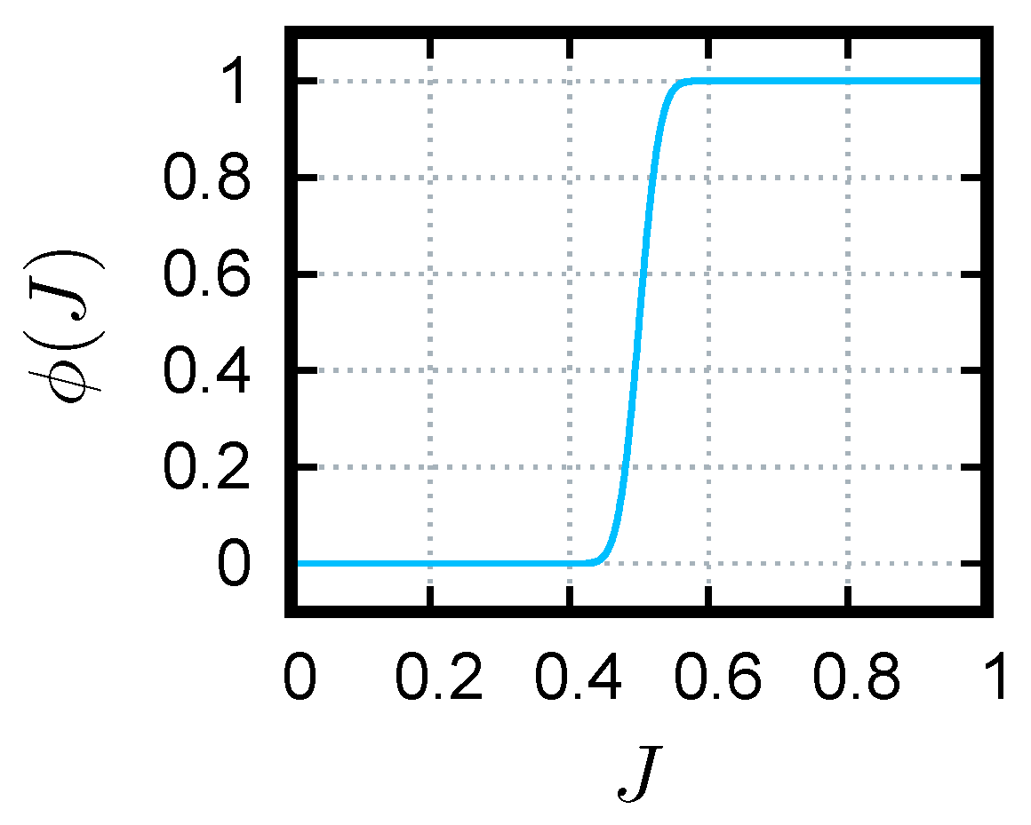
Therein, the almost smooth cutoff function is empirically defined by
which makes use of the well-known error function. The cutoff function is depicted in Figure 2. This reliability indicator could, in principle, be modified, e.g., the steepness, the smoothness, and its center could be adjusted. Thus, it should be regarded as an example only.
This weighted numerical quadrature rule is used henceforward for all numerical volume averaging operations. Its application will not be noted explicitly. However, the theoretical derivation of the RB method, as described in Section 2.1, is not affected by this, i.e., volume averaging operations remain exact as far as the theory is concerned. The two most important consequences of this numerical tweak are:
- The RB method is robust with respect to outlier values of the determinant. The modified quadrature rule extends the set of coefficient vectors for which effective quantities can be computed, albeit approximately, to the whole space .
- The significance of local fields varies with the value of the cutoff function. When attains values less than one, information is considered accordingly less reliable. In this sense, microscopic information is filtered based on a trust region for J defined by can be seen as a reliability indicator.
3. Sampling
3.1. General Considerations
The proposed sampling strategy builds on the previous work [12], in which the authors proposed an analogous sampling procedure for the small strain setting. However, substantial modifications are required in order to account for the finite rotational part, , of the macroscopic deformation gradient, , and the nonlinearity of the volumetric part of the deformation, J, with respect to the local displacements, u. For the setup of the Reduced Basis model as described in Section 2.2, the space of macroscopic deformation gradients,
needs to be sampled, i.e., the discrete sampling set is to be defined. Two contradictory requirements need to be satisfied when constructing :
- The samples should be densely and homogeneously distributed within the space of all admissible macroscopic kinematic configurations. This is owing to the desire that the POD may extract correlation information from a holistic and unbiased set. In other words, the samples should be as uniformly random as possible within the anticipated query domain of the surrogate.
- The sample number should not exceed a certain limit. Only with this property may the RB be identified within the bounds of available computational resources (e.g., memory and CPU time).
3.2. Large Strain Sampling Strategy
The set of admissible macroscopic deformation gradients is a subset of a nine-dimensional space () restricted by the inequality
Therefore, a regular grid in the components of might lead to a prohibitively large amount of samples, and even to a violation of (39). For instance, such a grid with a rather moderate resolution of just 10 samples of each component would require 1 billion solutions of the FOM. Also, the subsequent POD would involve a snapshot matrix and/or correlation matrix of accordingly huge dimensionality.
In order to decrease the dimension of the sampling space, recall the polar decomposition of the deformation gradient, , where is a rotation and is the symmetric positive definite (s.p.d.) stretch tensor. Material objectivity implies the energy function to be independent of the frame of reference,
and the transformation behavior
for the first Piola–Kirchhoff stress and
for the components of the corresponding stiffness tensor , see Appendix A. These known facts lead to
Note 2.
In order to collect representative samples of the hyperelastic response functions , , and , it suffices to evaluate them on samples of the stretch tensor instead of evaluating them on samples of the deformation gradient .
This effectively reduces the number of dimensions of from nine to six. The same dimensionality is attained when considering the response functions with respect to a symmetric measure of strain, e.g., as is done in [30] where the tangent stiffness is efficiently computed using a perturbation technique. However, such measures are unsuitable for reduction by means of the proposed RB method.
The remaining six-dimensional space of s.p.d. tensors is not linear but a convex cone (which does not include the zero element). Moreover, linearly combining elements within this space quickly leads to values of describing unphysically large changes in volume. For instance, equates to more than 100% volumetric extension, which is well beyond the regime of usual hyperelastic materials that are often nearly incompressible. On the other hand, 100% deviatoric strain is within the range of many standard materials, such as rubber. Hence, in order to describe the space of practically relevant stretch tensors, we propose to apply the DDMS to the macroscopic stretch tensor,
Let denote the manifold of unimodular macroscopic stretch tensors . The multiplicative split (43) is the basis for:
Proposition 1.
The set of practically relevant macroscopic stretch tensors can be sampled via sampling of both the macroscopic determinants,
and the macroscopic unimodular stretch tensors,
where and are the numbers of the samples. The sampling set is determined by the product set
The choice of the dilatational samples is relatively straightforward. For many common materials, the expected range of is rather narrow, so a few equisized or adaptive sub-intervals around deliver sufficient resolution.
For the space of unimodular s.p.d. matrices representing , basic results of Lie group theory can be exploited. We restrict to stating well-known facts that are necessary at this point. For more details, the interested reader is referred to standard text books, such as [31].
Corollary 1.
Let
be the tangent space and
be the manifold of unimodular s.p.d. matrices. The matrix exponential maps the tangent space bijectively onto the manifold,
The proof of this statement is standard, e.g., by means of the eigenvalue decomposition, and does not necessitate the reference to the abstract setting of Lie groups. In fact, all of the following arguments could be given without the notion of tangent spaces and manifolds. However, this notion is a fundamental concept in nonlinear mechanics. For a very descriptive and comprehensive work on this topic, the reader is referred to [32]. We choose to build upon this concept, as it comes along with vivid interpretations of the function spaces and .
The set is the set of matrix representations of the stretch tensors . The tangent space is the set of Hencky strains, which is linear. Hence, by virtue of the matrix exponential, the sampling of the nonlinear manifold can be reduced to the sampling of a linear space. Moreover, the restrictions of symmetry and zero trace render the tangent space five-dimensional. This property is, by definition, shared with the manifold .
The two-dimensional case is now addressed for the sake of visualization. In this setting, the nonlinearity of the manifold and the structure of the sampling set can be illustrated figuratively. With the subscript (2) denoting two-dimensional quantities, a basis of the tangent space is given by
The stretch tensors are obtained through
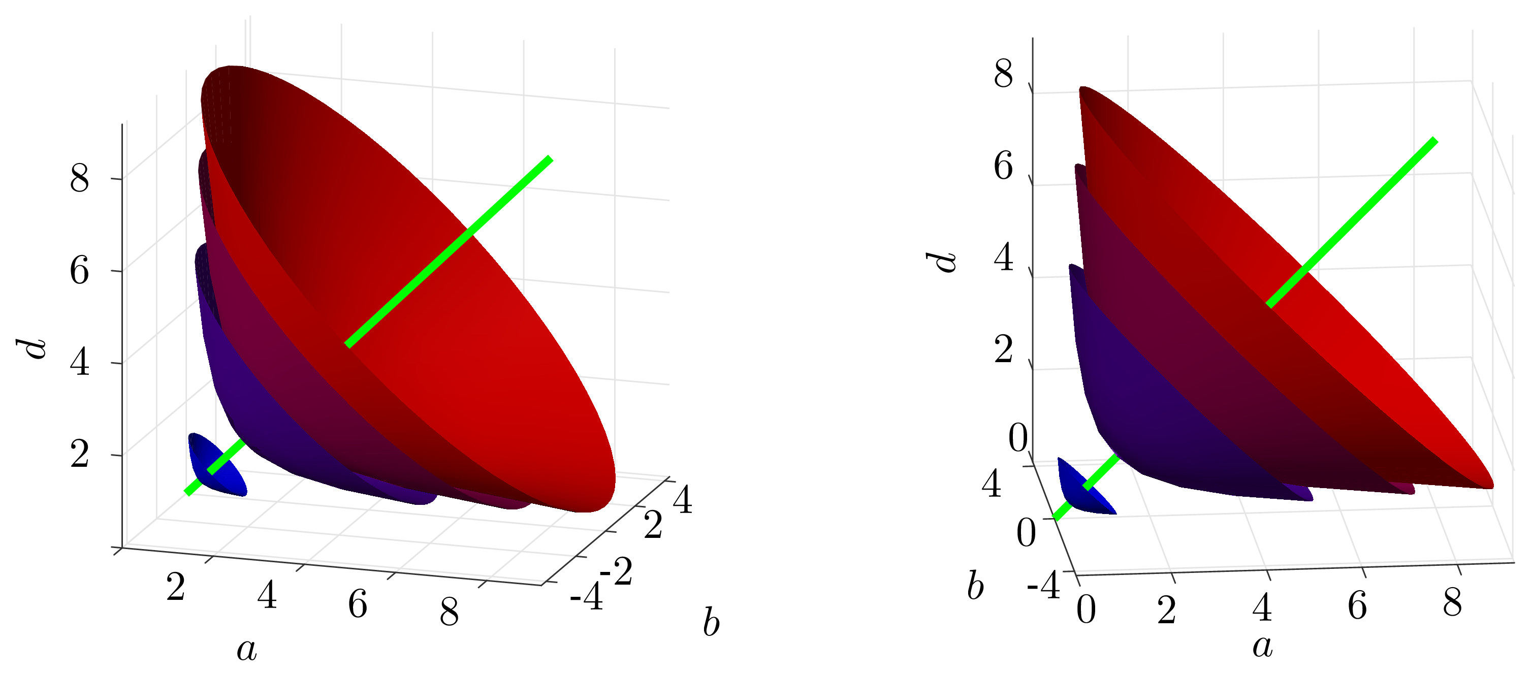
A visualization of such samples is depicted in Figure 3. There, for the sake of visual clarity, the determinant is sampled by four equidistant (and rather unrealistic) values between 0.1 and 4. The value is called deviatoric amplitude. A densely uniform sampling yields the coefficients and .
This emphasizes the important role of the DDMS in the context of sampling, as utilized in (44)—it allows for the identification of a physically meaningful sampling domain that is much smaller than the surrounding space of all admissible stretch tensors. On a side note, the isodet surfaces are perpendicular to the line representing the dilatational stretch tensors.
The proposed sampling procedure for in three dimensions is given in Algorithm 1. For this purpose, an orthonormal basis of the tangent space is fixed, cf. Appendix C. The numbers of different kind of samples , , and relate to the quantities and introduced in (44) by and .
| Algorithm 1: Sampling of the macroscopic stretch tensor. |
| Input : minimum and maximum determinant with maximum deviatoric amplitude number of macroscopic determinants number of deviatoric directions number of deviatoric amplitudes Output: samples of
|
The order of Steps 1 to 3 is interchangeable. Details on these parts are now presented:
- Step 1.
- Uniform seeding of the determinants is actually not required, but any pattern implying the sampling determinants to be dense in as works without loss of generality. In this way, the dilatational response may be resolved adaptively.
- Step 2.
- The generation of uniform point distributions on spheres is a research topic on its own, see [33] for an overview. The method described in [12] is based on energy minimization, which is also used in the present work. Some point sets of various sizes are included in the example program [18]. More detailed investigations on this topic and an open-source code of a point generation program are part of another work, [34]. Alternatively, Equal Area Points [35] may be used as a rough but quickly computable approximation of such point sets.
- Step 3.
- As in Step 1, the uniform placement of the deviatoric amplitudes, , may be substituted by adaptive alternatives. In [12], we have suggested to use an exponential distance function.
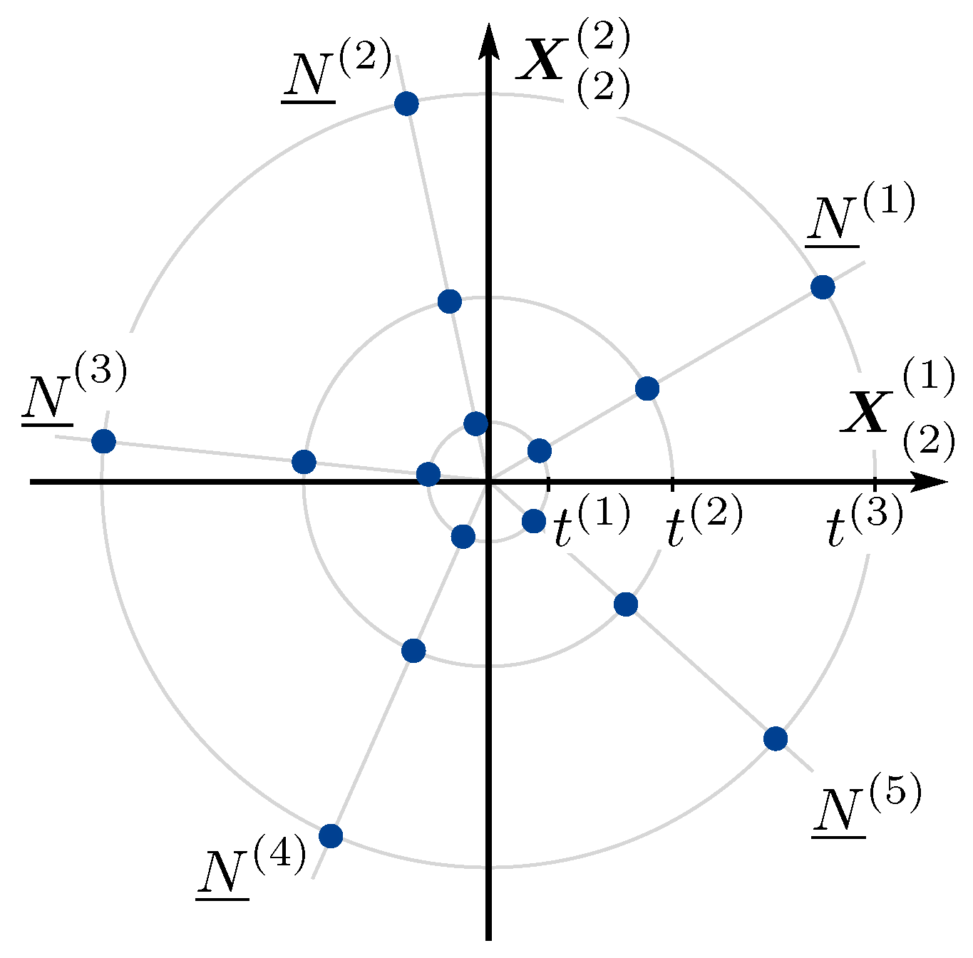
The result of Steps 2 and 3, i.e., the sampling of the tangent space, is exemplified in Figure 4 for the two-dimensional case () and for and . There, an adaptive spacing of the deviatoric amplitudes is applied. This might be beneficial for capturing strongly changing material behavior near the relaxed state.
In general, the vector , , corresponding to a macroscopic Hencky strain characterizes the direction of the applied stretch , which we also coin the load case.
3.3. Application of the Stretch Tensor Trained Reduced Basis Model
Since the RB model is trained on only the rotationally invariant part of but should be applied to general deformation gradients, the transformation rules (41) and (42) are incorporated during the evaluation of the surrogate model. Details on the procedure are given in Algorithm 2.
| Algorithm 2: Online phase of the stretch tensor trained Reduced Basis method |
| Input : macroscopic deformation gradient Output: , effective material response
|
4. Numerical Examples
4.1. Reduced Basis for a Fibrous Microstructure
The applicability of the proposed RB method in combination with the sampling scheme is now numerically studied for a fibrous microstructure roughly resembling polymers with woven reinforcements. The goal is to prove the efficiency of the F-RB scheme in principle and under “worst-case” conditions, the latter meaning that the phase contrast is chosen to be rather large. Yet, at this stage, it is explicitly not aspired to provide fully realistic examples. These would require investigations on the proper size of the microstructure and should employ dissipative material laws, both of which are not within the scope of this work.
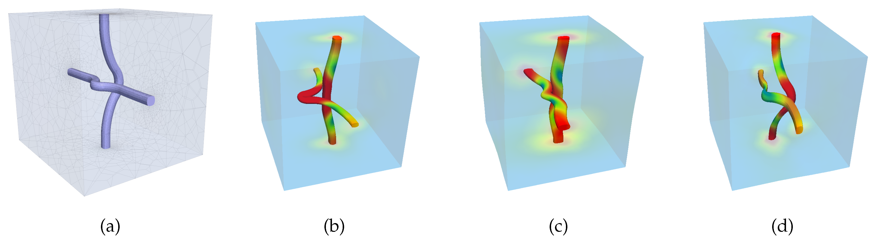
A cubical microstructure with two fibrous inclusions is considered, see Figure 5a and cf. [36] for a related example. The inclusions are periodic and occupy approximately 0.7% of the volume. The mesh contains 35,516 nodes in 25,633 quadratic tetrahedron elements (C3D10).
For the matrix, the material constants are chosen to be MPa and MPa, resembling rubber-like material properties. For the fibers, the values are MPa and MPa. The latter parameters approximate the behavior of stiffer polymers, such as polyethylene. The phase contrast is 600 with respect to the shear moduli, and the Poisson ratios are and .
The training boundary conditions are defined with deviatoric directions, , and deviatoric amplitudes, , which are regularly distributed in the interval . In order to also consider response to volumetric extension in the training data, an additional set of = 10 boundary conditions of the form is included in the training set, with the determinant being linearly increased from 1 to 1.02.
The validation load cases are 640 mixed dilatational-deviatoric boundary conditions. Along new deviatoric directions, both the deviatoric amplitudes () and the dilatational amplitudes () are applied in 10 equidistant increments.
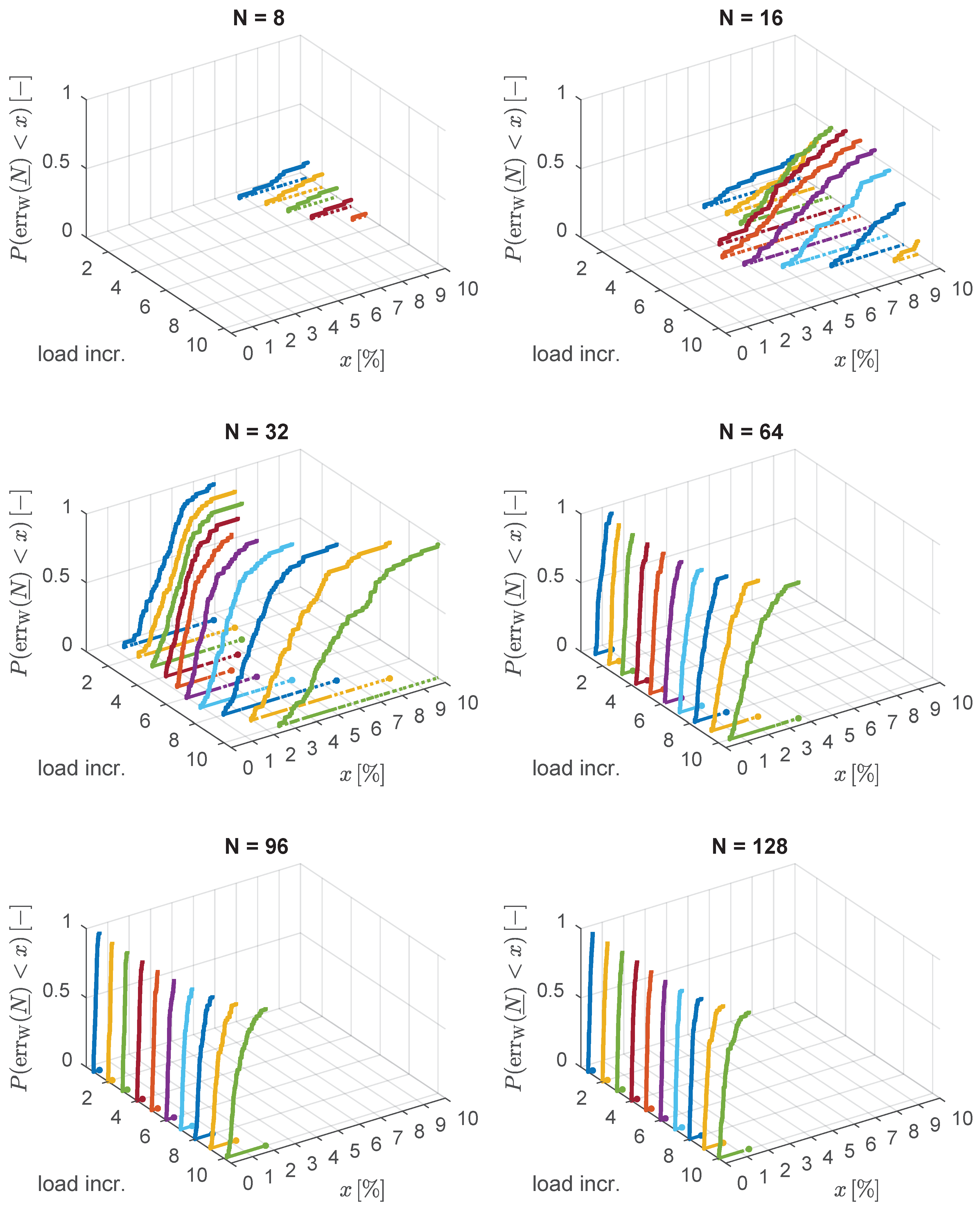
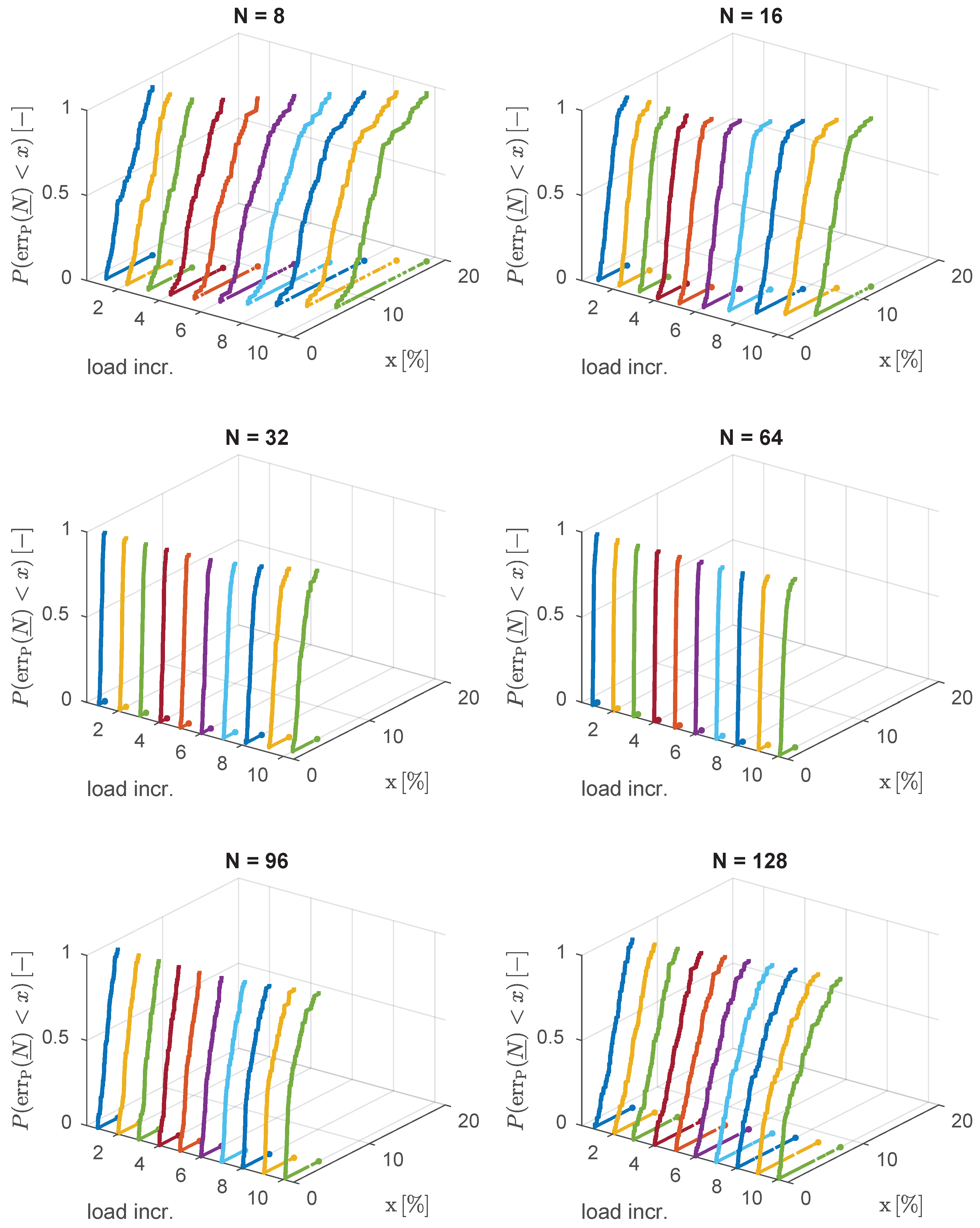
The results for various values N of the RB-size are compared with the results of FE simulations with the same boundary conditions. To this end, the error measures
are employed. Figure 6 and Figure 7 visualize the results.
The distribution of the energy error, , improves monotonically as the RB is enriched from to elements. This enrichment corresponds to the inclusion of additional subtrahends in the computation of , improving the spectral over-estimation by the volume average of the stiffness, cf. (17). It is also noteworthy that the error tends to be higher for larger magnitudes of the applied kinematic boundary condition, although that is not always the case.
In contrast to this, the stress error distribution monotonically improves only up to a certain threshold value of the number of basis elements, which is in this example. For the greater bases with and , the quality of the results deteriorates as far as the stress error is concerned. This is most likely due to an excessively oscillatory nature of the higher order modes—at some critical level , the POD constructs eigenvectors with the -norm . Therefore, the POD would construct basis vectors out of numerical fluctuations, which would be unphysical. While the enrichment of the optimization space with unphysical information cannot increase the minimum energy error , it might lead to fluctuations in the displacement field that have significant impact on the overall stress response. This is especially the case for numerical fluctuations within the stiff inclusion phase where low overall displacement errors still could lead to notable impact on the effective stress.
Nonetheless, all observed errors are less than 20% and stay below 3% for the optimal sampled size . For half the basis size, , the errors max at approximately 5%, which is still acceptable considering the uncertainties involved in realistic two-scale simulations. Note that the maximum errors strongly depend on the maximum load amplitude, which is chosen to be very large in this example (50% deviatoric strain and 0.5% compression).
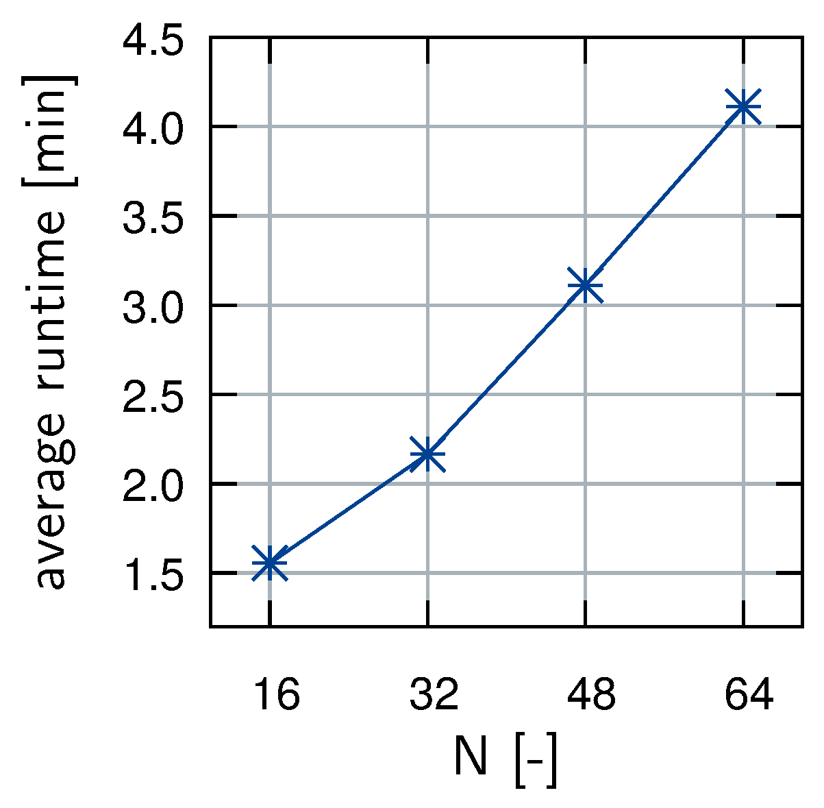
The runtimes of the RB model for different sizes N are depicted in Figure 8. A nearly linear growth of the runtime with respect to the basis size can be asserted. It is noteworthy that the online time of the RB method is strongly dominated by the assembly of the Jacobian . Therefore, a Quasi-Newton implementation was chosen, resulting in only two assemblies per load increment.
Speed-ups become impressive when very large load increments are considered. In all examples observed thus far, the RB converges to the final load amplitude in a single increment, requiring 7–13 Quasi–Newton iterations, with only 2–4 assemblies of the Jacobi matrix and a runtime of 10–50 seconds. This is in strong contrast to the FEM which is very sensitive to large load increments as they come along with a high probability of a violation of the condition . By means of standard implementation, such occurrences are usually treated with cutbacks of the load increment, which is detrimental to the runtime of the FEM.
No rigorous speed-up analysis is intended at this point. Both the codes of the FEM and of the RB method are fairly efficient in-house C/C++ developments and perform exact line searches. While the FEM has not yet been equipped with a Quasi–Newton procedure, the linear solver makes use of parallelization. This is in contrary to the current implementation of the RB method. Depending on the microstructure (especially the geometry, material nonlinearities, and phase contrast), the loading conditions, and the size N of the RB, speed-up factors are in the order of 5–100.
4.2. Reduced Basis for a Stiffening Microstructure
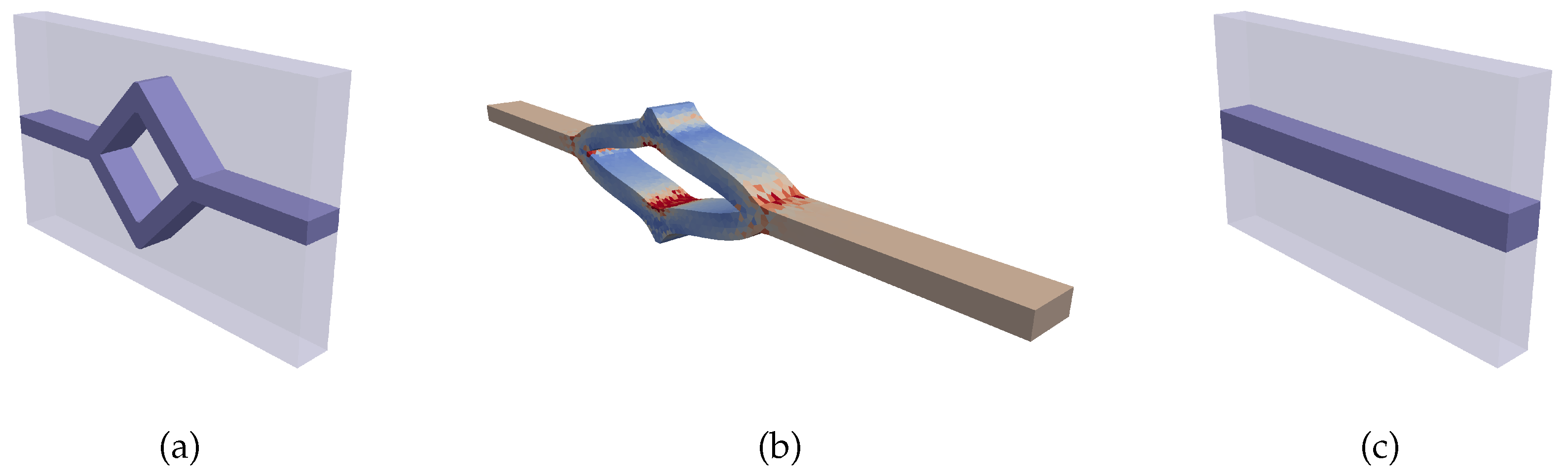
The second example takes the “worst-case” approach further by considering a noncubical microstructure with even higher phase contrast and significant topological nonlinearity. To this end, a cuboid microstructure occupying the domain and containing a hash-like inclusion is investigated, see Figure 9a. The mesh is periodic and contains 33,923 nodes in 21,726 quadratic tetrahedron elements (C3D10). The reinforcement makes up approximately 13.3% of the volume. Due to this large volume fraction, a pronounced geometry-induced nonlinearity of the effective response is expected under uniaxial loading conditions along the x-axis. As it is elongated, the hashlike part is straightened and thus increasingly aligned with the external loading, see Figure 9b. Such effects might be desirable when designing microstructures for functional materials.
The material parameters are MPa, MPa, MPa, and MPa, implying a Poisson ratio of in both materials and a phase contrast of 1000.
The training boundary conditions are the deviatoric ones of the set considered in Section 4.1, i.e., deviatoric directions and regularly spaced deviatoric amplitudes from the interval . No dilatational training cases are considered, i.e., only points from a five-dimensional submanifold of the space are sampled.
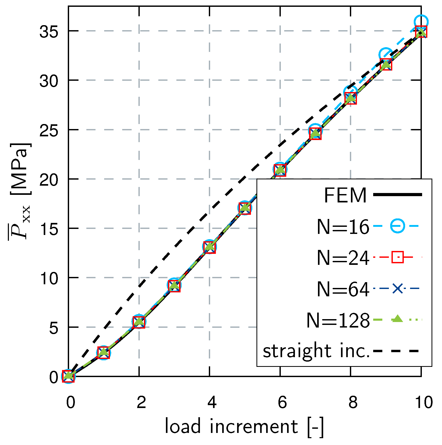
Uniaxial tension boundary conditions are applied for the validation. More precisely, the stretch component is increased from to in 10 increments of equal size. The other components are chosen such that all but the -component of the effective stress vanish.
Figure 10 depicts the results for different sizes N of the RB. The influence of the stiffening effect on the stress curve is emphasized by the black dashed line corresponding to a similar microstructure with a straight, cuboid inclusion that leads to the same final stress value under these boundary conditions, see Figure 9c.
In this example, the geometric stiffening effect is captured by the RB with high accuracy, with as few as basis elements. For moderate stretches, even an RB size of suffices. These results are somewhat more impressive when noticing that the applied boundary condition contains more than 1.2% volumetric compression, i.e. the validation loading actually lies outside the submanifold covered during training.
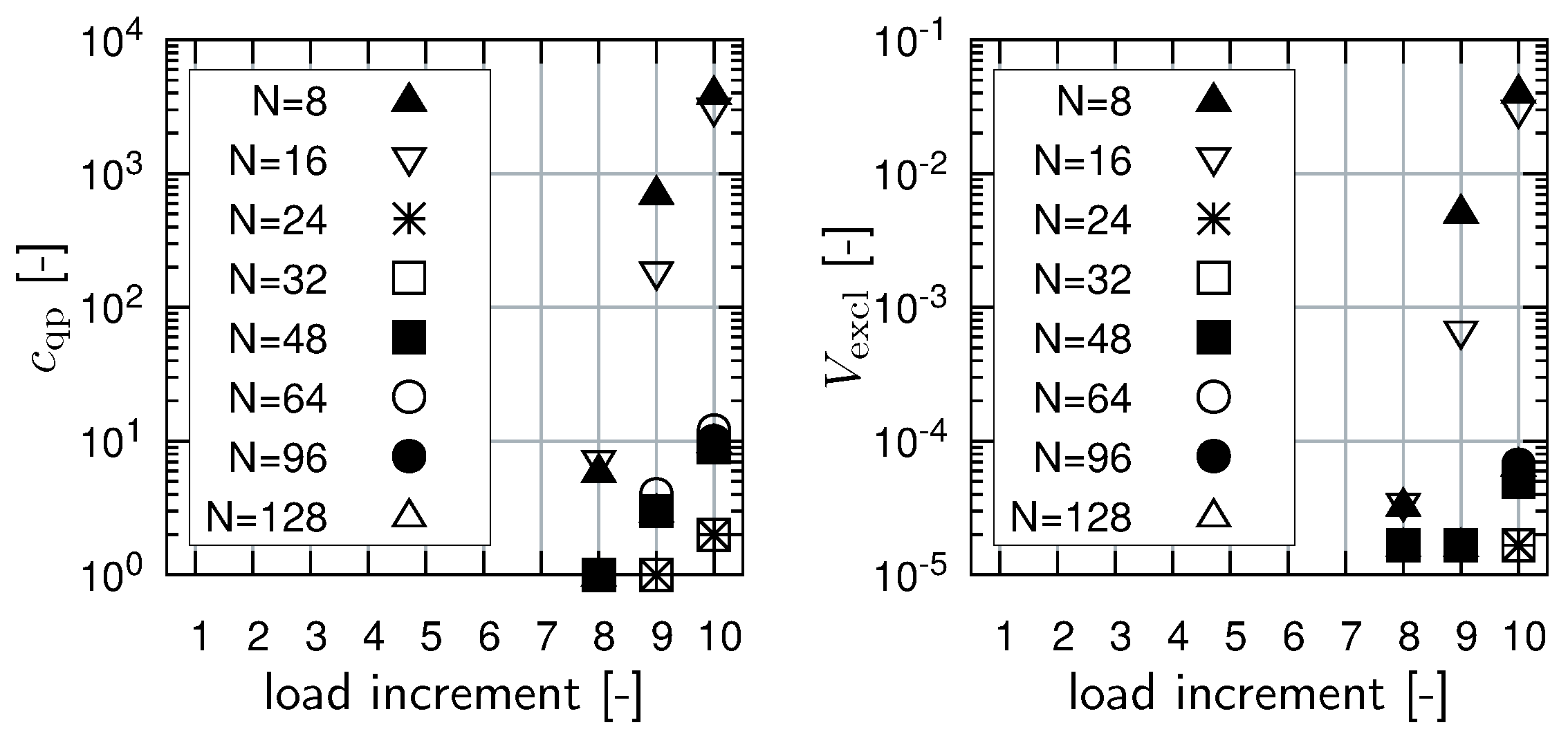
In order to examine the action of the cutoff function ϕ, the following two indicators are introduced:
The first quantity, , counts the number of quadrature points at which the cutoff function has an influence. The second one, , measures the relative excluded volume, interpreting the value of ϕ as a scaling of the corresponding quadrature weight. The values of these indicators are depicted in Figure 11.
Most notably, the cutoff function does not have any effect before the eighth load increment in this example. Only for large load amplitudes does this numerical stability tweak become necessary. Even then, the number of points at which it has an influence is small, considering the total number of quadrature points, . This example is representative for all conducted numerical experiments.
5. Discussion
5.1. Discussion of the Reduced Basis Method
5.1.1. Relation of the RB Homogenization to Analytical Estimates
Zero coefficients, , correspond to the Taylor homogenization, i.e., to the nonlinear counterpart of the Voigt estimate [37], which provides an upper bound for the material response, cf. (17). Starting with the initial guess , the evolution of the coefficients corresponds to a (possibly not monotonous) relaxation of this overly stiff response into a more natural state. In view of improved computational efficiency, a nonzero initial guess combined with an exact line search has proven reasonable and easy to realize. For instance, such a guess might stem from previous load steps or an interpolation/extrapolation of available coefficient data.
5.1.2. Reconstruction of Displacement Fields
Given an RB approximation of the deformation gradient, , one can reconstruct the corresponding displacement field uniquely up to rigid body motion. This is possible due to the linear dependence of the deformation gradient fluctuations on the displacement fluctuations. Recall the definition of the RB in (32),
The corresponding displacement fluctuations are
The displacement fluctuation fields are defined by , where the displacement fields are the solutions computed during training, and . Thus, a displacement field compatible to the RB result is given by
The missing term , cf. (10), cannot be reconstructed.
5.1.3. Relation to Classical Displacement-Based POD Methods
In a certain sense, the entries of the correlation matrix used in the offline phase, cf. Section 2.2, are “weighted” scalar products of the displacement fluctuation fields within the Sobolev space . “Weighted” is to be understood in that the zeroth order derivative is multiplied by zero. Classical displacement-based POD methods compute correlations of the fluctuations within the Lebesgue space . The change to -like scalar products is physically motivated by the fact that the local energy explicitly depends on the gradient of the displacement, , but not on the displacement, u.
5.1.4. Advantages Compared to General Displacement-Based Schemes
The proposed method is advantageous compared to both displacement-based POD methods and the classical FEM for the following reasons:
- No gradients need to be computed from displacement fields, which displacement-based schemes always require prior to the evaluation of the material law.
- The residual and the Jacobian are algorithmically sleek and trivial to implement.
- The absence of element formulations in the assembly of the reduced residual and of the Jacobi matrix contributes to both the simplicity and the efficiency of the method—no incidence matrices occur, allowing for linear memory access. Moreover, the algebraic operations associated with reference element formulations are bypassed. This is also in favor of parallel computations. Such an implementation is still outstanding for the problem at hand, but has been conducted for related problems in the small strain setting in [38].
Although the storage of the basis requires double precision values, the basis is compact enough to be completely loaded into random access memory of standard computers. For instance, the bases considered in Section 4 occupy only ~200 Mb of memory for .
We now briefly address the algorithmic complexity associated with the proposed F-RB method and with the u-RB method that was employed in previous works, such as [9] and [8]. To this end, the fully discretized versions of the residual and of the Jacobian as well as discrete quantities associated with the u-RB method are introduced in the following listing.
- : Nine values of the stress at the quadrature point
- : Symmetric stiffness tensor
- : F-RB matrix containing the nine values of each basis elements as columns
- : The quadrature weight at
- : Three times the number of nodes,
- : Global FE residual vector
- : u-RB matrix of which the columns contain the nodal displacement values
- : Global FE stiffness matrix
Table 1 compares the algorithmic complexity of the presented F-RB method with that of standard u-RB schemes. First of all, both methods share a quadratic dependence of their Jacobi matrices on the number of modes, N. Therefore, the assembly of the Jacobian is usually the most costly operation. Secondly, both approaches’ complexities suffer a linear dependency on the number of quadrature points, . In the displacement-based approach, this is included in the assembly of the residual and of the stiffness, which relate to the factor 9 and 92, respectively. Thirdly, the novel F-RB scheme spares the computational overhead associated with FE formulations and . More details on this matter are currently being investigated.
5.1.5. Outlook
Future research should aim at an application of the introduced Reduced Basis method within realistic two-scale simulations, in analog to [12,38,39,40]. Hyperreduction methods, cf. [41], might give rise to additional speed-ups in the online phase. Further, modifications of the cutoff function, ϕ, should be investigated—a function with compact support might be more appropriate. The construction of the RB from large sets of snapshots is computationally intense, as much data needs to be processed. In the above examples, the POD consumed multiple hours of time. Hierarchical approximations, such as [42], might mitigate the effects by enabling parallel computations. Overall, the long-term perspective is to extend this RB framework efficiently to the context of dissipative materials.
5.2. Discussion of the Sampling Strategy
The proposed sampling strategy is meant to serve as a template. As exemplified in Section 4.1, the samplings can be modified and still lead to a coverage of the set of macroscopic boundary conditions that is sufficient for the problem at hand. The example of Section 4.2 took this idea further and showed that it might not even be necessary to sample the macroscopic determinant. Hence, the sampling can sometimes be reduced to the five-dimensional subspace of isochoric macroscopic stretch tensors.
In any case, the exact choice of both the inputs to Algorithm 1 and the distributions of the deviatoric amplitudes and the macroscopic determinants remains to be based on knowledge and sophisticated guesses, at least at the current state of the art. Further research on this matter might lead to a refined alternative to Algorithm 1, possibly involving the evaluation of error estimators.
Author Contributions
Conceptualization, O.K. and F.F.; Funding acquisition, F.F.; Methodology, O.K. and F.F.; Project administration, F.F.; Software, O.K.; Supervision, F.F.; Writing—original draft, O.K. and F.F.
Funding
This research was funded by Deutsche Forschungsgemeinschaft (DFG) within the Emmy–Noether programm under grant DFG-FR2702/6.
Conflicts of Interest
The authors declare no conflict of interest.
Abbreviations
The following abbreviations are used in this manuscript:
| RB | Reduced Basis |
| FE(M) | Finite Element (Method) |
| POD | Proper Orthogonal Decomposition |
| DOF | degree(s) of freedom |
| FOM | full-order model |
| s.p.d. | symmetric positive definite |
| DDMS | Dilatational-Deviatoric Multiplicative Split |
Appendix A. Material Objectivity
The transformation behavior of the components of the stiffness tensor is now deduced. To this end, Green’s strain tensor , the corresponding stored energy density function , the second Piola–Kirchhoff stress , and the corresponding stiffness tensor are introduced. Starting from the well-known relationship between and the first Piola–Kirchhoff stress (see for instance [43]), we express the components of in terms of those of and of :
Here, is the Kronecker symbol. In the last step, the minor symmetry has been exploited, and above and throughout. From this, the inverse relation
can be derived. The fact that Green’s strain tensor is frame invariant, i.e., , implies that both the left hand side and the second Piola–Kirchhoff stress are independent of . This is in contrast to from which follows that
By contraction of the indices i and k with the second index of and the first index of , respectively, Equation (42) follows.
Appendix B. Effective Material Responses of the RB
Let denote the fourth order identity tensor and let the arguments of the F-RB approximation (23) be omitted, i.e., here . Its derivative with respect to the boundary condition is
Appendix B.1. Effective Stress
Appendix B.2. Effective Stiffness
For , we demand that the residual from (28) is stable with respect to the boundary condition when converged to ,
It follows that
Appendix C. Basis for Symmetric Traceless Second Order Tensors
References
- Rendek, M.; Lion, A. Amplitude dependence of filler-reinforced rubber: Experiments, constitutive modelling and FEM—Implementation. Int. J. Solids Struct. 2010, 47, 2918–2936. [Google Scholar] [CrossRef]
- Nguyen, V.D.; Lani, F.; Pardoen, T.; Morelle, X.; Noels, L. A large strain hyperelastic viscoelastic-viscoplastic-damage constitutive model based on a multi-mechanism non-local damage continuum for amorphous glassy polymers. Int. J. Solids Struct. 2016, 96, 192–216. [Google Scholar] [CrossRef] [Green Version]
- Barrault, M.; Maday, Y.; Nguyen, N.C.; Patera, A.T. An ‘empirical interpolation’ method: Application to efficient reduced-basis discretization of partial differential equations. C. R. Math. 2004, 339, 667–672. [Google Scholar] [CrossRef]
- Geers, M.; Yvonnet, J. Multiscale modeling of microstructure-property relations. MRS Bull. 2016, 41, 610–616. [Google Scholar] [CrossRef]
- Saeb, S.; Steinmann, P.; Javili, A. Aspects of Computational Homogenization at Finite Deformations: A Unifying Review From Reuss’ to Voigt’s Bound. Appl. Mech. Rev. 2016, 68, 050801. [Google Scholar] [CrossRef]
- Feyel, F. Multiscale FE2 elastoviscoplastic analysis of composite structures. Comput. Mater. Sci. 1999, 16, 344–354. [Google Scholar] [CrossRef]
- Sirovich, L. Turbulence and the Dynamics of Coherent Structures. Part 1: Coherent Structures. Q. Appl. Math. 1987, 45, 561–571. [Google Scholar] [CrossRef]
- Yvonnet, J.; He, Q.C. The reduced model multiscale method (R3M) for the non-linear homogenization of hyperelastic media at finite strains. J. Comput. Phys. 2007, 223, 341–368. [Google Scholar] [CrossRef] [Green Version]
- Radermacher, A.; Reese, S. POD-based model reduction with empirical interpolation applied to nonlinear elasticity. Int. J. Numer. Methods Eng. 2016, 107, 477–495. [Google Scholar] [CrossRef]
- Radermacher, A.; Reese, S. Proper orthogonal decomposition-based model reduction for non-linear biomechanical analysis. Int. J. Mater. Eng. Innov. 2013, 4, 149–165. [Google Scholar] [CrossRef]
- Soldner, D.; Brands, B.; Zabihyan, R.; Steinmann, P.; Mergheim, J. A numerical study of different projection-based model reduction techniques applied to computational homogenisation. Comput. Mech. 2017, 60, 613–625. [Google Scholar] [CrossRef] [Green Version]
- Fritzen, F.; Kunc, O. Two-stage data-driven homogenization for nonlinear solids using a reduced order model. Eur. J. Mech. A Solids 2018, 69, 201–220. [Google Scholar] [CrossRef]
- Akkari, N.; Casenave, F.; Moureau, V. Time Stable Reduced Order Modeling by an Enhanced Reduced Order Basis of the Turbulent and Incompressible 3D Navier–Stokes Equations. Math. Comput. Appl. 2019, 24, 45. [Google Scholar] [CrossRef]
- An, S.; Kim, T.; James, D.L. Optimizing cubature for efficient integration of subspace deformations. ACM Trans. Graph. 2009, 27, 165:1–165:10. [Google Scholar] [CrossRef]
- Hernández, J.; Caicedo, M.; Ferrer, A. Dimensional hyper-reduction of nonlinear finite element models via empirical cubature. Comput. Methods Appl. Mech. Eng. 2017, 313, 687–722. [Google Scholar] [CrossRef] [Green Version]
- Temizer, I.; Zohdi, T. A numerical method for homogenization in non-linear elasticity. Comput. Mech. 2007, 40, 281–298. [Google Scholar] [CrossRef]
- Yvonnet, J.; Monteiro, E.; He, Q.C. Computational homogenization method and reduced database model for hyperelastic heterogeneous structures. J. Multiscale Comput. Eng. 2013, 11, 201–225. [Google Scholar] [CrossRef]
- Kunc, O. GitHub repository ReducedBasisDemonstrator. Available online: https://github.com/EMMA-Group/ReducedBasisDemonstrator (accessed on 27 May 2019).
- Flory, P. Thermodynamic relations for high elastic materials. Trans. Faraday Soc. 1961, 57, 829–838. [Google Scholar] [CrossRef]
- Bilger, N.; Auslender, F.; Bornert, M.; Michel, J.C.; Moulinec, H.; Suquet, P.; Zaoui, A. Effect of a nonuniform distribution of voids on the plastic response of voided materials: a computational and statistical analysis. Int. J. Solids Struct. 2005, 42, 517–538. [Google Scholar] [CrossRef] [Green Version]
- Doll, S.; Schweizerhof, K. On the Development of Volumetric Strain Energy Functions. J. Appl. Mech. 1999, 67, 17–21. [Google Scholar] [CrossRef] [Green Version]
- Simo, J. A framework for finite strain elastoplasticity based on maximum plastic dissipation and the multiplicative decomposition: Part I. Continuum formulation. Comput. Methods Appl. Mech. Eng. 1988, 66, 199–219. [Google Scholar] [CrossRef]
- Pruchnicki, E. Hyperelastic homogenized law for reinforced elastomer at finite strain with edge effects. Acta Mech. 1998, 129, 139–162. [Google Scholar] [CrossRef]
- Miehe, C. Computational micro-to-macro transitions for discretized micro-structures of heterogeneous materials at finite strains based on the minimization of averaged incremental energy. Comput. Methods Appl. Mech. Eng. 2003, 192, 559–591. [Google Scholar] [CrossRef]
- Castañeda, P.P.; Suquet, P. Nonlinear Composites. Adv. Appl. Mech. 1998, 34, 172–302. [Google Scholar] [CrossRef]
- Kabel, M.; Böhlke, T.; Schneider, M. Efficient fixed point and Newton–Krylov solvers for FFT-based homogenization of elasticity at large deformations. Comput. Mech. 2014, 54, 1497–1514. [Google Scholar] [CrossRef]
- Quarteroni, A.; Manzoni, A.; Negri, F. Reduced Basis Methods for Partial Differential Equations: An Introduction; Springer: Cham, Switzerland, 2016. [Google Scholar]
- Ball, J.M. Convexity conditions and existence theorems in nonlinear elasticity. Arch. Ration. Mech. Anal. 1976, 63, 337–403. [Google Scholar] [CrossRef]
- Schneider, M. Beyond polyconvexity: An existence result for a class of quasiconvex hyperelastic materials. Math. Methods Appl. Sci. 2017, 40, 2084–2089. [Google Scholar] [CrossRef]
- Miehe, C. Numerical computation of algorithmic (consistent) tangent moduli in large-strain computational inelasticity. Comput. Methods Appl. Mech. Eng. 1996, 134, 223–240. [Google Scholar] [CrossRef]
- Faraut, J. Analysis on Lie Groups: An Introduction; Cambridge University Press: Cambridge, UK, 2008. [Google Scholar]
- Neff, P.; Eidel, B.; Martin, R.J. Geometry of Logarithmic Strain Measures in Solid Mechanics. Arch. Ration. Mech. Anal. 2016, 222, 507–572. [Google Scholar] [CrossRef] [Green Version]
- Brauchart, J.S.; Grabner, P.J. Distributing many points on spheres: Minimal energy and designs. J. Complex. 2015, 31, 293–326. [Google Scholar] [CrossRef] [Green Version]
- Kunc, O.; Fritzen, F. Generation of energy-minimizing point sets on spheres and their application in mesh-free interpolation and differentiation. Adv. Comput. Math. 2018. Under review. [Google Scholar]
- Leopardi, P. A partition of the unit sphere into regions of equal area and small diameter. Electron. Trans. Numer. Anal. 2006, 25, 309–327. [Google Scholar]
- Kim, H.J.; Swan, C.C. Algorithms for automated meshing and unit cell analysis of periodic composites with hierarchical tri-quadratic tetrahedral elements. Int. J. Numer. Methods Eng. 2003, 58, 1683–1711. [Google Scholar] [CrossRef]
- Voigt, W. Lehrbuch der Kristallphysik; Vieweg+Teubner Verlag: Wiesbaden, Germany, 1966. [Google Scholar]
- Fritzen, F.; Hodapp, M. The finite element square reduced (FE2R) method with GPU acceleration: Towards three-dimensional two-scale simulations. Int. J. Numer. Methods Eng. 2016, 107, 853–881. [Google Scholar] [CrossRef]
- Rambausek, M.; Göküzüm, F.S.; Nguyen, L.T.K.; Keip, M.A. A two-scale FE-FFT approach to nonlinear magneto-elasticity. Int. J. Numer. Methods Eng. 2019, 117, 1117–1142. [Google Scholar] [CrossRef]
- Kochmann, J.; Wulfinghoff, S.; Ehle, L.; Mayer, J.; Svendsen, B.; Reese, S. Efficient and accurate two-scale FE-FFT-based prediction of the effective material behavior of elasto-viscoplastic polycrystals. Comput. Mech. 2017. [Google Scholar] [CrossRef]
- Ryckelynck, D. A priori hyperreduction method: an adaptive approach. J. Comput. Phys. 2005, 202, 346–366. [Google Scholar] [CrossRef] [Green Version]
- Himpe, C.; Leibner, T.; Rave, S. Hierarchical Approximate Proper Orthogonal Decomposition. SIAM J. Sci. Comput. 2018, 40, A3267–A3292. [Google Scholar] [CrossRef] [Green Version]
- Bertram, A. Elasticity and Plasticity of Large Deformations; Springer: Berlin/Heidelberg, Germany, 2008. [Google Scholar] [CrossRef]
Figure 1.
Initial () and current () configuration, with elementary kinematic quantities.

Figure 2.
Cutoff function . Its value is used as a reliability factor in the numerical quadrature.

Figure 3.
Visualizations of the family of -manifolds with constant determinant for the two-dimensional case from two different perspectives. The green line represents the set .
Figure 3.
Visualizations of the family of -manifolds with constant determinant for the two-dimensional case from two different perspectives. The green line represents the set .

Figure 4.
Example of a discretization of the two-dimensional tangent space. The samples are placed along the equidistant (in higher dimensions—uniformly distributed) directions with nonuniformly increasing amplitude.
Figure 4.
Example of a discretization of the two-dimensional tangent space. The samples are placed along the equidistant (in higher dimensions—uniformly distributed) directions with nonuniformly increasing amplitude.

Figure 5.
(a) fibrous microstructure. (b–d) random F-reduced basis (RB) elements.

Figure 6.
Cumulative energy error distribution per direction for the RB of the fibrous microstructure under validation boundary conditions.
Figure 6.
Cumulative energy error distribution per direction for the RB of the fibrous microstructure under validation boundary conditions.

Figure 7.
Cumulative stress error distribution per direction for the RB of the fibrous microstructure under validation boundary conditions.
Figure 7.
Cumulative stress error distribution per direction for the RB of the fibrous microstructure under validation boundary conditions.

Figure 8.
Laptop computer runtimes of the RB model for the fibrous microstructure for various sizes N of the basis. Each data point represents the time needed for all 10 load increments. The spread of the individual times of the 64 validation cases around these average values is negligible.
Figure 8.
Laptop computer runtimes of the RB model for the fibrous microstructure for various sizes N of the basis. Each data point represents the time needed for all 10 load increments. The spread of the individual times of the 64 validation cases around these average values is negligible.

Figure 9.
(a) Cuboidal microstructure with hashlike inclusion phase. (b) Deformed state under uniaxial tension loading. Only inclusion is shown, coloring indicates . (c) Straight inclusion substitute microstructure, leading to a comparable effective stress.
Figure 9.
(a) Cuboidal microstructure with hashlike inclusion phase. (b) Deformed state under uniaxial tension loading. Only inclusion is shown, coloring indicates . (c) Straight inclusion substitute microstructure, leading to a comparable effective stress.

Figure 10.
Stress curves for a microstructure with geometric stiffening (cf. Figure 9a), comparing the FEM result to the RB for various number of basis elements N. A similar microstructure without geometric stiffening but with the same final stress value (cf. Figure 9c) leads to the black dashed curve.

Figure 11.
(Left) Number of quadrature points at which the cutoff function ϕ attains a value less than one. (Right) Relative excluded volume.
Figure 11.
(Left) Number of quadrature points at which the cutoff function ϕ attains a value less than one. (Right) Relative excluded volume.


Table 1.
Algorithmic complexities of the well-established u-based RB method and the novel F-based RB method. The assembly of the FE residual and of the FE stiffness depend on .
Table 1.
Algorithmic complexities of the well-established u-based RB method and the novel F-based RB method. The assembly of the FE residual and of the FE stiffness depend on .
| RB Method | Quantity | Complexity |
|---|---|---|
| F-based | ||
| u-based | + assembly of | |
| + assembly of |
© 2019 by the authors. Licensee MDPI, Basel, Switzerland. This article is an open access article distributed under the terms and conditions of the Creative Commons Attribution (CC BY) license (http://creativecommons.org/licenses/by/4.0/).
Share and Cite
MDPI and ACS Style
Kunc, O.; Fritzen, F. Finite Strain Homogenization Using a Reduced Basis and Efficient Sampling. Math. Comput. Appl. 2019, 24, 56. https://doi.org/10.3390/mca24020056
AMA Style
Kunc O, Fritzen F. Finite Strain Homogenization Using a Reduced Basis and Efficient Sampling. Mathematical and Computational Applications. 2019; 24(2):56. https://doi.org/10.3390/mca24020056
Chicago/Turabian StyleKunc, Oliver, and Felix Fritzen. 2019. "Finite Strain Homogenization Using a Reduced Basis and Efficient Sampling" Mathematical and Computational Applications 24, no. 2: 56. https://doi.org/10.3390/mca24020056