k-Nearest Neighbor Learning with Graph Neural Networks

Abstract

k-nearest neighbor (kNN) is a widely used learning algorithm for supervised learning tasks. In practice, the main challenge when using kNN is its high sensitivity to its hyperparameter setting, including the number of nearest neighbors k, the distance function, and the weighting function. To improve the robustness to hyperparameters, this study presents a novel kNN learning method based on a graph neural network, named kNNGNN. Given training data, the method learns a task-specific kNN rule in an end-to-end fashion by means of a graph neural network that takes the kNN graph of an instance to predict the label of the instance. The distance and weighting functions are implicitly embedded within the graph neural network. For a query instance, the prediction is obtained by performing a kNN search from the training data to create a kNN graph and passing it through the graph neural network. The effectiveness of the proposed method is demonstrated using various benchmark datasets for classification and regression tasks.

1. Introduction

The k-nearest neighbor (kNN) algorithm is one of the most widely used learning algorithms in machine learning research [1,2]. The main concept of kNN is to predict the label of a query instance based on the labels of k closest instances in the stored data, assuming that the label of an instance is similar to that of its kNN instances. kNN is simple and easy to implement, but is very effective in terms of prediction performance. kNN makes no specific assumptions about the distribution of the data. Because it is an instance-based learning algorithm that requires no training before making predictions, incremental learning can be easily adopted. For these reasons, kNN has been actively applied to a variety of supervised learning tasks including both classification and regression tasks.

The procedure for kNN learning is as follows. Suppose a training dataset $\mathcal{D}={\left\{({\mathbf{x}}_t,{\mathbf{y}}_t)\right\}}_{t=1}^N$ is given for a supervised learning task, where ${\mathbf{x}}_t$ and ${\mathbf{y}}_t$ are the input vector and the corresponding label vector of the t-th instance. ${\mathbf{y}}_t$ is assumed to be a one-hot vector in the case of a classification task and a scalar value in the case of a regression task. In the training phase, the dataset $\mathcal{D}$ is just stored without any explicit learning from the dataset. In the inference phase, for each query instance $\mathbf{x}$, kNN search is performed to retrieve kNN instances $\mathcal{N}\left({\mathbf{x}}_t\right)={\left\{({\mathbf{x}}_t^{\left(i\right)},{\mathbf{y}}_t^{\left(i\right)})\right\}}_{i=1}^k$ that are closest to $\mathbf{x}$ based on a distance function d. Then, the predicted label $\widehat{\mathbf{y}}$ is obtained as a weighted combination of the labels ${\mathbf{y}}^{\left(1\right)},\dots ,{\mathbf{y}}^{\left(k\right)}$ based on a weighting function w along with the distance function d as follows:

$$\begin{array}{c}\hfill \widehat{\mathbf{y}}=f(\mathbf{x};\mathcal{D})=\frac{{\sum }_{i=1}^{k}w\left(d(\mathbf{x},{\mathbf{x}}^{\left(i\right)})\right)·{\mathbf{y}}^{\left(i\right)}}{{\sum }_{i=1}^{k}w\left(d(\mathbf{x},{\mathbf{x}}^{\left(i\right)})\right)}\end{array}$$

(1)

The difficulty in using kNN is determining the hyperparameters. The three main hyperparameters are the number of neighbors k, the distance function d, and the weighting function w [3]. Firstly, in terms of k, a small k makes it capture a specific local structure in the data, and thus, the outcome can be sensitive to noise, whereas a large k makes it more concentrate on the global structure of the data and suppresses the effect of noise. Secondly, the distance function d determines how to calculate the distance between the input vectors of a pair of instances with nearby instances having high relevance. Popular examples of this function for kNN are the Manhattan, Euclidean, and Mahalanobis distances. Thirdly, the weighting function w determines how much each kNN instance contributes to the prediction. The standard kNN assigns the same weight to each kNN instance (i.e., $w\left(d\right)=1/k$). It is known to be better to assign larger/smaller weights to closer/farther kNN instances based on their distances to the query instance $\mathbf{x}$ using a non-uniform weighting function (e.g., $w\left(d\right)=1/d$). Thus, a kNN instance with a larger weight will contribute more to the prediction for the instance.

The performance of kNN is known to be highly sensitive to hyperparameters, the best setting of which depends on the characteristics of the data [3,4]. Thus, the hyperparameters must be chosen appropriately to improve the prediction performance. Since this is a challenging issue, considerable research efforts have been devoted to hyperparameter optimization for kNN, which are introduced briefly in Section 2. Compared to related work, the main aim of this study is end-to-end kNN learning toward improved robustness to the hyperparameter setting and to make predictions for new data without additional optimization procedures.

This study presents a novel end-to-end kNN learning method, named kNN graph neural network (kNNGNN), which learns a task-specific kNN rule from the training dataset in an end-to-end fashion based on a graph neural network. For each instance in the training dataset and its kNN instances, a kNN graph is constructed with nodes representing the label information of the instances and edges representing the distance information between the instances. Then, a graph neural network is built to consider the kNN graph of an instance to predict the label for the instance. The graph neural network can be regarded as a data-driven implementation of implicit weight and distance functions. By doing so, the prediction performance of kNN can be improved without careful consideration of its hyperparameter setting. The proposed method is applicable to any type of supervised learning task, including classification and regression. Furthermore, the proposed method does not require any additional optimization procedure when making predictions for new data, which is advantageous in terms of computational efficiency. To investigate the effectiveness of the proposed method, experiments are conducted using various benchmark datasets for classification and regression tasks.

2. Related Work

This section discusses related work on hyperparameter optimization for the kNN algorithm, which has been actively studied by many researchers. As previously mentioned, kNN learning involves three main hyperparameters: the number of neighbors k, the distance function d, and the weighting function w. A different dataset requires a different hyperparameter setting, and no specific setting can universally be the best for every application, as indicted by the no-free-lunch theorem [5]. Thus, the proper choice of these hyperparameters is critical for obtaining a high prediction performance. In practice, the best hyperparameter setting for a given dataset is usually determined by performing a cross-validation procedure that searches over possible hyperparameter candidates. Various search strategies are applicable, such as grid search, random search [6], and Bayesian optimization [7]. They are time consuming and costly, especially for large-scale datasets. Previous research efforts have focused on choosing the hyperparameters of kNN in more intelligent ways based on heuristics or extra optimization procedures for each query instance.

There are two main research approaches regarding the number of neighbors k. The first approach is to assign different k values to different query instances based on their local neighborhood information instead of a fixed k value [8,9,10,11,12]. The second approach is to employ non-uniform weighting functions to reduce the effect of k on the prediction performance.

For the distance function d, one research approach is to learn task-specific distance functions directly from data to improve the prediction performance, which is referred to as distance metric learning [13,14]. Many methods for this approach were developed for use in the classification settings [15,16,17,18,19], while some were developed for use in the regression settings [20,21,22]. Another approach is to adjust the distance function in an adaptive manner for each query instance [23,24,25,26,27]. This requires an extra optimization procedure, as well as a kNN search when making a prediction for each query instance.

For the weighting function w, existing methods have focused on designing non-uniform weighting functions that decay smoothly as the distance increases [4]. One main research approach is to assign adaptive weights to the kNN instances of each query instance by performing an extra optimization procedure [23,25,26,27,28], which also helps to reduce the effect of k. Another approach is to develop fuzzy versions of the kNN algorithm [29,30,31].

The three hyperparameters affect each other, which means that the optimal choice of one hyperparameter is dependent on the other hyperparameters. Therefore, they must be considered simultaneously rather than independently. Moreover, the methods involving costly extra optimization procedures when making predictions for query instances are computationally expensive, which is undesirable in practice. In addition, the majority of existing methods focus on specific settings, primarily classification tasks. Developing a universal method that is efficient and applicable to various tasks is beneficial. To address these concerns, this study proposes to jointly learn a distance function and a weighting function using a graph neural network in an end-to-end manner, which aims to make it robust to the choice of k in the prediction performance and is applicable to both classification and regression tasks.

3. Method

3.1. Graph Representation of Data

Suppose that a training set $\mathcal{D}={\left\{({\mathbf{x}}_t,{\mathbf{y}}_t)\right\}}_{t=1}^N$ is given, where ${\mathbf{x}}_t\in {\mathbb{R}}^p$ is the t-th input vector for the input variables and ${\mathbf{y}}_t$ is the corresponding label vector for the output variable. For a classification task with regard to c classes, ${\mathbf{y}}_t$ is a c-dimensional one-hot vector where the element corresponding to the target class is set to 1 and all the remaining elements are set to 0. For a regression task with a single output, ${\mathbf{y}}_t$ is a scalar representing the target value.

The proposed method uses a transformation function g that transforms each input vector ${\mathbf{x}}_t$ into a graph ${\mathcal{G}}_t$ such that ${\mathcal{G}}_t=g({\mathbf{x}}_t;\mathcal{D})$. Two hyperparameters need to be determined: the number of nearest neighbors k and the distance function d. They are used only to operate the transformation function g for kNN search from $\mathcal{D}$; however, they are not used explicitly in the learning procedure in Section 3.2. For each ${\mathbf{x}}_t$, its kNN instances are searched from $\mathcal{D}\backslash \left\{({\mathbf{x}}_t,{\mathbf{y}}_t)\right\}$ based on the distance function d, denoted by $\mathcal{N}\left({\mathbf{x}}_t\right)={\left\{({\mathbf{x}}_t^{\left(i\right)},{\mathbf{y}}_t^{\left(i\right)})\right\}}_{i=1}^k$. Then, the kNN graph ${\mathcal{G}}_t=({\mathcal{V}}_t,{\mathcal{E}}_t)$ is constructed as a fully connected undirected graph with $k+1$ nodes and $k(k+1)/2$ edges as follows:

$$\begin{array}{cc}\hfill {\mathcal{V}}_t& =\left\{{\mathbf{v}}_t^i\right|i\in \{0,\dots ,k\}\};\hfill \\ \hfill {\mathcal{E}}_t& =\left\{{\mathbf{e}}_t^{i,j}\right|i\in \{0,\dots ,k\},j\in \{0,\dots ,k\},i\ne j\},\hfill \end{array}$$

(2)

where each node feature vector ${\mathbf{v}}_t^i\in {\mathbb{R}}^{c+1}$ and edge feature vector ${\mathbf{e}}_t^{i,j}\in {\mathbb{R}}^p$ are represented as:

$$\begin{array}{cc}\hfill {\mathbf{v}}_t^i& =\left\{\begin{array}{cc}(\mathbf{0},1),\hfill & \mathrm{if}i=0\hfill \\ ({\mathbf{y}}_t^{\left(i\right)},0),\hfill & \mathrm{otherwise}\hfill \end{array}\right.;\hfill \\ \hfill {\mathbf{e}}_t^{i,j}& =|{\mathbf{x}}_t^{\left(i\right)}-{\mathbf{x}}_t^{\left(j\right)}|,\hfill \end{array}$$

(3)

where the t-th input vector ${\mathbf{x}}_t$ is denoted by ${\mathbf{x}}_t^{\left(0\right)}$ for the simplicity of description. The number c is set to the number of classes in the case of classification and is 1 in the case of regression.

In the graph ${\mathcal{G}}_t$, the 0-th node corresponds to ${\mathbf{x}}_t$, and the other nodes correspond to the kNN instances of ${\mathbf{x}}_t$. Each node feature vector ${\mathbf{v}}_t^i$ represents the label information with the last element set to zero, except that ${\mathbf{v}}_t^0$ does not contain the label information and has the last element set to one. Each edge feature vector ${\mathbf{e}}_t^{i,j}$ consists of the absolute difference between each of the input variables ${\mathbf{x}}_t^{\left(i\right)}$ and ${\mathbf{x}}_t^{\left(j\right)}$. Thus, ${\mathcal{G}}_t$ represents the labels of the kNN instances and pairwise distances between the instances. It should be noted that ${\mathcal{G}}_t$ does not contain ${\mathbf{y}}_t$ because it needs to be unknown when making a prediction in a supervised learning setting.

3.2. k-Nearest Neighbor Graph Neural Network

Here, the proposed method named kNNGNN is introduced, which implements kNN learning in an end-to-end manner. It adapts the message-passing neural network architecture [32], which can handle general node and edge features with isomorphic invariance, to build a graph neural network for kNN learning. To learn a kNN rule from the training dataset $\mathcal{D}$, it builds a graph neural network that operates on the graph representation $\mathcal{G}=g(\mathbf{x};\mathcal{D})$ for an input vector $\mathbf{x}$ given the training dataset $\mathcal{D}$ to predict the corresponding label vector $\mathbf{y}$ as $\widehat{\mathbf{y}}=f\left(\mathcal{G}\right)=f\left(g(\mathbf{x};\mathcal{D})\right)$.

The model architecture used in this study is as follows. It first embeds each ${\mathbf{v}}^i$ into a p-dimensional initial node representation vector using an embedding function $\varphi$ as ${\mathbf{h}}^{\left(0\right),i}=\varphi \left({\mathbf{v}}^i\right)$, $i=0,\dots ,k$. A message-passing step for the graph $\mathcal{G}$ is then performed using two main functions: message function M and update function U. The node representation vectors ${\mathbf{h}}^{\left(l\right),i}$ are updated as below:

$$\begin{array}{cc}\hfill {\mathbf{m}}^{\left(l\right),i}& =\sum _{j|{\mathbf{v}}^j\in \mathcal{V}\backslash {\mathbf{v}}^i}M\left({\mathbf{e}}^{i,j}\right){\mathbf{h}}^{(l-1),j},\forall i,\hfill \\ \hfill {\mathbf{h}}^{\left(l\right),i}& =U({\mathbf{h}}^{(l-1),i},{\mathbf{m}}^{\left(l\right),i}),\forall i.\hfill \end{array}$$

(4)

After L time steps of message passing, a set of node representation vectors ${\left\{{\mathbf{h}}^{\left(l\right),i}\right\}}_{l=0}^L$ per node is obtained. The set for the 0-th node ${\left\{{\mathbf{h}}^{\left(l\right),0}\right\}}_{l=0}^L$ is then processed with the readout function r to obtain the final prediction of the label $\mathbf{y}$ as:

$$\widehat{\mathbf{y}}=r\left({\left\{{\mathbf{h}}^{\left(l\right),0}\right\}}_{l=0}^L\right).$$

(5)

The component functions $\varphi$, M, U, and r are parameterized as neural networks, mostly based on the idea presented in Gilmer et al. [32]. The function $\varphi$ is a two-layer fully connected neural network with p tanh units in each layer. The function M is a two-layer fully connected neural network where the first layer consists of $2m$ tanh units and the second layer outputs a $m\times m$ matrix. The function U is modeled as a recurrent neural network with gated recurrent units (GRUs) [33], which pass the previous hidden state ${\mathbf{h}}^{(l-1),i}$ and the current input ${\mathbf{m}}^{\left(l\right),i}$ to derive the current hidden state ${\mathbf{h}}^{\left(l\right),i}$ at each time step l. The function r is a two-layer fully connected neural network where the first layer consists of p tanh units and the second layer outputs $\widehat{\mathbf{y}}$ by softmax and linear units in the case of classification and regression tasks, respectively. Different types of supervised learning tasks can be addressed using different types of units in the last layer of r.

The model defined above is denoted as the function f. The model makes a prediction from the input vector $\mathbf{x}$ and its kNN instances in $\mathcal{D}$, i.e., $\widehat{\mathbf{y}}=f\left(g(\mathbf{x};\mathcal{D})\right)$. The model differs from conventional neural networks in that it does not directly learn the relationship between input and output variables. In terms of kNN learning, the weight and distance functions are embedded implicitly into the function f. Therefore, the function f can be regarded as an implicit representation of a kNN rule, in which the functions M and U work as implicit distance and weighting functions, respectively.

3.3. Learning from Training Data

Given the training dataset $\mathcal{D}={\left\{({\mathbf{x}}_t,{\mathbf{y}}_t)\right\}}_{t=1}^N$, the proposed method learns a task-specific kNN rule from $\mathcal{D}$ in the form of $\widehat{\mathbf{y}}=f\left(g(\mathbf{x};\mathcal{D})\right)$. The prediction model f is trained based on the graph representation g using the following objective function $\mathcal{J}$:

$$\begin{array}{c}\hfill \mathcal{J}=\frac{1}{N}\sum _{({\mathbf{x}}_t,{\mathbf{y}}_t)\in \mathcal{D}}\mathcal{L}({\mathbf{y}}_t,{\widehat{\mathbf{y}}}_t)=\frac{1}{N}\sum _{({\mathbf{x}}_t,{\mathbf{y}}_t)\in \mathcal{D}}\mathcal{L}({\mathbf{y}}_t,f\left(g({\mathbf{x}}_t;\mathcal{D})\right)),\end{array}$$

(6)

where $\mathcal{L}$ is the loss function, the choice of which depends on the target task. The typical choices of the loss function are cross-entropy and squared error for the classification and regression tasks, respectively.

3.4. Prediction for New Data

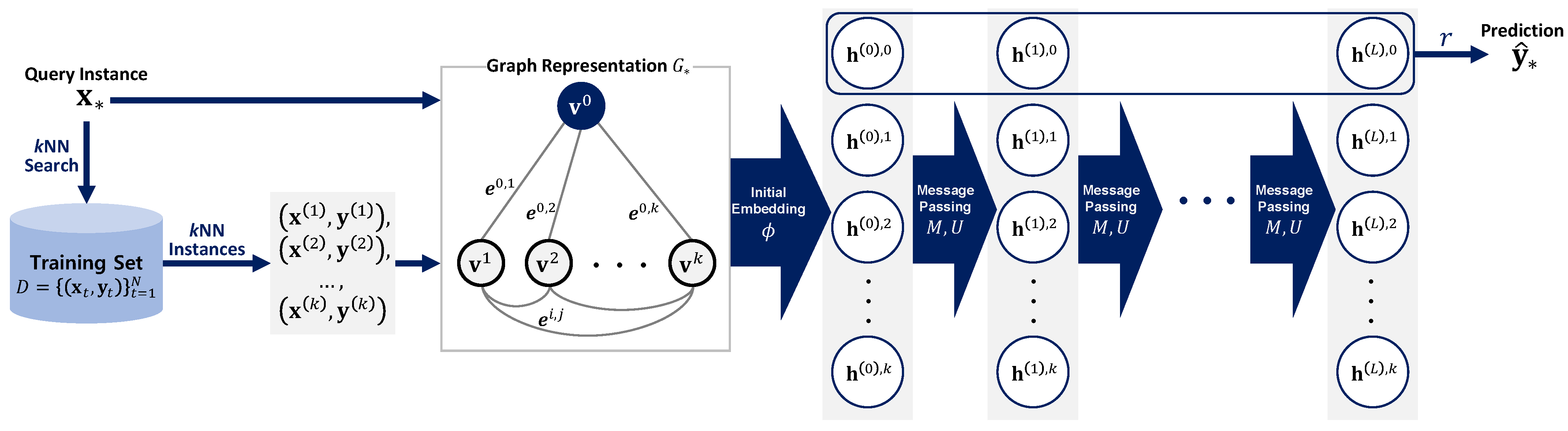
Once the prediction model f is trained, it can be used to predict unknown labels for new data. The prediction procedure is illustrated in Figure 1. Given a query instance ${\mathbf{x}}_{*}$ whose label ${\mathbf{y}}_{*}$ is unknown, its kNN instances $\mathcal{N}\left({\mathbf{x}}_{*}\right)={\left\{({\mathbf{x}}_{*}^{\left(i\right)},{\mathbf{y}}_{*}^{\left(i\right)})\right\}}_{i=1}^k$ are searched from the training dataset $\mathcal{D}$ based on the distance function d. Then, the corresponding graph ${\mathcal{G}}_{*}=g({\mathbf{x}}_{*};\mathcal{D})$ is generated. The prediction of ${\mathbf{y}}_{*}$, which is denoted by ${\widehat{\mathbf{y}}}_{*}$, is computed using the model f as:

$$\begin{array}{cc}\hfill {\widehat{\mathbf{y}}}_{*}& =f\left({\mathcal{G}}_{*}\right)=f\left(g({\mathbf{x}}_{*};\mathcal{D})\right).\hfill \end{array}$$

(7)

The proposed method does not require additional optimization procedures when making predictions. The prediction for a query instance is simply conducted by performing a kNN search to identify the kNN instances and then processing these instances with the model. This is advantageous in terms of computational efficiency.

As the proposed method learns the kNN rule, incremental learning can be implemented efficiently. This is the main advantage of the kNN algorithm compared to other learning algorithms, especially when additional training data are collected over time after the model is trained. When new labeled data are added to the training dataset $\mathcal{D}$, the prediction performance will be improved without updating the model.

4. Experimental Investigation

4.1. Datasets

The effectiveness of the proposed method was investigated through experiments on various benchmark datasets. They contained 20 classification datasets, and twenty regression datasets were collected from the UCI machine learning repository (http://archive.ics.uci.edu/ml/ (accessed on 10 January 2021) and the StatLib datasets archive (http://lib.stat.cmu.edu/datasets/(accessed on 10 January 2021)). The datasets used for classification tasks were annealing, balance, breastcancer, carevaluation, ecoli, glass, heart, ionosphere, iris, landcover, movement, parkinsons, seed, segment, sonar, vehicle, vowel, wine, yeast, and zoo. The datasets used for regression tasks were abalone, airfoil, appliances, autompg, bikesharing, bodyfat, cadata, concretecs, cpusmall, efficiency, housing, mg, motorcycle, newspopularity, skillcraft, spacega, superconductivity, telemonitoring, wine-red, and wine-white. Each dataset had a different number of instances with a different dimensionality. For each dataset, one-thousand instances were randomly sampled if the size of the dataset was greater than 1000. All numeric variables were normalized into the range of $[-1,1]$. The details of the datasets used are listed in

Table 1. Summary statistics of the error rate over different hyperparameter settings on the classification datasets.

Dataset [Size × Dim.]	No. of Classes	Uniform kNN			Weighted kNN			kNNGNN (Proposed)
		Average	Std. Dev.	Best	Average	Std. Dev.	Best	Average	Std. Dev.	Best
annealing [898 × 38]	5	0.0724	0.0356	0.0175	0.0364	0.0146	0.0174	0.0254	0.0046	0.0189
balance [625 × 4]	3	0.1453	0.0356	0.1130	0.1436	0.0377	0.1098	0.1327	0.0235	0.1046
breastcancer [683 × 9]	2	0.0382	0.0051	0.0306	0.0381	0.0051	0.0305	0.0369	0.0051	0.0290
carevaluation [1000 × 6]	4	0.2035	0.0306	0.1619	0.1858	0.0326	0.1461	0.1110	0.0354	0.0717
ecoli [336 × 7]	8	0.1853	0.0350	0.1427	0.1703	0.0256	0.1422	0.1849	0.0238	0.1555
glass [214 × 9]	6	0.3808	0.0425	0.3196	0.3441	0.0229	0.3074	0.3703	0.0259	0.3244
heart [298 × 13]	2	0.2081	0.0311	0.1792	0.2093	0.0349	0.1684	0.2126	0.0366	0.1804
ionosphere [351 × 34]	2	0.1808	0.0448	0.1120	0.1790	0.0428	0.1120	0.0838	0.0122	0.0681
iris [150 × 4]	3	0.0886	0.0522	0.0407	0.0766	0.0417	0.0427	0.0573	0.0157	0.0413
landcover [675 × 147]	9	0.3550	0.2050	0.1950	0.3450	0.2023	0.1847	0.2187	0.0513	0.1767
movement [360 × 90]	15	0.4808	0.1436	0.2125	0.3679	0.1125	0.2125	0.3300	0.0375	0.2569
parkinsons [195 × 22]	2	0.1634	0.0458	0.0775	0.1373	0.0368	0.0775	0.1536	0.0253	0.0918
seed [210 × 7]	3	0.0809	0.0114	0.0590	0.0779	0.0090	0.0610	0.0840	0.0078	0.0619
segment [1000 × 19]	7	0.1021	0.0281	0.0594	0.0840	0.0184	0.0586	0.0749	0.0079	0.0586
sonar [208 × 60]	2	0.2929	0.0621	0.1706	0.2684	0.0556	0.1706	0.2387	0.0349	0.1837
vehicle [846 × 18]	4	0.2951	0.0469	0.2276	0.2880	0.0432	0.2239	0.2775	0.0391	0.2191
vowel [990 × 10]	11	0.2868	0.1367	0.0516	0.1450	0.0553	0.0516	0.1504	0.0404	0.0561
wine [178 × 13]	3	0.1035	0.1010	0.0316	0.0861	0.0759	0.0304	0.0522	0.0329	0.0270
yeast [1000 × 8]	10	0.4495	0.0218	0.4305	0.4369	0.0292	0.4116	0.4514	0.0284	0.4222
zoo [101 × 16]	7	0.2269	0.1656	0.0505	0.1145	0.0776	0.0484	0.1012	0.0462	0.0709

The lowest values for each dataset are presented in bold.

and

Table 2. Summary statistics of the RMSE over different hyperparameter settings on the regression datasets.

Dataset [Size × Dim.]	Uniform kNN			Weighted kNN			kNNGNN (Proposed)
	Average	Std. Dev.	Best	Average	Std. Dev.	Best	Average	Std. Dev.	Best
abalone [1000 × 8]	0.2018	0.0183	0.1812	0.2006	0.0185	0.1804	0.1982	0.0103	0.1829
airfoil [1000 × 5]	0.2573	0.0185	0.2209	0.2270	0.0115	0.2060	0.1884	0.0125	0.1698
appliances [1000 × 25]	0.2663	0.0173	0.2533	0.2617	0.0190	0.2493	0.2601	0.0024	0.2563
autompg [392 × 7]	0.1846	0.0137	0.1642	0.1768	0.0139	0.1576	0.1821	0.0092	0.1715
bikesharing [1000 × 14]	0.1886	0.0315	0.1386	0.1813	0.0291	0.1348	0.0752	0.0481	0.0310
bodyfat [252 × 14]	0.1887	0.0345	0.1434	0.1855	0.0350	0.1416	0.1296	0.0459	0.0830
cadata [1000 × 8]	0.3384	0.0281	0.2999	0.3329	0.0285	0.2968	0.3153	0.0243	0.2848
concretecs [1000 × 8]	0.2566	0.0197	0.2237	0.2361	0.0197	0.2065	0.2036	0.0236	0.1804
cpusmall [1000 × 12]	0.1370	0.0503	0.0828	0.1247	0.0414	0.0810	0.0876	0.0143	0.0708
efficiency [768 × 8]	0.1468	0.0326	0.1077	0.1392	0.0346	0.0980	0.0700	0.0326	0.0483
housing [506 × 13]	0.2503	0.0197	0.2179	0.2333	0.0168	0.2038	0.2180	0.0199	0.1847
mg [1000 × 6]	0.2947	0.0249	0.2782	0.2891	0.0275	0.2697	0.2923	0.0181	0.2802
motorcycle [133 × 1]	0.2845	0.0473	0.2415	0.2862	0.0170	0.2730	0.2694	0.0195	0.2491
newspopularity [1000 × 58]	0.1242	0.0117	0.1156	0.1244	0.0117	0.1158	0.1218	0.0014	0.1200
skillcraft [1000 × 18]	0.3741	0.0435	0.3365	0.3734	0.0437	0.3354	0.3603	0.0241	0.3317
spacega [1000 × 6]	0.1576	0.0124	0.1415	0.1552	0.0131	0.1392	0.1556	0.0097	0.1421
superconductivity [1000 × 81]	0.2962	0.0449	0.2574	0.2790	0.0393	0.2454	0.2655	0.0105	0.2491
telemonitoring [1000 × 16]	0.4274	0.0363	0.3943	0.4235	0.0377	0.3905	0.4121	0.0125	0.3914
wine-red [1000 × 11]	0.2844	0.0234	0.2668	0.2751	0.0272	0.2547	0.2812	0.0088	0.2708
wine-white [1000 × 11]	0.2895	0.0232	0.2756	0.2832	0.0259	0.2671	0.2854	0.0077	0.2758

The lowest values for each dataset are presented in bold.

.

4.2. Compared Methods

Three kNN methods that use different weighting schemes w were compared in the experiments: uniform kNN, weighted kNN, and the proposed kNNGNN. The uniform kNN and weighted kNN respectively used the following weighting functions:

$$\begin{array}{cc}\hfill w_{\mathrm{U}}\left(d(\mathbf{x},{\mathbf{x}}^{\prime })\right)& =1/k;\hfill \\ \hfill w_{\mathrm{W}}\left(d(\mathbf{x},{\mathbf{x}}^{\prime })\right)& =1/d(\mathbf{x},{\mathbf{x}}^{\prime }).\hfill \end{array}$$

(8)

For kNNGNN, the weighting function is embedded implicitly.

For each method, the hyperparameter settings were varied to examine their effects. The candidates for the distance function d were as follows:

$$\begin{array}{cc}\hfill \mathrm{Manhattan}& d_{\mathrm{L}1}(\mathbf{x},{\mathbf{x}}^{\prime })=\left|\right|\mathbf{x}-{\mathbf{x}}^{\prime }{\left|\right|}_1;\hfill \\ \hfill \mathrm{Euclidean}& d_{\mathrm{L}2}(\mathbf{x},{\mathbf{x}}^{\prime })=\left|\right|\mathbf{x}-{\mathbf{x}}^{\prime }{\left|\right|}_2=\sqrt{{(\mathbf{x}-{\mathbf{x}}^{\prime })}^T(\mathbf{x}-{\mathbf{x}}^{\prime })};\hfill \\ \hfill \mathrm{Mahalanobis}& d_{\mathrm{M}}(\mathbf{x},{\mathbf{x}}^{\prime })=\sqrt{{(\mathbf{x}-{\mathbf{x}}^{\prime })}^T{S}^{-1}(\mathbf{x}-{\mathbf{x}}^{\prime })},\hfill \end{array}$$

(9)

where S is the covariance matrix of the input variables calculated from the training dataset.

Accordingly, there were a total of nine combinations of distance and weighting functions compared in the experiments, as summarized in

Table 3. Methods compared in the experiments.

		kNN Method (Weighting Function w)
		Uniform kNN	Weighted kNN	kNNGNN (Proposed)
distance function d	Manhattan (L1)	kNN_L1	WkNN_L1	kNNGNN_L1
	Euclidean (L2)	kNN_L2	WkNN_L2	kNNGNN_L2
	Mahalanobis (M)	kNN_M	WkNN_M	kNNGNN_M

. None of the methods used any additional optimization procedures when making predictions. For kNNGNN, the distance function was only explicitly used for the kNN search to generate graph representations of the data. For each combination, the effect of k was investigated on the prediction performance by varying its value from 1, 3, 5, 7, 10, 15, 20, and 30.

4.3. Experimental Settings

In the experiments, the performance of each method was evaluated using a two-fold cross-validation procedure. In this procedure, the original dataset was divided into five disjoint subsets. Then, two iterations were conducted, each of which used one subset and the other subset as the training and test sets, respectively. As performance measures, the misclassification error rate and root mean squared error (RMSE) were used for the classification and regression tasks, respectively. Given a test set denoted by ${\mathcal{D}}^{\prime }={\left\{({\mathbf{x}}_t,{\mathbf{y}}_t)\right\}}_{t=1}^{N^{\prime }}$, the performance measures are calculated as:

$$\begin{array}{cc}\hfill \mathrm{ErrorRate}=& \frac{1}{N^{\prime }}\sum _{({\mathbf{x}}_t,{\mathbf{y}}_t)\in {\mathcal{D}}^{\prime }}I(\mathtt{argmax}\left({\mathbf{y}}_t\right)\ne \mathtt{argmax}\left({\widehat{\mathbf{y}}}_t\right));\hfill \\ \hfill \mathrm{RMSE}=& \frac{1}{N^{\prime }}\sum _{({\mathbf{x}}_t,{\mathbf{y}}_t)\in {\mathcal{D}}^{\prime }}{({\mathbf{y}}_t-{\widehat{\mathbf{y}}}_t)}^2.\hfill \end{array}$$

(10)

For the proposed method, each prediction model was built based on the following configurations. In the objective function $\mathcal{J}$, the loss function $\mathcal{L}$ used for the classification and regression tasks was set to cross-entropy and squared error, respectively. For the model, the hyperparameter L was set to 3, as Gilmer et al. [32] demonstrated any $L\ge 3$ would work. The hyperparameter p was explored on $\{10,20,50\}$ by holdout validation. In the training phase, dropout was applied to the function r with a dropout rate of 0.1 for regularization [34]. During the training, eighty percent and 20% of the training set were used to train and validate the model, respectively. The model parameters were updated using the Adam optimizer with a batch size of 20. The learning rate was set to 10${}^{-3}$ at the first training epoch and was reduced by a factor of 0.1 if no improvement in the validation loss was observed for 10 consecutive epochs. The training was terminated when the learning rate was decreased to 10${}^{-7}$ or the number of epochs reached 500. In the inference phase, for each query instance, thirty different outputs were obtained by performing stochastic forward passes through the trained model with the dropout turned on [35]. The average of these outputs was then used to obtain the predicted label for the instance.

All baseline methods were implemented using the scikit-learn package in Python. The proposed method was implemented based on GPU-accelerated TensorFlow in Python. All experiments were performed 10 times independently with different random seeds. For the results, the average performance over the repetitions was compared. Then, for each of the three weighting functions w, the summary statistics of the performance over different settings of distance functions d and the number of neighbors k are reported.

4.4. Results and Discussion

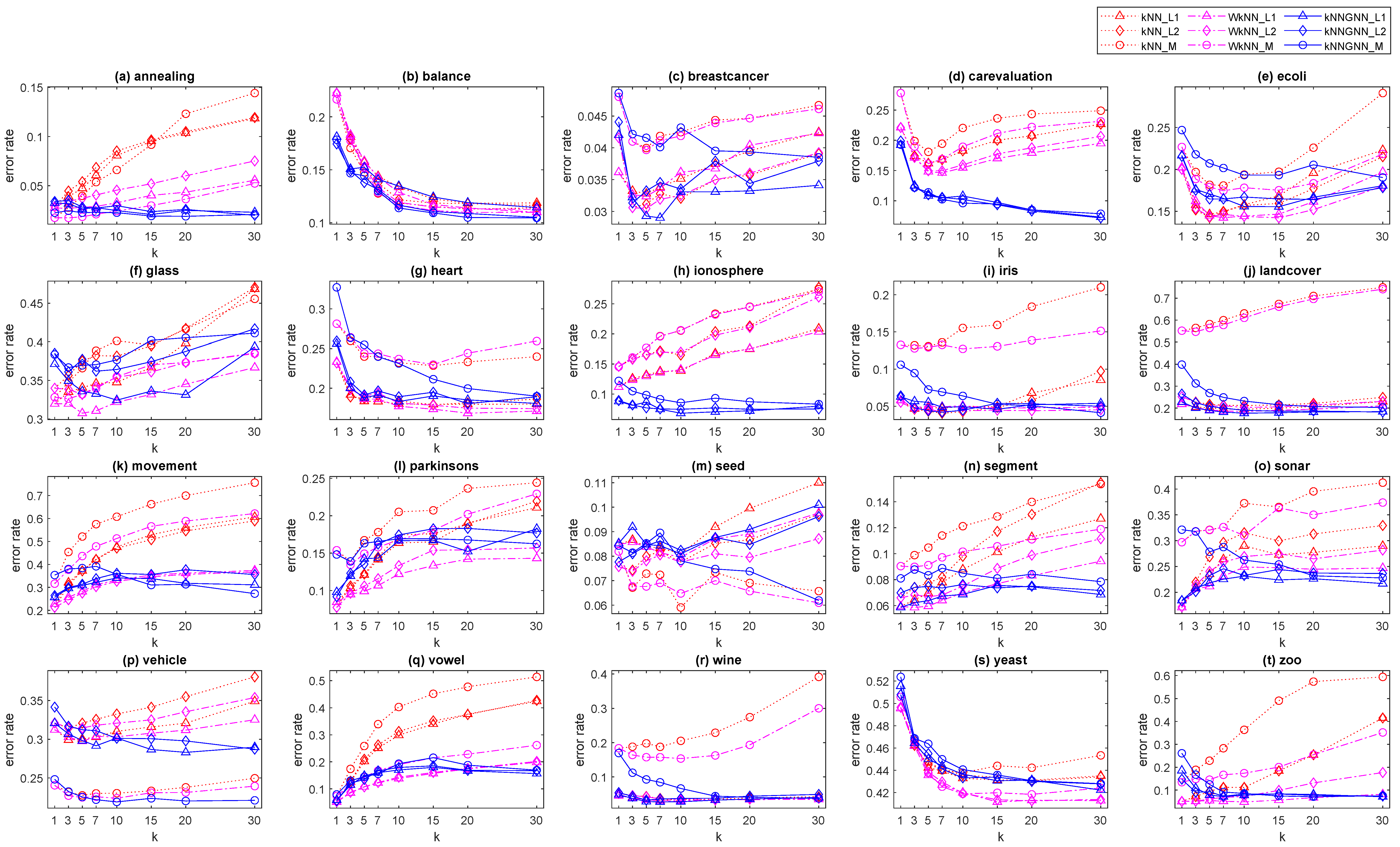
Figure 2 shows the error rate comparison results of the baseline and proposed methods with varying the hyperparameter settings on 20 classification datasets. Compared to the baseline methods, kNNGNN overall yielded lower error rates at various values of k for most datasets. For the results with different hyperparameters, the average, standard deviation, and best error rate for each dataset are summarized in Table 1. kNNGNN yielded the lowest average and standard deviation of the error rate over different hyperparameters on most datasets, which indicated that the performance of kNNGNN was less sensitive to its hyperparameter settings. In particular, kNNGNN was superior to the baseline method when the hyperparameter k was larger.

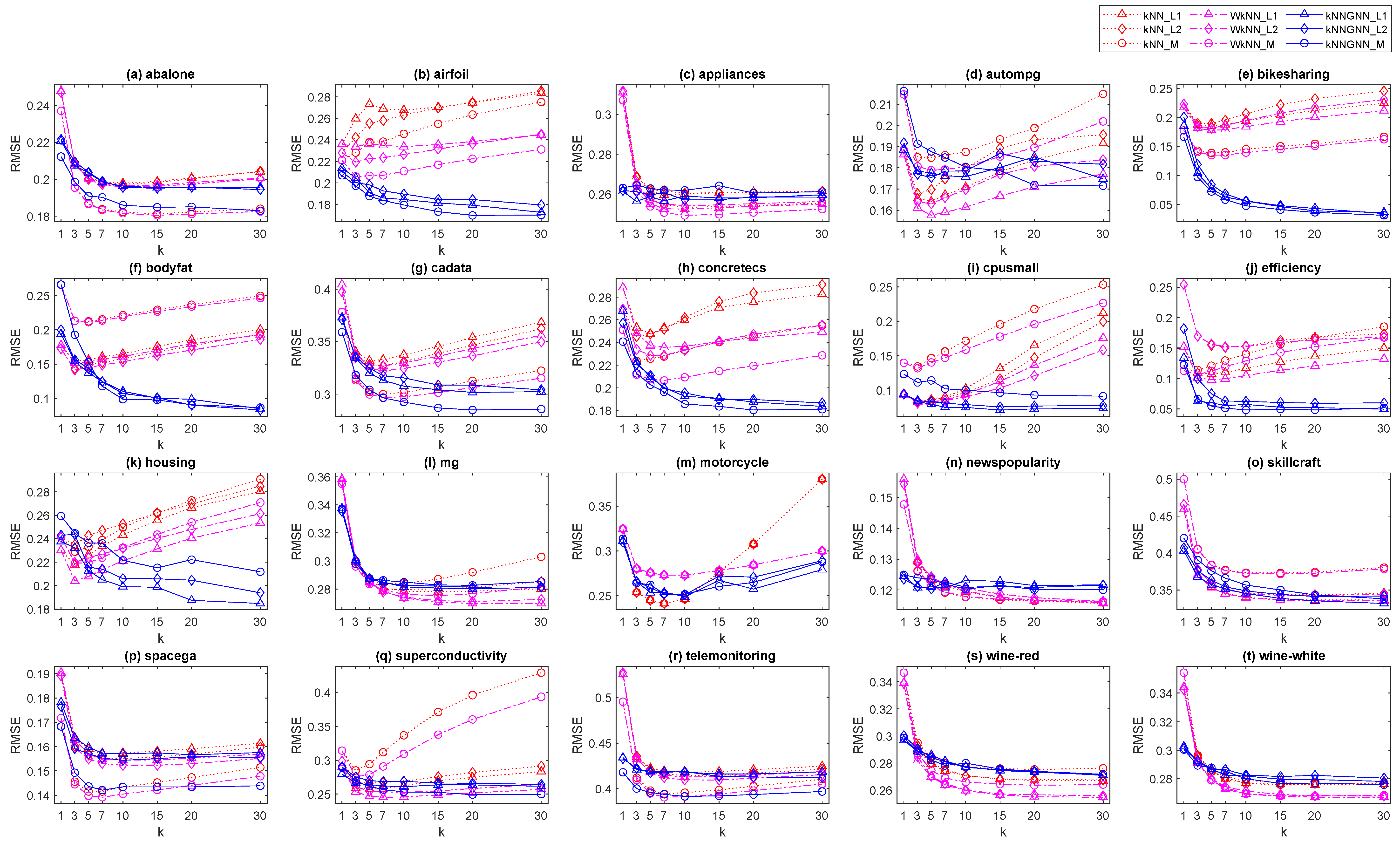
Figure 3 compares the baseline and proposed methods in terms of the RMSE with varying hyperparameter settings on 20 regression datasets. As shown in this figure, the performance curves of kNNGNN flattened as k increased on most datasets, whereas the RMSE of the baseline methods tended to increase at large k for some datasets. Table 2 shows the average, standard deviation, and best RMSE for different hyperparameter settings for each dataset. The behavior of kNNGNN was similar to that of the classification tasks. kNNGNN showed stable performance against changes in the hyperparameter settings. kNNGNN yielded the lowest average and standard deviation of the RMSE for the majority of datasets.

In summary, the experimental results successfully demonstrated the effectiveness of kNNGNN in improving the prediction performance for both classification and regression tasks. Although kNNGNN failed to yield the lowest error for some datasets, kNNGNN yielded high robustness to its hyperparameters. This indicated that kNNGNN would provide comparable performance without carefully tuning its hyperparameters; thus, it can be preferred in practice considering the difficulty of choosing the optimal hyperparameter setting. Because the performance curve of kNNGNN flattened at large k values on most datasets, setting a moderate k value around 15∼20 would be reasonable considering the trade-off between the performance and computational cost.

5. Conclusions

This study presented kNNGNN, which learns a task-specific kNN rule from data in an end-to-end fashion. The proposed method constructed the kNN rule in the form of a graph neural network, in which the distance and weighting functions were embedded implicitly. The graph neural network considered the kNN graph of an instance as the input to predict the label of the instance. Owing to the flexibility of neural networks, the method can be applied to any form of supervised learning tasks including classification and regression. It does not require any extra optimization procedure when making predictions for new data, which is beneficial in terms of computational efficiency. Moreover, as the method learns the kNN rule instead of the explicit relationship between the input and output variables, incremental learning can be implemented efficiently.

The effectiveness of the proposed method was demonstrated through experiments on benchmark classification and regression datasets. The results showed that the proposed method can yield comparable prediction performance with less sensitivity to the choice of its hyperparameters. The proposed method allows more robust kNN learning without carefully tuning the hyperparameters. The use of a graph neural network for kNN learning may still have room for improvement and thus merits further investigation. One practical concern is the high complexity of a graph neural network in terms of time and space, which increases with k. A graph neural network cannot be trained in a reasonable amount of time without using a GPU. Alleviation of complexity to improve learning efficiency will be an avenue for future work.

References

- Wu, X.; Kumar, V.; Quinlan, J.R.; Ghosh, J.; Yang, Q.; Motoda, H.; McLachlan, G.J.; Ng, A.; Liu, B.; Philip, S.Y.; et al. Top 10 algorithms in data mining. Knowl. Inf. Syst. 2008, 14, 1–37. [Google Scholar] [CrossRef] [Green Version]
- Cover, T.; Hart, P. Nearest neighbor pattern classification. IEEE Trans. Inf. Theory 1967, 13, 21–27. [Google Scholar] [CrossRef]
- Jiang, L.; Cai, Z.; Wang, D.; Jiang, S. Survey of improving k-nearest-neighbor for classification. In Proceedings of the International Conference on Fuzzy Systems and Knowledge Discovery, Haikou, China, 24–27 August 2007; pp. 679–683. [Google Scholar]
- Atkeson, C.G.; Moore, A.W.; Schaal, S. Locally Weighted Learning. Artif. Intell. Rev. 1997, 11, 11–73. [Google Scholar] [CrossRef]
- Wolpert, D.H. The lack of a priori distinctions between learning algorithms. Neural Comput. 1996, 8, 1341–1390. [Google Scholar] [CrossRef]
- Bergstra, J.; Bengio, Y. Random search for hyper-parameter optimization. J. Mach. Learn. Res. 2012, 13, 281–305. [Google Scholar]
- Snoek, J.; Larochelle, H.; Adams, R.P. Practical Bayesian optimization of machine learning algorithms. In Proceedings of the Advances in Neural Information Processing Systems, Lake Tahoe, NV, USA, 3–6 December 2012; pp. 2951–2959. [Google Scholar]
- Zhang, S.; Li, X.; Zong, M.; Zhu, X.; Wang, R. Efficient kNN classification with different numbers of nearest neighbors. IEEE Trans. Neural Netw. Learn. Syst. 2017, 29, 1774–1785. [Google Scholar] [CrossRef] [PubMed]
- Zhang, S.; Cheng, D.; Deng, Z.; Zong, M.; Deng, X. A novel kNN algorithm with data-driven k parameter computation. Pattern Recognit. Lett. 2018, 109, 44–54. [Google Scholar] [CrossRef]
- Wang, J.; Neskovic, P.; Cooper, L.N. Neighborhood size selection in the k-nearest-neighbor rule using statistical confidence. Pattern Recognit. 2006, 39, 417–423. [Google Scholar] [CrossRef]
- García-Pedrajas, N.; del Castillo, J.A.R.; Cerruela-García, G. A proposal for local k values for k-nearest neighbor rule. IEEE Trans. Neural Netw. Learn. Syst. 2015, 28, 470–475. [Google Scholar] [CrossRef]
- Zhang, S.; Li, X.; Zong, M.; Zhu, X.; Cheng, D. Learning k for kNN classification. ACM Trans. Intell. Syst. Technol. 2017, 8, 43. [Google Scholar] [CrossRef] [Green Version]
- Li, D.; Tian, Y. Survey and experimental study on metric learning methods. Neural Netw. 2018, 105, 447–462. [Google Scholar] [CrossRef]
- Kulis, B. Metric Learning: A Survey. Found. Trends Mach. Learn. 2013, 5, 287–364. [Google Scholar] [CrossRef]
- Weinberger, K.Q.; Saul, L.K. Distance metric learning for large margin nearest neighbor classification. J. Mach. Learn. Res. 2009, 10, 207–244. [Google Scholar]
- Goldberger, J.; Roweis, S.; Hinton, G.; Salakhutdinov, R. Neighbourhood components analysis. In Advances in Neural Information Processing Systems; MIT Press: Cambridge, MA, USA, 2004; pp. 513–520. [Google Scholar]
- Sugiyama, M. Dimensionality reduction of multimodal labeled data by local fisher discriminant analysis. J. Mach. Learn. Res. 2007, 8, 1027–1061. [Google Scholar]
- Davis, J.V.; Kulis, B.; Jain, P.; Sra, S.; Dhillon, I.S. Information-theoretic metric learning. In Proceedings of the International Conference on Machine Learning, Cincinnati, OH, USA, 13–15 December 2007; pp. 209–216. [Google Scholar]
- Wang, W.; Hu, B.G.; Wang, Z.F. Globality and locality incorporation in distance metric learning. Neurocomputing 2014, 129, 185–198. [Google Scholar] [CrossRef]
- Assi, K.C.; Labelle, H.; Cheriet, F. Modified large margin nearest neighbor metric learning for regression. IEEE Signal Process. Lett. 2014, 21, 292–296. [Google Scholar] [CrossRef] [Green Version]
- Weinberger, K.Q.; Tesauro, G. Metric Learning for Kernel Regression. In Proceedings of the International Conference on Artificial Intelligence and Statistics, San Juan, Puerto Rico, 21–24 March 2007; pp. 612–619. [Google Scholar]
- Nguyen, B.; Morell, C.; De Baets, B. Large-scale distance metric learning for k-nearest neighbors regression. Neurocomputing 2016, 214, 805–814. [Google Scholar] [CrossRef]
- Wang, J.; Neskovic, P.; Cooper, L.N. Improving nearest neighbor rule with a simple adaptive distance measure. Pattern Recognit. Lett. 2007, 28, 207–213. [Google Scholar] [CrossRef]
- Zhou, C.Y.; Chen, Y.Q. Improving nearest neighbor classification with cam weighted distance. Pattern Recognit. 2006, 39, 635–645. [Google Scholar] [CrossRef]
- Jahromi, M.Z.; Parvinnia, E.; John, R. A method of learning weighted similarity function to improve the performance of nearest neighbor. Inf. Sci. 2009, 179, 2964–2973. [Google Scholar] [CrossRef]
- Paredes, R.; Vidal, E. Learning weighted metrics to minimize nearest-neighbor classification error. IEEE Trans. Pattern Anal. Mach. Intell. 2006, 28, 1100–1110. [Google Scholar] [CrossRef] [PubMed]
- Domeniconi, C.; Peng, J.; Gunopulos, D. Locally adaptive metric nearest-neighbor classification. IEEE Trans. Pattern Anal. Mach. Intell. 2002, 24, 1281–1285. [Google Scholar] [CrossRef] [Green Version]
- Kang, P.; Cho, S. Locally linear reconstruction for instance-based learning. Pattern Recognit. 2008, 41, 3507–3518. [Google Scholar] [CrossRef]
- Keller, J.M.; Gray, M.R.; Givens, J.A. A fuzzy k-nearest neighbor algorithm. IEEE Trans. Syst. Man, Cybern. 1985, SMC-15, 580–585. [Google Scholar] [CrossRef]
- Biswas, N.; Chakraborty, S.; Mullick, S.S.; Das, S. A parameter independent fuzzy weighted k-nearest neighbor classifier. Pattern Recognit. Lett. 2018, 101, 80–87. [Google Scholar] [CrossRef]
- Maillo, J.; García, S.; Luengo, J.; Herrera, F.; Triguero, I. Fast and scalable approaches to accelerate the fuzzy k-Nearest neighbors classifier for big data. IEEE Trans. Fuzzy Syst. 2019, 28, 874–886. [Google Scholar] [CrossRef]
- Gilmer, J.; Schoenholz, S.S.; Riley, P.F.; Vinyals, O.; Dahl, G.E. Neural message passing for quantum chemistry. In Proceedings of the International Conference on Machine Learning, Sydney, Australia, 11–15 August 2017; pp. 1263–1272. [Google Scholar]
- Cho, K.; Van Merriënboer, B.; Gulcehre, C.; Bahdanau, D.; Bougares, F.; Schwenk, H.; Bengio, Y. Learning phrase representations using RNN encoder-decoder for statistical machine translation. In Proceedings of the Conference on Empirical Methods in Natural Language Processing, Doha, Qatar, 25–29 October 2014; pp. 1724–1734. [Google Scholar]
- Srivastava, N.; Hinton, G.; Krizhevsky, A.; Sutskever, I.; Salakhutdinov, R. Dropout: A simple way to prevent neural networks from overfitting. J. Mach. Learn. Res. 2014, 15, 1929–1958. [Google Scholar]
- Gal, Y.; Ghahramani, Z. Dropout as a Bayesian approximation: Representing model uncertainty in deep learning. In Proceedings of the International Conference on Machine Learning, New York, NY, USA, 19–24 June 2016; pp. 1050–1059. [Google Scholar]
Figure 1.
Schematic of the kNN graph neural network (kNNGNN) prediction procedure.
Figure 2.
Error rate comparison with varying hyperparameter settings on classification datasets.
Figure 3.
RMSE comparison with varying hyperparameters on regression datasets.