An Efficient and Accurate Method for the Conservative Swift–Hohenberg Equation and Its Numerical Implementation

Department of Mathematics, Kwangwoon University, Seoul 01897, Korea
Mathematics 2020, 8(9), 1502; https://doi.org/10.3390/math8091502
Submission received: 21 August 2020
/
Revised: 30 August 2020
/
Accepted: 2 September 2020
/
Published: 4 September 2020
(This article belongs to the Special Issue Open Source Codes for Numerical Analysis)
Abstract
:The conservative Swift–Hohenberg equation was introduced to reformulate the phase-field crystal model. A challenge in solving the conservative Swift–Hohenberg equation numerically is how to treat the nonlinear term to preserve mass conservation without compromising efficiency and accuracy. To resolve this problem, we present a linear, high-order, and mass conservative method by placing the linear and nonlinear terms in the implicit and explicit parts, respectively, and employing the implicit-explicit Runge–Kutta method. We show analytically that the method inherits the mass conservation. Numerical experiments are presented demonstrating the efficiency and accuracy of the proposed method. In particular, long time simulation for pattern formation in 2D is carried out, where the phase diagram can be observed clearly. The MATLAB code for numerical implementation of the proposed method is provided in Appendix.
1. Introduction
The phase-field crystal (PFC) model describes the microstructure of two-phase systems on atomic length and diffusive time scales and has been used to study grain growth, dendritic and eutectic solidification, and epitaxial growth [1,2]. The PFC model is the -gradient flow for the Swift–Hohenberg (SH) energy functional [3]:
where is a domain in , is the density field, , and and are positive constants with physical significance.
Recently, conservative SH equations were introduced to reformulate the PFC model [4,5]. In [4], Zhang and Yang derived the following equation:
where is a nonlocal Lagrange multiplier and , and developed a second-order energy stable scheme by combining the invariant energy quadratization idea with the stabilization technique. However, the scheme involves solving a linear system with complicated variable coefficients. In [5], Lee introduced the following equation:
where is a nonlocal and local Lagrange multiplier and , and proposed mass conservative first- and second-order operator splitting methods. However, the methods lead to the necessity nonlinear equations to be solved at each time step thus require an iterative solver for solving the nonlinear equations.
Therefore, the aim of this paper is to present an efficient and accurate method that preserves mass conservation for solving the conservative SH Equation (3). We place the linear and nonlinear terms in the implicit and explicit parts, respectively, where an extra linear stabilizing term is added to improve the stability while preserving the simplicity. And we employ the implicit-explicit Runge–Kutta (RK) method [6]. As a result, our method is linear, high-order accurate in time, and mass conservative. We show analytically that the method inherits the mass conservation. In addition, the Fourier spectral method [5,7,8,9,10] is used for the spatial discretization. The MATLAB code for numerical implementation of the method in 2D is provided in Appendix A.
This paper is organized as follows. In Section 2, we construct the linear, high-order, and mass conservative method and show analytically that the method inherits the mass conservation. Numerical examples showing the efficiency and accuracy of the proposed method are presented in Section 3. Finally, conclusions are drawn in Section 4. In Appendix A, we provide the MATLAB code for numerical implementation of the proposed method in 2D.
2. Linear, High-Order, and Mass Conservative Method
For simplicity and clarity of exposition, we consider Equation (3) in one-dimensional space with a periodic boundary condition:
where . Two- and three-dimensional cases are defined analogously. Let M be a positive integer, be the space step size, and be the time step size. Let be an approximation of , where for and . The discrete Fourier transform and its inverse transform are
and
where .
To develop a linear, high-order (up to third-order), and mass conservative method for solving Equation (4), we treat implicitly and explicitly, where s is a non-negative number, and employ the implicit-explicit RK method. First- (S1), second- (S2), and third- (S3) order methods are as follows:
where , , , , and .
For the method S1, Equation (7) can be transformed into the discrete Fourier space using (6):
where and denotes the discrete Fourier transform. After updating with , we recover from using (6). To satisfy the mass conservation property, we should have for . From Equation (14), we get
since
Thus, the method S1 inherits the mass conservation. Next, for the method S2, we have
from Equation (8) and
from Equation (9). For the method S3, we have from Equations (10)–(12) and
from Equation (13). Thus, the methods S2 and S3 also inherit the mass conservation.
3. Numerical Experiments
3.1. Convergence Test
We demonstrate the convergence of the proposed methods with the initial condition [11,12]
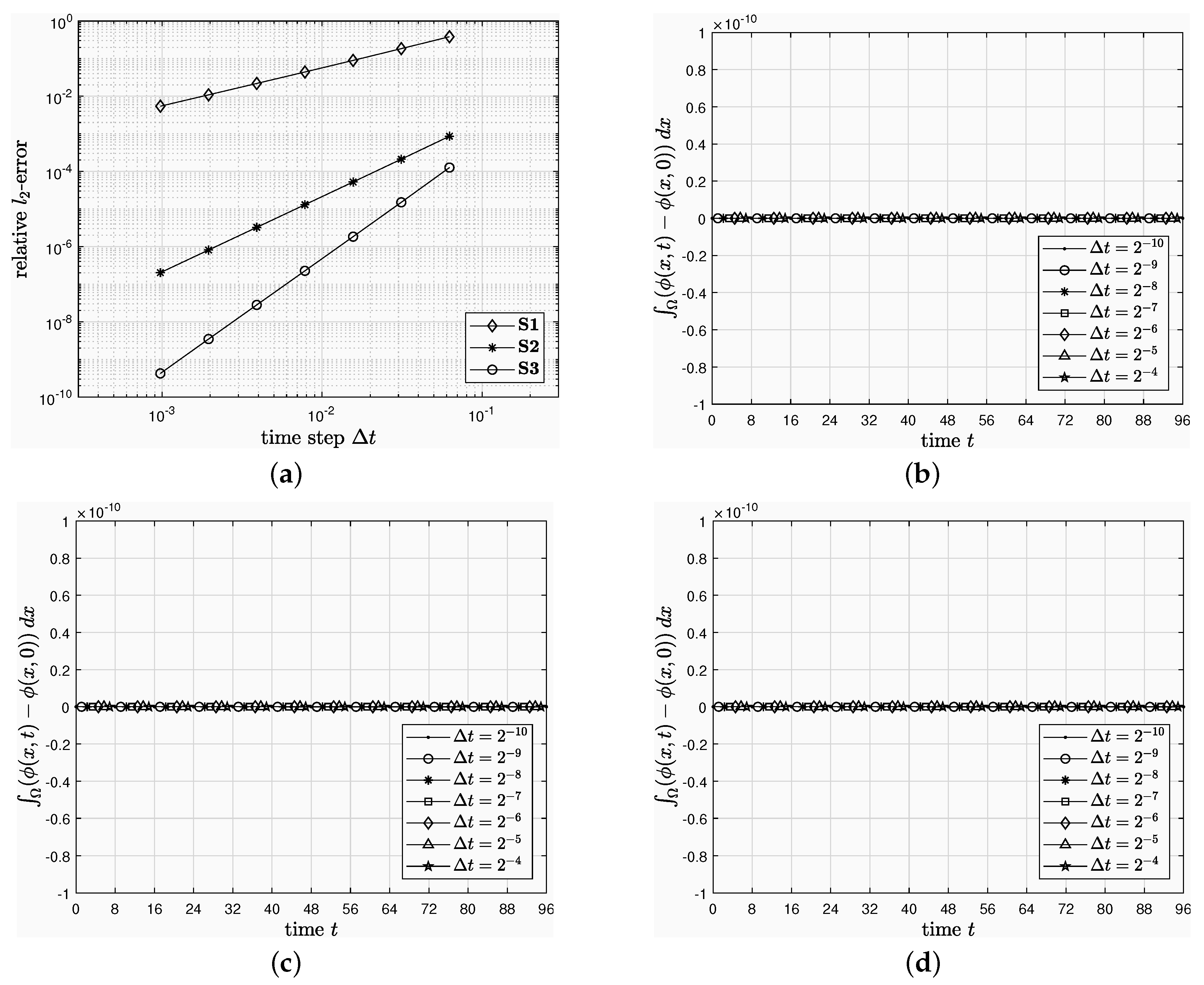
on . We set , , , and , and compute for . The grid size is fixed to which provides enough spatial accuracy. To estimate the convergence rate with respect to , simulations are performed by varying . We take the quadruply over-resolved numerical solution using the method S3 as the reference solution. Figure 1a shows the relative -errors of for various time steps. Here, the errors are computed by comparison with the reference solution. In addition, Figure 1b–d show the evolution of using the methods S1–S3, respectively. Here, is approximated by . It is observed that the methods give desired order of accuracy in time and conserve the total mass.
3.2. Efficiency of the Proposed Method
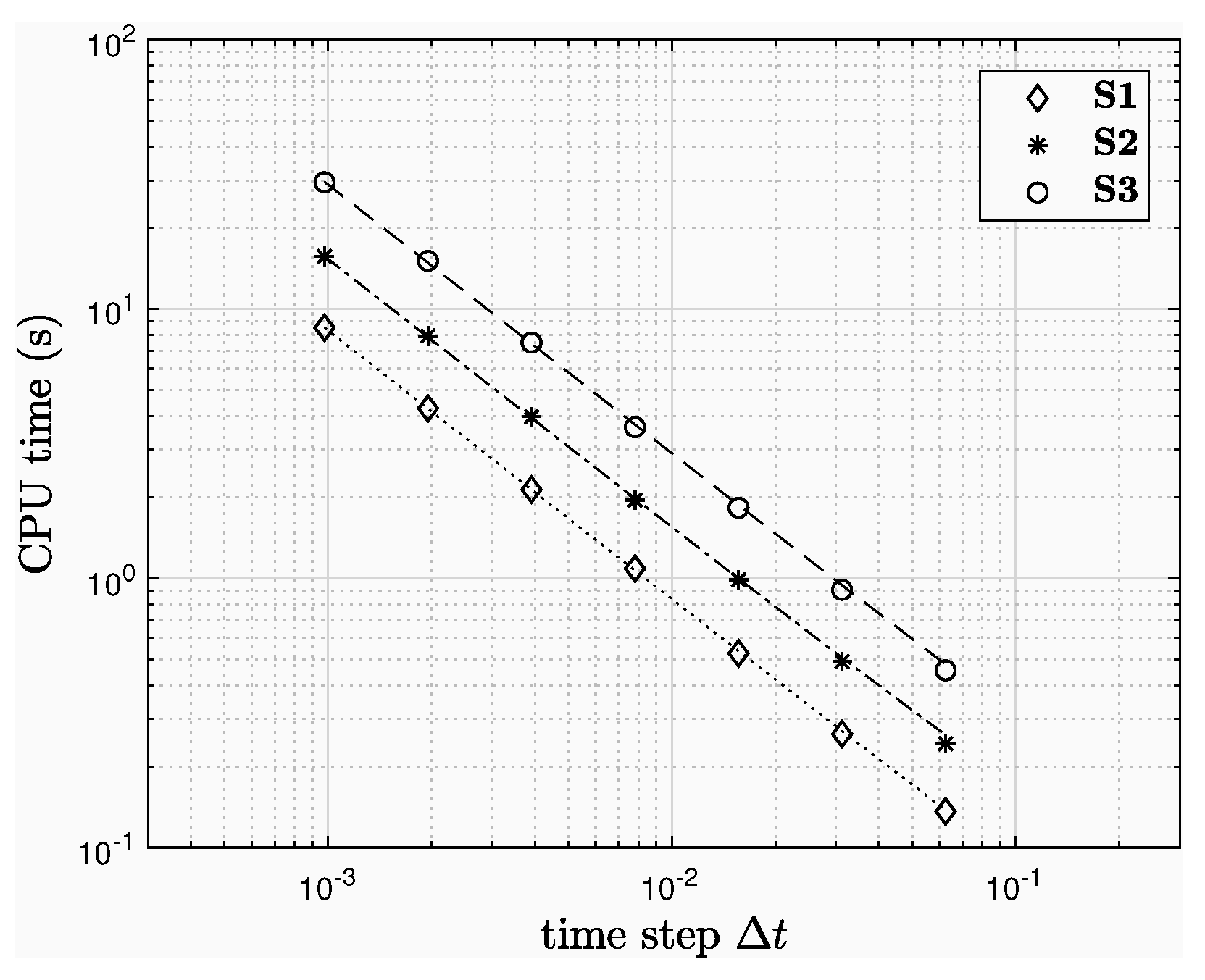
To show the efficiency of the proposed method, we take the initial condition (20) and parameter values used to create Figure 1. Figure 2 presents the CPU time (in seconds, averaged over 10 trials performed on Intel Core i5-7500 CPU at 3.40 GHz with 8 GB RAM) consumed using the methods S1–S3 for various time steps. The results suggest that the CPU time is almost linear with respect to the number of steps and the methods S2 and S3 are about two and four times more expensive than the method S1, respectively.
3.3. Phase Diagram in 2D
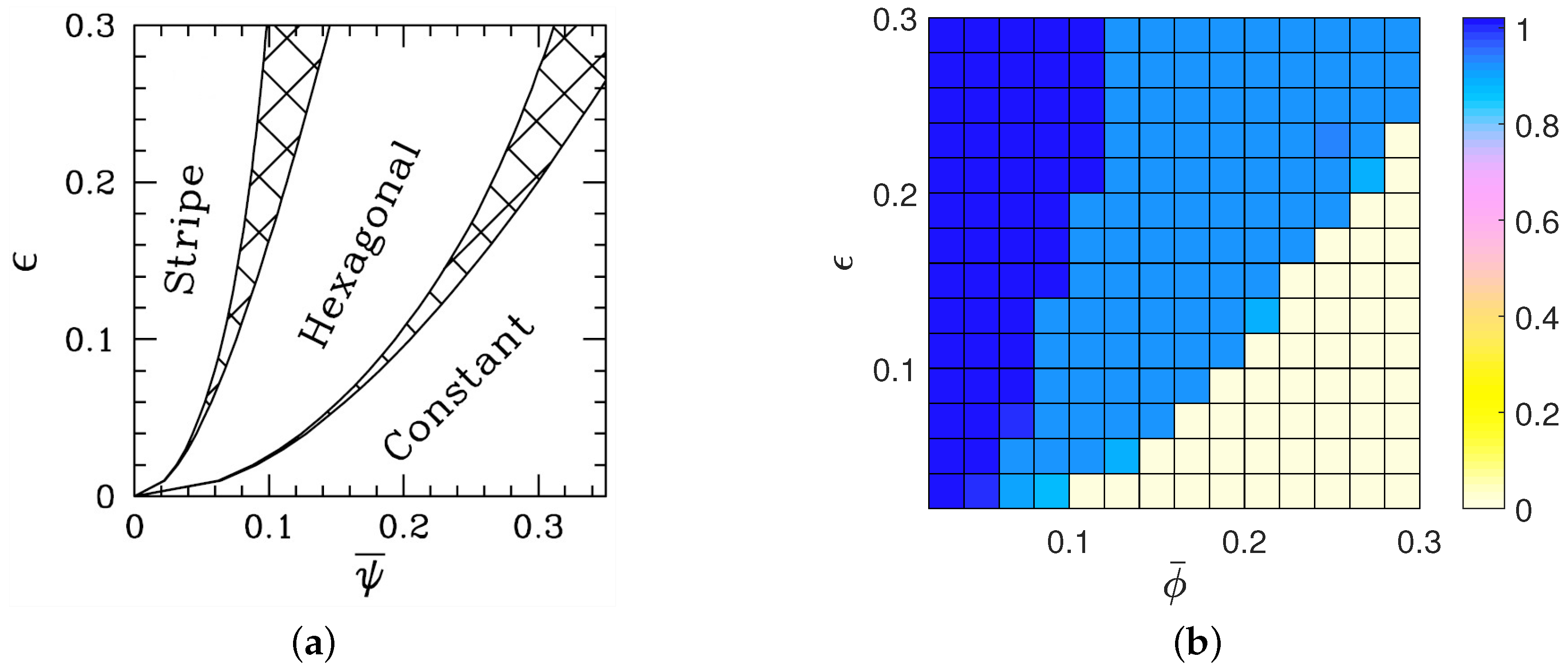
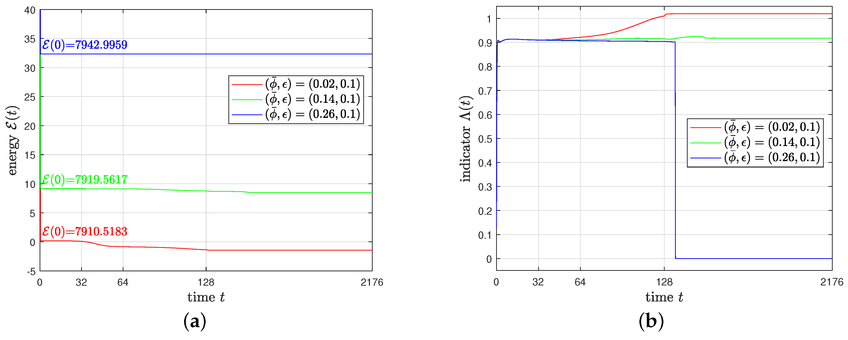
In 2D, the phase diagram contains striped, hexagonal, and constant states depending on the values of and [1] (see Figure 3a). To verify that the proposed method does lead to the expected states, we take an initial condition as on . Here, rand is a random number between and at the grid points, and we use , , , , and the method S3. For saving computational time, we choose different time steps as the solution evolves from random noisy stage to smooth stage: for and for . To estimate the phase diagram numerically, we calculate the indicator function defined similarly in [13]:
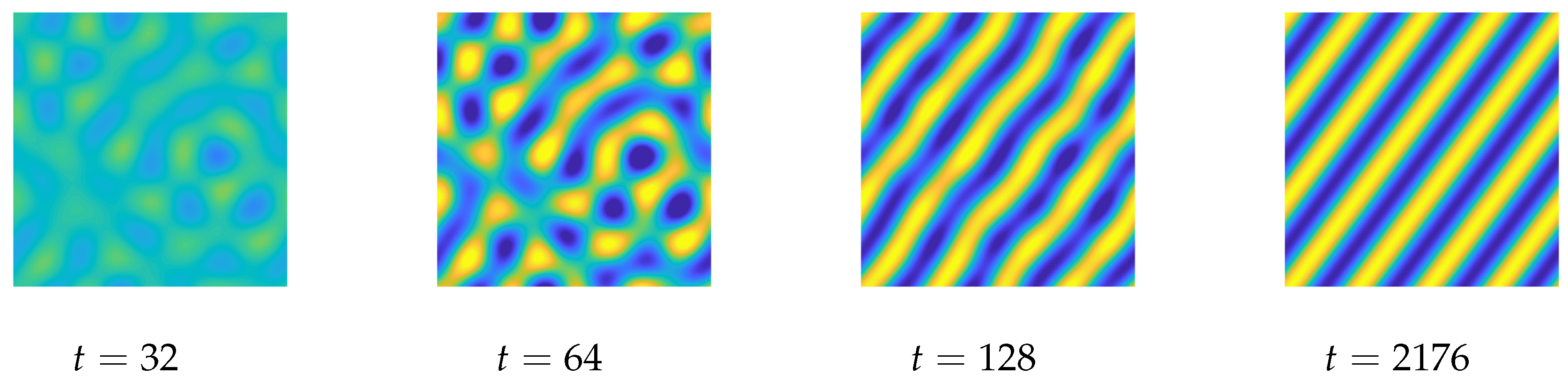
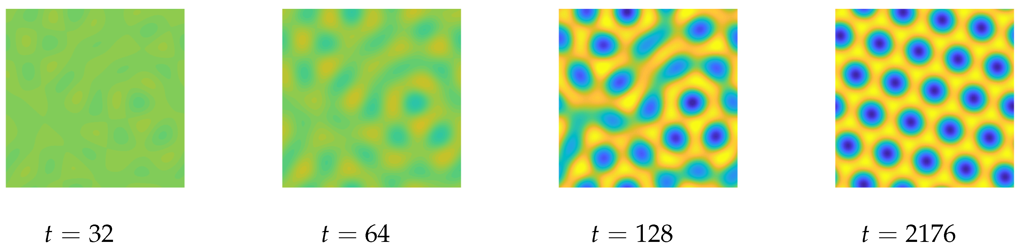
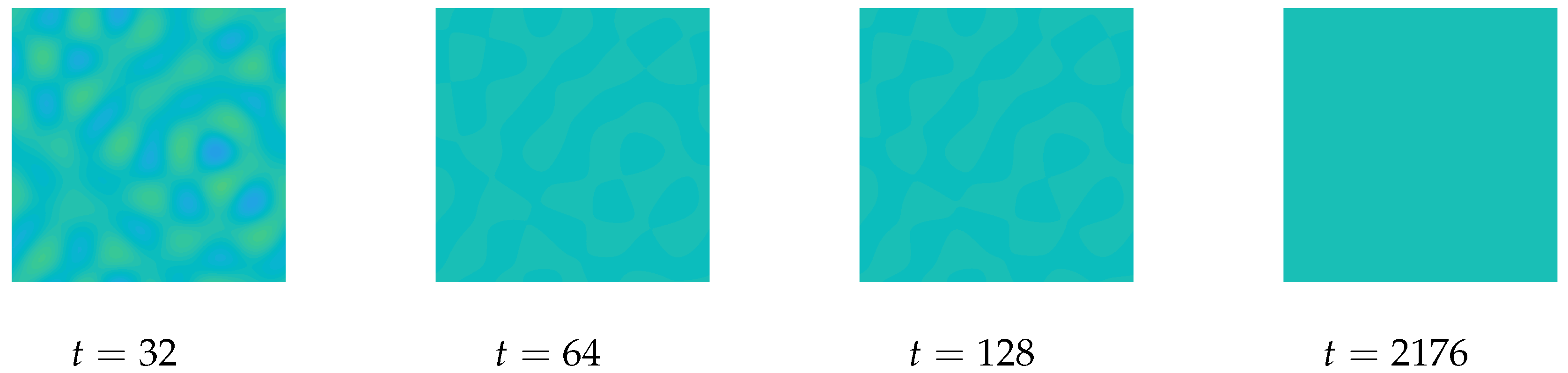
Here, we set if is less than . Figure 3b shows at with various and . Results in Figure 3b are consistent with the phase diagram in Figure 3a. Sample time evolutions of with , , and are shown in Figure 4, Figure 5 and Figure 6, respectively. Figure 7 shows evolutions of and with used in Figure 4, Figure 5 and Figure 6. We remark that the solution with has a small but measurable perturbation from a constant state until (see Figure 6). In this case, and is calculated using . Afterward, the solution evolves to a constant state, i.e., and . Thus, is calculated using and approximately zero.
3.4. Comparison with Other Method
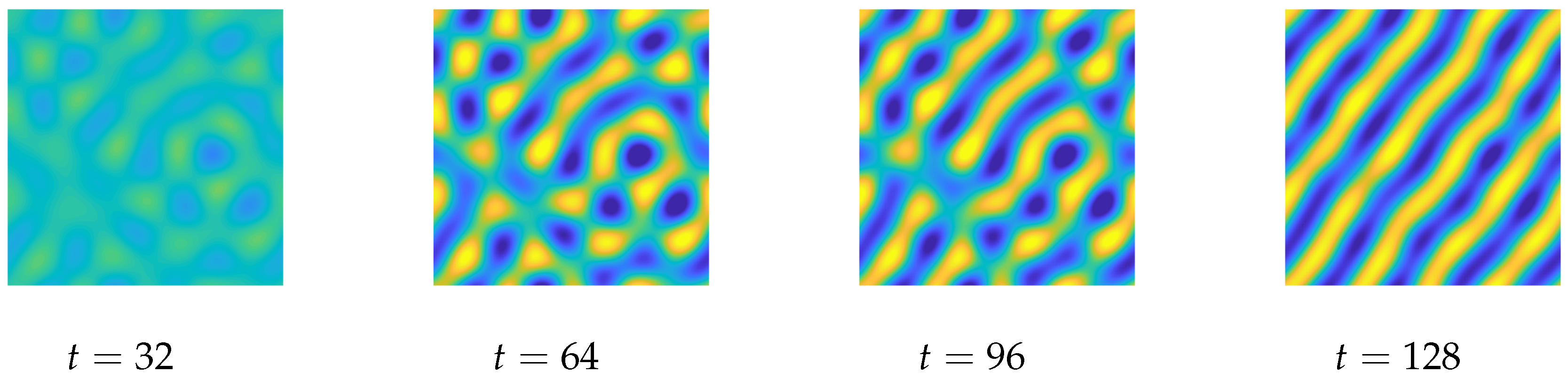
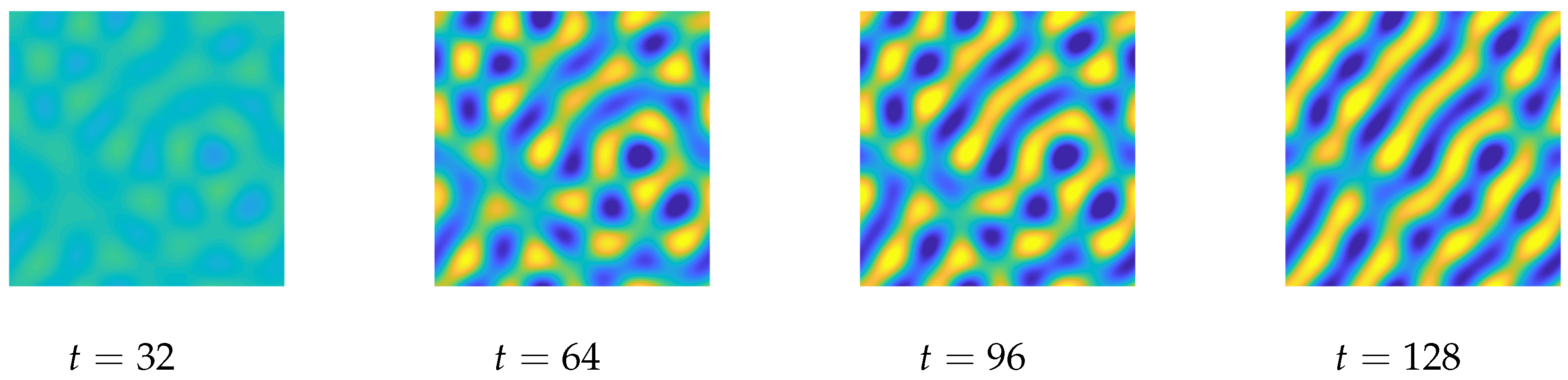
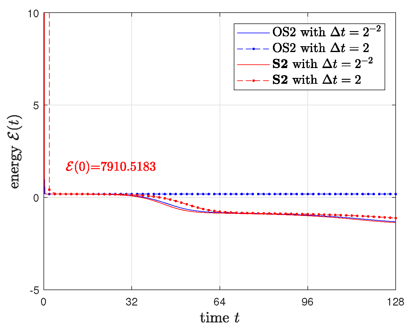
To compare the proposed method with other method, we solve the conservative SH Equation (3) using the proposed method S2 and the second-order operator splitting (OS2) method in [5] with the initial condition and parameter values used to create Figure 4 except for . Figure 8 and Figure 9 show evolutions of using the method OS2 with and 2, respectively. The method OS2 with a smaller time step leads to the expected striped state, whereas a constant state is observed for . Figure 10 and Figure 11 show evolutions of using the method S2 with and 2, respectively. The method S2 gives the striped state even for a large time step. Evolutions of for Figure 8, Figure 9, Figure 10 and Figure 11 are shown in Figure 12.
4. Conclusions
In this paper, we developed linear, first-, second-, and third-order, and mass conservative methods for the conservative SH equation by placing the linear and nonlinear terms in the implicit and explicit parts, respectively, and employing the implicit-explicit RK method. We confirmed that the proposed methods give desired order of accuracy in time, inherit the mass conservation, and are efficient (the CPU time was almost linear with respect to the number of steps and of stages). And we performed long time simulation for pattern formation in 2D, where the phase diagram can be observed clearly.
Funding
This work was supported by the National Research Foundation of Korea (NRF) grant funded by the Korea government (MSIT) (No. 2019R1C1C1011112).
Acknowledgments
The corresponding author thanks the reviewers for the constructive and helpful comments on the revision of this article
Conflicts of Interest
The author declares no conflict of interest.
Appendix A. Matlab Code


References
- Elder, K.R.; Katakowski, M.; Haataja, M.; Grant, M. Modeling elasticity in crystal growth. Phys. Rev. Lett. 2002, 88, 245701. [Google Scholar] [CrossRef] [Green Version]
- Elder, K.R.; Grant, M. Modeling elastic and plastic deformations in nonequilibrium processing using phase field crystals. Phys. Rev. E 2004, 70, 051605. [Google Scholar] [CrossRef] [PubMed] [Green Version]
- Swift, J.; Hohenberg, P.C. Hydrodynamic fluctuations at the convective instability. Phys. Rev. A 1977, 15, 319–328. [Google Scholar] [CrossRef] [Green Version]
- Zhang, J.; Yang, X. Numerical approximations for a new L2-gradient flow based Phase field crystal model with precise nonlocal mass conservation. Comput. Phys. Commun. 2019, 243, 51–67. [Google Scholar] [CrossRef]
- Lee, H.G. A new conservative Swift-Hohenberg equation and its mass conservative method. J. Comput. Appl. Math. 2020, 375, 112815. [Google Scholar] [CrossRef]
- Ascher, U.M.; Ruuth, S.J.; Spiteri, R.J. Implicit-explicit Runge-Kutta methods for time-dependent partial differential equations. Appl. Numer. Math. 1997, 25, 151–167. [Google Scholar] [CrossRef]
- Lee, H.G. A semi-analytical Fourier spectral method for the Swift-Hohenberg equation. Comput. Math. Appl. 2017, 74, 1885–1896. [Google Scholar] [CrossRef]
- Lee, H.G. An energy stable method for the Swift-Hohenberg equation with quadratic-cubic nonlinearity. Comput. Methods Appl. Mech. Eng. 2019, 343, 40–51. [Google Scholar] [CrossRef]
- Chen, X.; Song, M.; Song, S. A fourth order energy dissipative scheme for a traffic flow model. Mathematics 2020, 8, 1238. [Google Scholar] [CrossRef]
- Yoon, S.; Jeong, D.; Lee, C.; Kim, H.; Kim, S.; Lee, H.G.; Kim, J. Fourier-spectral method for the phase-field equations. Mathematics 2020, 8, 1385. [Google Scholar] [CrossRef]
- Hu, Z.; Wise, S.M.; Wang, C.; Lowengrub, J.S. Stable and efficient finite-difference nonlinear-multigrid schemes for the phase field crystal equation. J. Comput. Phys. 2009, 228, 5323–5339. [Google Scholar] [CrossRef] [Green Version]
- Baskaran, A.; Hu, Z.; Lowengrub, J.S.; Wang, C.; Wise, S.M.; Zhou, P. Energy stable and efficient finite-difference nonlinear multigrid schemes for the modified phase field crystal equation. J. Comput. Phys. 2013, 250, 270–292. [Google Scholar] [CrossRef] [Green Version]
- Shin, J.; Lee, H.G.; Lee, J.-Y. Long-time simulation of the phase-field crystal equation using high-order energy-stable CSRK methods. Comput. Methods Appl. Mech. Eng. 2020, 364, 112981. [Google Scholar] [CrossRef]
Figure 1.
(a) Relative -errors of for various time steps with and . (b)–(d) Evolution of for various time steps using the methods S1–S3.
Figure 1.
(a) Relative -errors of for various time steps with and . (b)–(d) Evolution of for various time steps using the methods S1–S3.

Figure 2.
CPU time versus time step. Each line segment is obtained by least squares fitting of all corresponding points.
Figure 2.
CPU time versus time step. Each line segment is obtained by least squares fitting of all corresponding points.

Figure 3.
(a) Phase diagram (Reprinted with permission from [1]). Here, denotes the averaged field (). (b) Values of at with various and .
Figure 3.
(a) Phase diagram (Reprinted with permission from [1]). Here, denotes the averaged field (). (b) Values of at with various and .

Figure 4.
Evolution of using the method S3 with . In each snapshot, the yellow, green, and blue regions indicate , , and , respectively.
Figure 4.
Evolution of using the method S3 with . In each snapshot, the yellow, green, and blue regions indicate , , and , respectively.

Figure 5.
Evolution of using the method S3 with . In each snapshot, the yellow, green, and blue regions indicate , , and , respectively.
Figure 5.
Evolution of using the method S3 with . In each snapshot, the yellow, green, and blue regions indicate , , and , respectively.

Figure 6.
Evolution of using the method S3 with . In each snapshot, the yellow, green, and blue regions indicate , , and , respectively.
Figure 6.
Evolution of using the method S3 with . In each snapshot, the yellow, green, and blue regions indicate , , and , respectively.


Figure 8.
Evolution of using the method OS2 with . In each snapshot, the yellow, green, and blue regions indicate , , and , respectively.
Figure 8.
Evolution of using the method OS2 with . In each snapshot, the yellow, green, and blue regions indicate , , and , respectively.

Figure 9.
Evolution of using the method OS2 with . In each snapshot, the yellow, green, and blue regions indicate , , and , respectively.
Figure 9.
Evolution of using the method OS2 with . In each snapshot, the yellow, green, and blue regions indicate , , and , respectively.

Figure 10.
Evolution of using the method S2 with . In each snapshot, the yellow, green, and blue regions indicate , , and , respectively.
Figure 10.
Evolution of using the method S2 with . In each snapshot, the yellow, green, and blue regions indicate , , and , respectively.

Figure 11.
Evolution of using the method S2 with . In each snapshot, the yellow, green, and blue regions indicate , , and , respectively.
Figure 11.
Evolution of using the method S2 with . In each snapshot, the yellow, green, and blue regions indicate , , and , respectively.


© 2020 by the author. Licensee MDPI, Basel, Switzerland. This article is an open access article distributed under the terms and conditions of the Creative Commons Attribution (CC BY) license (http://creativecommons.org/licenses/by/4.0/).
Share and Cite
MDPI and ACS Style
Lee, H.G. An Efficient and Accurate Method for the Conservative Swift–Hohenberg Equation and Its Numerical Implementation. Mathematics 2020, 8, 1502. https://doi.org/10.3390/math8091502
AMA Style
Lee HG. An Efficient and Accurate Method for the Conservative Swift–Hohenberg Equation and Its Numerical Implementation. Mathematics. 2020; 8(9):1502. https://doi.org/10.3390/math8091502
Chicago/Turabian StyleLee, Hyun Geun. 2020. "An Efficient and Accurate Method for the Conservative Swift–Hohenberg Equation and Its Numerical Implementation" Mathematics 8, no. 9: 1502. https://doi.org/10.3390/math8091502
Note that from the first issue of 2016, this journal uses article numbers instead of page numbers. See further details here.