Efficient Dynamic Flow Algorithms for Evacuation Planning Problems with Partial Lane Reversal


1
Central Department of Mathematics, Tribhuvan University, P.O. Box: 13143, Kathmandu, Nepal
2
TU Bergakademie, Fakultät für Mathematik und Informatik, 09596 Freiberg, Germany
*
Author to whom correspondence should be addressed.
†
Current address: TU Bergakademie, Fakultät für Mathematik und Informatik, 09596 Freiberg, Germany.
Mathematics 2019, 7(10), 993; https://doi.org/10.3390/math7100993
Submission received: 9 September 2019
/
Revised: 16 October 2019
/
Accepted: 16 October 2019
/
Published: 19 October 2019
(This article belongs to the Special Issue Advances and Novel Approaches in Discrete Optimization)
Abstract
:Contraflow technique has gained a considerable focus in evacuation planning research over the past several years. In this work, we design efficient algorithms to solve the maximum, lex-maximum, earliest arrival, and quickest dynamic flow problems having constant attributes and their generalizations with partial contraflow reconfiguration in the context of evacuation planning. The partial static contraflow problems, that are foundations to the dynamic flows, are also studied. Moreover, the contraflow model with inflow-dependent transit time on arcs is introduced. A strongly polynomial time algorithm to compute approximate solution of the quickest partial contraflow problem on two terminal networks is presented, which is substantiated by numerical computations considering Kathmandu road network as an evacuation network. Our results show that the quickest time to evacuate a flow of value 100,000 units is reduced by more than 42% using the partial contraflow technique, and the difference is more with the increase in the flow value. Moreover, the technique keeps the record of the portions of the road network not used by the evacuees.
1. Introduction
Because of the significant occurrences of many predictable and unpredictable large-scale disasters worldwide, regardless of various discoveries and urbanization, an efficient, implementable, and reliable evacuation planning is indispensable for saving life and supporting humanitarian relief with optimal use and equitable distribution of available resources. Among prevalent disasters, e.g., earthquakes, volcanic eruptions, landslides, floods, tsunamis, hurricanes, typhoons, chemical explosions, and terrorist attacks, the most remarkable losses are noted in earthquakes in Nepal (April 2015), Japan (March 2011), Haiti (January 2010), Chichi (Taiwan, September 1999), Bam (Iran, December 2003), Kashmir (Pakistan, October 2005), and Chile (May 1960); various tsunamis in Japan and the Indian Ocean; the major hurricanes Katrina, Rita, and Sandy in USA; and the September 11 attacks in USA. The threat of disasters always persists, e.g., there is a prediction of earthquakes of more than 8.4 in Richter scale around the capital of Nepal in the near future (Pyakurel et al. [1]). Therefore, there is always a need for an effective emergency plan to cope with disasters worldwide, including Nepal.
Evacuating people from disastrous areas to safe places is one of the important aspect of emergency planning. Among the diversified fields (e.g., traffic simulation, fluid dynamics, control theory, variational inequalities, and network flow) of mathematical research in evacuation planning, network flow methodologies are the most efficient [2]. An evacuation optimizer looks after a plan on evacuation network for an efficient transfer of maximum evacuees from the dangerous (sources) to safer (sinks) locations as quickly as possible [3,4]. An optimal shelter location and support of humanitarian logistics within these emergency scenarios are equally demanding but challenging issues. The aim of this paper is to look at the transportation planning based on strong mathematical modeling with applications, not only in emergency evacuations, but also in the heavy traffic hours of a city. A comprehensive explanation on diversified theories and applications can be found in the survey papers of Hamacher and Tjandra [4], Cova and Johnson [5], Altay and Green III [6], Pascoal et al. [7], Moriarty et al. [8], Chen and Miller-Hooks [9], Yusoff et al. [10], Dhamala et al. [11], Kotsireas et al. [12], and the literature therein. The theoretical background needed in this paper, in particular, is given in Section 2 and inside other sections, wherever necessary.
The evacuation network, which corresponds to a region (or a building, shopping mall, etc.), is represented by a dynamic network in which nodes represent the street intersections (or rooms), and arcs represent the connections (streets, doors, etc.) between the nodes. The hazardous locations of evacuees are termed as the source nodes and the safe locations where the evacuees are to be transferred are termed as sink nodes. The nodes and arcs have capacities. Further, each arc has a transit time or a cost associated with it. The evacuees or the vehicles carrying evacuees traveling through the network are modeled as a flow. An evacuation plan largely depends on the number of sources, number of sinks, and the parameters associated with nodes and arcs, which may be dependent on time or the amount of the flow, along with other constraints. The time variable which is continuous may be discretized. The discrete time steps approximate the computationally heavy continuous models at the cost of solution approximations. Also the constant time probably approximated by free flow speeds or certain queuing rules and constant capacity settings mostly realize the evacuation problems to be linear, at least more tractable, in contrast to the more general and realistic flow-dependent real-world evacuation scenarios.
Following the pioneers of Ford and Fulkerson [13], with an objective to maximize the flow from a source to a sink at the end of given discrete time period, Gale [14] shows an existence of the maximum flow from the very beginning in discrete time setting. Two pseudo-polynomial time algorithms are presented by Wilkinson [15] and Minieka [16] for the latter problem with constant arc transit times. An upward scaling approximation algorithm of Hoppe [17] polynomially solves this problem within a factor of , for every . For the special series-parallel networks, Ruzika et al. [18] solve this problem, applying a minimum cost circulation flow algorithm by exploiting a property that every cycle of its residual network is of non-negative length. Minieka [16], and Hoppe and Tardos [19] maximize the flow in priority ordering, which is important in some scenarios of evacuation planning. Burkard et al. [20], and Hoppe and Tardos [19] present efficient algorithms for shifting the already fixed evacuees in minimum time. However, the general multiterminal evacuation problems, with variable number of evacuees at sources, are computationally hard even with constant attributes on arcs. Likewise, the earliest arrival transshipment solutions that fulfill the specific demands at sinks by the specific supplies from sources maximizing the flow at each point of time are also not solved in polynomial time yet. The multisource single-sink (cf. Baumann and Skutella [21]) and zero transit times, in either one source or one sink (cf. Fleischer [22]) earliest arrival transshipment problems, have polynomial time solutions. Gross et al. [23] propose efficient algorithms to calculate the approximate earliest arrival flows on arbitrary networks. Several works have been done with continuous time settings as well (see, Pyakurel and Dhamala [24] for the references). Several polynomial time algorithms by natural transformations are obtained by Fleischer and Tardos [25].
In urban road networks, the vehicles in a particular road segment are allowed to move in a specified direction only. In case of disasters, the evacuation planners discourage people to move towards risk areas from safer places. As a result, the road segments leading towards the risk areas become unoccupied and those towards safer places become overoccupied. If the direction of the traffic flow in unoccupied segments is reversed, then the vehicles moving towards the safe areas can use those segments as well. Reversing the traffic flow in a particular road segment is also known as lane reversal. The optimal lane reversal strategy makes the traffic systematic and smooth by removing the traffic jams caused, not only in different natural and human-created disasters of large scale, but also in busy office hours, special events and street demonstrations. The contraflow reconfiguration, by means of various operations research models (cf. Section 2), heuristics, optimization techniques and simulation, reverses the usual direction of empty lanes towards sinks satisfying the given constraints that increase the value of the flow, and decrease the average time of evacuation. However, an efficient and universally acceptable solution approach that meets the macroscopic and microscopic behavioral characteristics of the evacuees (e.g., threat conditions, community context, and preparedness) is still lacking (see [4,26]). Because of the large size of the problem (a large number of variables and parameters involved), designing algorithms to calculate optimal solution within a desired time is challenging. Heuristics and approximation methods provide solutions within an acceptable time but the optimality of the solution is not guaranteed. A trade-off between computational costs and solution quality should always be desired when designing solution algorithms.
As the computational costs of the exact mathematical solutions for general contraflow techniques are quite high, a series of heuristic procedures are approached in literature that are computationally manageable. Kim et al. [27] present two greedy and bottleneck heuristics for possible numerical approximate solutions to the quickest contraflow problem, and they show that at least 40% evacuation time can be reduced by reverting at most 30% arcs in their case study. They model the problem of lane reversals mathematically as an integer programming problem by means of flows on network and also prove that it is -hard. All contraflow evacuation problems are at least harder than the corresponding problems without contraflow. We recommend Dhamala et al. [11] and the references therein for different approaches of contraflow heuristics.
Though comparatively less, recent interest also includes analytical techniques, after Rebennack et al. [28] solved the two-terminal maximum contraflow and quickest contraflow problems optimally in polynomial times. The earliest arrival and the maximum contraflow problems are solved with the temporally repeated solutions in Dhamala and Pyakurel [29]. Its solution with continuous time is obtained in [30]. The authors of [31] solve the earliest arrival contraflow on two-terminal network in pseudo-polynomial time. They also introduce the lex-maximum dynamic contraflow problem in which flow is maximized in given priority ordering and solved with polynomial time complexity. These problems are also solved in continuous time setting by using natural transformation (cf. Section 2.2) of flow in discrete times to continuous time intervals in [24,30]. With the given supplies at the sources and demands of the sink, the earliest arrival transshipment contraflow problem is modeled in discrete time [32] and solved on multisource network with polynomial algorithm. The problem with zero transit time on arcs is also solved on multi-sink network with a polynomial time complexity. For the multiterminal network, they present approximation algorithms to solve the earliest arrival transshipment contraflow problem. The discrete solutions are extended into continuous time in [1,24]. The problems with similar objectives, in what is known as an abstract network, are solved in [33].
In the present work, we propose algorithms to reverse the road segments up to the necessary capacity only, to record segments with unused capacities so that they can be used for other purposes of facilitating evacuation. Our proposed algorithms also summarize the earlier results on contraflow in compact form. To the best of our knowledge, this is the first attempt to address the issues on different partial contraflow problems with constant transit times and inflow-dependent transit times associated to the arcs. These node–arc partial contraflow models contribute in saving the unnecessary arc reversals improving the complete contraflow approaches.
The organization of this paper is as follows. Section 2 presents the basic terminology necessary in the paper and different flow models. All the previously solved dynamic contraflow problems with constant transit time are extended in the partial contraflow configuration and solved with efficient algorithms in Section 4, after presenting the fundamental static partial contraflow solutions in Section 3. Section 5 introduces the partial contraflow approach to solve the quickest flow problem with inflow-dependent transit times presenting efficient algorithms. Section 6 presents numerical computations related to the quickest partial contraflow, with inflow-dependent transit times and taking a case of the Kathmandu road network. The paper is concluded in Section 7.
2. Basic Terminology
An evacuation network is represented by , where V is the set of n nodes, is the set of m arcs with a set of source nodes S and that of sink nodes D. For each , we define , the set of arcs outgoing from v, and , the set of arcs incoming to v. The network is assumed to be without parallel arcs between the nodes as they can be combined to a single arc with added capacity. It is connected with m arcs, so that , and therefore . The nodes may be equipped with the initial occupancy . The predefined parameter T denotes a permissible time window within which the whole evacuation process has to be completed. It may be discretized into discrete time steps or can be considered a continuous one as .
On arcs, the upper capacity (bound) function limits the flow rate passing along the arcs for each point in time. The transit time function measures the time the flow units take to travel along the arcs. We frame this work with constant and inflow-dependent transit times on arcs. Smith and Cruz [34] give various approaches of travel time estimation on arterial links, free and high ways. With inflow-dependent transit times, the transit time is a function of inflow rate on the arc e at given time point , so that at a time flow units enter an arc with the uniform speed and remain with the uniform speed traveling through this arc.
The flow rate function is defined by , where denotes the flow rate on e at time . It may be taken as an inflow, outflow, and intermediate flow rate that measure the flow at entry, exit, and intermediate points on an arc, respectively. For and constant function , the amount of flow sent at time into e arrives to its end at time . Whereas, for continuous time and constant function , the amount of flow per time unit enters at this rate e at time and proceed continuously.
One may introduce an additional parameter on arc e, e.g., a gain factor, to model a generalized dynamic flow when only units of flow leave from w at time , by entering a unit of flow on at time . If the flow is not gained, practically, along any arc, then holds for each arc , and we call the network as a lossy network [35], which is denoted by .
2.1. Flow Models
For a source node, s, and a sink node, d, a static s-d flow with value is a function satisfying
The constraints in (2) are flow-conservation constraints and the constraints in (3) are capacity constraints. The maximum static flow problem seeks to maximize the objective (1), and we denote the value of the maximum static flow by . If the flow conservation constraints (2) are satisfied for each , then corresponding flow y is also known as a circulation. If we add an arc with capacity and set , then the value of such a flow is zero, and the resulting flow is a circulation. Given a fixed flow value and the cost per unit of flow for each , the minimum cost static flow problem seeks to minimize the total cost of shifting from s to d. Adding an arc with capacity and cost 0, the minimum cost static flow problem can be turned into a minimum cost circulation problem.
Let us assume that the arc transit times and capacities are constant over the time. With an amount of inflow on arc e at discrete time that may change over the planning horizon T, the generalized dynamic flow for given time T satisfies constraints (4–6).
The generalized earliest arrival flow problem is to find a generalized dynamic flow of value for each time unit defined by objective function (7). It is defined as a generalized maximum dynamic flow problem if the maximization is considered for only:
Note that, besides the sink, no flow units remain in the dynamic network after time T. It is ensured by assuming that for all .
For the following models we assume that gain factor . Then, the generalized dynamic flow reduces to the dynamic flow and the generalized earliest arrival flow reduces to the earliest arrival flow with objective function (8).
Given a time horizon, T, and and a set of terminals with a given priority order, the lexicographic maximum (lex-maximum) dynamic flow problem seeks to identify a feasible dynamic flow that maximizes the amount leaving (entering) a terminal in the given order. For a given value (number of flow units representing evacuees), the quickest flow problem minimizes such that the value of the dynamic flow not less than , satisfying the constraints (4)–(6) with equality in (5) and .
Let be a multiterminal network with source-supply and sink-demand vectors and , respectively, such that . The multiterminal earliest arrival flow problem seeks to find the dynamic flow, so that the total supply is sent from S to meet the total demand in D with maximum value at each . If all demands are to be fulfilled with supplies by shifting them to the sinks within given time T, then the problem is known as a transshipment problem. The earliest arrival transshipment problem maximizes in objective function (9) satisfying multiterminal constraints (4)–(6) for all time points with .
If the transshipment from S to D is done in the minimum time , then the problem is called quickest transshipment problem.
Let be the reverse of an arc . The residual network for a static flow y is given by , where with and with arc length for and for . The residual capacity is defined as for and for .
Given a multiterminal S-D network, we construct an extended network by adding two extra nodes: (called super-source) and (called super-sink). For each , we construct arcs with zero transit time and problem-dependent capacities.
2.2. Natural Transformation
With the continuous time settings set as , all of the above models described in the above subsection can be remodeled by replacing the summation over time with respective integrals. The amount of flow entry, , on the arcs considered above in discrete models naturally transfer to the entry flow rates in this continuous approach.
Fleischer and Tardos [25] connect the continuous and discrete flow models by the following natural transformation, as defined in (10), that deals with the same computational complexity to both.
where is the amount of discrete dynamic flow that enters arc e at time with constant capacities on the arcs. For static flow on arc e, the amount of discrete dynamic flow with transit time on arc e is
Notice that the flow entering an arc at time arrives at w at time in discrete time, but at time in continuous time. The flow is feasible and will be same for both settings at any interval , for , .
With standard chain decomposition, the static flow y is decomposed into a set of chain flows with that satisfies . Each chain in starts at a source node and ends at a sink node using arcs in the same direction as y does. The travel time on each chain is such that . The feasible dynamic flow can be obtained by summing the dynamic flows induced by each chain flow.
A nonstandard chain decomposition of feasible y, e.g., , allows for an arc in the opposite direction also for the flow. If has transit time , then for its reverse arc . A unit of flow starting from w at time and reaching v at time cancels the unit of flow starting from v at time and reaching w at time , and thus it is equivalent to sending a negative unit of flow from v at time to w at time .
Using the concept of natural transformation discussed above, Fleischer and Tardos [25] solved the continuous versions of maximum flow, universal dynamic flow, lexicographically maximum flow, quickest flow, and dynamic transshipment problems by solving their discrete counter parts with time-invariant attributes. The computational complexities for both approaches remain the same. The generalized dynamic cut capacity is defined to show the equivalent maximum flow solutions.
2.3. Models for Arc Reversals
Let be an evacuation network. For , we denote its reverse arc by . To solve a network flow problem with arc reversals, a common approach is to solve the corresponding problem in, what is known as, an auxiliary network. We denote the auxiliary network of by , in which
and an edge in auxiliary if or . While working with the auxiliary network for reconfiguration, one is allowed to redirect the edge in any direction with the modified increased capacity and same transit time in either direction. The remaining graph topology and data structures in reconfigured network are unaltered. By discarding the time factor for flow passing through the network, a static contraflow configuration will be defined analogously.
The core idea behind contraflow reconfiguration technique is to increase outbound flow with reduced time on the evacuation network. Numerous dynamic contraflow heuristics have been presented and implemented during the past few years. However, recently many analytical approaches have been investigated, and polynomial time algorithms are also presented in a few cases, though the general multiterminal problem is still -hard because of a conflict with reverting intermediate arcs. We recommend a complete survey [11] for details.
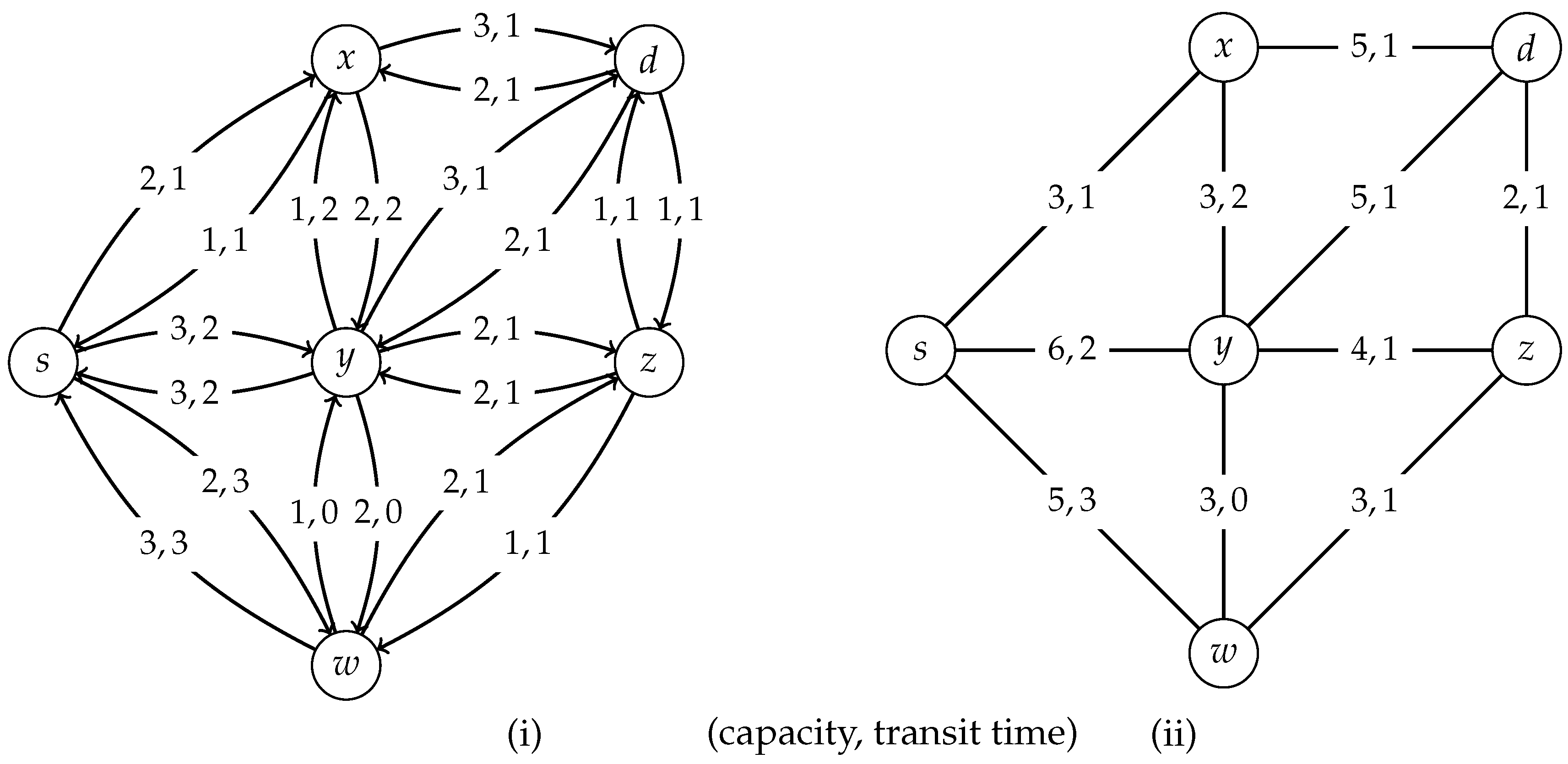
Example 1.
Let us consider a single-source single-sink evacuation network as shown in Figure 1(i), where s is the source node and d is the sink node. The arcs, for example, and , represent the two-way road segments between nodes x and y. Each arc contains capacity and transit time (cost) associated to it. For example, arc has capacity 2 and transit time 3, that means, assuming a time unit of 5 min and a flow unit of 10 cars, a maximum of 20 cars can reach w from s in 15 min. The auxiliary network for reconfiguration is as shown in Figure 1(ii), in which the capacity of each edge is obtained by adding the capacities of and the transit time .
3. Static Partial Contraflow
In this section, we introduce the maximum static partial contraflow problem (MSPCFP) (cf. Problem 1) and the lex-maximum static partial contraflow problem (LMSPCFP) (cf. Problem 2). Thereafter, polynomial time algorithms are presented to solve these problems. These algorithms work as a foundation of solving the dynamic versions of the corresponding problems in the subsequent sections.
3.1. Maximum Static Partial Contraflow
Problem 1.
Given a static network , the maximum static partial contraflow problem (MSPCFP) is to maximize a static S-D flow, saving the unused arc capacity, if the direction of arcs can be reversed partially.
Algorithm 1 is designed for a single-source single-sink static network.
| Algorithm 1: The maximum static partial contraflow algorithm (MSPCFA). |
| Input: A static network Output: A maximum static partial contraflow (MSPCF) on with saved capacities of arcs
|
Step 2 of Algorithm 1 relies on any of the best polynomial time maximum flow algorithms that have a long history but are still under study. Their optimal solutions are guaranteed by the fundamental max-flow min-cut theorem, which states that the maximum flow value equals to the minimum cut capacity. Following the flow augmenting path pseudo-polynomial, that is, time, algorithm of Ford and Fulkerson [13], which ensures a maximum static flow y if and only if the corresponding residual network does not contain an augmenting path, there exist several advancements on its improvements. By scaling the capacities, the running time can be improved to , where represents the integer valued maximum arc capacity. Furthermore, the shortest augmenting path algorithm that uses the unit path length function, the blocking flow algorithm that augments along a maximal set of shortest paths with respect to a blocking flow, and the push-relabel algorithm that functions with nonconservation of flows, except at the source, and sink nodes turn into strongly polynomial time algorithms with complexity, , and , respectively.
The flow decomposition of Step 3 into paths and cycle removal is less costly with running time. In a few special case, like unit capacities, some of these algorithms can be implemented with nearly linear time bounds. Using advanced data structures and dynamic trees, though much theoretical, even more strongly polynomial time algorithms are developed, however, not much implementable in usual practice (see Goldberg and Tarjan [36] for a brief review). For example, with the dynamic-tree data structure, the binary blocking flow algorithm requires time within a factor of the best algorithm for the unit arc capacity problem without parallel arcs.
In Step 4 of Algorithm 1, reversal of traffic flow is allowed only in the necessary amount on the road segment, i.e, partial reversal of the arcs in evacuation network. Unlike in the previous investigations, the remaining capacity of the segment is not reversed, which can be used for other purposes, for example, facility location–allocation and emergency logistic supports.
Based on maximum static contraflow solution with complete contraflow configuration presented in [28], Step 2 of Algorithm 1, the maximum flow algorithm, computes the maximum static flow optimally on auxiliary network and Step 5 comes as a direct consequence of it. This leads to:
Lemma 1.
Algorithm 1 computes the maximum static flow with partial arc reversal on by saving capacities of arc correctly.
Theorem 1.
Algorithm 1 solves the MSPCFP in strongly polynomial time with partial arc reversal capability.
Using a maximum flow algorithm, Rebennack et al. [28] obtained a maximum contraflow solution in auxiliary network. However, their algorithm applies complete arc reversal strategy, such that an arc is reversed if and only or for in the maximum static contraflow solution y. Here, we use partial lane reversal strategy, where the lanes of arcs not required by the contraflow solution are not reversed.
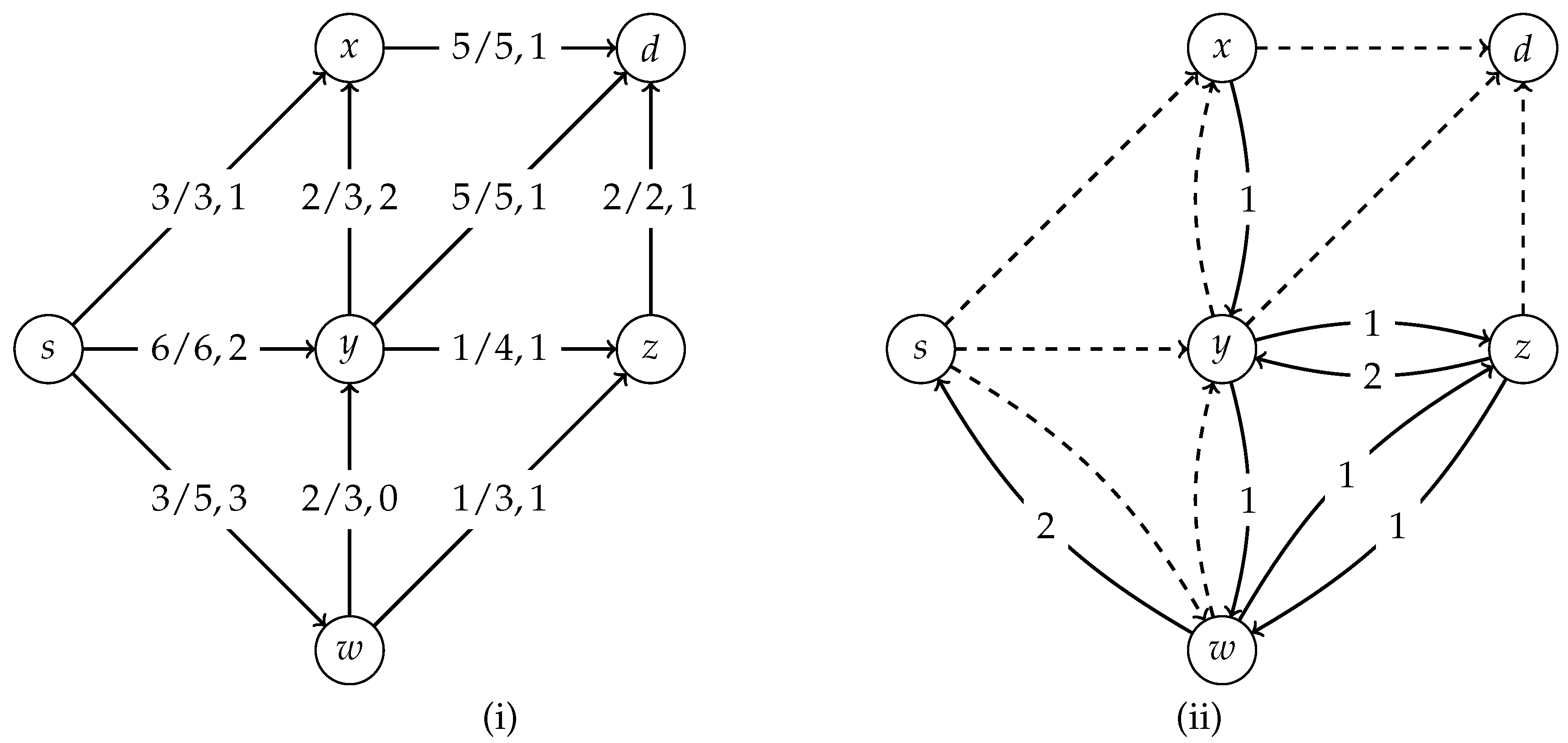
Example 2.
We illustrate Algorithm 1 on the network constructed in Example 1. First, we solve the maximum static flow problem on auxiliary network in Figure 1(ii). As shown in Figure 2(i), paths , , , , and carry 3, 5, 1, 1, and 2 flow units, respectively. Thus, the obtained maximum static flow 12 units on is equivalent to the maximum static contraflow on with arc reversals. According to Algorithm 1, arcs are reversed completely; arcs are partially reversed each up to the capacity 1; each of the arcs has a saved capacity of one unit; and each of has that of two units, as shown in Figure 2(ii).
3.2. Lex-Maximum Static Partial Contraflow
Assume that, in a multiterminal evacuation network, the risk zones and the destination areas are prioritized subject to specific reasons such as risk levels of disastrous areas, disabilities or urgency of the evacuees, and service requirements to them. To meet these necessities, the sets of sources and sinks are categorized as priority sets.
Let and , respectively, be the priority sets of the sources and sinks, where gets higher priority to whenever holds. Considered with a maximal flow, let the greatest number of units that can enter the sink be . Then, a maximal flow that delivers units into each is a lexicographically (lex-) maximal static flow on the sinks. A maximal flow that sends maximum number of units, , out of each is a lexicographically (lex-) maximal flow on the sources.
Problem 2.
Let be a given multiterminal network with ordered sets of sources and sinks. The lex-maximum static partial contraflow problem (LMSPCFP) at sources (sinks) is used to determine a feasible flow that lexicographically maximizes the amounts leaving (entering) the terminals in given priority orders, if the partial reversal of arcs is allowed.
To solve the lex-maximum static partial contraflow problem (LMSPCFP; Problem 2), we design Algorithm 2. An illustration is given in Figure 3.
| Algorithm 2: The lex-maximum static partial contraflow algorithm (LMSPCFA). |
| Input: A multiterminal static network with given orders of sources and sinks priorities Output: A LMSPCF on with saved capacities of arcs
|
The authors of [31] presented a polynomial time algorithm to find contraflow reconfiguration with complete arc reversals. We establish the following result that leaves the unused parts of arcs unturned, solving a lex-maximum partial contraflow problem in polynomial time.
Theorem 2.
The LMSPCFP can be solved using Algorithm 2 in polynomial time with arc reversals partially.
Proof.
For the given priority ordering of multiterminals, the maximum static flow problem is solved iteratively on auxiliary network that gives an optimal solution to the lexicographically (lex-) maximum static flow problem, as in [16]. The obtained solution is equivalent to the lex-maximum static contraflow solution on ,31]. Step 5 of Algorithm 2 saves all unused capacities of arcs in time, leading to the solution of LMSPCFP in polynomial time. ☐
4. Partial Lane Reversals for Time-Invariant Attributes
This section deals with the concepts of dynamic partial contraflow and contra-transshipment problems with constant transit times and capacities on arcs. Some efficient algorithms are presented for their solutions. As the evacuation issues with dynamic environment have been categorized into different problem types, such as maximum flow, quickest flow, lexicographically maximum flow, earliest arrival flow, quickest transshipment, and earliest arrival transshipment, each has to be dealt to separately with contraflow and, thereby, partial contraflow configuration techniques. The maximum dynamic, earliest arrival, lex-maximum dynamic and quickest, dynamic partial contra-transshipment problems are abbreviated by MDPCFP, EAPCFP, LMDPCFP, QPCFP, and DPCTP, respectively.
4.1. Dynamic Contraflow Problems
As there is no algorithm to find temporally repeated flows on general S-D dynamic networks, an exact optimal dynamic contraflow solution for them have not been found in polynomial time yet. In particular, on the networks, like two-terminal s-d; priority-based S-D; and transshipments S-d, s-D, and S-D with different constraints, the optimal static flow can be decomposed into chains (paths) that are temporally repeated over the time horizon, T, returning the temporally repeated dynamic flows in such cases. From the series of literature on analytical contraflow [1,24,28,30,31,32,37], it is established that the optimal dynamic contraflow for the given network is equivalent to the optimal dynamic flow on corresponding reconfigured network . The input network may be a super-source super-sink added extended network if one is considering a multiterminal network, whenever a temporally repeated solution is possible.
Previous contraflow approaches do not apply the remaining arc capacities, which result after contraflow reconfiguration. In this subsection, we redefine a series of partial contraflow problems with time-invariant attributes and present appropriate efficient algorithms to solve the corresponding problems saving the unnecessary arc capacities. Once a dynamic flow is obtained, it should be subtracted from reconfigured capacities of arcs to record the maximum unused arc capacities. These algorithms have great benefit as the remaining unused arc capacities can be used for emergency vehicles and logistics. The following problem is more general, addressing respective partial contraflow problems in a compact form.
Problem 3.
Given a network, , with integer inputs, the dynamic partial contraflow problem (DPCFP) with objective function is to find a dynamic S-D flow optimizing for all time with arc reversals partially.
Problem 3 is stated in an abstract form for a general objective function G without its explicit nature. As per the requirement of the specific problem, we will state it explicitly in the subsequent sections.
Applying Step 2 of Algorithm 3, any technique that computes a temporally repeated flow on reconfigured network is applicable to find an optimal solution to the corresponding contraflow for the original network . During the computation of temporally repeated flows, Step 3 removes the cycle flows, if they exist, so that the simultaneous flows in both directions are not possible. Saving of the unused capacities are recorded in Step 5. Thus, a flow is either along arc e or arc , and its value is not greater than the added arc capacities at all time units. Therefore, the condition of feasibility is satisfied by the algorithm. The optimality depends on the specific objective function.
| Algorithm 3: The dynamic partial contraflow algorithm (DPCFA). |
| Input: A Dynamic network with constant and symmetric transit time, i.e., Output: A dynamic partial contraflow x with the partial arc reversals
|
4.1.1. Maximum Dynamic Contraflow
If the flow has to be maximized for given time period, T, without considering earlier periods, then Problem 3 with the arcs permissible to be reversible only at time zero is the MDPCF problem. The objective (8) is then for subject to constraints (4)–(6).
Polynomial time algorithms to solve the S-D MDCFP has not been investigated yet. However, it can be solved in pseudo-polynomial time by reducing it into extended s-d network of its time-expanded network. The s-d MDCFP is polynomially solvable in discrete time [28] and, in continuous time, [30] reverses an arc completely whenever it is to be reversed.
Theorem 3.
The s-d MDPCFP with can be solved in time in which flow decomposition and minimum cost flow problems are solved in and times, respectively.
Proof.
Theorem 3 is proved in three steps. First, we show that the solution Algorithm 3 yields is feasible. Step 2 uses maximum dynamic flow algorithm of [13]. After the removal of the positive flow in cycles in Step 3, there is a flow either along arc e or but never in both arcs and the flow is not greater than the modified capacities in the auxiliary network on each arc at each time unit. Second, we show the optimality. We use the temporally repeated flow algorithm of [13] after we obtain the feasible flow that gives a maximum dynamic flow solution on reconfigured network , which is equivalent to the maximum dynamic contraflow solution on with the arcs reversed up to the necessary capacity in Step 4. In Step 5, we record the capacities of the arcs not used by the flow after necessary (partial) arc reversals, thereby obtaining a MDPCF solution.
The time complexity of the algorithm is dominated by the time complexity of the maximum dynamic flow algorithm of [13] in Step 2, which is equal to the complexity of a minimum cost flow computation, and that of flow decomposition in Step 3. This completes the proof. ☐
Example 3.
We compute the maximum dynamic flow on auxiliary network (cf. Figure 1(ii)) of evacuation network in Figure 1(i)) having the aforementioned capacities and transit times on each arc with the repetition of path flows computed in Example 2 within given time horizon . Using the algorithm in [13], we get the static flow y corresponding to the temporally repeated dynamic flow, which is the same as that in Figure 2(i). The temporally repeated maximum dynamic flow after partial contraflow configuration is as given in Table 1.
The arc reversals and saved capacities are similar to those in Example 2.
We observe another algorithm for the partial contraflow configuration that is based on the minimum cut problem. The formation of reconfigured network is from weighted undirected network on which a minimum s-d cut can be obtained in time complexity that is independent with maximum flow computations (Karger and Stein [38]). The partial contraflow configuration can be achieved by reversing only the capacities of arcs that are equal to the minimum cut capacities. However, it is difficult to identify the used capacities of other arcs that are not contained on minimum cut set. We can say that maximum flow is equal to the minimum cut but there is not any technique developed to decompose the maximum flow value in different s-d paths in undirected network given a minimum cut solution. If any such technique exists, then solving partial contraflow configuration problem is not harder than finding the distribution of maximum flow value in different arcs and paths of the network.
4.1.2. Earliest Arrival Contraflow
The earliest arrival (also known as the universal maximum) partial contraflow problem (EAPCFP/UMPCFP) on the given dynamic network is to find a dynamic S-D flow that is maximum for all time steps with arc reversal capability partially. In Step 2 of Algorithm 3, the objective function (8) is then for all subject to constraints (4)–(6).
The earliest arrival contraflow problem for s-d series-parallel network is solved in polynomial time , being identical with maximum flow optimal solution in which arcs are reversed only at time zero [29,30]. The two solutions match for this case since each cycle in the residual network has nonnegative length [18]. However, for other general networks, as there does not exist any exact earliest arrival maximum flow solution with standard chain decomposition of [13], the nonstandard chain decomposition of [19] has to be applied in order to decide contraflow reconfiguration which demands arc reversals time to time, [24,31]. This results in a pseudo-polynomial time algorithm, using the successive shortest path algorithms as in [15,16]. A complication for the s-d earliest arrival contraflow solution arises because of the flipping requirements of intermediate arcs with respect to the time.
As the S-D maximum dynamic contraflow problem is -hard, the corresponding S-D earliest arrival contraflow problem is also -hard. However, the authors of [30] obtain an approximate contraflow solution within the factor of the optimal earliest arrival contraflow in polynomial time. For this they run, the fully polynomial time approximation algorithm of [17] and obtain the approximate s-d earliest arrival contraflow in time are used, where .
The authors of [39] extend the results on earliest arrival contraflow problem to the partial lane reversal reconfiguration by saving unused arc capacity. Their algorithms have similar times complexities as without contraflow.
4.1.3. Generalization of Dynamic Contraflow
Given a generalized dynamic lossy network with integer inputs, the generalized earliest arrival partial contraflow problem (GEAPCFP) is to find a generalized maximum flow for all defined in Equation (7), subject to the constraints (4)–(6) with partial arc reversal capability at time zero. If flow is maximized for a given time horizon T only, then the problem is a generalized maximum dynamic partial contraflow problem (GMDPCFP).
As the corresponding contraflow problems on general S-D network are -hard, an additional gain factor on each arc make the partial contraflow problems also -hard on general S-D lossy network, too. However, considering s-d lossy network, the contraflow problems can be solved computing corresponding generalized flows on the auxiliary network in pseudo-polynomial time complexity [40]. Moreover, with the same complexity, we can solve the partial contraflow problems using Algorithm 4 saving all unused arc capacities that can be used for other purposes.
There are different factors that make the flow to be lost during evacuation process. However, we consider a special case in which it is assumed that in each time unit the same percentage of the remaining flow value is lost. Thus, we consider a special case for some constant .
In the reconfigured network, we compute a maximum flow by calculating flow along shortest s-d paths, augmenting this flow, and repeating the process successively until no s-d path exists in the residual network. Then, such a maximum flow constructs an optimal maximum dynamic flow in pseudo-polynomial time with the standard temporally repeated flow technique in time-expanded network.
| Algorithm 4: The generalized dynamic partial contraflow algorithm (GDPCFA). |
| Input: Given a lossy network with integer inputs Output: The resulting flow is GMDPCF and GEAPCF with the arc reversals by saving unused arc capacities
|
Theorem 4.
The generalized maximum dynamic partial contraflow problem (GMDPCFP) can be solved with pseudo-polynomial time complexity.
Proof.
The highest gain path is computed in time, in which transit time is considered as cost function. In auxiliary network the generalized maximum flow using the highest gain path is computed by a standard maximum flow algorithm. For given time horizon T, there are at most T iteration, i.e., a maximum flow is computed at each iterations in , and thus time complexity is [41]. As Steps 2 and 3 are solved in linear time, the complexity of Algorithm 4 is dominated by Step 1. Therefore, the GMDPCFP is solved in time complexity. Moreover, the GMDPCF solution has the earliest arrival property maximizing the flow at each point of time and thus, the GEAPCFP is also solved in the same complexity. ☐
4.1.4. Lexicographically Maximum Dynamic Contraflow
With given priority ordering at terminals of the dynamic network , the LMDPCFP is to find a lexicographically maximum dynamic flow at each priority terminal sets with arc reversal capability partially at any time point.
Fixing the supplies and demands at sources and sinks, the LMDPCFP problem has been solved with polynomial time complexity [24,31]. However, it is also solvable for unknown supplies and demands on terminals with the same complexity, because there is a priority ordering in terminals but not in supplies and demands. In the reconfigured network of Algorithm 3, if we calculate the minimum cost flow in Step 2 at each iteration as in [19], the LMDPCF solution is obtained after (number of terminals) iterations within time horizon T by saving unused arc capacities. However, it uses so-called nonstandard flow decomposition in which backward arcs are allowed. The consequence is Theorem 5.
Theorem 5.
The LMDPCFP with partial reversals of arc capacities can be solved in time, where is the time complexity of minimum cost flow solution.
4.1.5. Quickest Contraflow Problem
Problem 4.
For a given dynamic network with integer inputs and fixed flow value , the quickest partial contraflow problem (QPCFP) is to find a minimum time T to transship the flow value from the sources S to the sinks D with arc reversal capability partially.
The authors of [24,28,30,37] investigate the s-d network quickest contraflow problem and S-D network quickest contra-transshipment problem and present polynomial-time algorithms for their solution. On the S-D network, the quickest contraflow problem is not easier than 3-SAT and PARTITION [28]. However, for an s-d network, they present a strongly polynomial time algorithm with discrete based on the parametric search technique of Megiddo [42] and Burkard et al. [20]). They find an upper bound for the quickest time by computing s-d paths in polynomial time and then use parametric search to find the minimum time before which given flow value is sent to the sink resulting in a strongly polynomial time complexity of . In same time complexity, the quickest contraflow problem is solved in continuous times in [30].
Pyakurel et al. [37] presented the first polynomial algorithm with a time-complexity of a minimum cost flow algorithm to solve the s-d quickest contraflow problem. The s-d quickest contraflow solution has been computed by solving the parametric minimum cost flow problem using the cost scaling algorithm of Lin and Jaillet [43]. It takes time to solve this problem, where is the maximum transit time over all arcs. All the algorithms are presented with complete contraflow configuration.
Replacing the cost scaling algorithm of Lin and Jaillet [43], if we use the cancel and tighten algorithm of Saho and Shigeno [44] in Step 2 of Algorithm 3 that computes the quickest flow by solving the parametric minimum cost flow problem in strongly polynomial time complexity, we get what is stated in Theorem 6 without detailed proof. With this, we not only improve the complexity of algorithm to solve the s-d quickest contraflow problem, but also reverse necessary parts of the road segments saving all unused arc capacities, obtaining the QPCF solution in strongly polynomial time.
Theorem 6.
The quickest contraflow problem on s-d network can be solved in time complexity with partial reversals of arc capacities.
4.2. Dynamic Contra-Transshipment Problems
Problem 5.
Given a network with integer inputs, the dynamic partial contra-transshipment problem (DPCTP) with objective function is to find a feasible dynamic S-D flow for that fulfills the supply-demand shipments with partial arc reversals.
Problem 5 is stated in an abstract form for a general objective function G without its explicit nature. As per the requirement of the specific problem, we will state it explicitly in the subsequent sections.
If the fixed source-sink supply-demand amounts should be shifted within given time horizon T by maximizing G at every time point from the beginning with partial arc reversals, then the problem is earliest arrival partial contra-transshipment (EAPCTP).
The authors of [1,24,32] investigate the earliest arrival contra-transshipment problem and present polynomial time algorithms on multisource or multi-sink networks for specific arc transit times. Moreover, a pseudo-polynomial time algorithm has been presented and its approximation solution is computed for arbitrary transit times on each arc. If the transit time of each arc is zero, then the approximation solution is obtained in polynomial time. For an urban evacuation scenarios including life boats or pick-up bus stations, the concept of zero transit time is very important and applicable [45].
Based on the previous results from the literature, the EAPCTP can be solved in different conditions using Algorithm 5 in which all unused arc capacities are saved in contraflow configuration. However, this problem is not solved on general S-D network yet. For the S-d network with arbitrary arc transit times, a solution of the earliest arrival contra-transshipment problem can be found in polynomial time reversing the arc in the time intervals whenever necessary. Moreover, the algorithm records all unused arc capacities.
By constructing extended network of reconfigured S-d network, we can compute with super-source the -d minimum cost flow circulations according to [21] and can save arc capacity using Step 3 of Algorithm 5 as follows.
First, the S-d network is converted into extended network -d network, making all nodes in S intermediate and the total of the supply is assigned to . Moreover, node is connected from d with a dummy arc having infinite capacity. On -d auxiliary network, we obtain a feasible dynamic flow by computing the minimum cost circulation to the dynamic flow on S-d auxiliary network, where units of flow are being sent from the sources in S to d in time T. In this procedure, to overcome from the violation of individual supplies at the source nodes, an earliest arrival flow pattern , i.e., the maximum flow in which for every , is defined on -d network. If , for all , the process is complete. The pattern is obtained polynomially in the input size plus the number of breakpoints. For given pattern with k breakpoints on the S-d network , an earliest arrival transshipment can be obtained by computing a transshipment dynamic flow in -d network with k additional nodes and arcs. Thus, the obtained earliest arrival transshipment is equivalent to the earliest arrival contra-transshipment on S-d network . Moreover, we can save all the unused arc capacities within the same complexity.
| Algorithm 5: The dynamic partial contra-transshipment algorithm (DPCTPA). |
| Input: A dynamic network with constant and symmetric transit times, i.e., Output: A dynamic contra-transshipment with the partial arc reversals
|
Theorem 7.
On the S-d network, the EAPCTP can be solved in polynomial time in the input plus output size.
If the network is s-D with arbitrary transit times, its solution does not exist, because there is always conflict of which s-D path should be used first to make earliest possible flows. However, if transit times are assumed to be zero, every s-D path has same length yielding optimal earliest arrival contra-transshipment solution in polynomial time. Different networks can be categorized as in [45], wherein the s-D network EAPCTP can be solved polynomially using Algorithm 5 with reversing the partial capacities of arcs.
Theorem 8.
The EAPCTP problem can be solved polynomially on multi-sink networks with transit time zero on each arc, saving the unused arc capacities.
Even with the zero transit times, for the S-D network, an earliest arrival transshipment solution is not possible. Consider a network with two sources, and ; two sinks, and ; and arcs , and . Each source and sink have supply 2 and demand 2, and each arc has unit capacity. If we use all paths at time zero, we can transship three units of flows. But leaving the path - empty, we can transship only two units of flow at time zero violating the maximality at every time point.
Thus, we investigate for an approximate solution for the S-D network earliest arrival partial contra-transshipment problem. For the solution, the reconfigured S-D transshipment network is transformed into time-expanded network. Then, the extended time-expanded network is constructed adding supper source and super sink with enough time bound, T, in which we can apply the algorithm of Gross et al. [23] that computes 2-value approximate earliest arrival transshipment solution. The optimal earliest arrival transshipment solution is bounded by 2 times the earliest arrival transshipment solution, called the 2-value approximate earliest arrival transshipment. It is equivalent to the 2-value approximate earliest arrival contra-transshipment on given network with arbitrary transit time on each arc. As it works on a time-expanded network, its time complexity is pseudo-polynomial. However, if the transit time is reduced to be zero, polynomial time 2-value approximation EAPCT can be obtained using the algorithm in [46] on Step 2 of Algorithm 5, thereby reversing the necessary parts of the segments and saving unused arc capacities in Steps 4 and 5.
Theorem 9.
The 2-value approximated EAPCT on S-D network can be solved efficiently by saving all unused arc capacities of arcs.
5. Lane Reversals with Variable Attributes
We consider problems with variable transit times as a nonlinear function of probable congestion due to the current situation of flow in arcs. The transit times are flow dependent if they depend upon the density, speed and flow rate along the arcs. The inflow-dependent transit time depends on inflow rate at given time point so that, at a time, the flow units enter an arc e with uniform speed which remains uniform throughout this arc.
Contraflow with Inflow Dependent Transit Times
To introduce the inflow-dependent quickest partial contraflow problem (IFDQPCFP), the function in Problem 4 is replaced by inflow-dependent transit time function , which comprises functions , which denote the transit time on arc e if the inflow rate is , for each (see also [47]). In what follows, we model the problem and present a strongly polynomial time algorithm for an approximate solution of IFDQPCFP.
In oder to model the inflow-dependent flow over time problem, assume that at any moment of time the transit time function on an arc is given as a piecewise constant, nondecreasing, left-continuous function of inflow rate, Köhler et al. [2]. Note that this function can be restricted to be only integral values as it can be easily relaxed to allow arbitrary rational values by scaling the time with a proper way. Moreover, any general non-negative, nondecreasing, left-continuous function has been approximated by a step function within arbitrary precision.
Along with the inflow rate, the transit time functions generally depend on the free flow transit time and capacity of the arc. If the capacity of an arc is increased, more flow can be sent along the arc and the units of flow take less time to travel the same arc. In a contraflow configuration, the auxiliary network is constructed by adding the capacities of the opposite arcs. Therefore the same amount of flow may take less time to reach from one end of the arc to the other end in comparison to the one without contraflow configuration. We assume that the free flow transit time in the two opposite arcs and the arc with which they are replaced with in the contraflow configuration are identical. The value of the transit time function on the arc in the auxiliary network is the result of the free flow transit time and the enhanced capacity. We assume that the transit time on an arc e is a function of the inflow rate , the free flow transit time , and the capacity . Our approach is to find the quickest flow in the form of a temporally repeated static flow y, we assume that is given as a function of the static flow rate , , . Let
Then, for some , assuming that the free flow transit times on the opposite arcs e and are equal, we have,
and on the auxiliary network
We present Algorithm 6 to solve the single-source single-sink IFDQPCF Problem 6.
Problem 6.
Given a network with inflow-dependent τ, integer inputs, and fixed flow value , the s-d inflow-dependent quickest partial contraflow problem (IFDQPCFP) is to find a minimum time T to transship the flow value allowing partial arc reversals.
| Algorithm 6: Inflow dependent quickest partial contraflow algorithm (IFDQPCFA). |
| Input: Given a dynamic network Output: An inflow-dependent quickest contraflow allowing partial arc reversals
|
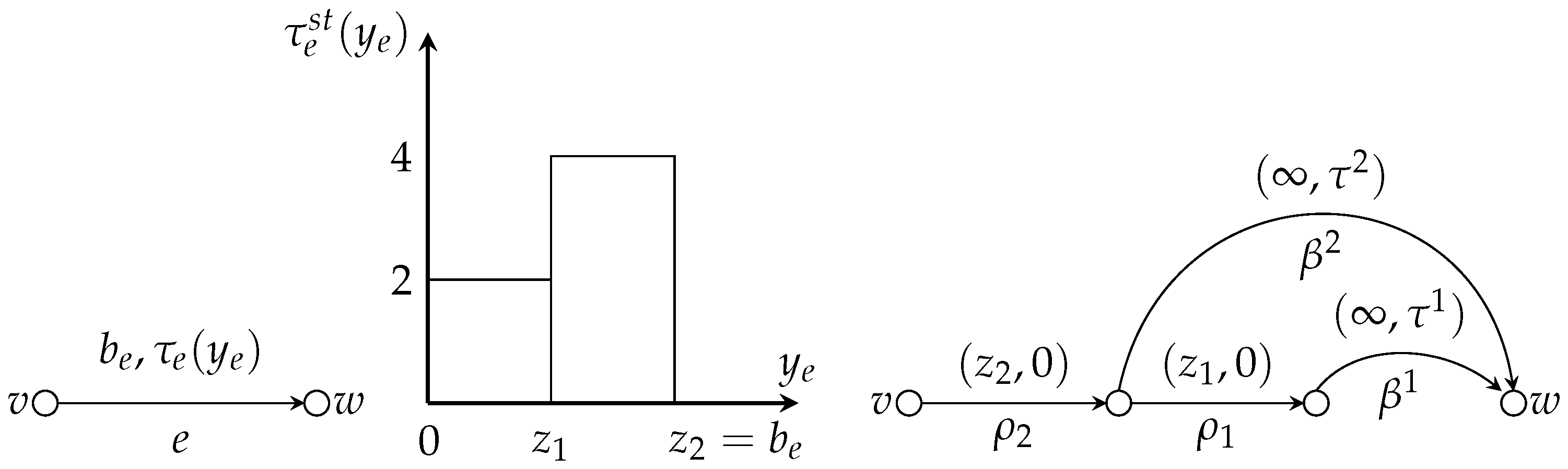
Before we realize the correctness of Algorithm 6, we show that the temporally repeated flow with inflow-dependent transit times can be computed using a bow network in Step 2 as in Köhler et al. [2]. Let be the step function representation of , such that for a particular arc , , where and are non-negative integers. To construct the bow graph, we introduce
- (i)
- regulating arcs with capacity and transit time 0, such that the tail of is the head of for and tail of is v, and
- (ii)
- bow arcs with infinite capacity and transit time such that the tail of is the head of and the head of is w.
Figure 4 shows the bow graph representation of in which .
We denote the bow network corresponding to the network by , where consist of vertices and arcs constructed as a result of bow graph representation of each arc ; and represent the capacity and transit time of each as defined above. With this, every flow over time with inflow-dependent transit times in can be considered as a flow over time with constant transit times in , but not conversely. The problem on bow network is certainly a relaxation of the original with inflow-dependent transit times flow over time problem. Lemma 2 assumes inflow-dependent nondecreasing piecewise constant transit time functions.
Lemma 2.
For given dynamic s-d flow with inflow-dependent transit times sending units in reconfigured network within time , a temporally repeated flow with inflow-dependent transit times can be computed in strongly polynomial time that sends the same amount of s-d flow within at most 2 time.
Proof.
To construct the bow graph of , we modify E by replacing each by two opposite arcs, each with the capacity and transit time , which can be done in times. Then we construct the bow network as mentioned earlier. As this network has constant transit time on arcs, we can use any algorithm to calculate the quickest flow for a network with constant transit time on arcs. The best-known strongly polynomial algorithm so far is the cancel-and-tighten algorithm in [44]. Let be the quickest time to send a flow of value from s to d. Thus, is a lower bound on the optimal time in . The quickest flow computation, e.g., by cancel-and-tighten algorithm, yields a static flow on . Temporal repetition of over the time horizon yields a dynamic flow in , with
The dynamic flow in may not yield a feasible dynamic flow in [2]. We overcome the difficulty by pushing the static flow from fast bow arcs to the slowest positive flow carrying bow arc (say, ) for each . This results into a modified static flow , with val val, which induces a temporally repeated dynamic flow in with time horizon . T can be calculated by using the equation
One can show that
and as val is an increasing function of T, it can be realized that . For any , as uses at most one bow arc , we can find a feasible dynamic flow x in such that . As the temporally repeated dynamic flow induced by satisfies flow conservation, x also satisfies the flow conservation with storage of flow at intermediate nodes on . The time horizon of x is T such that . ☐
Theorem 10.
An approximate solution to the IFDQPCFP can be obtained using the IFDQPCFPA (Algorithm 6) in strongly polynomial time by reversing arc capacities partially.
Proof.
First, the IFDQPCFPA algorithm (cf. Algorithm 6) is feasible, as all of its steps are feasible. On auxiliary network , we can compute the temporally repeated flow with inflow-dependent transit times using the algorithm of Köhler et al. [2] that gives the approximate quickest flow as in Lemma 2 as well as we can save all the unused arc capacities. From the feasibility of our algorithm, we directly conclude that every feasible quickest flow solution on the reconfigured network is equivalent to the quickest flow solution in the original network as in constant transit times [28,30,32]. Thus, the obtained approximate quickest flow on is the approximate quickest partial contraflow for network with inflow-dependent transit times which can be obtained in polynomial time complexity. ☐
6. Case Illustration
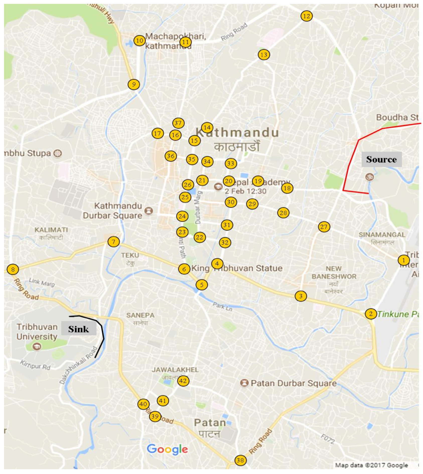
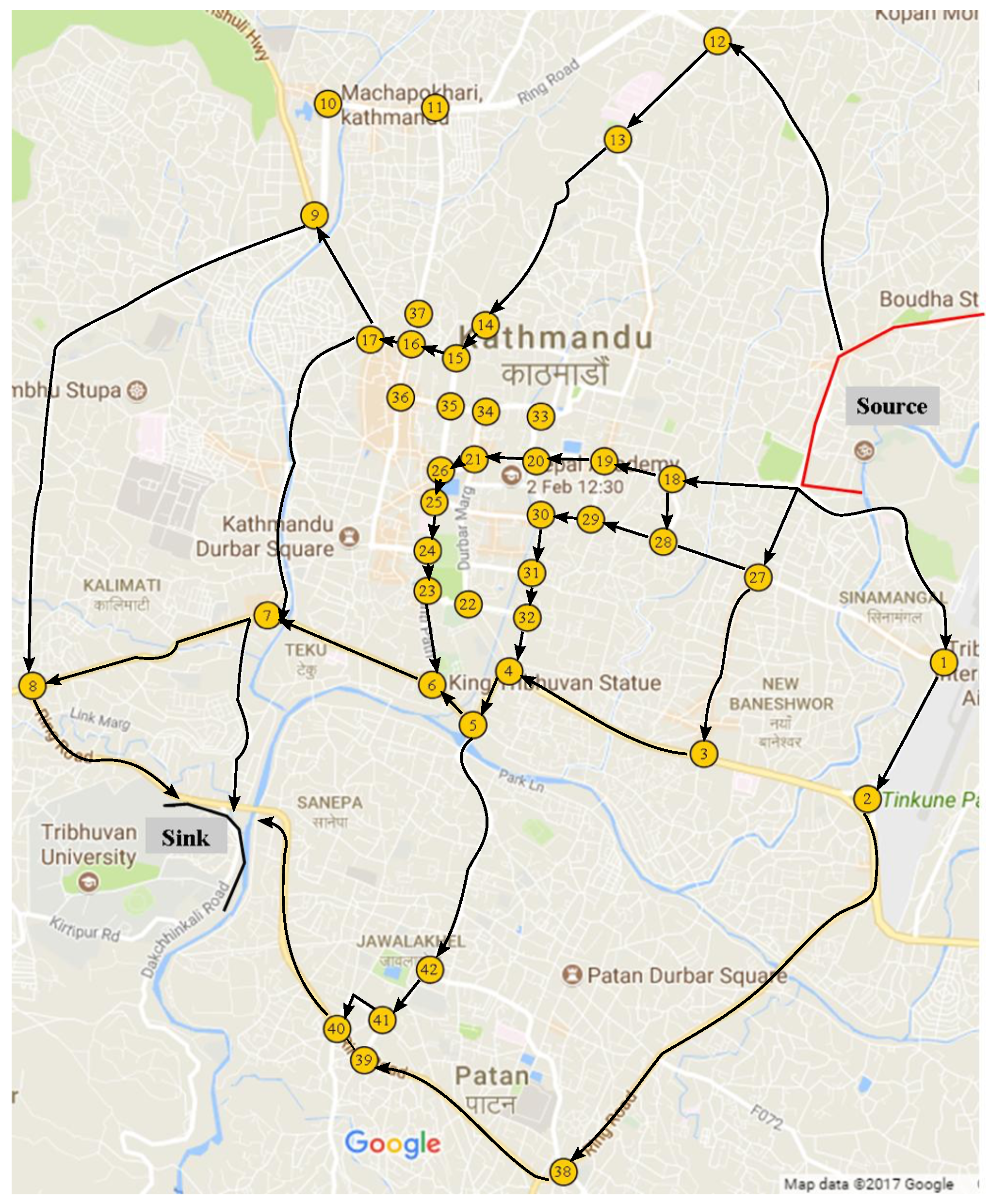
To illustrate some computational results, we consider Kathmandu road network containing major road sections (cf. Figure 5) as an evacuation network N with and . The transit time (which we consider as the free flow transit time) in each road segment is as provided by Google Maps, and the integer capacity is assumed to be between 1 to 4 flow units per second according to the width of the segment. Related data are given in Appendix A (Table A1 and Table A2).
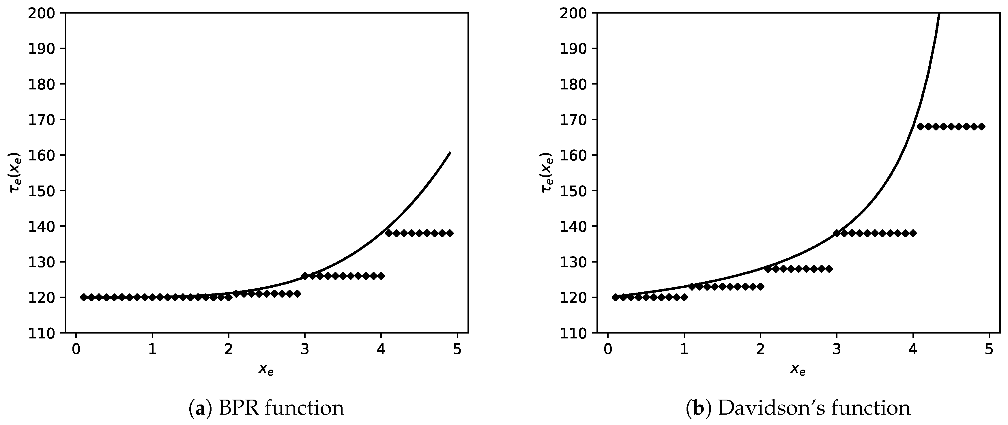
For the purpose of calculating inflow-dependent transit time on each arc e, we consider the following two functions given in [48] and present an analysis corresponding to each of them in parallel.
- BPR function, developed by US Bureau of Public Roads:As an usual practice, we take .
- Davidson’s function:In our computations, we take .
Given the number of flow units to be evacuated, to find the quickest flow allowing (partial) arc reversal, we construct the auxiliary network of the evacuation network. To solve the problem with the transit time depending on the inflow on each arc, we construct the bow graph of the auxiliary network as described in Section 5.
To construct the bow graph, measuring in flow units per second and in seconds, we consider the transit time function as the step function
where represents the least integer greater than or equal to and is the value of rounded to the nearest integer. As an example, the step function representation of a function on an arc with the free flow transit time 120 s and capacity four units of flow per second is given in Figure 6.
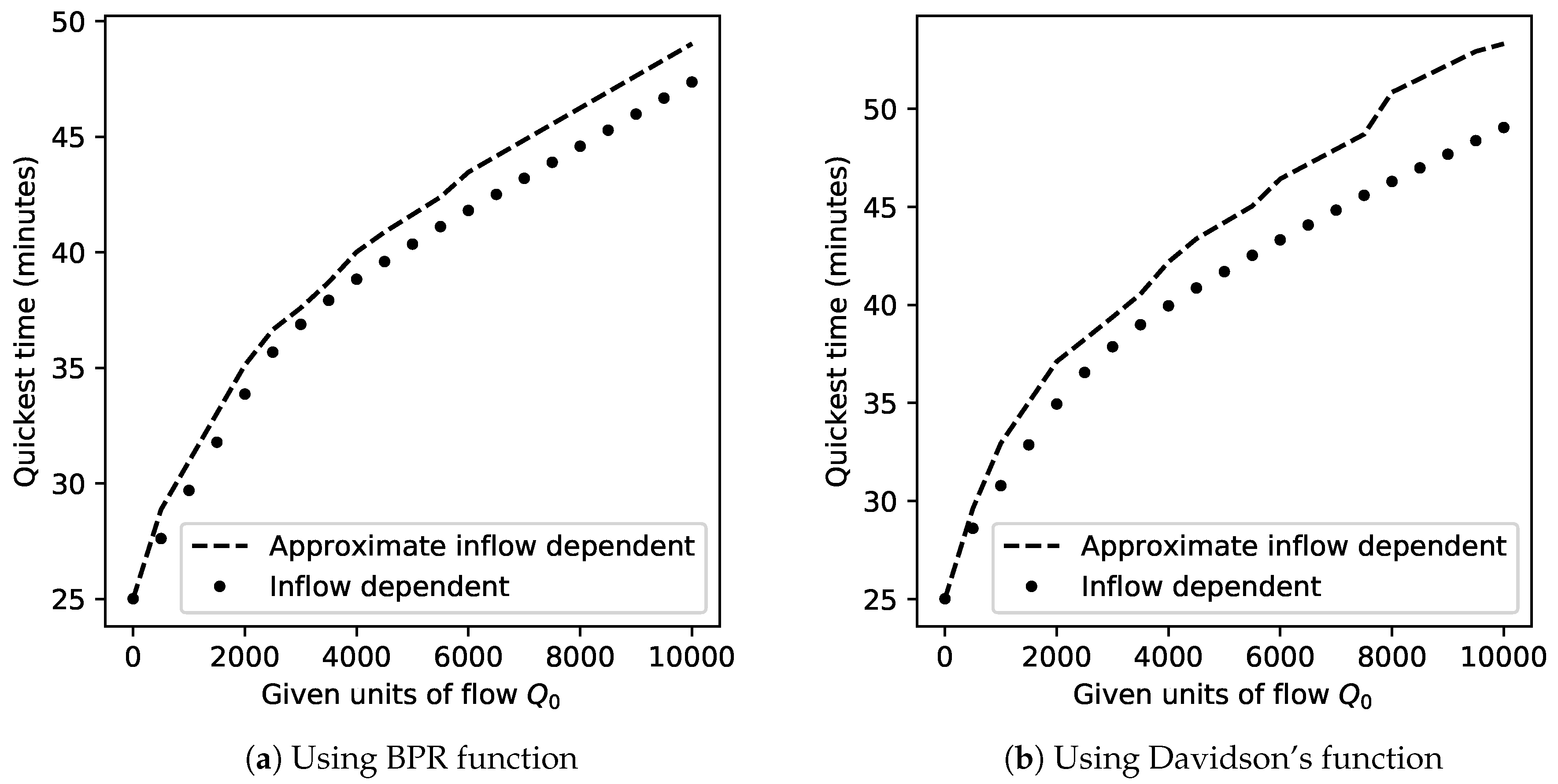
We find the static flow corresponding to the quickest flow in the bow graph, and we push the flow to the slowest arc (see Section 5) to find the approximate dynamic flow corresponding to the quickest flow. To compare the quickest time in the bow graph and its approximate value , we consider between 1 to 10,000 with a gap of 500. The results are shown in Figure 7. We find the maximum value of to be in case of BPR function and in case of Davidson’s function.
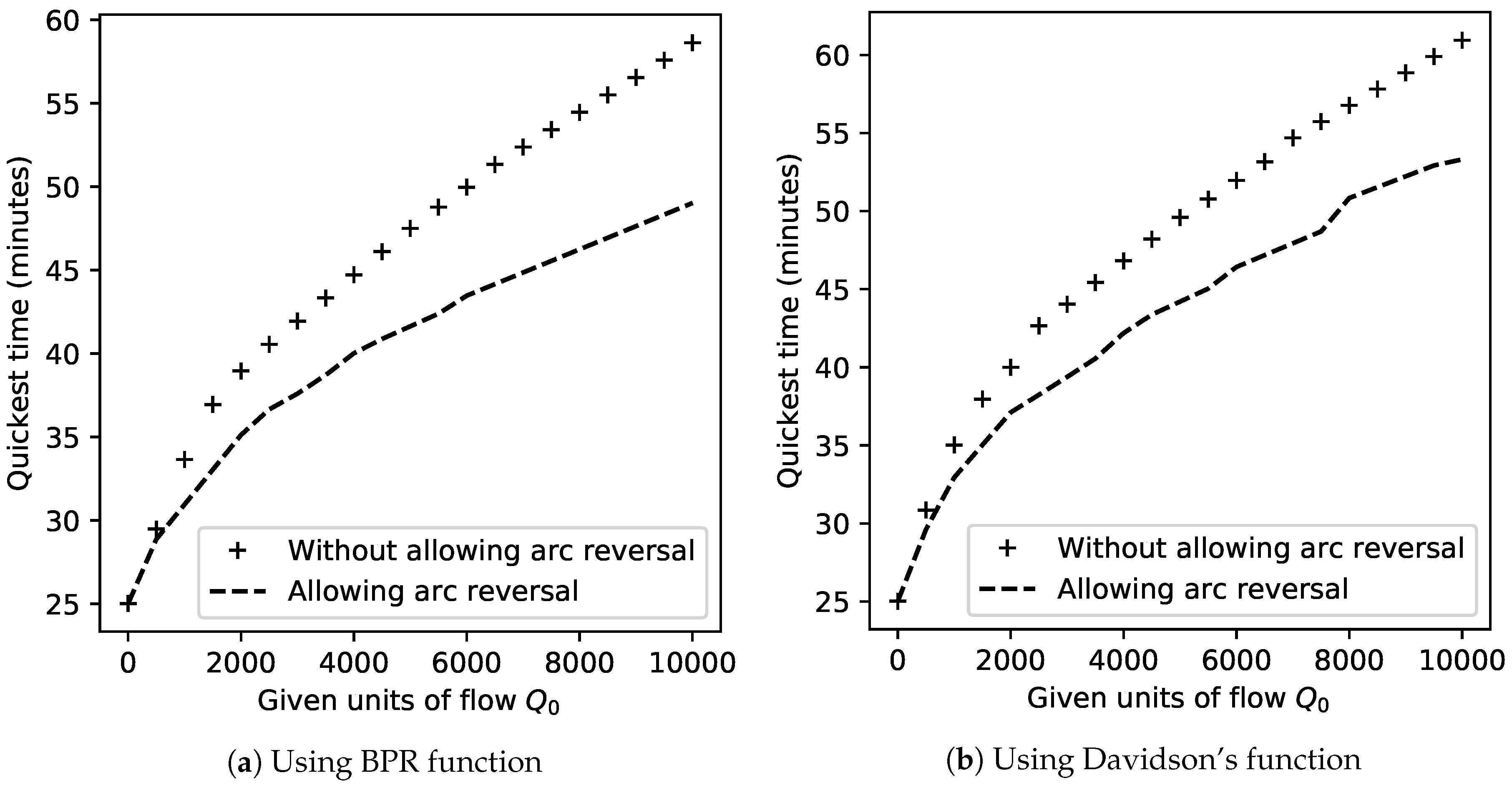
We compare the quickest times before and after allowing partial arc reversal in Figure 8. For as small as 500, the quickest time before allowing (partial) arc reversal using the BPR function is approximately 29.5 min; whereas, after allowing arc reversal, it is 27.6 min (i.e., approximately 93.5% of the time before allowing arc reversal). With the increase in the value of , the gap increases. For as large as 100,000, the value after allowing arc reversal is 141.7 min, 57.6% of the value before allowing arc reversal which is 246.1 min. The quickest times for some values of before and after allowing arc reversal are listed in Table 2.
The number of arcs reversed (partially) for some values of are given in Table 3. The observations show that increasing beyond a sufficient large value does not increase the number of arcs reversed beyond some fixed value (e.g., 29 in this case).
The links used for the quickest flow corresponding to 100,000 allowing partial arc reversal (using BPR function and Davidson’s function) are depicted in Figure 9, with appropriate direction of the flow. The road segments which need to be reversed fully are (1, Source), (12, Source), (18, Source), (27, Source), (2, 1), (13, 12), (14, 13). (15, 14). (5, 4), (7, 6), (Sink, 8), (17, 16), (16, 15), (Sink, 7), (Sink, 40). The segments which are to be reversed partially are listed in Table 4.
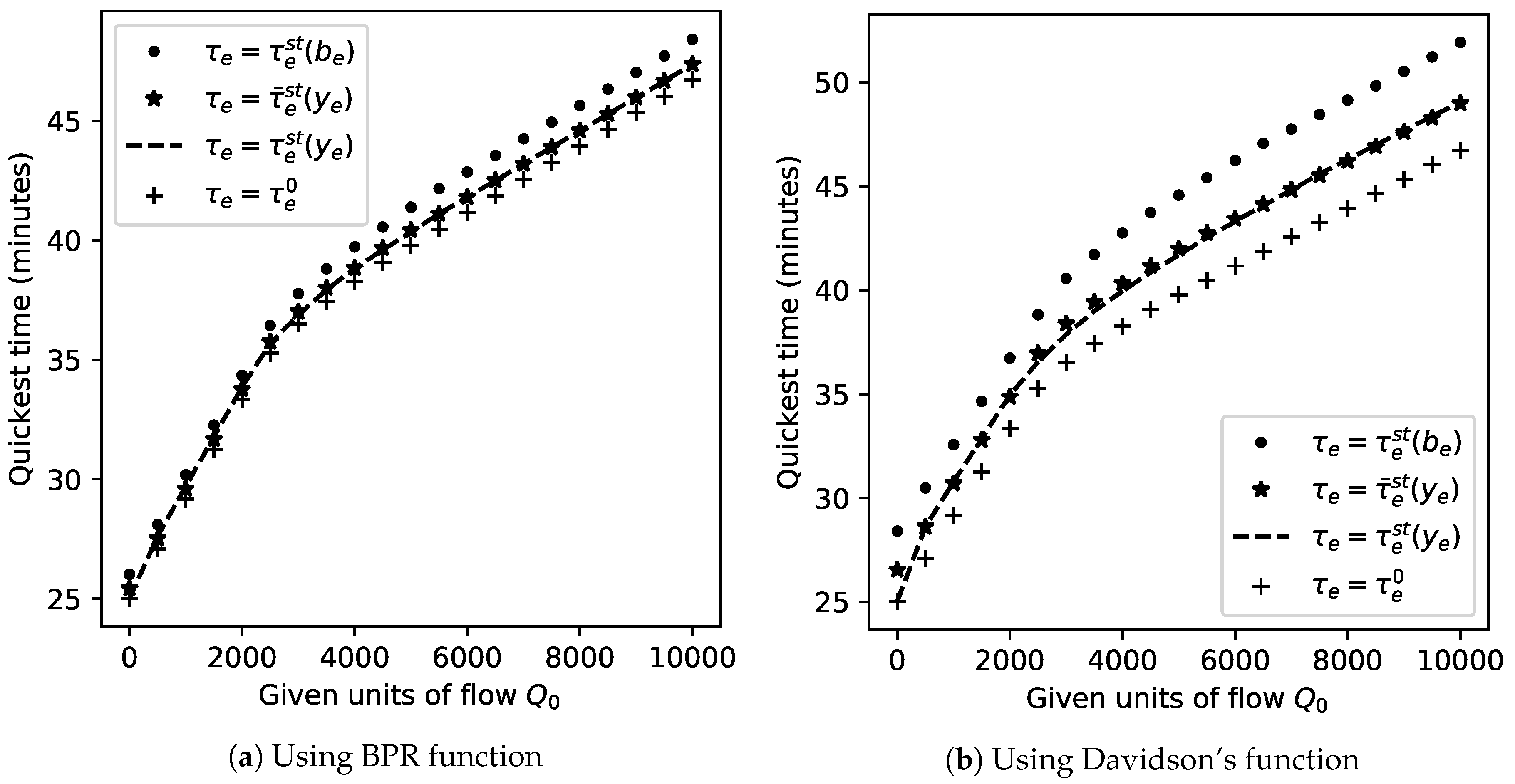
We also compare the quickest times with inflow-dependent transit time on arcs against the quickest times with constant transit time on arcs. For the purpose, we consider three types of constant transit time for each :
- (i)
- , the upper bound on the step function represent of .
- (ii)
- , the average of the step function values.
- (iii)
- the free flow transit time.
It is observed, in the network considered, that the quickest times corresponding to the constant time on each arc as the average of the corresponding step function are very close to the quickest time with inflow-dependent transit time (cf. Figure 10).
7. Conclusions
Highlighting the overall pros and cons of the complete contraflow models and algorithms, a new and more relevant approach—a partial lane reversal strategy—has been introduced in this paper. Using this approach, we can send maximum evacuees in minimum evacuation time recording all unused capacities of the lanes for other crucial emergency and logistic supports for the evacuees with partial reversals of lane capacities. The static partial contraflow problems and the dynamic partial contraflow problems including, the maximum dynamic, the earliest arrival, quickest, lex-maximum dynamic, generalized universally maximum, and partial contra-transshipment problems, have been solved with efficient algorithms. The maximum dynamic and earliest arrival contraflow problems are generalized on lossy networks with partial contraflow reconfiguration. Polynomial time algorithms to solve these problems with constant transit time on each arc have been proposed.
Moreover, the partial contraflow models with variable transit time on each arc have been introduced for the first time. For the inflow-dependent transit times on each arc, an algorithm with strongly polynomial time complexity has been presented that computes an approximate solution to the two terminal quickest contraflow problem with partial lane reversals, which is substantiated by numerical computations considering a case of Kathmandu road network as an evacuation network. The algorithms related to static flow are useful when one is interested to find the maximum rate of flow (evacuees) that can reach the sink(s). Within a specified time, if the maximum number of evacuees have to be evacuated, algorithms related to maximum dynamic flow are useful. The algorithms related to quickest flow are useful to identify the minimum time to evacuate a known number of evacuees.
To the best of our knowledge, the problems investigated in this work are conducted for the first time in the partial contraflow approach. Although these models provide information about the parts of the road segments not used by evacuees, they do not guarantee the existence of such a path between given nodes which may be required for movement of facilities from a node towards sources. As we have investigated only a single-source single-sink model with variable attributes to identify the quickest time, we are interested to extend these contraflow and partial contraflow models and algorithms to solve other network flow over time problems with variable attributes. In addition, we intend to implement the results for supporting logistics in emergencies using the partial contraflow techniques.
Author Contributions
Conceptualization, U.P.; Formal analysis, U.P. and H.N.N.; Investigation, U.P. and H.N.N.; Supervision, S.D. and T.N.D.; Writing–original draft, U.P.; Writing–review and editing, H.N.N.
Funding
This research received no external funding.
Acknowledgments
This research has been carried out during the stay of the first author as a research fellow with George Foster Fellowship for Post-doctoral Research and the stay of the third the author under the AvH Research Group Linkage Program at TU Bergakedemie Freiberg, Germany. The authors acknowledge the support of the Alexander von Humboldt Foundation, and thank the anonymous reviewers for their worthwhile suggestions to improve the quality of this work.
Conflicts of Interest
The authors declare no conflicts of interest.
Abbreviations
The following abbreviations are used in this manuscript:
| BPR | Bureau of Public Roads |
| DPCFA | Dynamic partial contraflow algorithm |
| DPCFP | Dynamic partial contraflow problem |
| DPCTA | Dynamic partial contra-transshipment algorithm |
| DPCTP | Dynamic partial contra-transshipment problem |
| EAPCFA | Earliest arrival partial contraflow algorithm |
| EAPCFP | Earliest arrival partial contraflow problem |
| GDPCFA | Generalized dynamic partial contraflow algorithm |
| GDPCFP | Generalized dynamic partial contraflow problem |
| GEAPCFA | Generalized earliest arrival partial contraflow algorithm |
| GEAPCFP | Generalized earliest arrival partial contraflow problem |
| GMDPCFA | Generalized maximum dynamic partial contraflow algorithm |
| GMDPCFP | Generalized maximum dynamic partial contraflow problem |
| IFDQPCFA | Inflow-dependent quickest partial contraflow algorithm |
| IFDQPCFP | Inflow-dependent quickest partial contraflow problem |
| LMDPCFA | Lexicographic maximum dynamic partial contraflow algorithm |
| LMDPCFP | Lexicographic maximum dynamic partial contraflow problem |
| LMSPCFA | Lexicographic maximum static partial contraflow algorithm |
| LMSPCFP | Lexicographic maximum static partial contraflow problem |
| MDPCFA | Maximum dynamic partial contraflow algorithm |
| MDPCFP | Maximum dynamic partial contraflow problem |
| MSPCFA | Maximum static partial contraflow algorithm |
| MSPCFP | Maximum static partial contraflow problem |
| QPCFA | Quickest partial contraflow algorithm |
| QPCFP | Quickest partial contraflow problem |
| UMPCFA | Universal maximum partial contraflow algorithm |
| UMPCFP | Universal maximum partial contraflow problem |
Appendix A

Table A1.
Network data considered in Section 6.
Table A1.
Network data considered in Section 6.
| e | (per second) | (per second) | (minutes) |
|---|---|---|---|
| (Source, 1) | 2 | 2 | 6 |
| (Source, 12) | 2 | 2 | 10 |
| (Source, 18) | 2 | 2 | 3 |
| (Source, 27) | 2 | 2 | 4 |
| (1, 2) | 2 | 2 | 3 |
| (1, 27) | 2 | 2 | 5 |
| (2, 3) | 3 | 3 | 5 |
| (2, 38) | 3 | 3 | 12 |
| (3, 4) | 3 | 3 | 5 |
| (3, 27) | 2 | 2 | 6 |
| (4, 5) | 3 | 3 | 1 |
| (4, 32) | 2 | 2 | 1 |
| (5, 6 ) | 3 | 3 | 1 |
| (5, 42) | 2 | 2 | 7 |
| (6, 7) | 3 | 3 | 5 |
| (6, 23) | 2 | 2 | 2 |
| (7, 8) | 3 | 3 | 8 |
| (7, 17) | 2 | 2 | 10 |
| (7, Sink) | 2 | 2 | 5 |
| (8, 9) | 2 | 2 | 16 |
| (8, Sink) | 3 | 3 | 7 |
| (9, 10) | 2 | 2 | 3 |
| (9, 17) | 2 | 2 | 3 |
| (10, 11) | 2 | 2 | 5 |
| (11, 12) | 2 | 2 | 17 |
| (11, 37) | 2 | 2 | 7 |
| (12, 13) | 2 | 2 | 4 |
| (13, 14) | 2 | 2 | 6 |
| (13, 33) | 2 | 2 | 9 |
| (14, 15) | 2 | 2 | 1 |
| (14, 33) | 2 | 2 | 3 |
| (15, 16) | 2 | 2 | 1 |
| (15, 35) | 2 | 2 | 1 |
Table A2.
Network data considered in Section 6 (contd…).
Table A2.
Network data considered in Section 6 (contd…).
| e | (per second) | (per second) | (minutes) |
|---|---|---|---|
| (16, 17) | 2 | 2 | 1 |
| (16, 36) | 2 | 2 | 3 |
| (16, 37) | 4 | 0 | 1 |
| (18, 19) | 2 | 2 | 2 |
| (18, 28) | 2 | 2 | 2 |
| (19, 20) | 2 | 2 | 2 |
| (19, 29) | 2 | 2 | 2 |
| (20, 21) | 2 | 2 | 2 |
| (20, 30) | 2 | 2 | 2 |
| (20, 33 ) | 2 | 2 | 1 |
| (21, 26) | 0 | 4 | 1 |
| (21, 34) | 2 | 2 | 1 |
| (22, 23) | 4 | 0 | 1 |
| (22, 32) | 2 | 2 | 1 |
| (23, 24) | 4 | 0 | 1 |
| (24, 25) | 4 | 0 | 2 |
| (25, 26) | 4 | 0 | 1 |
| (26, 35) | 2 | 2 | 2 |
| (27, 28) | 2 | 2 | 3 |
| (28, 29) | 4 | 0 | 2 |
| (29, 30) | 4 | 0 | 1 |
| (30, 31) | 2 | 2 | 2 |
| (31, 32) | 2 | 2 | 2 |
| (33, 34) | 2 | 2 | 2 |
| (34, 35) | 2 | 2 | 1 |
| (35, 36) | 2 | 2 | 2 |
| (38, 39) | 3 | 3 | 7 |
| (38, 42) | 2 | 2 | 8 |
| (39, 40) | 3 | 3 | 1 |
| (39, 41) | 2 | 2 | 1 |
| (40, 41) | 2 | 2 | 2 |
| (40, Sink) | 3 | 3 | 8 |
| (41, 42) | 2 | 2 | 2 |
References
- Pyakurel, U.; Dhamala, T.N.; Dempe, S. Efficient continuous contraflow algorithms for evacuation planning problems. Ann. Oper. Res. 2017, 254, 335–364. [Google Scholar] [CrossRef]
- Köhler, E.; Langkau, K.; Skutella, M. Time expanded graphs for flow depended transit times. In European Symposium on Algorithms; Springer: Berlin/Heidelberg, Germany, 2002; pp. 599–611. [Google Scholar]
- Dhamala, T.N. A survey on models and algorithms for discrete evacuation planning network problems. J. Ind. Manag. Optim. 2015, 11, 265–289. [Google Scholar] [CrossRef]
- Hamacher, H.W.; Tjandra, S.A. Mathematical modeling of evacuation problems: A state of the art. In Pedestrain and Evacuation Dynamics; Schreckenberger, M., Sharma, S.D., Eds.; Springer: Berlin/Heidelberg, Germany, 2002; pp. 227–266. [Google Scholar]
- Cova, T.; Johnson, J.P. A network flow model for lane-based evacuation routing. Transp. Res. Part Policy Pract. 2003, 37, 579–604. [Google Scholar] [CrossRef]
- Altay, N.; Green, W.G., III. OR/MS research in disaster operations management. Eur. J. Oper. Res. 2006, 175, 475–493. [Google Scholar] [CrossRef] [Green Version]
- Pascoal, M.M.; Captivo, M.E.V.; Climaco, J.C.N. A comprehensive survey on the quickest path problem. Ann. Oper. Res. 2006, 147, 5–21. [Google Scholar] [CrossRef] [Green Version]
- Moriarty, K.D.; Ni, D.; Collura, J. Modeling traffic flow under emergency evacuation situations: Current practice and future directions. In Proceedings of the 86th Transportation Research Board Annual Meeting, Washington, DC, USA, 21–25 January 2007. [Google Scholar]
- Chen, L.; Miller-Hooks, E. The building evacuation problem with shared information. Nav. Res. Logist. 2008, 55, 363–376. [Google Scholar] [CrossRef]
- Yusoff, M.; Ariffin, J.; Mohamed, A. Optimization approaches for macroscopic emergency evacuation planning: A survey. In Proceedings of the International Symposium on Information Technology, Kuala Lumpur, Malaysia, 26–28 August 2008; Volume 3, pp. 1–7. [Google Scholar]
- Dhamala, T.N.; Pyakurel, U.; Dempe, S. A critical survey on the network optimization algorithms for evacuation planning problems. Int. J. Oper. Res. 2018, 15, 101–133. [Google Scholar]
- Kotsireas, I.S.; Nagurney, A.; Pardalos, P.M. Dynamics of disasters—Key concepts, models, algorithms, and insights. In Springer Proceedings in Mathematics & Statistics; Springer: Berlin/Heidelberg, Germany, 2015. [Google Scholar]
- Ford, L.R.; Fulkerson, D.R. Flows in Networks; Princeton University Press: Princeton, NJ, USA, 1962. [Google Scholar]
- Gale, D. Transient flows in networks. Mich. Math. J. 1959, 6, 59–63. [Google Scholar] [CrossRef]
- Wilkinson, W.L. An algorithm for universal maximal dynamic flows in a network. Oper. Res. 1971, 19, 1602–1612. [Google Scholar] [CrossRef]
- Minieka, E. Maximal, lexicographic, and dynamic network flows. Oper. Res. 1973, 21, 517–527. [Google Scholar] [CrossRef]
- Hoppe, B. Efficient Dynamic Network Flow Algorithms. Ph.D. Thesis, Cornell University, Ithaca, NY, USA, 1995. [Google Scholar]
- Ruzika, S.; Sperber, S.; Steiner, M. Earliest arrival flows on series-parallel graphs. Networks 2011, 10, 169–173. [Google Scholar] [CrossRef]
- Hoppe, B.; Tardos, E. The quickest transshipment problem. Math. Oper. Res. 2000, 25, 36–62. [Google Scholar] [CrossRef]
- Burkard, R.E.; Dlaska, K.; Klinz, B. The quickest flow problem. ZOR-Methods Model. Oper. Res. 1993, 37, 31–58. [Google Scholar] [CrossRef]
- Baumann, N.; Skutella, M. Earliest arrival flows with multiple sources. Math. Oper. Res. 2009, 34, 499–512. [Google Scholar] [CrossRef]
- Fleischer, L. Universally maximum flow with piecewise-constant capacities. Networks 2001, 38, 115–125. [Google Scholar] [CrossRef]
- Groß, M.; Kappmeier, J.P.W.; Schmidt, D.R.; Schmidt, M. Approximating earliest arrival flows in arbitrary networks. In European Symposium on Algorithms; Springer: Berlin/Heidelberg, Germany, 2012; pp. 551–562. [Google Scholar]
- Pyakurel, U.; Dhamala, T.N. Continuous dynamic contraflow approach for evacuation planning. Ann. Oper. Res. 2017, 253, 573–598. [Google Scholar] [CrossRef]
- Fleischer, L.; Tardos, E. Efficient continuous-time dynamic network flow algorithms. Oper. Res. Lett. 1998, 23, 71–80. [Google Scholar] [CrossRef] [Green Version]
- Quarantelli, E.L. Evacuation Behavior and Problems: Findings and Implications from the Research Literature; Ohio State University Columbus Disaster Research Center: Columbus, OH, USA, 1980. [Google Scholar]
- Kim, S.; Shekhar, S.; Min, M. Contraflow transportation network reconfiguration for evacuation route planning. IEEE Trans. Knowl. Data Eng. 2008, 20, 1115–1129. [Google Scholar]
- Rebennack, S.; Arulselvan, A.; Elefteriadou, L.; Pardalos, P.M. Complexity analysis for maximum flow problems with arc reversals. J. Comb. Optim. 2010, 19, 200–216. [Google Scholar] [CrossRef]
- Dhamala, T.N.; Pyakurel, U. Earliest arrival contraflow problem on series-parallel graphs. Int. J. Oper. Res. 2013, 10, 1–13. [Google Scholar]
- Pyakurel, U.; Dhamala, T.N. Continuous time dynamic contraflow models and algorithms. Adv. Oper. Res. Hindawi 2016, 2016, 368587. [Google Scholar] [CrossRef]
- Pyakurel, U.; Dhamala, T.N. Models and algorithms on contraflow evacuation planning network problems. Int. J. Oper. Res. 2015, 12, 36–46. [Google Scholar] [CrossRef]
- Pyakurel, U.; Dhamala, T.N. Evacuation planning by earliest arrival contraflow. J. Ind. Manag. Optim. 2017, 13, 489–503. [Google Scholar] [CrossRef] [Green Version]
- Pyakurel, U.; Nath, H.N.; Dhamala, T.N. Partial contraflow with path reversals for evacuation planning. Ann. Oper. Res. 2018. [Google Scholar] [CrossRef]
- Smith, J.M.G.; Cruz, F.R.B. M/G/c/c state dependent travel time models and properties. Phys. Stat. Mechan. Its Appl. 2014, 395, 560–579. [Google Scholar] [CrossRef]
- Ahuja, R.K.; Magnanti, T.L.; Orlin, J.B. Ntwork Flows: Theory, Algorithms, and Applications; Prentice Hall: Englewood Cliffs, NJ, USA, 1993. [Google Scholar]
- Goldberg, A.V.; Tarjan, R.E. Efficient maximum flow algorithms. Commun. ACM 2014, 57, 82–89. [Google Scholar] [CrossRef]
- Pyakurel, U.; Nath, H.N.; Dhamala, T.N. Efficient contraflow algorithms for quickest evacuation planning. Sci. China Math. 2018, 61, 2079–2100. [Google Scholar] [CrossRef]
- Karger, D.R.; Stein, C. A new approach to the minimum cut problem. J. ACM 1996, 43, 601–640. [Google Scholar] [CrossRef]
- Pyakurel, U.; Dempe, S. Earliest arrival flow with partial lane reversals for evacuation planning. Int. J. Oper. Res. Nepal 2019, 8, 27–37. [Google Scholar]
- Pyakurel, U.; Hamacher, H.W.; Dhamala, T.N. Generalized maximum dynamic contraflow on lossy network. Int. J. Oper. Res. Nepal 2014, 3, 27–44. [Google Scholar]
- Groß, M.; Skutella, M. Generalized maximum flows over time. In Approximation and Online Algorithms; Solis-Oba, R., Persiano, G., Eds.; Springer: Berlin/Heidelberg, Germany, 2012. [Google Scholar]
- Megiddo, N. Combinatorial optimization with rational objective functions. Math. Oper. Res. 1979, 4, 414–424. [Google Scholar] [CrossRef]
- Lin, M.; Jaillet, P. On the quickest flow problem in dynamic networks—A parametric min-cost flow approach. In Proceedings of the Twenty-Sixth Annual ACM-SIAM Symposium on Discrete Algorithms; Society for Industrial and Applied Mathematics: San Diego, CA, USA, 2015; pp. 1343–1356. [Google Scholar]
- Saho, M.; Shigeno, M. Cancel-and-tighten algorithm for quickest flow problems. Networks 2017, 69, 179–188. [Google Scholar] [CrossRef]
- Schmidt, M.; Skutella, M. Earliest arrival flows in networks with multiple sinks. Electron. Notes Discret. Math. 2010, 36, 607–614. [Google Scholar] [CrossRef]
- Kappmeier, J.P.W.; Matuschke, J.; Peis, B. Abstract flows over time: A first step towards solving dynamic packing problems. Theor. Comput. Sci. 2014, 544, 74–83. [Google Scholar] [CrossRef]
- Pyakurel, U.; Dempe, S.; Dhamala, T.N. Network reconfiguration with variable transit times for evacuation planning. In Proceedings of the APORS 2018, Kathmandu, Nepal, 6–9 August 2018; pp. 25–28. [Google Scholar]
- Sheffi, Y. Urban Transportation Networks: Equilibrium Analysis with Mathematical Programming Techniques; Prentice-Hall, Inc.: Englewood Cliffs, NJ, USA, 1984. [Google Scholar]
Figure 1.
(i) Evacuation network . (ii) Auxiliary network of .

Figure 2.
(i) Solution in Figure 1(ii) with (flow/capacity, transit time). (ii) Saved capacities to part (i).
Figure 2.
(i) Solution in Figure 1(ii) with (flow/capacity, transit time). (ii) Saved capacities to part (i).

Figure 3.
On the capacitated static network (i) with 2-sources and 3-sinks having priority ordering of sinks , , and , the lex-maximum static partial contraflow is obtained as in . Flow entering sinks , , and are maximized through paths , , , and , and , respectively, by saving arc unit capacity of arcs and .

Figure 4.
Expansion of a single arc in the bow network with transit times 2 and 4, for at most and flow units, respectively.
Figure 4.
Expansion of a single arc in the bow network with transit times 2 and 4, for at most and flow units, respectively.

Figure 5.
Kathmandu road network.

Figure 6.
Flow-dependent transit time functions and corresponding step functions with = 120 s and be = 4 per second.
Figure 6.
Flow-dependent transit time functions and corresponding step functions with = 120 s and be = 4 per second.

Figure 7.
Quickest time in bow graph and its approximation by pushing the flow to the slowest arc.

Figure 8.
Quickest times before and after allowing partial arc reversal.

Figure 9.
Direction of the approximate quickest flow allowing partial arc reversal, 100,000.

Figure 10.
Comparison of quickest times (inflow-dependent transit time vs. constant transit time on arcs).
Figure 10.
Comparison of quickest times (inflow-dependent transit time vs. constant transit time on arcs).

Table 1.
Maximum dynamic flow computation after partial contraflow configuration (cf. Figure 1).
Table 1.
Maximum dynamic flow computation after partial contraflow configuration (cf. Figure 1).
| Path P | Repeated for | Dynamic Flow Value | |
|---|---|---|---|
| 3 | 2, 3, 4, 5, 6 | 15 | |
| 5 | 3, 4, 5, 6 | 20 | |
| 1 | 4, 5, 6 | 3 | |
| 1 | 5, 6 | 2 | |
| 2 | 6 | 2 | |
| Total | 42 |
Table 2.
Comparison of the quickest time before and after allowing arc reversal.
| BPR Function | Davidson’s Function | |||
|---|---|---|---|---|
| Quickest Time | Quickest Time | |||
| before Contraflow | after Contraflow | before Contraflow | after Contraflow | |
| 500 | 29.5 | 27.6 | 30.8 | 28.6 |
| 1000 | 33.6 | 29.7 | 35 | 30.8 |
| 10,000 | 58.6 | 47.4 | 60.9 | 49 |
| 20,000 | 79.5 | 58.4 | 81.8 | 60.5 |
| 50,000 | 142 | 89.6 | 144.3 | 91.7 |
| 100,000 | 246.1 | 141.7 | 248.4 | 143.8 |
Table 3.
Number of arcs reversed.
| Number of Arcs Reversed | ||
|---|---|---|
| BPR Function | Davidson’s Function | |
| 500 | 8 | 5 |
| 1000 | 8 | 10 |
| 10,000 | 20 | 21 |
| 20,000 | 29 | 29 |
| 50,000 | 29 | 29 |
| 100,000 | 29 | 29 |
Table 4.
Partially reversed segments.
| Segment | Reversed Capacity | Capacity |
|---|---|---|
| (3, 27) | 1 | 2 |
| (38, 2) | 1 | 3 |
| (39, 38) | 1 | 3 |
| (40, 39) | 1 | 3 |
| (6, 5) | 1 | 3 |
| (4, 32) | 1 | 2 |
| (32, 31) | 1 | 2 |
| (8, 7) | 1 | 3 |
| (23, 24) | 2 | 4 |
| (24, 25) | 2 | 4 |
| (26, 21) | 2 | 4 |
| (25, 26) | 2 | 4 |
| (31, 30) | 1 | 2 |
| (19, 18) a | 1 | 2 |
| (7, 17) b | 1 | 2 |
a for Davidson’s function only. b for BPR function only.
© 2019 by the authors. Licensee MDPI, Basel, Switzerland. This article is an open access article distributed under the terms and conditions of the Creative Commons Attribution (CC BY) license (http://creativecommons.org/licenses/by/4.0/).
Share and Cite
MDPI and ACS Style
Pyakurel, U.; Nath, H.N.; Dempe, S.; Dhamala, T.N. Efficient Dynamic Flow Algorithms for Evacuation Planning Problems with Partial Lane Reversal. Mathematics 2019, 7, 993. https://doi.org/10.3390/math7100993
AMA Style
Pyakurel U, Nath HN, Dempe S, Dhamala TN. Efficient Dynamic Flow Algorithms for Evacuation Planning Problems with Partial Lane Reversal. Mathematics. 2019; 7(10):993. https://doi.org/10.3390/math7100993
Chicago/Turabian StylePyakurel, Urmila, Hari Nandan Nath, Stephan Dempe, and Tanka Nath Dhamala. 2019. "Efficient Dynamic Flow Algorithms for Evacuation Planning Problems with Partial Lane Reversal" Mathematics 7, no. 10: 993. https://doi.org/10.3390/math7100993
Note that from the first issue of 2016, this journal uses article numbers instead of page numbers. See further details here.