A Generalized Framework for Analyzing Taxonomic, Phylogenetic, and Functional Community Structure Based on Presence–Absence Data


1
Department of Plant Systematics, Ecology and Theoretical Biology, Institute of Biology, Eötvös University, H-1117 Budapest, Hungary
2
MTA-ELTE-MTM Ecology Research Group, Eötvös University, H-1117 Budapest, Hungary
3
Centre d'Ecologie et des Sciences de la Conservation (CESCO), Muséum national d’Histoire naturelle, CNRS, Sorbonne Université, 75005 Paris, France
4
Department of Environmental Biology, University of Rome ‘La Sapienza’, 00185 Rome, Italy
*
Author to whom correspondence should be addressed.
Mathematics 2018, 6(11), 250; https://doi.org/10.3390/math6110250
Submission received: 17 October 2018
/
Revised: 5 November 2018
/
Accepted: 6 November 2018
/
Published: 12 November 2018
(This article belongs to the Special Issue New Paradigms and Trends in Quantitative Ecology)
Abstract
:Community structure as summarized by presence–absence data is often evaluated via diversity measures by incorporating taxonomic, phylogenetic and functional information on the constituting species. Most commonly, various dissimilarity coefficients are used to express these aspects simultaneously such that the results are not comparable due to the lack of common conceptual basis behind index definitions. A new framework is needed which allows such comparisons, thus facilitating evaluation of the importance of the three sources of extra information in relation to conventional species-based representations. We define taxonomic, phylogenetic and functional beta diversity of species assemblages based on the generalized Jaccard dissimilarity index. This coefficient does not give equal weight to species, because traditional site dissimilarities are lowered by taking into account the taxonomic, phylogenetic or functional similarity of differential species in one site to the species in the other. These, together with the traditional, taxon- (species-) based beta diversity are decomposed into two additive fractions, one due to taxonomic, phylogenetic or functional excess and the other to replacement. In addition to numerical results, taxonomic, phylogenetic and functional community structure is visualized by 2D simplex or ternary plots. Redundancy with respect to taxon-based structure is expressed in terms of centroid distances between point clouds in these diagrams. The approach is illustrated by examples coming from vegetation surveys representing different ecological conditions. We found that beta diversity decreases in the following order: taxon-based, taxonomic (Linnaean), phylogenetic and functional. Therefore, we put forward the beta-redundancy hypothesis suggesting that this ordering may be most often the case in ecological communities, and discuss potential reasons and possible exceptions to this supposed rule. Whereas the pattern of change in diversity may be indicative of fundamental features of the particular community being studied, the effect of the choice of functional traits—a more or less subjective element of the framework—remains to be investigated.
1. Introduction
Presence–absence (p–a) indices of dissimilarity between pairs of objects (usually sites or sample plots) have long been used for various purposes in ecology. Most commonly, these coefficients are calculated for all possible pairs to form a dissimilarity matrix, the starting construct for clustering to obtain a classification, and for metric or nonmetric multidimensional scaling to derive an ordination [1,2]. As alternatives to classical measures, dissimilarity values and their averages for all pairs of sites in an ecological sample may also be considered as expressions of beta diversity (e.g., Magurran [3], but see Baselga [4]). Coefficients used for the latter purpose can be partitioned additively into fractions that reflect the influence and relative importance of various ecological processes driving this phenomenon [5,6,7,8].
The p–a dissimilarity between two sites X and Y depends in most cases on the number of species in which they differ, while in some rare instances on the total number of species in the study area as well. The coefficients are usually standardized into the interval [0, 1], the two extreme values reflecting complete similarity and dissimilarity, respectively. In the classical forms of these functions, it is implicitly assumed that all taxa contribute equally to the calculation of pairwise dissimilarity. These properties are best shown by one of the oldest dissimilarity functions, the Jaccard [9] index, in which the number of differential species is divided by the total number of species of the two sites:
and the Sørensen (1948) index, scaled differently as
with a being the number of shared species, and b and c the number of species unique to sites X and Y, respectively (henceforth called differential species).
JAC = (b + c)/(a + b + c)
SOR = (b + c)/(2a + b + c)
While the operation of (either type of) standardization has been widely accepted, the meaningfulness of giving equal weight to taxa has been questioned, especially in functional ecology (e.g., [10,11]). Two species in which sites X and Y differ may serve the same ecological function in the assemblages, whereas other two differential species may play quite different role in the two sites being compared. If there are many differential species, then it can happen that all species unique to either site are functionally very close to some species present in the other site. Contrariwise, differential species may be fairly unique in their functionality as well, falling quite far from all the species of the other site in this respect. Obviously, such ecologically different situations are not reflected by the classical p–a coefficients: high dissimilarity based on taxon (usually species) lists does not necessarily imply high dissimilarity in ecological functionality of the assemblages. If interest lies in a study of functionality indirectly on the basis of species lists, then existing measures of dissimilarity need to be modified.
In addition to similarity in functional features, two other types of relationship between species deserve attention here. The first is taxonomic relatedness, i.e., the question whether differential species in one site have close (e.g., congeneric or confamiliar) relatives in the other. The second one is free from the inevitable arbitrariness involved in assigning ranks to taxonomic groups, namely phylogenetic distance as measured between two species along a phylogram or a chronogram. Classical p–a dissimilarity measures do not cope with these relationships, whereas it may be desirable to consider taxonomic or phylogenetic distinctness of differential species in calculating dissimilarity of sites. For example, these modified dissimilarities may be used as a proxy for functional dissimilarity in lieu of detailed information on the functional features of species. This latter approach, however, is not entirely without problems [12,13]. Note also that we make clear distinction between “taxon-based” and “taxonomic” in agreement with Cardoso et al. [14]—the first uses a partition of organisms into taxa (mostly species), the second relies on a hierarchical classification reflecting relationships between species—a distinction not always recognized. (For example, in Corbelli et al. [15] and Weinstein et al. [16] “taxonomic” is in fact “taxon-based” in our terminology.)
In this paper, we first overview existing proposals that allow adjustment of species weighting according to functional, taxonomic or phylogenetic relatedness. We show, further, that these generalized dissimilarities may be partitioned into additive fractions that have similar interpretation as those of species-based dissimilarities, and extend the functional approach suggested by Ricotta et al. [17] to taxonomic and phylogenetic data. Following the framework originally suggested by Podani and Schmera [6], all pairwise fractions in a given set of plots (sites etc.) are then considered for illustrating community structure graphically, in a ternary plot. Simple artificial examples and three sets of actual vegetation data will be used to show how the original, species-based method modifies when the taxonomic, phylogenetic and functional distinctness of species is also incorporated into the analysis. Finally, we put forward some hypotheses regarding the mutual relationship of results generated by these methods.
2. Preliminaries
One of the first coefficients of dissimilarity which break with the tradition of giving equal weight to species is due to Izsak and Price [18] who suggested to measure pairwise beta diversity by considering the Linnaean taxonomic separation between differential species. This is in fact a modified Sørensen index written here as
In this, wiY is the minimum rank difference between species i in site X and all species occurring in site Y. It has a value of 0 for shared species, a value of 1 if species i has a congeneric species in site Y, a value of 2 if the taxonomically closest relative of species i in site Y is from the same family, and so on. L is the number of ranks; if species, genus, family, order, class and phylum are used, then L = 6. As a result, the contribution of a differential species in site X to the dissimilarity decreases from 1/(2a + b + c) to 1/[(L – 1) (2a + b + c)] if it has a congeneric relative in site Y. = SOR only in the extreme situation when all differential species are separated at the maximum rank. In general, ≤SOR, that is, taxonomic dissimilarity cannot be higher than species-based dissimilarity.
Minimum taxonomic—or rank—separation between species i and j can be conceived as their pairwise dissimilarity, dij. In order to avoid terminological confusion, however, this coefficient will be called distinctness, while the term dissimilarity will be reserved for site comparisons. Distinctness values take the value of 0 if for species identity and dij = 1 if species i separates from species j at the maximum rank in the Linnaean hierarchy used, with the unit range evenly subdivided according to the number of intermediate ranks. Thus, the weight given to a species i ∈ X in Equation (3) can be written as
and similarly, the weight given to species j ∈ Y can be written as
As Ricotta et al. [17] suggested, this offers the possibility that the dissimilarity between two sites can be calculated using any meaningful form of distinctness. In particular, dij may be based on the functional traits of species or can be derived from phylogenetic information, thus allowing calculation of functional or phylogenetic distinctness, respectively. Ricotta et al. [17] also pointed out that many classical p–a coefficients can be modified to accommodate this change by defining
and replacing b and c with B and C. For example, the so-called generalized Jaccard and Sørensen indices take the following form:
and
JAC’ = (B + C)/(a + b + c)
SOR’ = (B + C)/(2a + b + c)
Since dij ≤ 1, it follows that B ≤ b and C ≤ c, and therefore the generalized versions cannot provide larger values than the classical taxon-based dissimilarity measures. Unfortunately, this aspect does not emerge from Figure 4a of Izsak and Price [18], because they compared their taxonomic Sørensen index with the taxon-based Jaccard index, instead of the corresponding taxon-based Sørensen index. In sum, the major difference between taxon-based p–a coefficients and their generalized versions is that in the first every differential species contributes to the numerator by 1, but this value is lowered to some min{dij} in the generalized versions.
Generalized p–a coefficients may be useful in the same three fields of application as the classical versions, as demonstrated by Ricotta et al. [17] for simulated functional data. Multivariate analysis of sites based on a matrix of JAC’ values calculated using the functional distinctness among species provides a functional ordination of sites. It was shown that due to decreased input dissimilarities this ordination is less prone to the arch effect than the traditional, taxon based ordination. For expressing beta diversity changes along a simulated gradient, classical JAC does not necessarily show the same trend as functional JAC’. This is also true for two additive fractions of functional pairwise beta diversity, to be discussed below in considerable detail.
3. The SDR Simplex and Its Generalization
The starting point is that the p–a dissimilarity between sites may be partitioned into additive fractions. Here we adopt the procedure in which dissimilarity is partly due to richness difference (resulting from species loss or gain), and partly to species replacement (also called turnover, although this term is controversial, Podani and Schmera [6], Carvalho et al. [19]). More formally, Jaccard dissimilarity is decomposed according to
with the latter two terms reflecting relative richness difference (D) and relative species replacement (R), respectively. Together with the complement of dissimilarity, i.e., Jaccard similarity (S), these three fractions always sum to 1:
Therefore, the three quantities determine the position of the given pair of sites in a ternary plot, called the SDR simplex [6]. Examining this position offers evaluation of the relative importance of different assembly processes in determining community structure for the given pair of sites. For instance, if S = D = R = 0.33, then the corresponding point will be in the center of the plot, a position interpreted as a completely balanced effect of three processes. If S = 1, then the point will coincide with the S vertex of the triangle, reflecting complete similarity and no replacement and species loss. A situation with S = 0 will always be manifested as a point falling right onto the D–R edge of the equilateral triangle, its exact position being determined by the relative amount of D and R, i.e., the relative importance of species losses and gains, and species replacement. See Podani and Schmera [6] for many artificial and actual examples illustrating different cases of within-community structure. This two-dimensional plot may be reduced to three 1D simplexes by combining any two fractions and contrasting this with the third one. Obviously, the first such possibility is the Jaccard dissimilarity or beta diversity itself (D + R), as given in Equation (9)—which represents a contrast to similarity (S). Relative richness agreement is obtained as S + R. It is complementary to relative richness difference. Relative nestedness is quantified as D + S, with the condition S > 0, and is antagonistic to relative species replacement. Column 1 in Table 1 is a summary of these relationships.
To define taxonomic, functional and phylogenetic SDR-simplexes, the S, D, and R coefficients are generalized as follows:
with B and C defined by Equation (6) and A = a + b − B + c − C [17].
3.1. Fractions of the Generalized Simplex
The entire simplex approach can be generalized to incorporate the taxonomic, phylogenetic or functional distinctness of species if we use JAC’ and its fractions as given in Equations (7), (11)–(13). A fundamental requirement is that distinctness be measured in the range [0,1] irrespective of the data type. Taxonomic separation of species may be readily expressed by Equations (4) and (5). Phylogenetic distinctness values may be derived from a cladogram in which edges are unweighted or, preferably, weighted by the amount of evolutionary change (phylograms) or time (chronograms)—with normalization to unit range according to the maximum. For functional variables, especially if mixed scale types occur, the use of the Gower formula (as suggested by Podani [20], Podani and Schmera [21] and further extended by Pavoine et al. [22]) is recommended. Although the resulting values lie within the range [0,1], the actual maximum rarely reaches the theoretical one, therefore normalization of Gower dissimilarities to unit range is recommended using the maximum observed dissimilarity in every study. This ensures comparability of results based on the three types of species distinctness, which is especially important if we want that our results be comparable with those of another study. Alternatively, a regional reference value may also be used if the results are to be compared with those obtained in the future within the same region [23].
The names and the interpretation of the fractions and the evaluation of the shape of the point cloud in the simplex depend on the type of function used for calculating species distinctness. The suggested terminology is summarized in Table 1.
3.2. A Measure of Redundancy
Given taxonomic, phylogenetic and functional information on the constituting species of the assemblage, four different simplex diagrams may be constructed. In each, the relative contributions of the S, D and R components may be used to calculate the centroid of the point cloud. Then, the distance between the centroids of taxonomic (t), phylogenetic (p) or functional (f) simplexes and the centroid of the original, species-based (s) simplex may be used to measure the extent to which species in one site may be replaced by taxonomically, phylogenetically and functionally related species in the other in all pairwise comparisons. We consider this as the simplest, yet straightforward expression of taxonomic, phylogenetic and functional redundancy, respectively. More formally, for the species vs. taxonomic simplex we can define their centroid distance Est as:
where are the mean values of the S, D and R scores (Equation 10) calculated for all pairs of sites based on species data, are those calculated using the generalized Jaccard index with taxonomic distinctness incorporated. In Equation (14), t is to be replaced by p or f for phylogenetic and functional simplexes, respectively. Distance is zero on the rare, mostly hypothetical occasion when all distinctness values between species are 1. For example, this could happen if all species belonged to different taxa at every rank, if the phylogenetic tree were a star graph with all species directly linked to the root, and if all species completely differed in every functional variable from the others. Otherwise, due to the criterion that dij ≤ 1 for t, s, and p, the S fraction in Equation (10) increases and thus the centroid can only move towards the S vertex. Maximum distance between centroids would be obtained again in a very hypothetical case: the centroid for the species based simplex is right on the R vertex (a = b = 0 implies that S = D = 0 and R = 1), or on the D vertex (a = 0 and min{b,c} = 0 implies that S = R = 0 and D = 1), while the other is on the S vertex (a = 0 and B = C = 0 implies that S = 1 and D = R = 0). The latter (S = 1) can only happen when all the differential species in every comparison can be completely replaced—this is in fact not possible taxonomically and phylogenetically, only for functional data. This maximum is , therefore
will provide a normalized measure of redundancy with unit range.
4. Illustrative Examples
4.1. Artificial Data
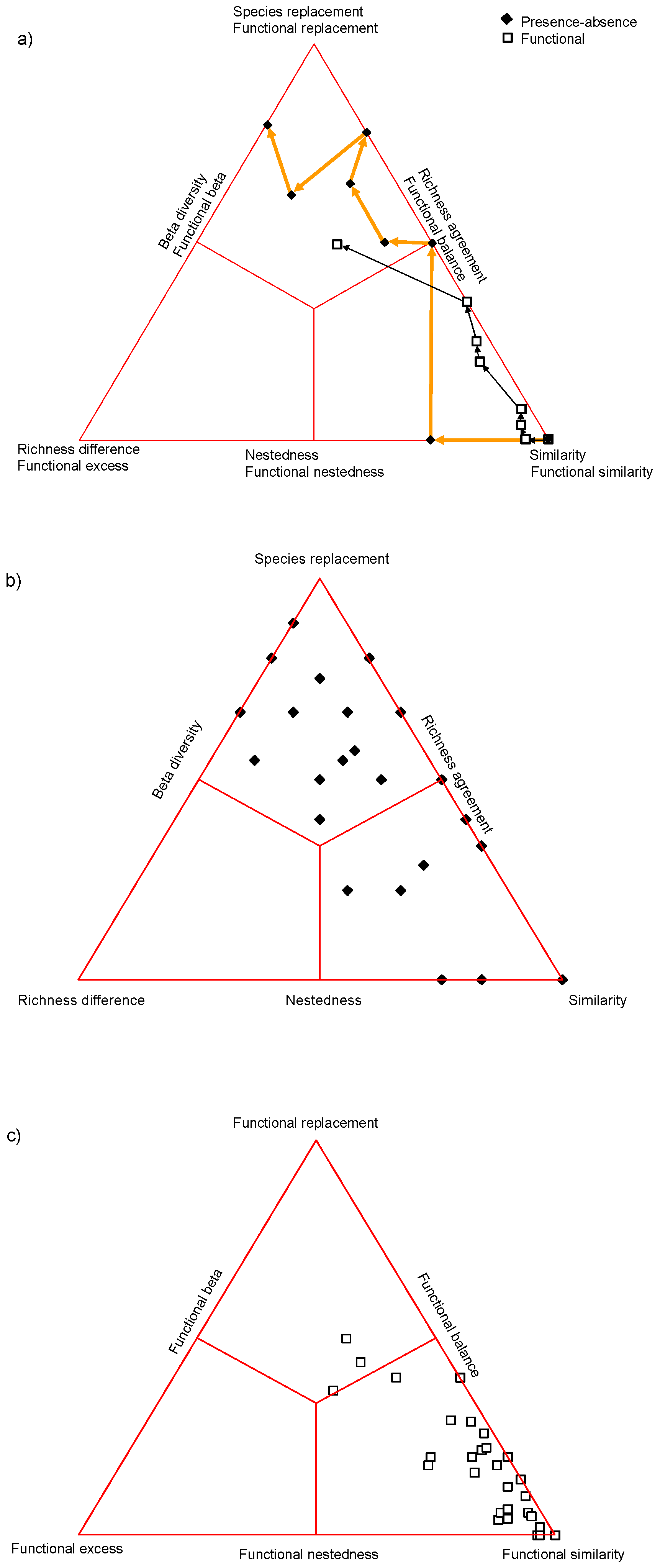
We refer to the sample data used by Ricotta et al. ([17], Table A1 in the Appendix A) in which a series of 9 plots was generated along a theoretical one-dimensional gradient, with 15 species responding to that gradient in a largely unimodal fashion. All plots were compared to the first plot using the Jaccard index based on species presence–absence and also considering a hypothetical functional distinctness matrix (see Ricotta et al. 2016b, Table A2 in the Appendix A) in the generalized Jaccard index. The two comparison series were illustrated in our previous paper in 3 graphical profile diagrams (Figure 1 in [17]) showing that the dissimilarity and species replacement/functional turnover almost always increased monotonically, while the changes of both richness difference and functional excess were completely irregular. Here we show the same changes as trajectories within the 2D simplex diagram (Figure 1a)—as an alternative and more compact illustration of the same process. Note that the last two points coincide, because the corresponding sites had identical species composition and therefore the same dissimilarity from plot 1. It is now obvious from the profile diagrams that taxon (species)-based dissimilarity changes more drastically than functional dissimilarity: both start from 0 (i.e., complete similarity of plot 1 with itself, lower right vertex) but only taxon based dissimilarity reaches the maximum (left edge of the triangle). For functional Jaccard index, the pair of the first and the penultimate plots does not reach maximum dissimilarity because the constituting species were not completely distinct functionally. Overall, the changes are more hectic for presence–absence than functional data, demonstrating the balancing effect of functional similarities among species. The trajectories also show lucidly the significance of each step along the series. Based on presence–absences, the move from plot 2 to 3 was the most drastic: plot 1 was completely nested in plot 2 (therefore the corresponding point is positioned exactly on the bottom side of the triangle) whereas plot 3 reached the same richness as plot 1 after 2 species replacements (hence the corresponding point is on the left side of the triangle). For functional data, the greatest change is in the step from plot 7 to 8 (and to 9): one species with low functional distinctness from the species of plot 1 disappears, whereas a new species, with high distinctness from the species of plot 1 appears here.
The simplex plots may be drawn for the entire data matrix to illustrate its overall structure—as originally suggested [6]. The differences between the species-based (Figure 1b) and functionality-based (Figure 1c) diagrams are considerable. There is high beta diversity for presence–absences (70.5%), most of the points lay within the species replacement (upper) third of the ternary plot. For functional data, however, the majority of points are positioned within the similarity (lower right) corner—beta diversity is lowered to 29.5%. Based on the average SDR fractions ( = 0.30, = 0.16, = 0.54 for the species-based simplex, = 0.71, = 0.09, = 0.2 for the functional), the normalized centroid distance, i.e., functional redundancy will be E’sf = 0.53/ = 0.37.
4.2. Actual Examples
Rank-based taxonomy follows in all cases a recent classification of plants by Chase and Reveal [24], which strongly relies upon the results of molecular systematics. At the order and family level the classification of angiosperms was refined according to the Angiosperm Phylogeny Group [25]. The phylogeny and the set of functional characters were derived more or less differently in each case study.
4.2.1. Grassland
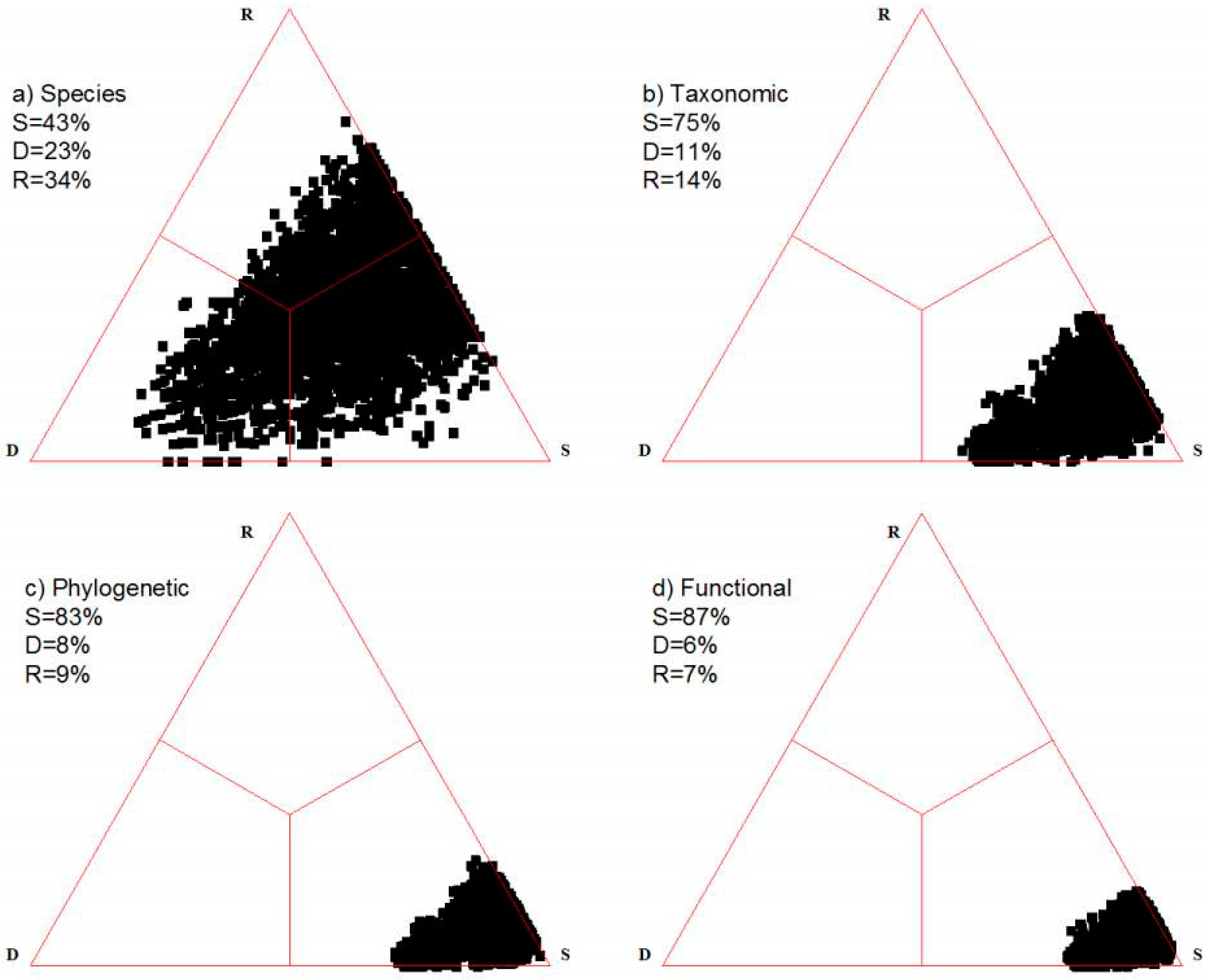
Presence–absence scores for 123 species in eighty 4 m × 4 m quadrats serve as the first actual example. Species richness ranges from 14 to 65 in the individual plots. These data were used previously in Podani and Miklós ([26], data given in their Electronic Supplement), for example. The vegetation of the study site is rock grassland on the southern, eastern and northern slopes and the top of Sas-hegy (Sas-hill), a nature reserve within the city limits of Budapest. The geology of the area is quite uniform; the bedrock is dolomite with some karstic formations on the surface. The soil, which varies in thickness depending mostly on slope angle, and the micro-climate which depends on aspect appear to be the major environmental factors affecting community composition. Physiognomy ranges from open rock grassland, where considerable surface remains bare, to closed grasslands in which plant cover reaches 100%. Floristically, the area is fairly homogeneous; there are many species distributed throughout. Figure 2a is the simplex diagram based on the decomposition of the traditional Jaccard index calculated for all quadrat pairs. The point cloud has a remarkable shape and arrangement along the contrast between the D vertex and the opposing R-S side, encountered most commonly in a comparative analysis of hundreds of published data sets [6]. Of the three components, similarity dominates, followed by replacement and richness difference while the sum of the latter two, i.e., beta diversity is higher than similarity (57%).
The ranks used here are the genus, family, order and superorder—the latter corresponding to the maximum taxonomic separation in the study site (six superorders, Lilianae, Ranunculanae, Rosanae, Caryophyllanae, Santalanae and Asteranae are represented). The number of orders is 19, divided into 33 families and then into 101 genera. The extended Jaccard index based on taxonomic separation of species produces the simplex diagram of Figure 2b. Similarity increases from 43% to 75% (that is, beta diversity decreases from 51% to 25%), causing the move of the entire point cloud towards the lower right (S) vertex. This shows that there is a high overall taxonomic similarity among the species of the study site; species absent from any plot are usually replaced by a taxonomically close relative in the other in pairwise comparisons.
The phylogeny, more specifically a cladogram for the 123 species was determined by the phylotools [27] and APE [28] programs. From the resulting tree, pairwise distance between any two species is obtained as the sum of branch lengths along the path between them. In the cladogram, the maximum separation occurs between the monocot and eudicot clades—this is because there are no gymnosperms and ferns in the study site, and the so-called “basal” dicot clades (e.g., Nymphaeales) are not represented either. The use of phylogenetic relationships increases even further the overall similarity of plots: it reaches 83%, which is also obvious from the visual examination of the simplex plot (Figure 2c). The fact that we have an 8% increase of similarity compared to the taxonomic simplex indicates that the current Linnaean system of plants suggested by Chase and Reveal [24] is fairly redundant compared to the phylogeny (i.e., a given phylogenetic distance is not always associated with the same level of taxonomic separation). Species of the Sas-hegy appear to have phylogenetic aggregation, species absent from a given plot can have a phylogenetically very close relative in that plot—thus decreasing between plot dissimilarity considerably. This means a high level of limiting similarity over the study area, which could be interpreted in terms of heterogeneity in microhabitats or limited competition thanks to high differences in species’ niches (assuming that niche traits have phylogenetic signal).
Finally, we examine the functional version the Jaccard index. The 123 species of the study area are described in terms of 17 functional variables representing several types of life form, growth form, ploidy level, pollination, leaf shape and seed characteristics (Table S1 in Supplementary Materials). As a result of incorporating functional information into the Jaccard index, overall between plot similarity increases even further, to 87%, so that the points in the triangle aggregate even more closely to the similarity vertex (Figure 2d). This is an indication of the considerably high functional agreement among the species of the study site.
The move of the point cloud along the series described above, that is, the monotonous decrease in beta diversity is reflected well by the distances of the centroids of point clouds from the centroid of the species based configuration (Table 2).
4.2.2. Primary Succession in the Alpine Zone
This data set contains 59 plots, each of about 25 m2 in size placed at the foreland of the Rutor Glacier, Aosta Valley, Italy [29,30]. The sampling design follows a space-for-time substitution model: each stage of the successional process is represented by moraine ridges of known age. In geological and climatic terms, the area is fairly homogeneous. The entire study site lies above the tree line, so that the vegetation is composed only of 45 herbaceous species. The original scores were expressed at an ordinal scale; we use here only p–a information. All data are available in Appendix S2 of Ricotta et al. ([30]). The species-based simplex diagram (Figure 3a) reflects a data structure with much higher beta diversity (thus, lower similarity) than in the grassland example above. The upper third section within the triangle is entirely covered by points, showing that species replacement is the dominating process during succession (51%) as opposed to species gains and losses (21%).
In the rank-based classification of the species, the same levels and the same six superorders appear as in the grassland example. These are subdivided into 11 orders, 15 families, and 37 genera. The simplex plot (Figure 3b) illustrates an increased concentration of points near the right edge, caused mostly by much decrease in replacement and increase in similarity. This largely reflects the situation that during succession many species are replaced by taxonomically close relatives.
The phylogeny of the 45 species (available in Appendix A of Ricotta et al. [31]) was extracted from the Daphne phylogeny [32], a dated phylogeny of a large European flora comprising most Italian species. In the cladogram, the first split separates monocots and eudicots. As in the grassland example, the use of phylogenetic information further increases the overall similarity of sample plots, resulting in a shift of the point cloud towards the S vertex (Figure 3c). That is, during succession species replacement is more pronounced in phylogenetic terms than in the rank-based taxonomy.
Each of the 45 species was given three scores to reflect their functionality in the community in terms of Grime’s plant strategy theory (C-competitors, S-stress tolerators, R-ruderals) such that their sum was 100 [29]. From the 3 × 45 functional data matrix obtained this way, the functional distinctness values were calculated using the Gower formula. In this case, since only metric information was incorporated, the formula reduces to the Manhattan distance calculated on variables each standardized by range. Given that for the three variables the actual minima were 0 twice, and 5 once, the results are very close to the dissimilarity matrix calculated using the Marczewski–Steinhaus index by Ricotta et al. [30]. The resulting simplex (Figure 3d) demonstrates extreme overall similarity achieved in this study (92%). It means that in the functional sense the sample sites include very similar floras along the entire successional sere. Overall, redundancy is higher in this study than in the grassland example above.
4.2.3. Coastal Marsh Vegetation
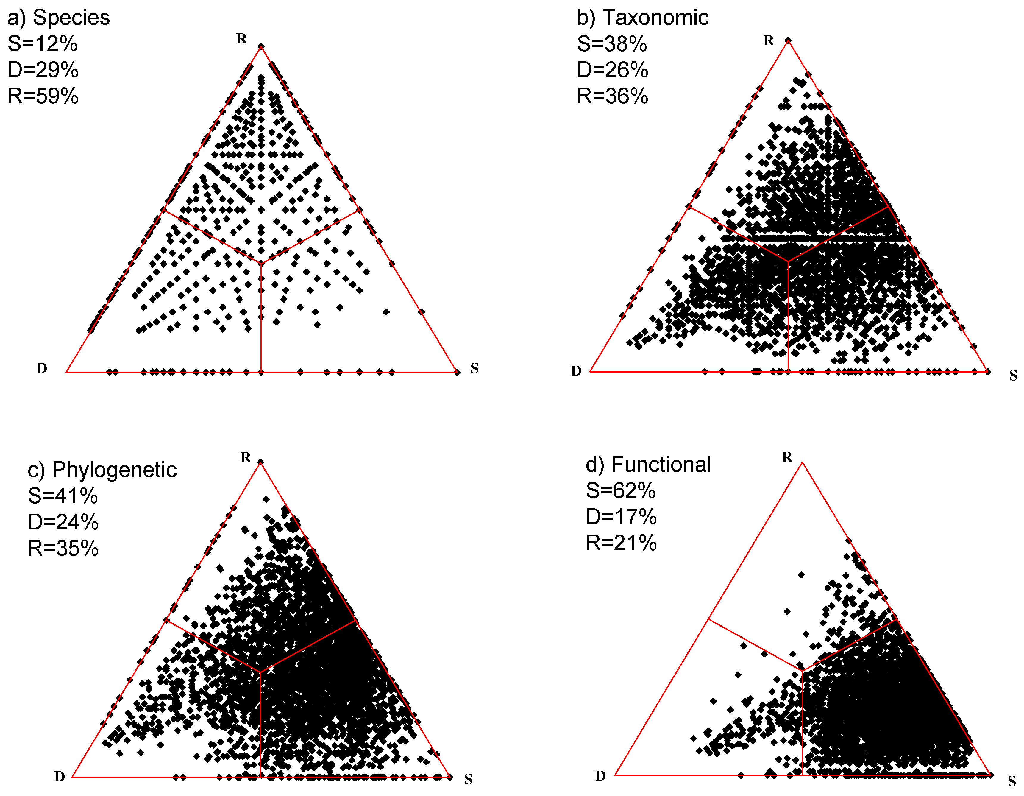
The study site from which this data set originates is the La Mafragh salt marsh plain near the Mediterranean coast in NE Algeria [33]. This plain is about 15,000 ha, within which 10,000 ha were surveyed. We analyzed the composition of 97 sites defined using a regular grid on the study area.
The elevation of the largest part of the area varies mostly from 1 to 4 m a.s.l. with the maximum of 6 m a.s.l. The entire area is furrowed by rivers, and constitutes a basin filled by alluvial and colluvial deposits. Soil composition varies: 77%, 4% and 1% of the sites are covered predominantly (>50%) by clay, sand, and silt, respectively. The soil of the remaining sites is heterogeneous and composed evenly of clay, sand and silt (about 33% each). The area is partially influenced by the effects of anthropogenic developments: drainage, river control, abandoned and active rice fields, extensive exploitation of natural fields as fodder and pasture (cattle breeding), an abandoned raised track. Dunes restrict water loss and the presence of an estuary (the Mafragh River) leads to sea water flooding during storms. The lowest parts are composed of large and small marshes with moderate to high levels of salinity. The highest levels of salinity occur near the sea where physical obstacles retain sea water after flooding, and far from the sea (12 km) in a clay-rich area with low elevation. Abundance and environmental data were collected by de Bélair [34], and we have now extended this data set by including bibliographical species traits and a phylogeny by Pavoine et al. [33] using the French Mediterranean floristic database BASECO [35] supplemented with information from many different articles and Floras (listed in Table 1 of Pavoine et al. [33] for the traits) and phylomatic software, the bladj algorithm [36], and dated nodes (mostly from Hedges and Kumar [37]) for the phylogeny (see Pavoine et al., [33] for details). A total of 56 species were observed.
The simplex plot calculated based on presence–absence data (Figure 4a) illustrates a very high level of beta diversity in which species replacement is the dominating component (59%). Overall similarity among the 97 sites is the lowest among the examples examined in this paper, reflecting extreme floristic heterogeneity of the study area. Plant species in La Mafragh have various origins. The effects of permanent water in the marsh all year long (even in summer) and the warm winters (no freezing temperatures) make this area a rare ecosystem, particularly in the Mediterranean Basin. These rare conditions at La Mafragh allow the unusual coexistence of subtropical and Euro-Siberian plant species. The extreme floristic heterogeneity may be explained by the high richness of the area and the high heterogeneity in terms of soil composition, elevation, and salinity.
In the rank-based classification, the 56 species belong to the same subclass, Magnoliidae, as in the grassland and glacier vegetation examples. These are subdivided into four superorders, 14 orders, 21 families and 51 genera. The simplex plot (Figure 4b) demonstrates the increased taxonomic heterogeneity of the salt marsh in comparison to the other two case studies of the present paper. That is, taxonomic beta diversity remains considerably high (62%). This is also reflected in that taxonomic redundancy is the lowest in the present study (0.25, see Table 2).
The use of phylogenetic distinctness in calculating the Jaccard index causes only a less conspicuous shift in the point configuration of the simplex diagram (Figure 4c), and the centroid moves also very little (by 0.02) from the centroid of the taxonomic configuration. This means that in this case the Linnaean system is a fairly good proxy of phylogeny.
For computing the functional simplex, we used, among the available ones, four traits that influenced community assembly in La Mafragh (see Appendix S3 in Pavoine et al. [33]). These included life cycle, pollination type, presence of spiky structures, and presence of hairy leaves. The functional distinctness values were calculated using the Gower formula as modified by Pavoine et al. [22] to incorporate binary and ordinal variables. As the simplex diagram demonstrates (Figure 4d), beta diversity (i.e., functional beta) further decreases but, nevertheless, the functional beta still remains by far the highest in this study (38% versus 13% for the Sas-hegy grassland data, and 8% for the alpine vegetation data). The extreme floristic heterogeneity is accompanied by high taxonomic, functional and phylogenetic heterogeneity. Notably, most species are distributed along a salinity gradient. In low salinity areas, Mediterranean dicotyledonous species that are seasonal, annual or biennial (numerous families) complete their cycle before the hot season. Many of them have hairy leaves which facilitate water retention and reflection of sun rays. Most of them are entomogamous and/or autogamous. In high salinity areas, co-occurring species are mainly salt-tolerant monocots from the Juncaceae and Cyperaceae and halophyte dicots from the Chenopodiaceae. Most of these species are perennial, anemogamous, with sometimes spiky structures but no hairy leaves. Overall, in the marshland we have a mosaic of very different environmental conditions in terms of soil composition and salinity, determining which species can persist in each site depending on their functional characteristics.
5. Discussion
It has been generally acknowledged in numerical ecology that the measurement of biodiversity in terms of the number of taxa (usually species) and their abundances provides only a one-sided view on community composition. Taxon-level analyses give equal weight to all constituting species thereby ignoring their evolutionary history [38] and ecological functionality [39]. Phylogenetic and functional information has been incorporated in calculating beta diversity in many ways, complemented with taxonomic indices which use the Linnaean hierarchy as a proxy to phylogeny when our knowledge on the latter is limited. In this methodology, coefficients that can be decomposed into additive fractions deserve particular attention because partitioning allows separating the effect of different underlying ecological drivers behind biodiversity.
Pioneering work in this regard is due to Baselga [5] who suggested to separate taxon-based beta diversity into turnover and nestedness-resultant components. His procedure was then modified to accommodate phylogenetic [40] and functional [39] information as well. An alternative partitioning scheme was suggested by Podani and Schmera [6] in which beta diversity was expressed as the sum of relative richness difference and relative species replacement as given by Equations (9) and (10). This framework was extended to phylogenetic and functional diversity, and potentially to taxonomic diversity as well by Cardoso et al. [14]. All these approaches are indirect because partitioning is made through some multivariate representation of the community and its constituting species. Leprieur et al. [40] and Cardoso et al. [14] converted the problem to the segmentation of species trees into overlapping edges for species that appear in both communities (their length giving the value of a for calculating dissimilarity) and tree segments unique to each community (their length giving b and c). Villéger et al. [39] used the convex hull approach in which the intersection of the two communities in the multivariate trait space corresponded to a, and their symmetric difference (sum of the two unique parts) to b + c. Then, the a, b, and c values were used to calculate beta diversity and its fractions using the Jaccard or Sorensen formula. Note that in these cases a, b, and c are not integers, therefore it is more logical mathematically to speak of the quantitative counterparts of these coefficients, namely the Marczewski–Steinhaus index and the Bray–Curtis index, respectively.
In the present paper, we proposed a method that goes back to the direct partitioning of the Jaccard index, thus requiring neither ordinations nor trees. This is possible via the generalized Jaccard index as suggested by Ricotta et al. [17]. In this, the values of b and c are decreased, while a increased, by the amount the differential species in either site are similar taxonomically, phylogenetically or functionally to the species of the other site. Then, similarity, richness difference (here: excess) and replacement are calculated using the newly obtained values A, B, and C (Equations (11)–(13)), which are continuous. Table 1 lists the terms we suggest for these components. An advantage of our approach is that the relationships among the components may be visualized by a 2D simplex diagram for all pairs of sites. Thus, the raw, taxon- (species-) based structure of the community may then be compared to its taxonomic, phylogenetic and functional alternatives.
The utility of the new method was demonstrated by three actual examples coming from different habitats (grassland, alpine meadow, and coastal marsh) for which we used the same taxonomic hierarchy and derived the phylogenies based on the most recent available information. Functionality was a bit more heterogeneous: in the grassland and the salt marsh examples, we had functional traits of mixed type directly describing meaningful ecological characteristics of species, while in the alpine meadow the C-S-R system was used with three synthetic variables for each species. It was not surprising, of course, that beta diversity decreased when similarities of differential species were considered, while it was unexpected that the rank order was always the same. As was obvious from the diagrams, as well as from the numerical results, beta diversity decreased, and similarity increased, in the following order: taxonomic, then phylogenetic and finally functional. Consistently with this, the centroid of the point cloud in the SDR triangle moved continuously towards the S corner in that order in all the three cases. That is, species are the least easily replaceable by taxonomic relatives (which is, of course, taxonomy-dependent). It was always easier to find phylogenetic relatives, and finally, the species were most readily replaceable by others based on their functional agreement. We do not want to derive far-reaching conclusions from this result, but nevertheless, we put forward the beta-redundancy hypothesis here that beta diversity decreases in ecological communities in the following order: taxon–taxonomic–phylogenetic–functional. The following comments and observations deserve attention here to judge the potential generality of this hypothesis:
- In fact this order cannot be evaluated whenever the measures applied to each level have different theoretical background. For example, Weinstein et al. [16] calculated taxon-based beta using the Sorensen index, and phylogenetic beta using the PhyloSor measure, so far so good, but functional beta was the mean nearest taxon distance calculated after PCA of the trait matrix. Tucker et al. [41] used the total branch length of the cladogram to measure phylogenetic beta and the convex hull for the functional beta in a simulation experiment. Most published research, like these, fails to satisfy this methodological consistency criterion and, therefore, their results cannot be compared with ours. Moreover, when the authors did care attention deliberately to commensurability [15], the results were in matrix form and remained unavailable for comparison.
- Functional diversity was the lowest (alpine meadow) when the number of functional variables was the lowest (3), raising the possibility that there is some direct relationship between these two.
- The choice of functional variables is subject to arbitrary decisions, while taxonomy and phylogeny do not depend on the authors’ wish. There is always the question if we indeed use the most meaningful set of functional characters in a given study.
- Taxonomy and phylogeny are constrained by their own hierarchy, neighbors or close relatives can only replace each other, whereas in terms of functionality two phylogenetically remote taxa may agree just as well, i.e., convergence increases the probability that one absent species may be replaced by another with similar functional traits.
- In theory, all the differential species in every comparison can be completely replaced regarding functionality, while this is impossible taxonomically and phylogenetically.
- Functional diversity as we measure here apparently correlates with environmental heterogeneity. Here it is the lowest in the alpine meadow vegetation (uniform habitat) followed by the grasslands also with fairly uniform habitat which differ only in exposition, and then comes the marshland which had the highest habitat heterogeneity;
- Thus, theoretically it may happen that environmental heterogeneity exceeds phylogenetic heterogeneity, i.e. when fairly related species were forced to adapt to extremely different environmental conditions and in such cases the beta redundancy hypothesis may not be true. In other words, the above order may be constrained by environmental heterogeneity and if we collect an extremely diverse sample (in which sites have nothing to do with each other).
- Our results do not support the view that phylogenetic beta often serves as a good surrogate to functional beta at the local scale; there was quite a big difference between them in homogeneous (alpine meadow) and heterogeneous (coastal marsh) environment as well. We agree with Losos [42] and Swenson et al. [43] who reached similar conclusions regarding the predictability of functional dissimilarity by phylogenetic dissimilarity.
Of course, further studies representing animals, woody vegetation, deserts, aquatic and microbial communities etc. are needed to confirm or reject the above hypothesis. Our study and the results raise further questions to be examined in the future, for example, regarding the effect of taxonomic decisions upon measuring taxonomic diversity—an important question in studies where phylogenetic information is limited.
All in all, our simplex analysis seems to offer valid comparisons among different studies. The methodology suggested here offers a possibility to evaluate four different facets of biodiversity as they appear in shaping community structure within the same methodological framework.
Supplementary Materials
The following are available online at https://www.mdpi.com/2227-7390/6/11/250/s1, Table S1: Functional data for 123 species in the Sas-hill study area. Excel file.
Author Contributions
Writing—original draft, J.P.; Writing—review & editing, S.P. and C.R.
Funding
Research of the first author was supported by Hungarian National Research Grant OTKA K128496.
Acknowledgments
Thanks are due to P. Csontos (Hungarian Academy of Sciences) for information on functional traits of species in the grassland example.
Conflicts of Interest
The authors declare they have no competing interests.
Appendix A

Table A1.
Artificial data set with 15 species (columns) and 9 sites (rows).
| 1 | 1 | 1 | 1 | 0 | 0 | 1 | 0 | 1 | 0 | 0 | 0 | 0 | 0 | 0 |
| 1 | 1 | 1 | 1 | 1 | 0 | 1 | 1 | 1 | 0 | 0 | 0 | 0 | 0 | 0 |
| 0 | 0 | 1 | 1 | 0 | 1 | 1 | 1 | 1 | 0 | 0 | 0 | 0 | 0 | 0 |
| 0 | 0 | 0 | 1 | 0 | 0 | 1 | 1 | 1 | 1 | 0 | 0 | 0 | 0 | 0 |
| 0 | 0 | 0 | 0 | 0 | 0 | 1 | 1 | 1 | 1 | 0 | 0 | 1 | 0 | 0 |
| 0 | 0 | 0 | 0 | 0 | 0 | 1 | 1 | 1 | 1 | 1 | 0 | 1 | 0 | 0 |
| 0 | 0 | 0 | 0 | 0 | 0 | 0 | 0 | 1 | 0 | 0 | 1 | 1 | 1 | 0 |
| 0 | 0 | 0 | 0 | 0 | 0 | 0 | 0 | 0 | 0 | 0 | 1 | 1 | 1 | 1 |
| 0 | 0 | 0 | 0 | 0 | 0 | 0 | 0 | 0 | 0 | 0 | 1 | 1 | 1 | 1 |
Table A2.
Artificial functional distinctness matrix for the 15 species in Table A1.
Table A2.
Artificial functional distinctness matrix for the 15 species in Table A1.
| 0 | 0 | 0.1 | 0.2 | 0.2 | 0.3 | 0.4 | 0.4 | 0.5 | 0.4 | 0.6 | 0.7 | 1 | 0.9 | 0.8 |
| 0 | 0 | 0.1 | 0.2 | 0.2 | 0.3 | 0.4 | 0.4 | 0.5 | 0.4 | 0.6 | 0.7 | 1 | 0.9 | 0.8 |
| 0.1 | 0.1 | 0 | 0.1 | 0.3 | 0.4 | 0.3 | 0.3 | 0.4 | 0.5 | 0.7 | 0.8 | 1 | 0.8 | 0.9 |
| 0.2 | 0.2 | 0.1 | 0 | 0.4 | 0.5 | 0.2 | 0.4 | 0.3 | 0.6 | 0.8 | 0.9 | 0.9 | 0.9 | 1 |
| 0.2 | 0.2 | 0.3 | 0.4 | 0 | 0.1 | 0.4 | 0.4 | 0.5 | 0.4 | 0.4 | 0.7 | 1 | 0.9 | 0.8 |
| 0.3 | 0.3 | 0.4 | 0.5 | 0.1 | 0 | 0.3 | 0.3 | 0.4 | 0.3 | 0.3 | 0.6 | 1 | 0.8 | 0.7 |
| 0.4 | 0.4 | 0.3 | 0.2 | 0.4 | 0.3 | 0 | 0.2 | 0.1 | 0.4 | 0.6 | 0.7 | 0.7 | 0.7 | 0.8 |
| 0.4 | 0.4 | 0.3 | 0.4 | 0.4 | 0.3 | 0.2 | 0 | 0.1 | 0.2 | 0.4 | 0.5 | 0.7 | 0.5 | 0.6 |
| 0.5 | 0.5 | 0.4 | 0.3 | 0.5 | 0.4 | 0.1 | 0.1 | 0 | 0.3 | 0.5 | 0.6 | 0.6 | 0.6 | 0.7 |
| 0.4 | 0.4 | 0.5 | 0.6 | 0.4 | 0.3 | 0.4 | 0.2 | 0.3 | 0 | 0.2 | 0.3 | 0.7 | 0.5 | 0.4 |
| 0.6 | 0.6 | 0.7 | 0.8 | 0.4 | 0.3 | 0.6 | 0.4 | 0.5 | 0.2 | 0 | 0.3 | 0.7 | 0.5 | 0.4 |
| 0.7 | 0.7 | 0.8 | 0.9 | 0.7 | 0.6 | 0.7 | 0.5 | 0.6 | 0.3 | 0.3 | 0 | 0.4 | 0.2 | 0.1 |
| 1 | 1 | 1 | 0.9 | 1 | 1 | 0.7 | 0.7 | 0.6 | 0.7 | 0.7 | 0.4 | 0 | 0.2 | 0.3 |
| 0.9 | 0.9 | 0.8 | 0.9 | 0.9 | 0.8 | 0.7 | 0.5 | 0.6 | 0.5 | 0.5 | 0.2 | 0.2 | 0 | 0.1 |
| 0.8 | 0.8 | 0.9 | 1 | 0.8 | 0.7 | 0.8 | 0.6 | 0.7 | 0.4 | 0.4 | 0.1 | 0.3 | 0.1 | 0 |
References
- Orlóci, L. Multivariate Analysis in Vegetation Research, 2nd ed.; Junk: The Hague, The Netherlands, 1978. [Google Scholar]
- Legendre, P.; Legendre, L. Numerical Ecology, 3rd ed.; Elsevier: Amsterdam, The Netherlands, 2012. [Google Scholar]
- Magurran, A.E. Measuring Biological Diversity; Blackwell Science: Oxford, UK, 2004. [Google Scholar]
- Baselga, A. Multiple site dissimilarity quantifies compositional heterogeneity among several sites, while average pairwise dissimilarity may be misleading. Ecography 2013, 36, 124–128. [Google Scholar] [CrossRef]
- Baselga, A. Partitioning the turnover and nestedness components of beta diversity. Glob. Ecol. Biogeogr. 2010, 19, 134–143. [Google Scholar] [CrossRef]
- Podani, J.; Schmera, D. A new conceptual and methodological framework for exploring and explaining pattern in presence–absence data. Oikos 2011, 120, 1625–1638. [Google Scholar] [CrossRef]
- Carvalho, J.C.; Cardoso, P.; Gomes, P. Determining the relative roles of species replacement and species richness differences in generating beta-diversity patterns. Glob. Ecol. Biogeogr. 2012, 21, 760–771. [Google Scholar] [CrossRef]
- Legendre, P. Interpreting the replacement and richness difference components of beta diversity. Glob. Ecol. Biogeogr. 2014, 23, 1324–1334. [Google Scholar] [CrossRef] [Green Version]
- Jaccard, P. Distribution de la flore alpine dans le bassin des Dranses et dans quelques régions voisines. Bulletin. Société Vaudoise Sci. Naturelles 1901, 37, 241–272. [Google Scholar]
- Warwick, R.M.; Clarke, K.R. New “biodiversity” measures reveal a decrease in taxonomic distinctness with increasing stress. Mar. Ecol. Prog. Ser. 1995, 129, 301–305. [Google Scholar] [CrossRef]
- Warwick, R.M.; Clarke, K.R. Taxonomic distinctness and environmental assessment. J. Appl. Ecol. 1998, 35, 532–543. [Google Scholar] [CrossRef] [Green Version]
- Pavoine, S.; Baguette, M.; Stevens, V.M.; Leibold, M.; Turlure, C.; Bonsall, M.B. Life history traits, but not phylogeny, drive compositional patterns in a butterfly metacommunity. Ecology 2014, 95, 3304–3313. [Google Scholar] [CrossRef] [Green Version]
- Gerhold, P.; Cahill, J.; Winter, M.; Bartish, I.V.; Prinzing, A. Phylogenetic patterns are not proxies of community assembly mechanisms (they are far better). Funct. Ecol. 2015, 29, 600–614. [Google Scholar] [CrossRef] [Green Version]
- Cardoso, P.; Rigal, F.; Carvalho, J.C.; Fortelius, M.; Borges, P.A.V.; Podani, J.; Schmera, D. Partitioning taxon, phylogenetic and functional beta diversity into replacement and richness difference components. J. Biogeogr. 2014, 41, 749–761. [Google Scholar] [CrossRef]
- Corbelli, J.M.; Zurita, G.A.; Filloy, J.; Galvis, J.P.; Vespa, N.I.; Bellocq, I. Integrating taxonomic, functional and phylogenetic beta diversities: Interactive effects with the biome and land use across taxa. PLoS ONE 2015, 10. [Google Scholar] [CrossRef] [PubMed]
- Weinstein, B.G.; Tinoco, B.; Parra, J.L.; Brown, L.M.; McGuire, J.A.; Stiles, F.G.; Graham, C.H. Taxonomic, phylogenetic, and trait beta diversity in South American hummingbirds. Am. Nat. 2014, 184, 211–224. [Google Scholar] [CrossRef] [PubMed]
- Ricotta, C.; Podani, J.; Pavoine, S. A family of functional dissimilarity measures for presence and absence data. Ecol. Evol. 2016, 6, 5383–5389. [Google Scholar] [CrossRef] [PubMed] [Green Version]
- Izsak, C.; Price, A.R.G. Measuring β-diversity using a taxonomic similarity index, and its relation to spatial scale. Mar. Ecol. Prog. Ser. 2001, 215, 69–77. [Google Scholar] [CrossRef]
- Carvalho, J.C.; Cardoso, P.; Borges, P.A.V.; Schmera, D.; Podani, J. Measuring fractions of beta diversity and their relationships to nestedness: A theoretical and empirical comparison of novel approaches. Oikos 2013, 122, 825–834. [Google Scholar] [CrossRef] [Green Version]
- Podani, J. Extending Gower’s general coefficient of similarity to ordinal characters. Taxon 1999, 48, 331–340. [Google Scholar] [CrossRef]
- Podani, J.; Schmera, D. On dendrogram-based measures of functional diversity. Oikos 2006, 115, 179–185. [Google Scholar] [CrossRef] [Green Version]
- Pavoine, S.; Vallet, J.; Dufour, A.-B.; Gacher, S.; Daniel, H. On the challenge of treating various types of variables: Application for improving the measurement of functional diversity. Oikos 2009, 118, 391–402. [Google Scholar] [CrossRef]
- Pavoine, S.; Marcon, E.; Ricotta, C. “Equivalent numbers” for species, phylogenetic, or functional diversity in a nested hierarchy of multiple scales. Meth. Ecol. Evol. 2016, 7, 1152–1163. [Google Scholar] [CrossRef]
- Chase, M.W.; Reveal, J.L. A phylogenetic classification of the land plants to accompany APG III. Bot. J. Linn. Soc. 2009, 161, 122–127. [Google Scholar] [CrossRef] [Green Version]
- Angiosperm Phylogeny Group. An update of the Angiosperm Phylogeny Group classification for the orders and families of flowering plants: APG IV. Bot. J. Linn. Soc. 2016, 181, 1–20. [Google Scholar] [CrossRef] [Green Version]
- Podani, J.; Miklós, I. Resemblance coefficients and the horseshoe effect in principal coordinates analysis. Ecology 2002, 83, 3331–3343. [Google Scholar] [CrossRef]
- Phylotools: Phylogenetic Tools for Eco-Phylogenetics; R package Version 0.1.2. Available online: https://cran.r-project.org/web/packages/phylotools/index.html (accessed on 12 November 2018).
- Paradis, E.; Claude, J.; Strimmer, K. APE: Analyses of phylogenetics and evolution in R language. Bioinformatics 2004, 20, 289–290. [Google Scholar] [CrossRef] [PubMed]
- Caccianiga, M.; Luzzaro, A.; Pierce, S.; Ceriani, R.M.; Cerabolini, B. The functional basis of a primary succession resolved by CSR classification. Oikos 2006, 112, 10–20. [Google Scholar] [CrossRef]
- Ricotta, C.; Luzzaro, A.; Pierce, S.; Ceriani, R.M.; Cerabolini, B. Measuring the functional redundancy of biological communities: A quantitative guide. Meth. Ecol. Evol. 2016, 7, 1386–1395. [Google Scholar] [CrossRef]
- Ricotta, C.; Bacaro, G.; Caccianiga, M.; Cerabolini, B.E.L.; Moretti, M. A classical measure of phylogenetic dissimilarity and its relationship with beta diversity. Basic Appl. Ecol. 2015, 16, 10–18. [Google Scholar] [CrossRef]
- Durka, W.; Michalski, S.G. Daphne: A dated phylogeny of a large European flora for phylogenetically informed ecological analyses. Ecology 2012, 93, 2297. [Google Scholar] [CrossRef]
- Pavoine, S.; Vela, E.; Gacher, S.; de Bélair, G.; Bonsall, M.B. Linking patterns in phylogeny, traits, abiotic variables and space: A novel approach to linking environmental filtering and plant community assembly. J. Ecol. 2011, 99, 165–175. [Google Scholar] [CrossRef]
- De Bélair, G. Biogéographie et Aménagement: La Plaine de La Mafragh (Annaba, Algérie). Ph.D. Thesis, Université Paul Valéry, Montpellier, France, 1981. [Google Scholar]
- Gachet, S.; Véla, E.; Tatoni, T. BASECO: A floristic and ecological database of Mediterranean French flora. Biodivers. Conserv. 2005, 14, 1023–1034. [Google Scholar] [CrossRef]
- Webb, C.O.; Ackerly, D.D.; Kembel, S.W. Phylocom: Software for the analysis of phylogenetic community structure and character evolution. Bioinformatics 2008, 24, 2098–2100. [Google Scholar] [CrossRef] [PubMed]
- Hedges, S.B.; Kumar, S. (Eds.) The Timetree of Life; Oxford University Press: Oxford, UK, 2009. [Google Scholar]
- Webb, C.O.; Ackerly, D.D.; McPeek, M.A.; Donoghue, M.J. Phylogenies and Community Ecology. Annu. Rev. Ecol. Syst. 2002, 33, 475–505. [Google Scholar] [CrossRef]
- Villéger, S.S.; Grenouillet, G.; Brosse, S. Decomposing functional beta-diversity reveals that low functional beta-diversity is driven by low functional turnover in European fish assemblages. Glob. Ecol. Biogeogr. 2013, 22, 671–681. [Google Scholar] [CrossRef]
- Leprieur, F.; Albouy, C.; De Bortoli, J.; Cowman, P.F.; Bellwood, D.R.; Mouillot, D. Quantifying phylogenetic beta diversity: Distinguishing between ‘true’ turnover of lineages and phylogenetic diversity gradients. PLoS ONE 2012, 7. [Google Scholar] [CrossRef]
- Tucker, C.M.; Davies, T.J.; Cadotte, M.W.; Pearse, W.D. On the relationship between phylogenetic diversity and trait diversity. Ecology 2018, 99, 1473–1479. [Google Scholar] [CrossRef] [PubMed]
- Losos, J.B. Phylogenetic niche conservatism, phylogenetic signal and the relationship between phylogenetic relatedness and ecological similarity among species. Ecol. Lett. 2008, 11, 995–1003. [Google Scholar] [CrossRef] [PubMed]
- Swenson, N.G.; Erickson, D.; Mi, X.; Bourg, N.A.; Forero-Montana, J.; Ge, X.; Howe, R.; Lake, J.K.; Liu, X.; Ma, K.; et al. Phylogenetic and functional alpha and beta diversity in temperate and tropical tree communities. Ecology 2012, 93. [Google Scholar] [CrossRef] [Green Version]
Figure 1.
Analysis of the sample data. (a) A SDR simplex plot for the decomposition of the generalized Jaccard index for functional components. The two trajectories reflect the comparison of the first site with itself and all other sites along the sequence (see text), (b) taxon- (species-) based simplex plot, (c) functional simplex. Note that points corresponding to different plot pairs may coincide if they are identical in species composition, such as the endpoints of the two trajectories in (a) (pertaining to plot pairs 1–8 and 1–9).

Figure 2.
Four simplex diagrams for the Sas-hegy grassland data. Percentage scores refer to the respective centroids multiplied by 100. (a) Species; (b) Taxonomic; (c) Phylogenetic; (d) Functional.
Figure 2.
Four simplex diagrams for the Sas-hegy grassland data. Percentage scores refer to the respective centroids multiplied by 100. (a) Species; (b) Taxonomic; (c) Phylogenetic; (d) Functional.

Figure 3.
Four simplex diagrams for the primary succession in the alpine zone. Percentage scores refer to the respective centroids multiplied by 100. (a) Species; (b) Taxonomic; (c) Phylogenetic; (d) Functional.
Figure 3.
Four simplex diagrams for the primary succession in the alpine zone. Percentage scores refer to the respective centroids multiplied by 100. (a) Species; (b) Taxonomic; (c) Phylogenetic; (d) Functional.

Figure 4.
Four simplex diagrams for the salt marsh data. Percentage scores refer to the respective centroids multiplied by 100. (a) Species; (b) Taxonomic; (c) Phylogenetic; (d) Functional.
Figure 4.
Four simplex diagrams for the salt marsh data. Percentage scores refer to the respective centroids multiplied by 100. (a) Species; (b) Taxonomic; (c) Phylogenetic; (d) Functional.

Table 1.
Components of the SDR simplex for traditional taxon-based presence–absence data and their modification according to taxonomic, phylogenetic and functional distinctness of species.
Table 1.
Components of the SDR simplex for traditional taxon-based presence–absence data and their modification according to taxonomic, phylogenetic and functional distinctness of species.
| Component | Taxon | Taxonomic | Phylogenetic | Functional |
|---|---|---|---|---|
| dij = 1 | 0 ≤ dij ≤ 1 | |||
| S | similarity | t. similarity | ph. similarity | f. similarity |
| D | richness difference | t. excess | ph. excess | f. excess |
| R | replacement | t. replacement | ph. replacement | f. replacement (turnover) |
| β = R + D = JAC | dissimilarity (pairwise beta diversity, species turnover) | t. dissimilarity (=t. beta) | ph. dissimilarity (ph. beta) | f. dissimilarity (f. beta) |
| G = R + S | richness agreement | t. balance | ph. balance | f. balance |
| N = D + S (S > 0) | nestedness | t. nestedness | ph. nestedness | f. nestedness |
Table 2.
Taxonomic, phylogenetic and functional redundancy, as expressed by normalized centroid distances (Equation (15)) from the species-based configuration, in the actual ecological examples.
Table 2.
Taxonomic, phylogenetic and functional redundancy, as expressed by normalized centroid distances (Equation (15)) from the species-based configuration, in the actual ecological examples.
| Case study | Taxonomic (E′st) | Phylogenetic (E′sp) | Functional (E′sf) |
|---|---|---|---|
| Grassland | 0.27 | 0.35 | 0.38 |
| Alpine meadow | 0.29 | 0.41 | 0.57 |
| Salt marsh | 0.25 | 0.27 | 0.44 |
© 2018 by the authors. Licensee MDPI, Basel, Switzerland. This article is an open access article distributed under the terms and conditions of the Creative Commons Attribution (CC BY) license (http://creativecommons.org/licenses/by/4.0/).
Share and Cite
MDPI and ACS Style
Podani, J.; Pavoine, S.; Ricotta, C. A Generalized Framework for Analyzing Taxonomic, Phylogenetic, and Functional Community Structure Based on Presence–Absence Data. Mathematics 2018, 6, 250. https://doi.org/10.3390/math6110250
AMA Style
Podani J, Pavoine S, Ricotta C. A Generalized Framework for Analyzing Taxonomic, Phylogenetic, and Functional Community Structure Based on Presence–Absence Data. Mathematics. 2018; 6(11):250. https://doi.org/10.3390/math6110250
Chicago/Turabian StylePodani, János, Sandrine Pavoine, and Carlo Ricotta. 2018. "A Generalized Framework for Analyzing Taxonomic, Phylogenetic, and Functional Community Structure Based on Presence–Absence Data" Mathematics 6, no. 11: 250. https://doi.org/10.3390/math6110250
Note that from the first issue of 2016, this journal uses article numbers instead of page numbers. See further details here.