
Selection of Optimal Magnets for Traction Motors to Prevent Demagnetization

1
MagWeb USA, Frisco, TX 75035, USA
2
MAGNA Powertrain GmbH, 2514 Traiskirchen, Austria
*
Author to whom correspondence should be addressed.
Machines 2021, 9(6), 124; https://doi.org/10.3390/machines9060124
Submission received: 20 May 2021
/
Revised: 15 June 2021
/
Accepted: 16 June 2021
/
Published: 20 June 2021
(This article belongs to the Section Vehicle Engineering)
Abstract
:Currently, permanent-magnet-type traction motors drive most electric vehicles. However, the potential demagnetization of magnets in these motors limits the performance of an electric vehicle. It is well known that during severe duty, the magnets are demagnetized if they operate beyond a ‘knee point’ in the B(H) curve. We show herein that the classic knee point definition can degrade a magnet by up to 4 grades. To prevent consequent excessive loss in performance, this paper defines the knee point k as the point of intersection of the B(H) curve and a parallel line that limits the reduction in its residual flux density to 1%. We show that operating above such a knee point will not be demagnetizing the magnets. It will also prevent a magnet from degenerating to a lower grade. The flux density at such a knee point, termed demag flux density, characterizes the onset of demagnetization. It rightly reflects the value of a magnet, so can be used as a basis to price the magnets. Including such knee points in the purchase specifications also helps avoid the penalty of getting the performance of a low-grade magnet out of a high-grade magnet. It also facilitates an accurate demagnetization analysis of traction motors in the worst-case conditions.
1. Introduction
At present, 80 to 90% of electric vehicles sold globally use permanent magnet (PM) type traction motors [1]. Rare-earth magnets are a critical but expensive component of all such applications. However, these magnets carry a demagnetization risk which can cause a permanent loss in the performance of the electric vehicle. Vehicle manufacturers recently recognized that such an irreversible demagnetization fault (IDF) is a major risk factor of PM motors [2,3,4]. This Achilles heel of PM motors prevents them from competing with the induction motors for applications such as pumps, fans, and compressors [5]. Therefore, engineers constantly seek approaches that minimize the demagnetization risk. This risk can occur during severe duties such as short-circuit, rapid acceleration from 0 to 60 mph, hill climbing, etc. Such worst cases or severe duties apply large demagnetizing fields on the magnets. Large fields that are beyond the capability of a magnet can cause excessive demagnetization. Thus, there is a fundamental need to define a proper metric to judge as to when an unacceptably large demagnetization occurs. In traction motors, this occurs at high temperatures, so it is sometimes called heat resistance.
The magnetic characteristics of a magnet are described by plots that show the variation of flux density B or J [tesla] with demagnetizing field H [kA/m]. They can be represented as a magnetic flux density B(H) curve or a ferric flux density J(H) curve. J is also known as polarization or intrinsic flux density. It is the magnetic flux density B less vacuum flux density µoH where μo = 4π∙10−7 [N/A2] is the permeability of vacuum(J ≡ B − µoH).
Both curves have a ‘knee’ that joins a reversible line segment smoothly with an irreversible segment. On a J(H) curve, the knee will fall in the 2nd quadrant. On a B(H) curve, for traction motors that operate at elevated temperatures, the knee will also fall in the 2nd quadrant. For others, it can fall in the 3rd quadrant, so it will require additional data. The knee signifies the transition to demagnetization.
A specific ‘knee point’ within a knee demarcates the change in the behavior of the magnet from a reversible state to an irreversibly demagnetized state. When a magnet operates above the ‘knee point’, it will return reversibly to its initial state, with no reduction in the residual flux density Br [6,7,8]. However, operating below the knee point will cause it to return along a parallel path which will reduce the residual flux density to a smaller value Br′. This reduction in residual flux density δBr = Br − Br′ is known as a demagnetization loss, irreversible loss, or simply loss.
Such reduction in Br requires more current to generate the same torque. This increases the copper loss, which increases the magnet temperature further, which in turn degrades the magnet more. The resulting vicious circle can cause a significant loss in the performance of the electric vehicle.
An unacceptably large demagnetization loss will push the operating point below the knee point, thereby causing an unacceptably large permanent reduction in the flux-producing capability of the magnet [8,9]. Since the flux density falls sharply as a waterfall beyond the knee, a minute increase in the demagnetizing field can drastically reduce the performance of a traction motor [9,10]. This can reduce the service life of the electric vehicle. In addition, replacing a demagnetized magnet in an electric vehicle is labor-intensive and very expensive. The resulting large downtime can even dissuade a consumer from using electric vehicles altogether.
The knee point thus plays a critical role in limiting the performance of an electric vehicle. It also characterizes IDF. Therefore, knowledge of the precise position of the knee point is critical for the selection of magnets in traction motors and to prevent IDF. The primary purpose of this paper is therefore to develop a well-defined method to locate the position of the knee point of a magnet on its B(H) curve.
At present, different engineering communities seem to have different views of the location of the knee point. To distinguish them, we label them as:
- Classic knee point K;
- Knee endpoint k′.
Classic knee point K—The magnet material engineers (who develop/test magnets) use the J(H) curve to define the classic knee point K. They define K as the point on the J(H) curve that permits 10% Br demagnetization loss. (In the 1960s, up to 20% loss was considered acceptable [11,12]). Their metric for demagnetization is the respective field HK.
Historically, in the 1980s, material engineers used such HK to indicate magnets with fewer defects [13,14]. A J(H) curve that is closest to the largest rectangle Br HcJ is deemed to have the least defects (HcJ = coercivity on the J(H) curve). They used the ‘loop squareness’ HK/HcJ [15,16] as a metric to develop better compositions that yielded magnets with the fewest defects [17,18].
In the 1990s, they used the same HK to define the acceptable limit on the demagnetization loss [19,20,21]. Initially, they presumed that the linear segment of J(H) of rare-earths to be nearly horizontal. Therefore, they defined the classic knee point K as the point on the J(H) curve where it intersects a horizontal line that passes through the 0.9∙Br point [22,23,24]. However, the linear segment is slightly inclined [25,26]. Therefore, later Gaster [27,28] redefined it as the point on the J(H) where it intersects a parallel inclined line that passes through the 0.9∙Br point. Both definitions indicate that the material engineers considered the 10% reduction in Br to be acceptable.
Material engineers widely consider that coercivity HcJ is the metric for the demagnetizability of a magnet. However, in 2008, Trout [29] wrote that the ‘(classic) knee point field HK may be a better figure of merit’ (than coercivity HcJ) or better metric for the onset of demagnetization. Since then, all commercial B(H) measurement systems are programmed to list this HK [30,31,32,33]. Currently, manufacturers use this HK in purchase specifications as a basis to negotiate the price of the magnets. However, over the past 10 years, tremendous improvements enabled the manufacturers to make superior magnets to tighter tolerances. Modern magnets, therefore, require a better metric with a tighter tolerance than the 10% loss allowed by HK.
Knee endpoint k′—The motor design engineers (who select and size the magnets for traction motors), on the other hand, rely on the Maxwell laws-based magnetic field software for the detailed design of traction motors [34,35,36]. Such software uses the B(H) curve rather than the J(H) curve. Therefore, these engineers rely on the B(H) curve to define the knee endpoint k′. They define it as one where the knee on the B(H) curve starts deviating from a straight line to a curve [37].
Their metric for demagnetization is the knee endpoint flux density Bk′. Motors subject the magnets to nonuniform fields, so the demagnetized volumes (where the flux density is less than the knee endpoint flux density Bk′) are local at the edges or center of magnets. The motor design engineers rely on Bk′ to estimate the demagnetized volume fraction Vd [38,39,40,41,42], which is then used to limit the loss in performance caused by the demagnetization of the magnets.
1.1. Difference between K, k′
The following examples illustrate that these prior-art knee points K, k′ differ significantly.
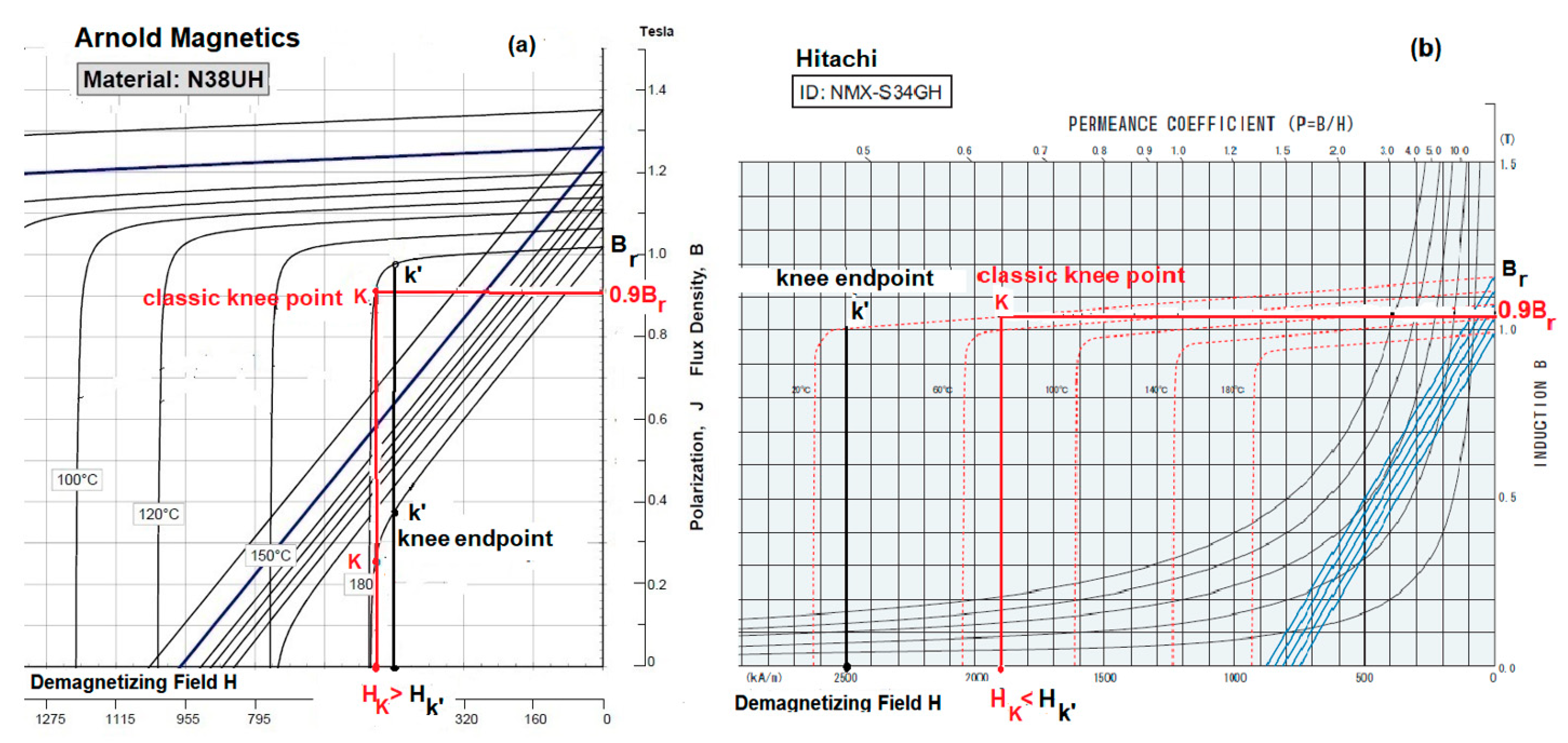
Figure 1a displays the demagnetization curves for Arnold’s N38UH grade at 180 °C [43]. It shows that the classic knee point K lies close to the irreversible segment, while the knee endpoint k′ lies close to its reversible segment. Specifically, the classic knee point flux density BK (0.25 T) is ~30% lower than the knee endpoint flux density Bk′ (0.37 T). It shows that the classic knee point field HK (−517.2 kA/m) is numerically 9% higher than that Hk′ at the knee endpoint (−475 kA/m).
As indicated earlier, at present engineers tie the price of the magnet to the field HK at the classic knee point. The higher this HK, the higher the price. However, Figure 1a demonstrates that, by specifying HK as the basis to price magnets, a buyer is paying a significant, but spurious 9% higher price for a magnet.
Figure 1b displays the demagnetization curves for Hitachi’s NMX-N34GH [44]. It shows that (for the 20 °C curves) the classic knee point K lies far inside the reversible segment, while the knee endpoint k′ lies close to the knee. Moreover, it shows that the classic knee point field HK (−1900 kA/m) is 30% (numerically) smaller than the knee endpoint field Hk′ (−2500 kA/m).
Figure 2 displays Innuovo’s N48UH at 180 °C [45]. As shown, the manufacturer lists the classic knee point field HK as −6.583 kOe (= −524 kA/m). However, its knee endpoint field Hk′ of −495.5 kA/m is 5.4% lower. This again demonstrates that using the classic knee point K to price magnets, a buyer is paying a significant, but spurious 5.4% higher cost for the magnet.
This plot also shows that its classic knee point K lies in the irreversible waterfall segment. Therefore, even a minute reduction in H will cause the flux density to fall sharply, thereby resulting in severe demagnetization. Moreover, it shows that its 0.32 T classic knee point flux density BK is 40% lower than the 0.45 T knee endpoint flux density Bk′.
All these examples confirm that the classic knee point K does not adequately represent the onset of demagnetization or value of a magnet. Moreover, it can be significantly different from the knee endpoint k′. So, from now onwards, we focus on the knee endpoint as it signals the onset of demagnetization better.
1.2. Manual Method to Locate k′
At present, a precise method to locate k′ is not available. The motor designers locate the knee endpoint k′ on a B(H) curve by a manual method, i.e., visually judging where the straight-line possibly ‘ends’ [46,47,48,49,50]. However, where exactly the knee ‘ends’ depends on the intuitive judgment of the person who picks it. For example, in Hitachi’s NMX-36EH at 180 °C, Choi [39] picked 0.14 T as the knee endpoint. However, actually, it is ~0.2 T—a 25% error.
Figure 3 shows that, for the HPMG N42UH grade at 150 °C [51], one engineer may pick point k1’, while another may pick point k2’. However, their flux densities are 0.21 and 0.31 T, respectively—a 50% error. These examples illustrate that the manual method of locating the knee endpoint k′ is imprecise and prone to significant errors.
1.3. Other Prior Methods to Locate k′
To define the starting point of demagnetization more precisely, over the past 20 years, several experts strived to devise various non-manual methods, but they fell short of expectations as discussed below.
By fitting a single model. These methods fit the entire B(H) data to a simple function, such as a hyperbola [52], arctan, tanh [53,54,55,56,57], coth [8], exponential [56], polynomial [58], or splines [59]. Over the past century, scores of attempts have been made to model the B(H) curves accurately [60]. However, most B(H) models are known to suffer from significant errors [59,61,62]. In addition, Peng [10] found that the k′ predicted by the tanh model differs significantly from that of tests. Moreover, fitting a single model does not locate k′ anyway. Due to all these considerations, the single model methods have not gained traction.
By fitting two models. These methods split the data into several segments. It fits one segment of data to a ‘straight-line model’ function and another segment to a ‘knee model’ function. Then, it determines k′ as the point of intersection of both. Several experts have employed diverse knee-models, e.g., arc of circle [61], exponential [6,7,62,63] or rational fraction [64]. However, the knee is so narrow that one usually can capture 2 to 4 data points at most [41]. Hence, fitting a knee model to so few data points can result in large errors [6,7]. For example, the Neo Grade 3512 at 160 °C, [7] showed that fitting the exponent model resulted in a 30% error. Therefore, these methods have also not gained traction.
Therefore, this prior-art review indicates so far that there has been no satisfactory method that can determine the knee endpoint precisely [65]. Thus, there is still a need to develop a method to precisely locate this critical point, called simply knee point k from now onwards. To achieve this, we first introduce the concept of degeneration.
2. Knee Point k
Degeneration is the phenomenon in which a higher grade magnet gets so demagnetized during the operation that its residual flux density degrades to that of a lower grade magnet. Once degenerated, a high-grade magnet behaves as a lower-grade magnet over its entire life. As a result, a degenerated magnet reduces the torque capacity of the motor permanently, thereby causing severe degradation of the performance of an electric vehicle forever.
Higher-grade magnets are very expensive. Their degeneration means that the extra dollars spent in buying the higher grade are wasted—it does not deliver the superior performance expected from the higher grade. To avoid such waste of money, one must make every effort to prevent degeneration.
To this end, we propose herein the knee point k as the point which prevents a magnet from degenerating to a lower grade. Operating above such knee point k will prevent an expensive high-grade from delivering the performance of a lower-grade magnet. We detail below an optimal method to determine this knee point k.
2.1. Offset Method
It is well known that, for metals, the stress-strain curve comprises linear (elastic) and nonlinear (inelastic) segments. A century ago, engineers faced the challenge of defining the ‘knee point’ of metals that demarcates the inelastic segment. They resolved it by creating the offset method. As shown in Figure 4b, this method defines a yield point Y as the point of intersection of the stress-strain curve and a parallel straight-line that is offset by a small but acceptable 0.2% strain. Yield strength is the stress at such yield point Y. The stress-strain curve above Y demarcates the inelastic segment.
In 1924, ASTM adopted this as the standard method to compute the yield strength. It codified this method in its Standard E8 [66]. Such a codified offset method is now universally used to quantify the strength of steels. Over the past 100 years, engineers relied on it to protect thousands of bridges and buildings against the inelastic behavior of steel.
Figure 4a shows that the B(H) curve of magnets is strikingly similar to the stress-strain curve of metals shown in Figure 4b. The offset method—which was used for years to protect against the yielding of metals—thus can also be used to protect against the demagnetization of magnets.
We define the knee point k as the point of intersection of the B(H) curve and a parallel straight-line that is offset by a small but acceptable demagnetization loss. To define it precisely, one has to specify as to what is an acceptable loss. As already indicated, the return path reduces the magnet’s residual flux density from Br to a smaller Br′. The reduction δBr = Br − Br′ is called demagnetization loss. Alternately, we reformulate it as offset x = δBr/Br (expressed as a percentage). Then, defining k amounts to specifying x.
2.2. Options for Offset x
Figure 4a displays knee point k as well as all prior-art knee points K, k′, and D (not to scale). We demonstrate herein how prior-art definitions of knee point are inadequate in protecting magnets against degeneration.
- 10% offset (K). This classic knee point K was proposed in the 1990s by magnet material engineers [20] as one that tolerates 10% Br loss. However, consider the N40UH grade with Br of 1.29 T. A 10% loss reduces it to Br′ of 1.16 T. Table 1 below shows that this is the Br for N33UH, which is three grades below N40UH. Thus, operating at the classic knee point K degenerates a magnet forever to a lower grade, so is unacceptable.
- 5% offset (D). This demagnetization point D was suggested in IEC 60404-8-1 [25,67] as one that tolerates 5% Br loss. However, consider the N50H magnet with Br of 1.40 T. A 5% loss reduces it to Br′ of 1.33 T. Table 1 shows that this is the Br for N42H, which is three grades below N50H. Thus, operating at the demag point D degenerates a magnet forever to a lower grade, so is unacceptable.
- 2% offset. This does not degenerate some magnets (for example, it reduces the 1.25 T Br of N35UH to 1.226 T. It is larger than the 1.15 T Br for a lower grade N33UH. Therefore, it will not degenerate this magnet). However, consider N52H with Br of 1.42 T Br. The 2% loss reduces it to Br′ of 1.39 T. This is Br for N50H, which is one grade below N52H. Thus, operating at this 2% loss the knee point can degenerate some magnets forever to a lower grade, so is unacceptable.
- 0.5% offset. This also does not degenerate a magnet, so it may seem to be acceptable. However, for N28EH with Br of 1.05 T, it amounts to 0.005 T, which is close to the measurement noise floor. However, at present, manufacturing a grade to such tight tolerances is nearly impossible. Specifying such tight tolerance will only increase their cost. Furthermore, tests by Allcock [68] revealed that most magnets suffer from a 0.4% Br long-term irreversible loss (LTIL). Therefore, specifying a 0.5% offset is unacceptable.
2.3. Rationale for 1% Offset
In this section, we present additional rationale to show that a 1% offset is the best option to define the knee point.
2.4. Grade Spacing
The standards subdivide the Neo magnets into about 10 grades. The Br of the lowest/highest grade N28/N55 is 1/1.5 T. Therefore, as one changes from the lowest grade to the highest, Br increases by 0.5 T. Since 10 grades fit into this 0.5 T span, they are spaced at about 0.05 T.
Table 1 below shows the spacing of conventional grades in greater detail. (It excludes the recent dysprosium-free ‘case hardened’ magnets which concentrate neodymium on the surface and refine the grain to reduce cost [69]). It shows that the grades in the 30–40 MGOe range are spaced at 0.05 T, while those in the 40–54 MGOe range are spaced at ~0.02 T. Thus, the smallest grade spacing is 0.02 T.
Therefore, to prevent a magnet from degenerating to a lower grade, the x% loss must be smaller than this smallest grade spacing of 0.02 T. Note that 0.02 T is 1.3% (~1%) of the largest Br of 1.5 T. Therefore, x = 1% offset is the best option to define the knee point k that prevents degeneration of a magnet to a lower grade.
2.5. Example
Figure 5a shows the B(H) curve and the return path (blue line) of grade N50H at its knee point k. In it, the red dotted line refers to the B(H) curve of the next lower grade N48H. It shows that the blue line is above the red dotted line. This indicates that, during the return path, the N50H residual flux density reduces from Br of 1.247 T to Br′ of 1.234 T. However, this is still greater than the 1.222 T residual flux density of the lower grade N48H. This establishes that operating a magnet up to its knee point k will not degenerate it to a lower grade.
Figure 5b shows the B(H) curve and the return path (blue line) of the same grade N50H, but now operating at its classic knee point K. In it, the red dotted line refers to the B(H) curve of N40H, which is four grades lower. It shows that the return blue line is below the red dotted line. This indicates that, during the return path, the N50H residual flux density now reduces from Br of 1.247 T to Br′ of 1.122 T. This is less than the 1.134 T residual flux density of N40H. This establishes that operating a magnet up to its classic knee point K will degenerate it to a lower grade.
3. Demag Flux Density
To prevent confusion, we rename the flux density Bk at the knee point k as the demagnetization flux density or simply demag flux density herein. Bk signals the onset of excessive demagnetization of magnets. It is similar to that of yield strength σy—which signals the onset of plastic or yielding of metals. Therefore, it is a key property of magnets.
Figure 6 shows a simplified representation of the demagnetization curves of a magnet (for Arnold’s N52M grade) [70]. It highlights that the residual flux density Br and the demag flux density Bk define the usable segment (green) of a magnet. It also shows that, with increasing temperature, Bk increases sharply while Br decreases mildly. Therefore, the rate at which a magnet’s usable range narrows with temperature is defined more by Bk than Br. This confirms that Bk is a key property of the magnet. Such a clutter-free demagnetization plot often provides a better insight as to how temperature impacts the usable range (conventional demagnetization curves cluster B(H) curves with J(H) curves, obscuring the usable range, see Figure 1, Figure 2 and Figure 3).
At present, all manufacturers of steel list the yield strength of all metals they produce. Similarly, it is hoped that all manufacturers of magnets will list the demag flux density Bk for their magnets. Just as the ASTM E8 spec helped widespread use of ‘yield strength’ σy, incorporating the ‘demag flux density’ Bk into international standards will enable its widespread use.
The key properties (Br, Bk) characterize the torque capability and heat resistance of the magnet, respectively. These metrics are valued by a motor designer. Therefore, they form the optimal cost basis for magnets.
Currently, engineers manually use the read Bk′ to compute the demagnetized volume fraction. However, as already shown, such manually read values can be imprecise. Instead, using the demag flux density Bk determined by the 1% offset method proposed herein will avoid such errors, resulting in more precise demagnetized volume fractions.
The demag flux density definition presented herein helps designers find an optimum tradeoff between performance degradation and the cost of the magnet. It is a better cost metric than HK (as B changes more rapidly than H in the knee). The eDrive systems by Magna Motors utilize it in their design, thereby resulting in a less expensive and more reliable drive system for future transportation mass market.
Recently, a new and comprehensive magnet property database by Rao [70] listed the coordinates (Hk, Bk) of the knee point k for all magnets produced worldwide. The demag flux density Bk included therein simplifies the task of accurate estimation of demagnetized volume fractions to limit performance degradation of electric vehicles.
The demag flux density maps presented in the next section allow one to examine how Bk varies with temperature and grade. This, in turn, shortens the process of selection of an optimal magnet that meets specific severe-duty performance requirements of electric vehicles.
4. Demag Flux Density Map
A demag flux density map displays the demag flux density Bk of all grades and temperatures. Figure 7 shows such a map for a specific manufacturer, over 120 to 180 °C. The grade corresponding to a point can be read off from Table 1. For example, the N33M-N52M curve has 9 points ranging from N33M to N52M, the 7th point refers to N48M, and its Bk at 120 and 150 °C is 0.7 and 0.85 T. Note that some curves are non-monotonic. This may be due to irregular grade spacing, inherent measurement noise, manufacturer variations, etc., which will be investigated in the future.
Such a plot can be used to determine the demag flux density offered by any grade at a specific temperature of interest. For example, it shows that N30SH offers a demag flux density of 0.32 T at 150 °C. It shows that a typical 0.7 T Bk requirement is met by the N48M grade at 120 °C or the N35M grade at 150 °C.
Such a plot can also be used to reduce the cost of magnets. For example, it shows that, by reducing the magnet temperature from 180 to 150 °C, one can replace an expensive N42UH grade with a less expensive N35SH grade. Both magnets have the demag flux density Bk of 0.38 T, which indicates that both deliver the same severe-duty performance. Therefore, this plot demonstrates how cooling a magnet can save significant costs of magnets.
5. Conclusions
It is well known that, at high temperatures, rare earth magnets will be demagnetized excessively if operated below a knee point on the B(H) curve. In this paper, we define the knee point k as one where the B(H) curve intersects with a parallel line that is offset by 1% Br. We showed herein that operating above such knee point k protects it from degenerating to a lower grade forever. The paper, therefore, recommends using this newly defined knee point k to prevent the degradation of magnets to a lower grade when simulating the severe-duty short circuit performance of traction motors. Data on this knee point k are available in the comprehensive PMAG database recently developed by MagWeb.
The respective demag flux density Bk is a key property of a magnet that signals the onset of excessive demagnetization. Listing it by manufacturers or incorporating it into international standards will help engineers better protect the magnets from degrading to a lower grade during the operation. Moreover, it helps them discover the right manufacturer who offers a better grade (with an optimal demag flux density Bk) for their application and cost reference. This helps in the selection of optimal magnets for traction motors in electric vehicles.
At present, the classic knee point field HK of a magnet (on a J(H) curve where a magnet can lose 10% Br) is popularly used to negotiate the price of the magnets. This paper, however, shows that this metric can overprice a magnet. Instead, it shows that the demag flux density Bk of a magnet (at the operating temperature) is a better cost metric as it prevents a magnet from degenerating to a lower grade. Using Bk rather than HK (to price the magnets) would be a milestone for future procurement strategies and the specification of magnets for traction motors in electric vehicles.
Author Contributions
Conceptualization, D.R.; methodology, M.B.; validation, M.B.; formal analysis, D.R.; investigation, D.R.; resources, D.R. writing—original draft preparation, D.R.; writing—review and editing, M.B.; visualization, supervision and project administration, D.R.; All authors have read and agreed to the published version of the manuscript.
Funding
This research received no external funding in conducting this research.
Institutional Review Board Statement
Not applicable.
Informed Consent Statement
Not applicable.
Data Availability Statement
Not applicable.
Conflicts of Interest
The authors declare no conflict of interest.
References
- Castilloux, R. Spotlight on Dysprosium. p. 25. Available online: https://www.adamasintel.com/spotlight-on-dysprosium/ (accessed on 20 February 2020).
- Lombardo, T. How to ensure EV traction motor magnets aren’t pushed beyond their operating limits. Charged 2020, 49, 3. [Google Scholar]
- Ullah, Z.; Hur, J. A comprehensive review of winding short circuit fault and irreversible demagnetization fault detection in PM type machines. Energies 2018, 11, 3309. [Google Scholar] [CrossRef] [Green Version]
- Islam, M.Z.; Arafat, A.; Bonthu, S.S.R.; Choi, S. Design of a Robust Five-Phase Ferrite-Assisted Synchronous Reluctance Motor With Low Demagnetization and Mechanical Deformation. IEEE Trans. Energy Convers. 2018, 34, 722–730. [Google Scholar] [CrossRef]
- Adly, A.; Huzayyin, A. The impact of demagnetization on the feasibility of permanent magnet synchronous motors in industry applications. J. Adv. Res. 2019, 17, 103–108. [Google Scholar] [CrossRef] [PubMed]
- Hamidizadeh, S.; Alatawneh, N.; Chromik, R.R.; Lowther, D.A. Comparison of different demagnetization models of permanent magnet in machines for electric vehicle application. IEEE Trans. Magn. 2016, 52, 1–4. [Google Scholar] [CrossRef]
- Hamidizadeh, S. Study of Magnetic Properties and Demagnetization Models of Permanent Magnets for Electric Vehicles Application; McGill University Libraries: Montreal, QC, Canada, 2016. [Google Scholar]
- Campbell, P. Permanent Magnet Materials and Their Application; Cambridge University Press: Cambridge, UK, 1996. [Google Scholar]
- Xiong, H.; Zhang, J.; Degner, M.W.; Rong, C.; Liang, F.; Li, W. Permanent magnet demagnetization test fixture design and validation. In Proceedings of the 2015 IEEE Energy Conversion Congress and Exposition, Montreal, QC, Canada, 20–24 September 2015; pp. 3914–3921. [Google Scholar]
- Peng, P.; Zhang, J.; Li, W.; Leonardi, F.; Rong, C.; Degner, M.W.; Liang, F.; Zhu, L. Temperature-Dependent Demagnetization of Nd-Fe-B Magnets for Electrified Vehicles. In Proceedings of the 2019 IEEE International Electric Machines & Drives Conference (IEMDC), San Diego, CA, USA, 12–15 May 2019; pp. 2056–2062. [Google Scholar]
- Ireland, J. New figure of merit for ceramic permanent magnet material intended for dc motor applications. J. Appl. Phys. 1967, 38, 1011–1012. [Google Scholar] [CrossRef]
- Ireland, J.R. Ceramic Permanent-Magnet Motors: Electrical and Magnetic Design and Application; McGraw-Hill: New York, NY, USA, 1968. [Google Scholar]
- Mildrum, H.F.; Graves, G.A. High Speed Permanent Magnet Generator Material Investigations—Rare Earth Magnets; Report No. AFWAL-TR-81-2096; AFWAL: Dayton, OH, USA, 1981; p. 124. [Google Scholar]
- Martin, D.; Mildrum, H.F.; Trout, S. Squareness Ratio for Various Rare Earth Permanent Magnets. (Retroactive Coverage). In Proceedings of the Eighth International Workshop on Rare-Earth Magnets and Their Applications and the Fourth International Symposium on Magnetic Anisotropy and Coercivity in Rare Earth–Transition Metal Alloys, University of Dayton, Dayton, OH, USA; 1985; pp. 269–278. [Google Scholar]
- Haavisto, M.; Tuominen, S.; Santa-Nokki, T.; Kankaanpää, H.; Paju, M.; Ruuskanen, P. Magnetic behavior of sintered NdFeB magnets on a long-term timescale. Adv. Mater. Sci. Eng. 2014, 2014, 760584. [Google Scholar] [CrossRef] [Green Version]
- Constantinides, S.; Gulick, D. NdFeB for high temperature motor applications. In Proceedings of the Motor and Motion Association Fall Technical Conference 2004, Indianapolis, IN, USA, 3 November 2004; pp. 3–5. [Google Scholar]
- Branagan, D.; Kramer, M.; Tang, Y.; McCallum, R. Maximizing loop squareness by minimizing gradients in the microstructure. J. Appl. Phys. 1999, 85, 5923–5925. [Google Scholar] [CrossRef]
- Perigo, E.; Takiishi, H.; Motta, C.; Faria, R. On the Squareness Factor Behavior of RE-FeB (RE $= $ Nd or Pr) Magnets Above Room Temperature. IEEE Trans. Magn. 2009, 45, 4431–4434. [Google Scholar] [CrossRef]
- Strnat, K.J. Study and Review of Permanent Magnets for Electric Vehicle Propulsion Motors; Technical Report NASA CR-168178; NASA Lewis Research Center: Cleveland, OH, USA, 1983.
- Niedra, J.M.; Overton, E. 23 to 300 C Demagnetization Resistance of Samarium-Cobalt Permanent Magnets; Technical Paper 3119; NASA Lewis Research Center: Cleveland, OH, USA, 1991; p. 14.
- Niedra, J.M. MH Characteristics and Demagnetization Resistance of Samarium-Cobalt Permanent Magnets to 300 C; Contractor Report 189194; NASA Lewis Research Center: Cleveland, OH, USA, 1992; p. 10.
- Niedra, J.M. Comparative MH Characteristics of 1–5 and 2–17 Type Samarium-Cobalt Permanent Magnets to 300 C; Contractor Report 194440; NASA Lewis Research Center: Cleveland, OH, USA, 1994.
- Niedra, J.M.; Schwarze, G.E. Makeup and Uses of a Basic Magnet Laboratory for Characterizing High-Temperature Permanent Magnets; Technical Memorandum 104508; National Aeronautics and Space Administration: Cleveland, OH, USA, 1994.
- Parker, R.J. Advances in Permanent Magnetism; Wiley: New York, NY, USA, 1990. [Google Scholar]
- Constantinides, S. Hk: A Key Magnetic Figure of Merit; Arnold Magnetic Technologies: Rochester, NY, USA, 2018. [Google Scholar]
- Lacheisserie, E.d.T.d.; Gignoux, D.; Schlenker, M. Magnetism—Materials and Applications; Springer: New York, NY, USA, 2005; p. 518. [Google Scholar]
- Gaster, G. BrHx—Permanent Magnet Intrinsic Parameter. In Coil Wind’86; CWIEME: Chicago, IL, USA, 1986; p. 5. [Google Scholar]
- Gaster, G. The BrHx Parameter and magnet manufacturing process provide a new approach to motor design. In Coil Wind’87; CWIEME: Chicao, IL, USA, 1987; p. 5. [Google Scholar]
- Trout, S. Permanent Magnet Figures of Merit: We Need a Better Story. In SMMA 2008 Fall Technical Conf., 2008, St Louis, USA. Available online: http://spontaneousmaterials.com/Papers/Trout_SMMA_2008.pdf (accessed on 7 May 2018).
- Anonymous. Hybrid and Electric Vehicle Propulsion. Available online: https://www1.eere.energy.gov/vehiclesandfuels/pdfs/mypp/3-2_hybr_elec_prop.pdf (accessed on 1 June 2020).
- Anonymous. AMH 500—Hysteresisgraph Hard Magnetic Materials; Laboratorio Electrofisico: Nerviano, Italy, 2018. [Google Scholar]
- Anonymous. DX-012H DC Hysteresis Graph Test System; Dexing Magnet Tech: Xiamen, China, 2018. [Google Scholar]
- Anonymous. Permagraph C for the Computer Controlled Measurement of Magnetization Curves of Hard Magnetic Materials; Magnet-Physik Dr. Steingrover GmbH: Koln, Germany, 2018. [Google Scholar]
- Kang, G.-H.; Hur, J.; Sung, H.-G.; Hong, J.-P. Optimal design of spoke type BLDC motor considering irreversible demagnetization of permanent magnet. In Proceedings of the Sixth International Conference on Electrical Machines and Systems (ICEMS 2003), Beijing, China, 9–11 November 2003; pp. 234–237. [Google Scholar]
- Ahmad, M.; Sulaiman, E.; Rahimi, S.; Romalan, G.; Jenal, M. Analysis of Permanent Magnet Demagnetization Effect Outer-Rotor Hybrid Excitation Flux Switching Motor. Int. J. Power Electron. Drive Syst. 2017, 8, 255. [Google Scholar] [CrossRef] [Green Version]
- Yu, D.; Huang, X.; Fang, Y.; Zhang, J. Design and comparison of interior permanent magnet synchronous traction motors for high speed railway applications. In Proceedings of the 2017 IEEE Workshop on Electrical Machines Design, Control and Diagnosis (WEMDCD), Nottingham, UK, 20–21 April 2017; pp. 58–62. [Google Scholar]
- Hussain, S.; Chang, K. Effects of Incorporating Permanent Magnet Demagnetization in Simulations of Modern Electric Machines for Electric Vehicles; Siemens: Munich, Germany, 2018; p. 13. [Google Scholar]
- Mahmouditabar, F.; Vahedi, A.; Ojaghlu, P. Investigation of demagnetization effect in an interior V-Shaped magnet synchronous motor at dynamic and static conditions. Iran. J. Electr. Electron. Eng. 2018, 14, 22–27. [Google Scholar]
- Choi, G.; Jahns, T. Demagnetization characteristics of permanent magnet synchronous machines. In Proceedings of the IECON 2014-40th Annual Conference of the IEEE Industrial Electronics Society, Dallas, TX, USA, 29 October 2014; pp. 469–475. [Google Scholar]
- McFarland, J.D.; Jahns, T.M. Investigation of the rotor demagnetization characteristics of interior PM synchronous machines during fault conditions. IEEE Trans. Ind. Appl. 2013, 50, 2768–2775. [Google Scholar] [CrossRef]
- Kim, K.-C.; Kim, K.; Kim, H.J.; Lee, J. Demagnetization analysis of permanent magnets according to rotor types of interior permanent magnet synchronous motor. IEEE Trans. Magn. 2009, 45, 2799–2802. [Google Scholar]
- Fu, W.N.; Ho, S.L. Dynamic Demagnetization Computation of Permanent Magnet Motors Using Finite Element Method with Normal Magnetization Curves; ANSYS: Canonsburg, PA, USA, 2011. [Google Scholar]
- Anonymous. Neodymium Iron Boron Magnet Catalog. Available online: https://www.arnoldmagnetics.com/wp-content/uploads/2019/06/Arnold-Neo-Catalog.pdf (accessed on 7 May 2021).
- Anonymous. Neodymium-Iron-Boron Magnets Neomax Series Demagnetization Curves. Available online: http://www.hitachi-metals.co.jp/e/products/auto/el/pdf/nmx_a.pdf (accessed on 3 February 2020).
- Anonymous. Demagnetization Curves. Available online: http://www.magnet-innuovo.com/product/16839.htm (accessed on 5 February 2020).
- Kral, C.; Sprangers, R.; Waarma, J.; Haumer, A.; Winter, O.; Lomonova, E. Modeling demagnetization effects in permanent magnet synchronous machines. In Proceedings of the XIX International Conference on Electrical Machines-ICEM, Rome, Italy, 6–8 September 2010; pp. 1–6. [Google Scholar]
- Nair, S.S.; Patel, V.I.; Wang, J. Post-demagnetization performance assessment for interior permanent magnet AC machines. IEEE Trans. Magn. 2015, 52, 1–10. [Google Scholar] [CrossRef]
- Sjökvist, S.; Eriksson, S. Investigation of permanent magnet demagnetization in synchronous machines during multiple short-circuit fault conditions. Energies 2017, 10, 1638. [Google Scholar] [CrossRef] [Green Version]
- Zhu, S.; Cheng, M.; Hua, W.; Cai, X.; Tong, M. Finite element analysis of flux-switching PM machine considering oversaturation and irreversible demagnetization. IEEE Trans. Magn. 2015, 51, 1–4. [Google Scholar] [CrossRef]
- Hendershot, J.R.; Miller, T.J.E. Design of Brushless Permanent-Magnet Machines; Oxford University Press: Oxford, UK, 1994. [Google Scholar]
- Anonymous. Datasheets NdFeB. Available online: http://www.chinahpmg.com/col.jsp?id=148 (accessed on 3 February 2020).
- Gieras, J.F.; Wing, M. Permanent Magnet Motor Technology: Design and Applications; Marcel Dekker: NewYork, NY, USA, 1997. [Google Scholar]
- Zhou, P.; Lin, D.; Xiao, Y.; Lambert, N.; Rahman, M. Temperature-dependent demagnetization model of permanent magnets for finite element analysis. IEEE Trans. Magn. 2012, 48, 1031–1034. [Google Scholar] [CrossRef]
- Bavendiek, G.; Müller, F.; Sabirov, J.; Hameyer, K. Magnetization dependent demagnetization characteristic of rare-earth permanent magnets. Arch. Electr. Eng. 2019, 68, 33–45. [Google Scholar]
- Kim, Y.H.; Lee, S.S.; Cheon, B.C.; Lee, J.H. Study on optimal design of 210 kW traction IPMSM considering thermal demagnetization characteristics. AIP Adv. 2018, 8, 047504. [Google Scholar] [CrossRef]
- Sjökvist, S.; Eriksson, S. Study of demagnetization risk for a 12 kW direct driven permanent magnet synchronous generator for wind power. Energy Sci. Eng. 2013, 1, 128–134. [Google Scholar] [CrossRef]
- Fratila, R.; Benabou, A.; Tounzi, A.; Mipo, J.C. Nonlinear modeling of magnetization loss in permanent magnets. IEEE Trans. Magn. 2012, 48, 2957–2960. [Google Scholar] [CrossRef]
- Widger, G. Representation of magnetisation curves over extensive range by rational-fraction approximations. Proc. Inst. Electr. Eng. 1969, 116, 156–160. [Google Scholar] [CrossRef]
- Tang, Q.; Wang, Z.; Anderson, P.I.; Jarman, P.; Moses, A.J. Approximation and prediction of AC magnetization curves for power transformer core analysis. IEEE Trans. Magn. 2014, 51, 1–8. [Google Scholar] [CrossRef]
- Rao, D.K.; Kuptsov, V. Effective use of magnetization data in the design of electric machines with over fluxed regions. IEEE Trans. Magn. 2015, 51, 1–9. [Google Scholar] [CrossRef]
- JMAG. Demagnetization Analysis of an SPM Motor; JSOL Corp: Tokyo, Japan, 2007. [Google Scholar]
- Ruoho, S.; Dlala, E.; Arkkio, A. Comparison of demagnetization models for finite-element analysis of permanent-magnet synchronous machines. IEEE Trans. Magn. 2007, 43, 3964–3968. [Google Scholar] [CrossRef]
- Egorov, D.; Petrov, I.; Link, J.; Kankaanpää, H.; Stern, R.; Pyrhönen, J.J. Linear Recoil Curve Demagnetization Models for Rare-Earth Magnets in Electrical Machines. In Proceedings of the IECON 2019-45th Annual Conference of the IEEE Industrial Electronics Society, Lisbon, Portugal, 14–17 October 2019; pp. 1157–1164. [Google Scholar]
- Borg, E.; Brischetto, M.; Thorendal, V.; Sandin, P.; Johansson Byberg, J.; Karlsson, A.; Koivisto, D. Demagnetization Characterization of Ferrites: Independent Project in Materials Engineering; Uppsala Universitet: Uppsala, Sweden, 2016. [Google Scholar]
- Shi, Y.; Wang, J. Continuous demagnetisation assessment for triple redundant nine-phase fault-tolerant permanent magnet machine. J. Eng. 2019, 2019, 4359–4363. [Google Scholar] [CrossRef]
- ASTM E8/E8M-13a: Standard test Methods for Tension Testing of Metallic Materials; ASTM International: West Conshohocken, PA, USA, 2013.
- IEC. IEC 60404-8-1 Magnetic Materials—Part 8-1: Specifications for Individual Materials—Magnetically Hard Materials; International Electrotechnical Commission: Geneva, Switzerland, 2015; p. 78. [Google Scholar]
- Allcock, R.; Constantinides, S. Magnetic Measuring Techniques for Both Magnets and Assemblies; Arnold Magnetic Technologies: Rochester, NY, USA, 2012. [Google Scholar]
- Anonymous. Toyota Develops Neodymium-Reduced Magnets for Electric Motors. Available online: https://magneticsmag.com/toyota-develops-neodymium-reduced-magnet-for-electric-motors/ (accessed on 5 August 2020).
- Rao, D.K. PMAG Database Handbook—Properties of Hard Magnetic Materials. Available online: https://magweb.us/wp-content/uploads/2020/09/PMAG-Handbook-Version2.pdf (accessed on 9 March 2020).
Figure 1.
(a) For Arnold’s N38UH, the knee flux densities Bk′, BK differ by ~50%. (b) For Hitachi’s NMX-S34GH, the knee fields Hk′, HK differ by 30%. Therefore, the knee endpoint k′ differs significantly from the classic knee point K.
Figure 1.
(a) For Arnold’s N38UH, the knee flux densities Bk′, BK differ by ~50%. (b) For Hitachi’s NMX-S34GH, the knee fields Hk′, HK differ by 30%. Therefore, the knee endpoint k′ differs significantly from the classic knee point K.

Figure 2.
For Innuovo’s N48UH grade, the classic knee point K lies inside the nonlinear segment. Therefore, a minute decrease in H can result in a sharp fall in the flux density.
Figure 2.
For Innuovo’s N48UH grade, the classic knee point K lies inside the nonlinear segment. Therefore, a minute decrease in H can result in a sharp fall in the flux density.

Figure 3.
Manually picked knee endpoints k1′ and k2′ can differ by 50%.

Figure 4.
(a) Knee point k defined by the 1% offset method prevents the degeneration of a magnet. (b) Yield strength defined by the 0.2% offset method prevents the metal from going plastic.
Figure 4.
(a) Knee point k defined by the 1% offset method prevents the degeneration of a magnet. (b) Yield strength defined by the 0.2% offset method prevents the metal from going plastic.

Figure 5.
(a) The knee point k will not degenerate the magnet to a lower grade. (b) The classic knee point K will degenerate the magnet to a four grades lower magnet.
Figure 5.
(a) The knee point k will not degenerate the magnet to a lower grade. (b) The classic knee point K will degenerate the magnet to a four grades lower magnet.

Figure 6.
Simplified representation of the demagnetization curves for magnets.

Figure 7.
Demag flux density map for all grades over a typical usable temperature range.


Table 1.
Conventional grades of neodymium magnets and their residual flux densities Br.
| Br tesla | 1.05 | 1.10 | 1.15 | 1.20 | 1.25 | 1.29 | 1.32 | 1.35 | 1.38 | 1.40 | 1.42 | 1.45 | 1.49 | Max Temp |
| Label | GRADES | deg C | ||||||||||||
| AH | 28AH | 30AH | 33AH | 35AH | 38AH | 40AH | 230 | |||||||
| EH | 28EH | 30EH | 33EH | 35EH | 38EH | 40EH | 42EH | 45EH | 200 | |||||
| UH | 30UH | 33UH | 35UH | 38UH | 40UH | 42UH | 45UH | 48UH | 50UH | 52UH | 54UH | 180 | ||
| SH | 30SH | 33SH | 35SH | 38SH | 40SH | 42SH | 45SH | 48SH | 50SH | 52SH | 150 | |||
| H | 30H | 33H | 35H | 38H | 40H | 42H | 45H | 48H | 50H | 52H | 120 | |||
| M | 30M | 33M | 35M | 38M | 40M | 42M | 45M | 48M | 50M | 52M | 100 | |||
| N30 | N33 | N35 | N38 | N40 | N42 | N45 | N48 | N50 | N52 | N54 | N55 | 80 | ||
| BHmax | 28 | 30 | 33 | 35 | 38 | 40 | 42 | 45 | 48 | 50 | 52 | 54 | 55 | MGOe |
Publisher’s Note: MDPI stays neutral with regard to jurisdictional claims in published maps and institutional affiliations. |
© 2021 by the authors. Licensee MDPI, Basel, Switzerland. This article is an open access article distributed under the terms and conditions of the Creative Commons Attribution (CC BY) license (https://creativecommons.org/licenses/by/4.0/).
Share and Cite
MDPI and ACS Style
Rao, D.; Bagianathan, M. Selection of Optimal Magnets for Traction Motors to Prevent Demagnetization. Machines 2021, 9, 124. https://doi.org/10.3390/machines9060124
AMA Style
Rao D, Bagianathan M. Selection of Optimal Magnets for Traction Motors to Prevent Demagnetization. Machines. 2021; 9(6):124. https://doi.org/10.3390/machines9060124
Chicago/Turabian StyleRao, Dantam, and Madhan Bagianathan. 2021. "Selection of Optimal Magnets for Traction Motors to Prevent Demagnetization" Machines 9, no. 6: 124. https://doi.org/10.3390/machines9060124
Note that from the first issue of 2016, this journal uses article numbers instead of page numbers. See further details here.