Swarm-based Parallel Control of Adjacent Irregular Buildings Considering Soil–structure Interaction


1
Department of Civil and Environmental Engineering, North Dakota State University, Fargo, ND 58105, USA
2
Department of Electrical Engineering, University of Mohaghegh Ardabili, Ardabil 56199-11367, Iran
*
Author to whom correspondence should be addressed.
J. Sens. Actuator Netw. 2020, 9(2), 18; https://doi.org/10.3390/jsan9020018
Submission received: 4 February 2020
/
Revised: 25 March 2020
/
Accepted: 28 March 2020
/
Published: 30 March 2020
(This article belongs to the Special Issue Sensor Networks in Structural Health Monitoring: From Theory to Practice)
Abstract
:Seismic behavior of tall buildings depends upon the dynamic characteristics of the structure, as well as the base soil properties. To consider these factors, the equations of motion for a multi-story 3D building are developed to include irregularity and soil–structure interaction (SSI). Inspired by swarm intelligence in nature, a new control method, known as swarm-based parallel control (SPC), is proposed in this study to improve the seismic performance and minimize the pounding hazards, by sharing response data among the adjacent buildings at each floor level, using a wireless-sensors network (WSN). The response of individual buildings is investigated under historic earthquake loads, and the efficiencies of each different control method are compared. To verify the effectiveness of the proposed method, the numerical example of a 15-story, 3D building is modeled, and the responses are mitigated, using semi-actively controlled magnetorheological (MR) dampers employing the proposed control algorithm and fuzzy logic control (FLC), as well as the passive-on/off methods. The main discussion of this paper is the efficiency of the proposed SPC over the independent FLC during an event where one building is damaged or uncontrolled, and an active control based upon the linear quadratic regulator (LQR) is considered for the purpose of having a benchmark ideal result. Results indicate that in case of failure in the control system, as well as the damage in the structural elements, the proposed method can sense the damage in the building, and update the control forces in the other adjacent buildings, using the modified FLC, so as to avoid pounding by minimizing the responses.
1. Introduction
Since the nature of an earthquake is its unpredictable characteristics, the traditional passive design approaches do not guarantee the minimum damages with economic designs [1,2,3]. Consequently, buildings and bridges are continuously getting smarter, using intelligent control devices, as well as state-of-the-art structural health monitoring technologies [4,5,6]. In the past decade, the vibration control of adjacent buildings under seismic and wind loads has gained significant attention. The most frequently proposed solution for controlling the adjacent building is to couple them with actuators or dampers, which involves the installation of the control devices, such as semi-active dampers between two buildings to improve the performances of both structures. New studies have also revealed the promising potentials of a special type of dampers, triangular-plate added damping and stiffness (TADAS), for seismic vibration control applications [7,8], which can be used for pounding hazard mitigation, as well.
A significant number of studies in the literature have used semi-active control algorithms, based on LQR [9], LQG [10] and FLC [11], to control magnetorheological (MR) dampers [12], and of particular interest are the optimal controls using metaheuristic and neural network algorithms [13,14,15]. Despite the advances, coupling adjacent buildings is not always the best solution, particularly when the dimensions, as well as the other dynamic properties, are not similar [16]. Besides, the second building resists the vibration induced in the first building, which may cause the collapse of both, in the case of miscalculations due to local failures under strong ground motions, particularly if one of the adjacent buildings is controlled using based-isolations [17].
Most of the recent studies have used simplified, one-dimensional shear frames or symmetric 3D buildings [18,19], neglecting the geometry and irregularity of structures, as well as bidirectional seismic loading. Earthquake loads can be applied in two directions that may cause simultaneous translational and torsional vibrations in buildings with considerable irregularity [20,21]. Such coupled vibrations can cause nonlinear behavior and severe damage in the external frame members, particularly, the corner columns and the bracing system [22,23]. Furthermore, for those structures built on a soft soil medium, different dynamic characteristics result in different responses due to the soil–structure interaction (SSI) [24,25,26]. Considering the SSI, Farshidifar and Soheili [27] studied the seismic response of actively controlled single and multi-story buildings; however, similar studies need to be carried out to consider the asymmetric properties of structures, as well as the pounding hazard of adjacent high-rise buildings. Therefore, despite the advantages of the proposed methods for regular buildings under the unidirectional seismic loads, such solutions are not always the best solution when two irregular buildings with different dynamic characteristics need to be controlled for possible pounding hazards.
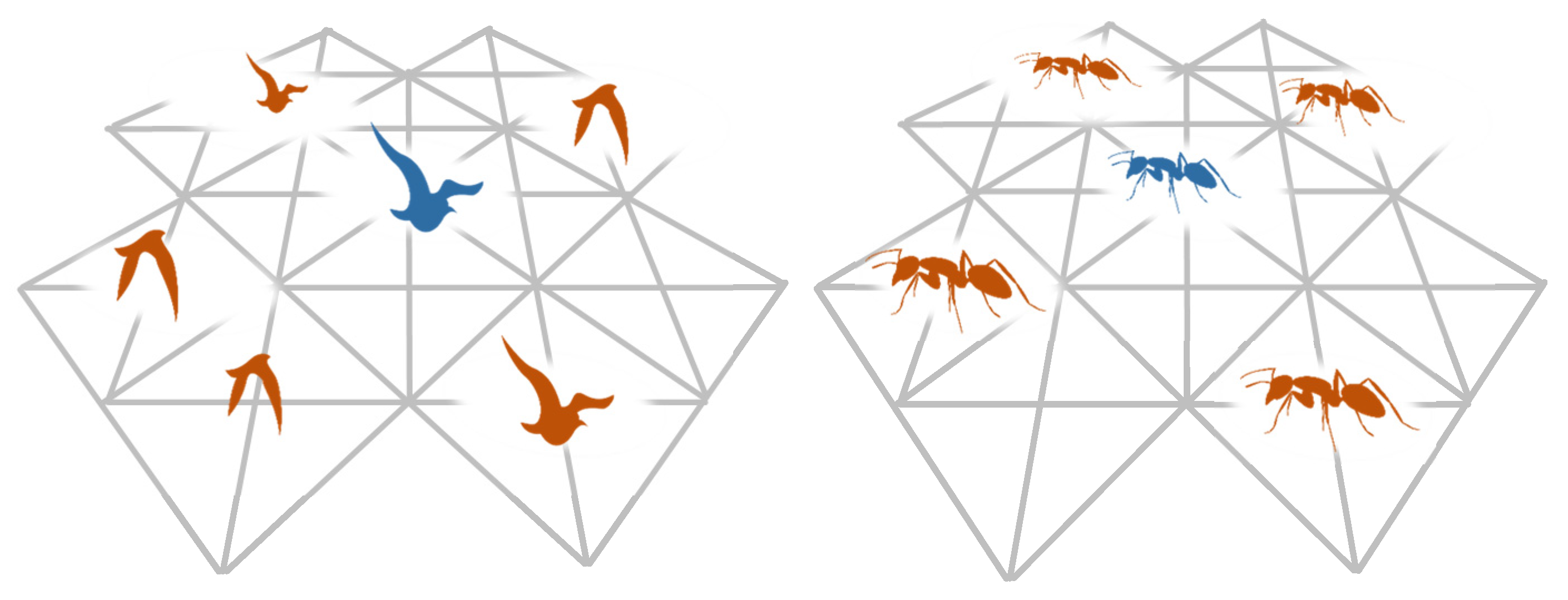
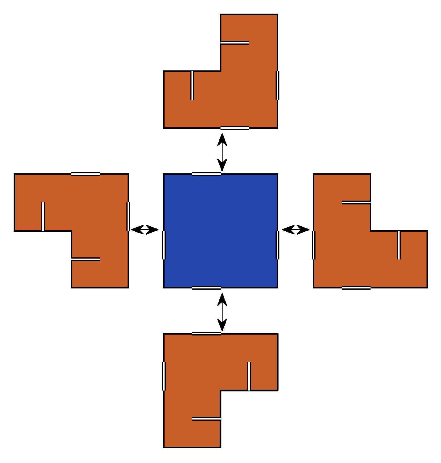
As an alternative to a wired sensors network for smart structures, wireless sensor networks (WSNs) have attracted several researchers [28]. With lower cost, an array of WSNs can effectively be used for monitoring the structural deterioration, as well as controlling vibration during an earthquake, by using artificial neural networks [29,30]. The data that is acquired using WSNs is essentially the same as the traditional counterpart that has been challenged recently due to deployment difficulties, as well as reliability issues during an extreme event. Nowadays it is feasible to mimic the swarm behaviors in nature and share important response data with the adjacent buildings using a wireless sensors network and via cloud-based computing [31]. Keeping this in mind, the idea of swarm-based parallel control (SPC) of such buildings is proposed in this paper. With this approach, the response data from each wireless sensor is transferred to the adjacent buildings to update the responses without physical structural links. Figure 1 illustrates such information flow that is inspired by nature. Using the similar concept for adjacent buildings, the control force can be determined for each building with respect to the other surrounding structures, meaning that using the proposed algorithm, the optimal control forces are first determined based on the response of each building individually, and then, it is modified based on the responses of the other adjacent structures. In this study, the fuzzy inference system (FIS) is used to interpret the data using nonlinear mappings. The nature-inspired information flow among the swarms can be seen in Figure 1, while the information flow between each adjacent building is illustrated in Figure 2.
The goal of this study is to introduce and validate the performance of the proposed algorithm for adjacent buildings, using semi-active MR dampers that are wirelessly controlled by utilizing cloud-based computation. In addition, irregularity and soil–structure interactions are considered in this study. Two pairs of MR dampers are installed on each floor in two directions to suppress coupled translational–torsional motions, which are controlled by implementing the concept of the Internet-of-Things (IoT) and wireless sensor networks (WSNs). Robustness of the proposed method is evaluated and verified using three example cases: a single multi-story building considering the SSI, two adjacent buildings coupled using MR dampers as well as active actuators, and five adjacent buildings controlled using the proposed SPC. The LQR-based active control system is considered to provide benchmark results for comparison purposes only, and the mechanism and advantages of the proposed method over the active tendon controller are not discussed in this study.
2. Analytical Equations of Motion Considering Soil–structure Interaction
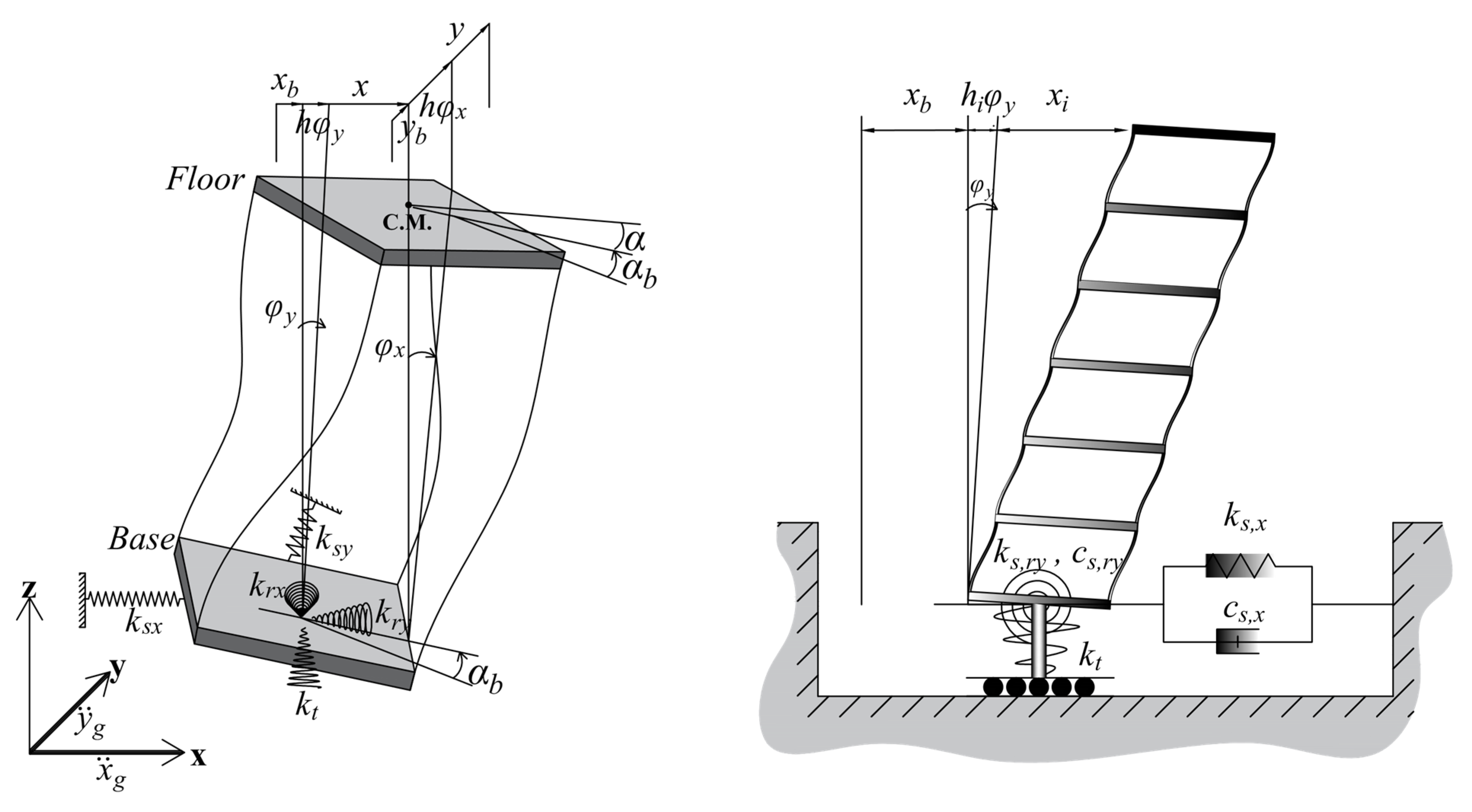
Figure 3 shows a multi-story shear frame building considering the soil–structure interaction simulation. In three-dimensional space, a building can be idealized as a (3 × n Story + 5)-DOF system. This is because each story has three degrees of freedom, plus five degrees of freedom for the base of the structure, swaying motion in the x- and y-directions, rocking about the x and y-axes, and twisting about the z-axis. As shown in Figure 3, pairs of dashpots and springs are defined to consider the SSI effects in the simulations. In this figure, denotes the base displacement, represents the rocking motions about the y-axis, and the relative displacements of stories are shown as . Note that the settlement in the z-direction is not considered, and the twisting motion is not visible from the side view.
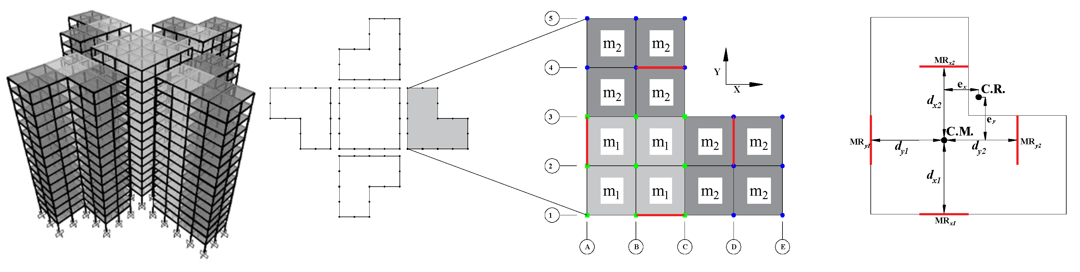
The control devices placement is shown in Figure 4 for the MR devices, and due to the eccentricity with respect to the center of mass, , each device generate a moment to resists the torsional motion. Irregularity in plan and elevation is described by the mass eccentricity with respect to the center of rigidity, and .
The governing equations of motion for a controllable n-story building can be expressed as follows in general,
where , and are the dynamic properties of the building, and , and are the relative (to the ground motion) displacement, velocity and acceleration vectors, respectively. is the coefficient matrix of the input controlling forces, and is the ground motion coefficient vector. The governing equation of motion can be re-written in state-space form as explained in [32]:
where
It should be noted that the above-mentioned equations are in the continuous-time format; however, for the simulation with Matlab software, they are converted to the discrete-time format. A step-by-step procedure for computing the response of the system in the discrete-time domain is presented in the reference book by Cheng et al. [33]. The ground motions coefficients are given in for two directions, and the coefficient of the input controlling forces on each degree of freedom, including rotation, , can be described using the matrix as [32,34]:
where is
Then, the mass and stiffness matrices considering the SSI effects can be assembled as:
where
where is a zero matrix, and is the mass matrix of the story [32].
In the above-mentioned equations, is the mass of the story, the mass moment inertia about each axis in three-dimension is defined as follows for a floor slab with dimensions of , and coordinates of . The center of the mass coordinate is given as .
Similarly, the center of stiffness is located at (, and that of the lateral resisting member with the coordinate has the stiffness of , and in two directions. The column is assumed to have . Thus, the stiffness matrix is assembled as follows [32,34]:
The damping matrix is constructed in the same way as for the stiffness matrix, but the superstructure damping is determined using Rayleigh’s method [35] without SSI. The SSI parameters are determined using the equations given in [25,32,34], which are summarized in Table 1. In this study, two cases with and without SSI effects are investigated. The soft soil is assumed to have the Poisson’s ratio of 0.33, the density of 2400 kg/m2, shear-wave velocity and modulus of 500 m/s and 6 × 10⁸ N/m2, respectively. Details of the SSI models, as well as the methodology, are presented by Nazarimofrad and Zahrai [34].
3. Swarm-Based Parallel Control (SPC)
In this study, three different control alternatives for adjacent buildings are presented and discussed. One most commonly used method is to control each building independently without any information flow (Case-I in this paper). Another approach is to couple two adjacent buildings side-by-side by actuators or additional dampers, such as hydraulic or MR dampers (Case-II in this paper). Both methods are discussed, and the results are compared with the proposed swarm-based parallel control (SPC), which is Case-III in this paper. The SPC algorithm is the FLC for each building, with an additional updating agent that is another FLC to consider the response of the other buildings simultaneously.
For Case-I, the behavior and control of a single building (in the east, Figure 4) are studied considering the soil–structure interaction (SSI) effects, and the performance of the different control algorithms are compared when the behavior of the adjacent structure is neglected. The response reduction ratio is considered as the performance index, and since the active control has a different control mechanism, the ideal condition is considered for this study. The linear quadratic regulator (LQR) algorithm is used for calculating the optimal control forces that can be applied to the structure through pairs of active tendons that can be installed at the same locations as for the MR dampers. Therefore, the advantages of FLC and SPC are not compared to the active control system. The fuzzy logic control (FLC) is used to efficiently control vibrations using semi-active MR dampers, which is illustrated in Figure 5. More details, and the background of LQR and FLC algorithms are available from refs. [32,36,37]. The weight matrices for the LQR method are selected as , and , where is an identity matrix.
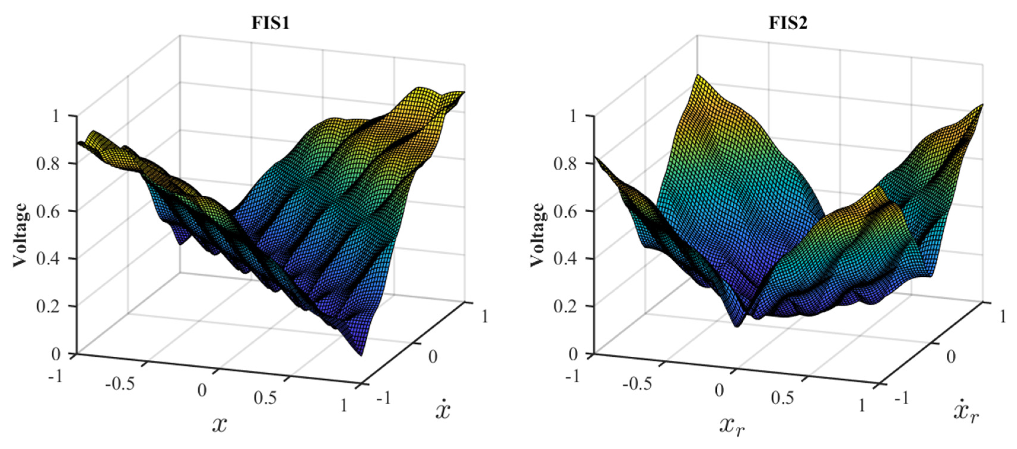
Figure 4 shows five adjacent buildings with different dynamic properties. Instead of coupling buildings (Case-II), response data is shared among the controllers. Thus, an additional control fuzzy logic control layer is considered to avoid pounding, for which the input variables are the relative displacements and the directions. Using this strategy, the optimal required clearance distance can be decreased, which is critical in urban areas, where the cost of space and material is essential. Using this method, the adjacent buildings are not connected physically, and the response data are shared wirelessly. Thus, buildings are independently controlled, and then their relative performances are evaluated using a second fuzzy logic control algorithm. In this paper, the first fuzzy logic control, FIS1, determines the control forces for individual buildings independently, and the second fuzzy logic control, FIS2, determines the control forces based on the relative motions including the torsion in each irregular building. Finally, the optimal MR dampers input voltages are selected by comparing the outputs of FIS1 and FIS2.
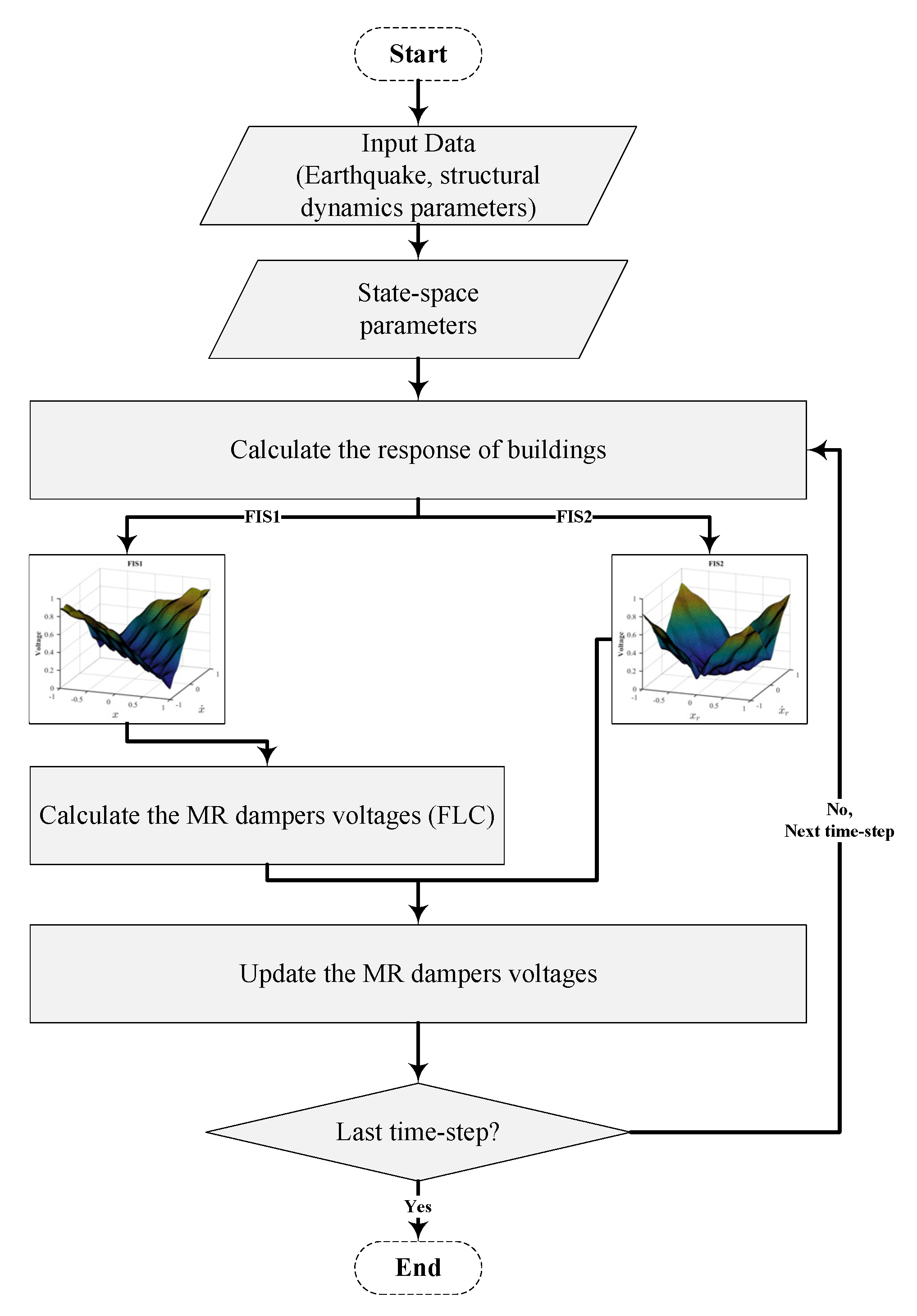
The two surface plots of the outputs are shown in Figure 6 for FIS1 and FIS2 using the Gaussian membership functions for the variables. In Figure 7, the flowchart of the proposed swarm-based control (SPC) is described in summary. The flowchart includes the following steps:
- Step 1.
- Estimating the dynamic properties of the soil as well as the building (e.g., using data-driven-based machine learning models [38]).
- Step 2.
- Assembling the state-space model and equation of motions according to Equations (1)–(12).
- Step 3.
- Calculating the response of each of the adjacent buildings, }, by solving the state-space equations in Step 3.
- Step 4.
- Normalizing the state vector (i.e., measures responses, and calculating the control force using the fuzzy logic control FIS1.
- Step 5.
- Updating the calculated control force in both directions, using the second fuzzy logic-based updating rules, FIS2, based on the relative displacements of two adjacent buildings. In this step, the outputs of FIS1 and FIS2 are compared, and if the FIS2 output is higher than the FIS1 output, the control force is adjusted based on the FIS2 results.
- Step 6.
- Apply the calculated control force, , and continuing until the end of the last time-step.
4. Numerical Studies
4.1. Building Models Discerptions
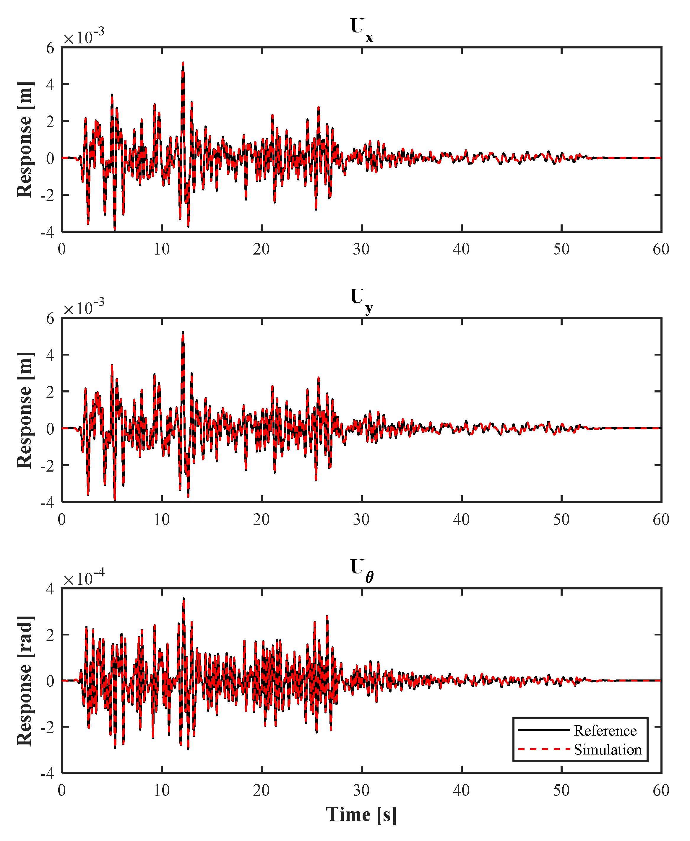
In this paper, four adjacent 15-story irregular steel frame buildings were designed and simulated in MATLAB® (MathWorks, Inc., Nattick, MA, USA), based on the studies carried out by Kaveh et al. [39] and Azimi [32]. The 3D and plan views of the structures, as well as the mass and stiffness distributions, are visually illustrated in Figure 4. Two groups of columns, with the same stiffness in both directions, are connected rigidly to the floor diaphragm frames, Kn/m. Each floor consists of 5 × 5 m2 slabs that carry loads of (kN/m2) to simulate the eccentricity. Each story has a height of 3.0 m, except the first story, with a 3.2 m height. The four dampers of each floor are placed within the frames shown with red bold lines. To ensure the accuracy of the simulation results, the building model simulation is verified, based on the study by Nazarimofrad et al. [34]. Figure 8 shows the top floor level response of the 10-story building model under the same ground motion, which indicates that the simulation results in this study are valid.
4.2. Magneto-Rheological (MR) Damper
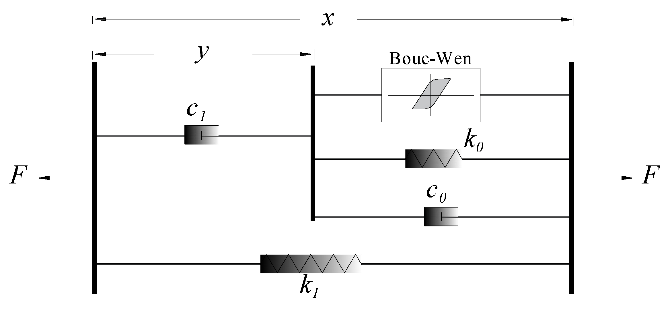
The phenomenological model for the MR damper was first proposed by Spencer et al. [40], based on the Bouc–Wen model in 1997. Nowadays, the MR damper is one of the most reliable devices for seismic vibration control applications. The advantage of the MR damper is its role in the case of power loss, which provides minimum damping based on its shaft displacement and velocity. Using a semi-active control algorithm, the control command is the input voltage of the MR damper. The modified model of MR damper is given in Figure 9. The notation in Figure 9 and Equations (13)–(16) denotes the relative displacement of the two ends of each MR damper.
More details are available in the literature regarding the history of the development of the analytical model of MR dampers. According to Spencer et al. [40], the nonlinear behavior of an MR damper can be described as follows
where F is the nonlinear force of the MR damper (included in ), is the accumulator stiffness, and z is the evolutionary variable of the hysteretic, defined as:
where γ, β and A are the shape parameters, and the α, c0 and c1 can be obtained using the following linear functions of the efficient voltage, u.
The parameters of the MR damper are given in Table 2.
4.3. Earthquake Loads
5. Results and Discussion
Irregularity in high-rise buildings is an important factor in evaluating the seismic responses, due to the higher modes effects under bidirectional seismic loads [32]. Under the bidirectional earthquake loads, it is clear that higher modes of an irregular structure will have a significant impact on the results, particularly considering the soil–structure interaction effect. In the following sections, the structural responses of the buildings are discussed in detail for the three chases.
5.1. Control of Single Building Considering Soil–structure Interaction (Case I)
5.1.1. Peak Responses
The peak responses of the Case-I building under the seven selected earthquake records are given in Table 4, which includes the maximum top floor transversal and rotational displacements, and also the accelerations in two directions. The optimal active control responses are obtained using a full-state LQR controller. For the passive-min and passive-max cases, also known as passive-off and passive-on, the input voltage for each MR damper is constant and equal to 0 and 9 volts, respectively. In the case of power loss, and under the seven earthquakes given in the table, the passive-min case offers 13%, 8%, 10%, 3%, 13%, 8% and 14% reduction in transversal displacements, when the building is on soft soil. The response reduction percentages are approximately 30% smaller for the same building on the rock base.
The passive-max case, however, provides 40–50% more reduced compared with the passive-min control. Using the FLC offers even more maximum response reduction, which is about 60%, 40%, 55%, 38%, 47%, 38% and 52% for the building on soft soil under the seven selected earthquakes, respectively. For the building on a rock base, the FLC is 10% less efficient, however. Comparing the maximum responses for the active control scenario, where the controlling tendons are assumed to deliver the real-time control forces with minimum errors, reveals that this method does not provide the same performance under the Chi-Chi earthquake for the same building on rock and soft soil bases. Despite the 50–66% displacement response reduction for the building on the rock base, active control causes the displacement responses to be increased by 32% and 154% in two directions. In general, it can be seen that the peak responses are smaller for the buildings on the soft soil, except for the active control under the Chi-Chi earthquake. Therefore, the FLC offers reliable performance from this point of view, and it is used for the Parallel control of adjacent buildings.
5.1.2. Time-History Responses
The time-history responses provide a tool to understand the performance of any techniques during a seismic event [42]. Figure 11 shows the top floor displacement time-history in the x-, y-, and θ- directions for the Case-I building considering SSI under the Chi-Chi earthquake. It is clear that the designed active control for a building on a rock base does not necessarily have similar performance for the same building, but on a soft soil base. This different behavior shows the sensitivity of the active control system, as well as the reliability of the FLC method. For all the seven earthquakes, the FLC provided a better performance with and without considering SSI. Another important fact, evident from the peak responses table and the time-history curves, is that for those buildings on a soft soil base, the peak responses are smaller. By implementing a properly designed FLC, the overall response can be reduced by 40% and 50% for near- and far-field earthquakes, respectively [32].
5.1.3. Inter-Story Drift and Lateral Displacement Profiles
The inter-story drift profiles are typically used as a measure for the optimal placement of control devices, as well as estimating the potential damage locations. Smaller inter-story drifts, on the other hand, indicate that linear control algorithms can be satisfactory. Furthermore, P-Δ effects are reduced by decreasing the inter-story in the lower levels of a multi-story building. Smaller inter-story values for top floors makes it reasonable to use twin tuned mass dampers (TTMDs) instead of semi-active dampers, since the performance of semi-active devices is directly related to the relative displacement and velocity [37]. Figure 12 and Figure 13 show the maximum inter-story drift profiles for the Case-I building in x-direction, under the bidirectional earthquakes loads. For this specific example, the active control using LQR algorithms shows a better performance in most of the cases.
The Chi-Chi earthquake is a good example to explain two different behaviors for the same controller, which highlights the importance of the additional five degrees of freedom (DOF) from the SSI. Similar differences can be seen under the El-Centro earthquake. From the displacement profiles, it is evident that in the case of power loss, Passive-Min, MR dampers still contribute to the response reduction by providing a small amount of damping [36]. The absolute displacement profiles provide useful tools to better understand the vibration control of adjacent buildings that are discussed in Case-II and Case-III buildings.
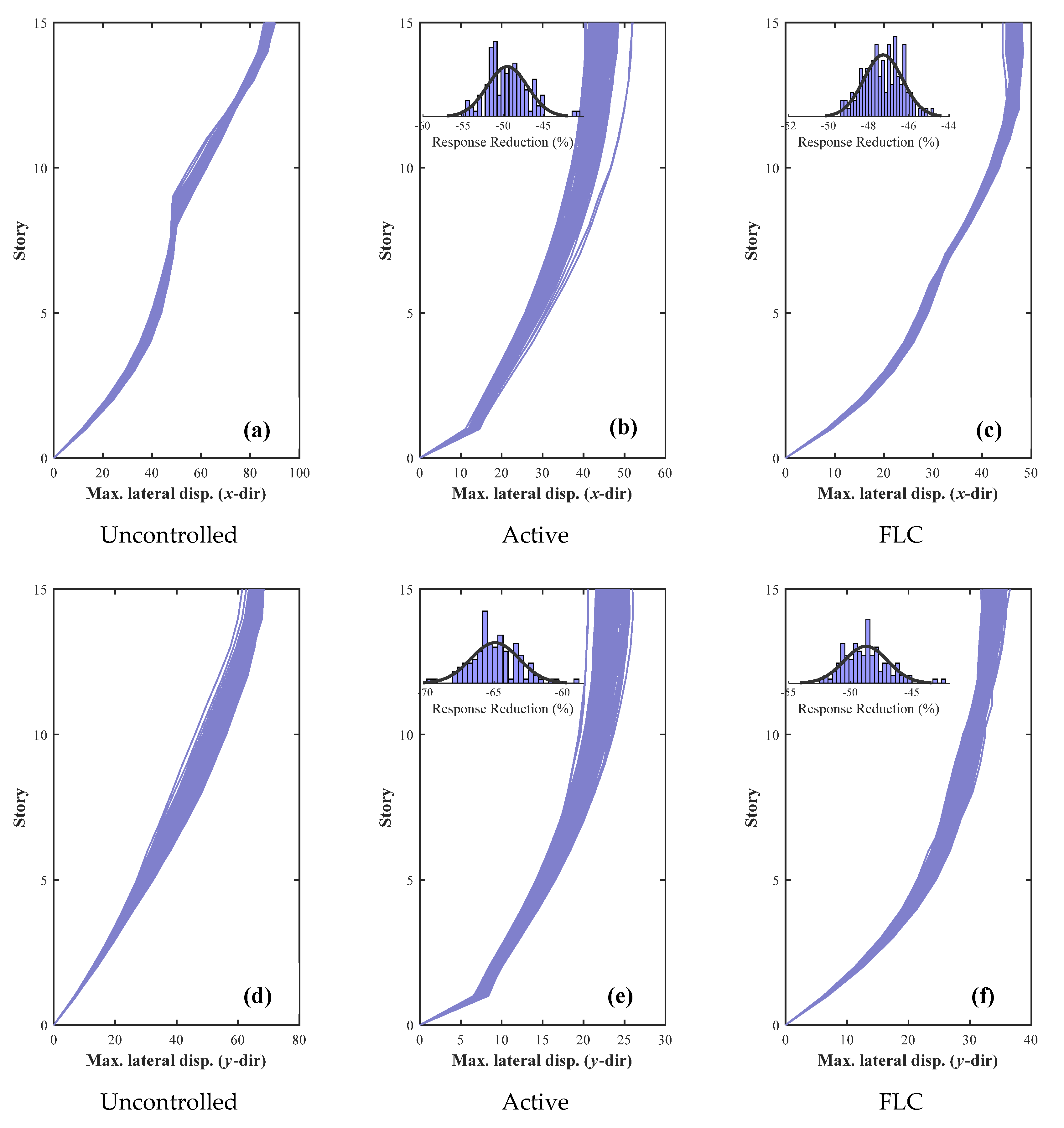
Estimating the soil properties, as well as the dynamic characteristics of buildings, are not always accurate. To study the sensitivity of the structural responses, as well as the performance of the controller under uncertainties, a total of 120 random building models were generated, using 14 random variables for soil and structure models. The distribution of each random variable is assumed to be a Normal Gaussian with a coefficient of variation of 5%. In addition, 1% noise added to all the measurements. The results are provided in Figure 14, which includes the maximum lateral response profiles from each analysis, as well as the response reduction distribution for the top floor level in both directions. According to the results, it can be said that the FLC is less sensitive to the soil type based on the range of the histogram plots for the response reduction percentages for each case, however, the active control is highly sensitive to the estimated dynamic properties of the system. Therefore, fuzzy logic-based controllers are suitable for the proposed approach in this study. It is worth it to mention that the response variation in y-direction for the FLC controlled is higher than the x-direction, however, both have similar distribution as for the uncontrolled cases.
5.2. Advantages of WSNs in Case of Structural Damage or Control Failure
One of the main drawbacks of the traditional wired sensor networks, is that they are not always reliable in case of fire, or due to the failure of signal lines at lower floor levels under large deformations. On the other hand, IoT and cloud-based computation, along with wireless sensor networks, make each device independently controllable and more reliable. The effect of the failure in the signal line in the traditional wired and wireless network are compared in Figure 15. In the wired sensor network, expecting that the main controlling computer remains safe and secured during an earthquake, the signal line is assumed to be broken at either the 4th or 6th floor, which would put the upper floors controlling devices in passive-min mode. However, using the IoT concept with a wireless sensors network, only the specified floor dampers are removed from the control algorithm. The overall structural responses of the building on the top floor in x-, y-, and θ-directions using the FLC indicate the superior performance of a wireless sensor network as part of the IoT. Comparing the responses also reveals that placing MR dampers at the first lower floors offers more resistance and damping during an earthquake, which is reasonable referring to the inter-story drift profiles.
5.3. Pounding Hazard Mitigation by Coupling (Case-II)
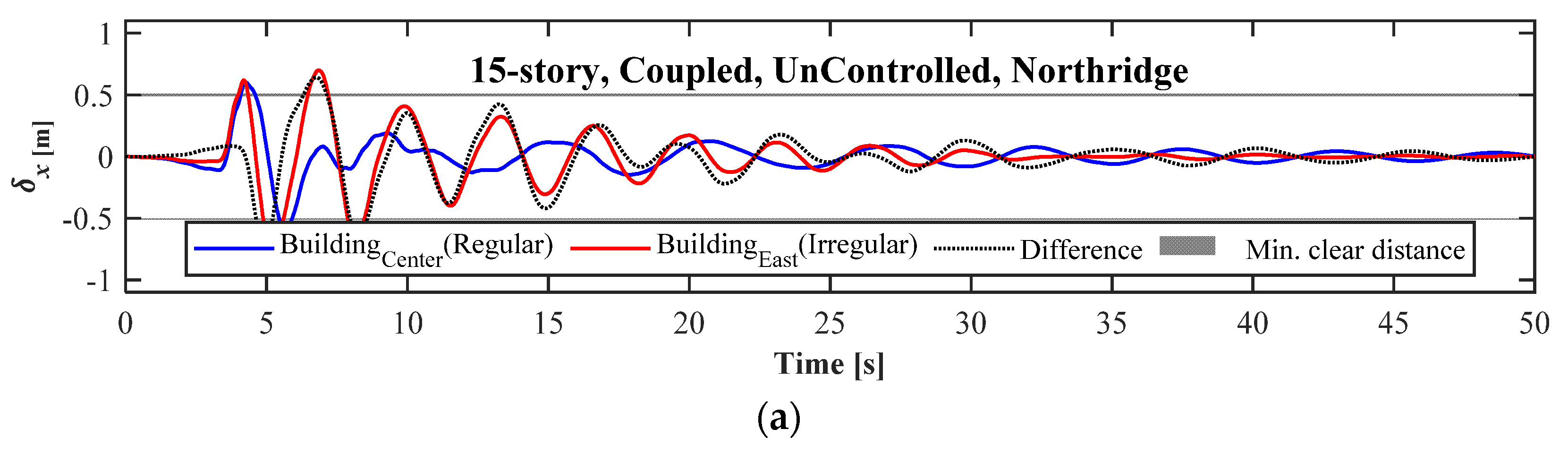
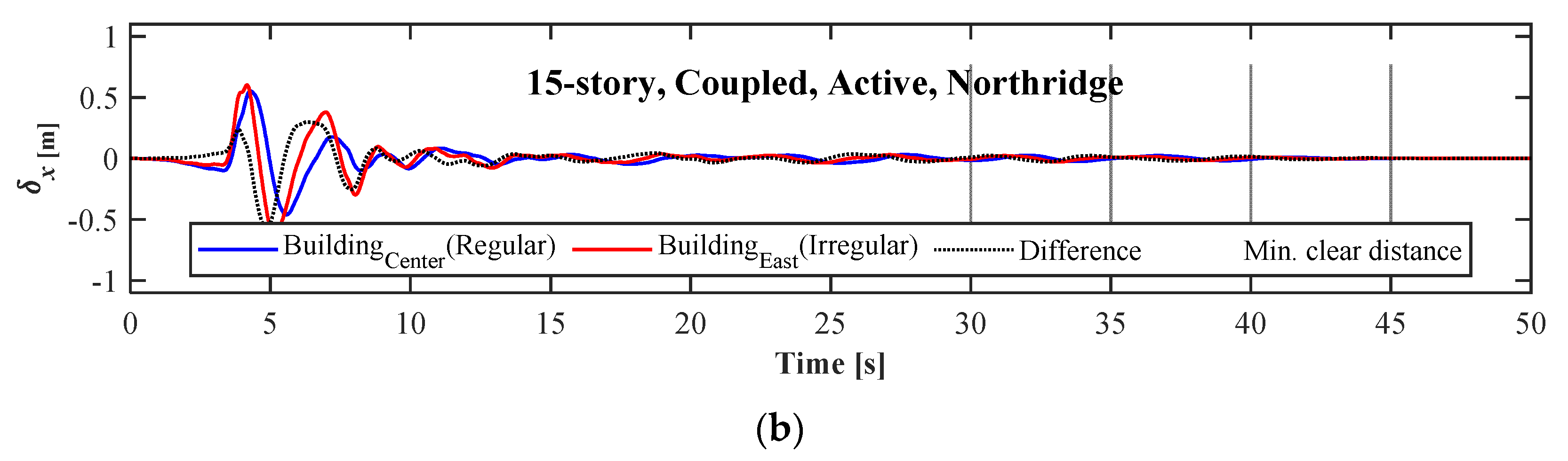
Design of a vibration control algorithm, when at least one of the two adjacent buildings is irregular, is a challenging task that needs knowledge and experience. To reveal one of the main challenges of designing an active control using active tendons to couple two buildings, which includes the optimal selection of the weights, the vibration responses of the two adjacent buildings, in the east (irregular) and the center (regular), are given in Figure 16. As it is clear from the figure, under the Northridge earthquake loads, the vibration of both buildings decreases significantly, as well as a considerable decrease in the minimum clear distance between the two buildings, considering the irregularity. These results are obtained when the parameters of the LQR algorithm is selected by an optimization technique. With this technique, the irregular building in the east passes a portion of lateral loads to the regular building to reduce the overall response of both, which can be seen from the results that indicate a minimum reduction in the peak displacement in the directions to the adjacent structure.
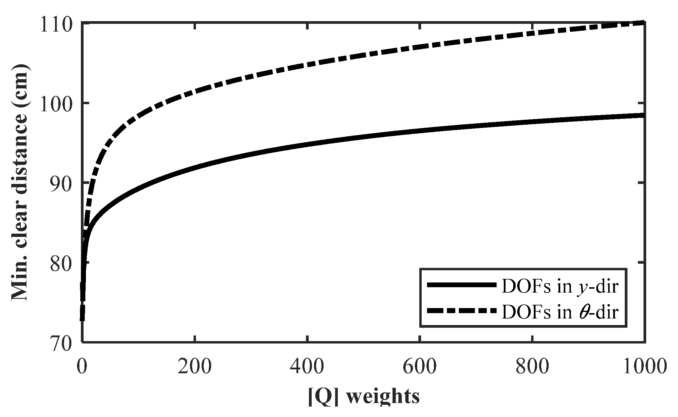
Figure 17, on the other hand, clearly shows that using an LQR-based active control for two coupled regular-irregular buildings are sensitive to the initial assessment of the dynamic properties of the system, as well as the selection of the LQR parameters. In this figure, two curves illustrate how the minimum clear distance between the two buildings increases as the weight coefficient on the response of specific DOFs in a direction changes, without updating the response weights in the other two directions. In this example, the response weight corresponding to the DOFs in the x-direction, as well as another direction (y or θ), is given a unit coefficient, while the response weights of the DOFs in the third direction changes. Comparing the two curves shows that restricting the rotational vibration would result in more increase in the minimum clear distance required to avoid pounding, compared to the response in the perpendicular direction. Therefore, an optimized solution needs to be achieved using the evolutionary algorithms, if active control is an option for controlling coupled buildings with irregularity and SSI effects. Another major concern with coupling two buildings (Case-II) is that larger relative displacements may not be suitable for the application of MR dampers that are sensitive to shaft displacement and velocity. Due to such reasons, the application of MR dampers, as the connectors of two coupled buildings, is not recommended for this specific case study.
5.4. Advantages of SPC over Traditional FLC (Case-III)
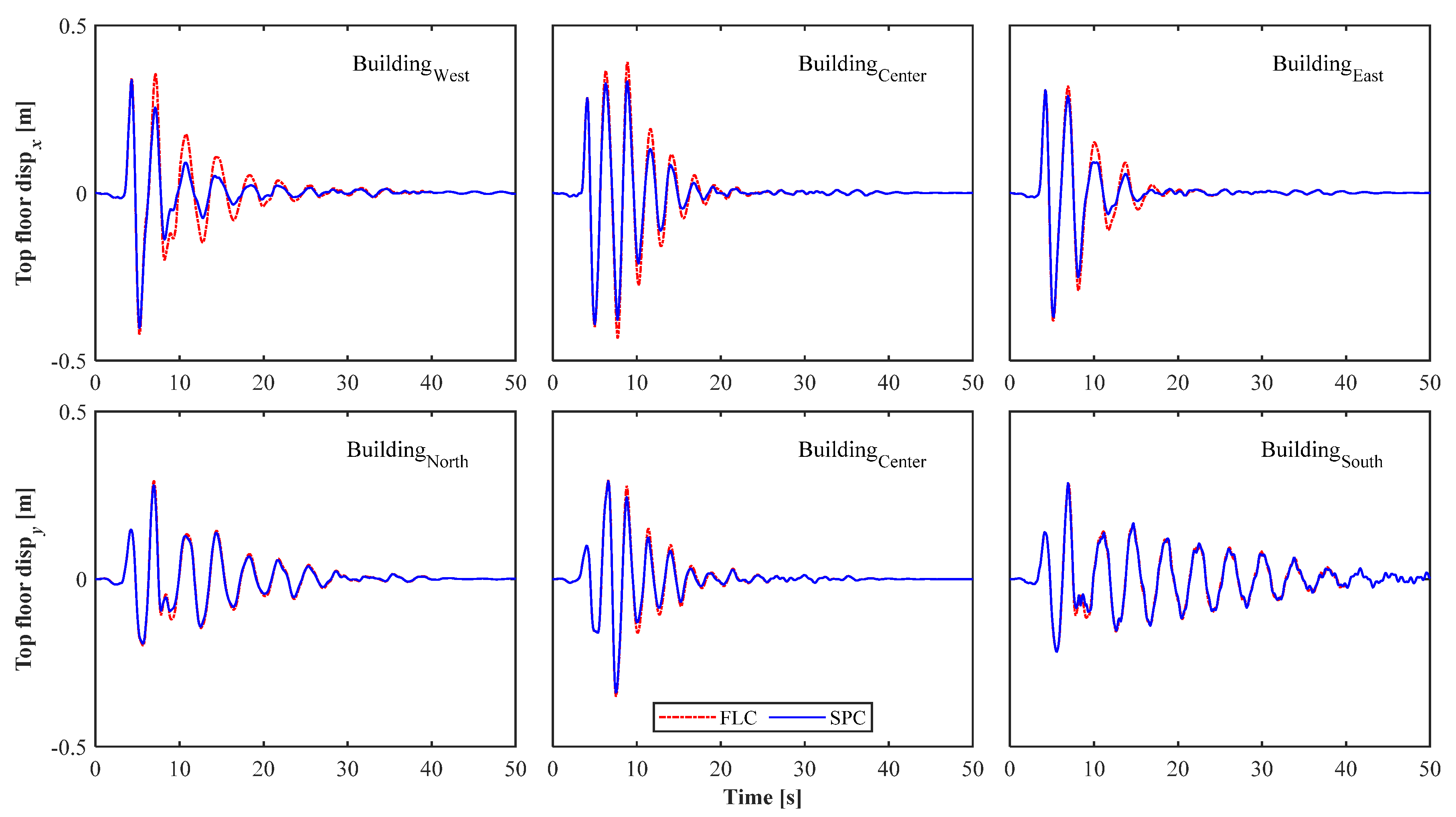
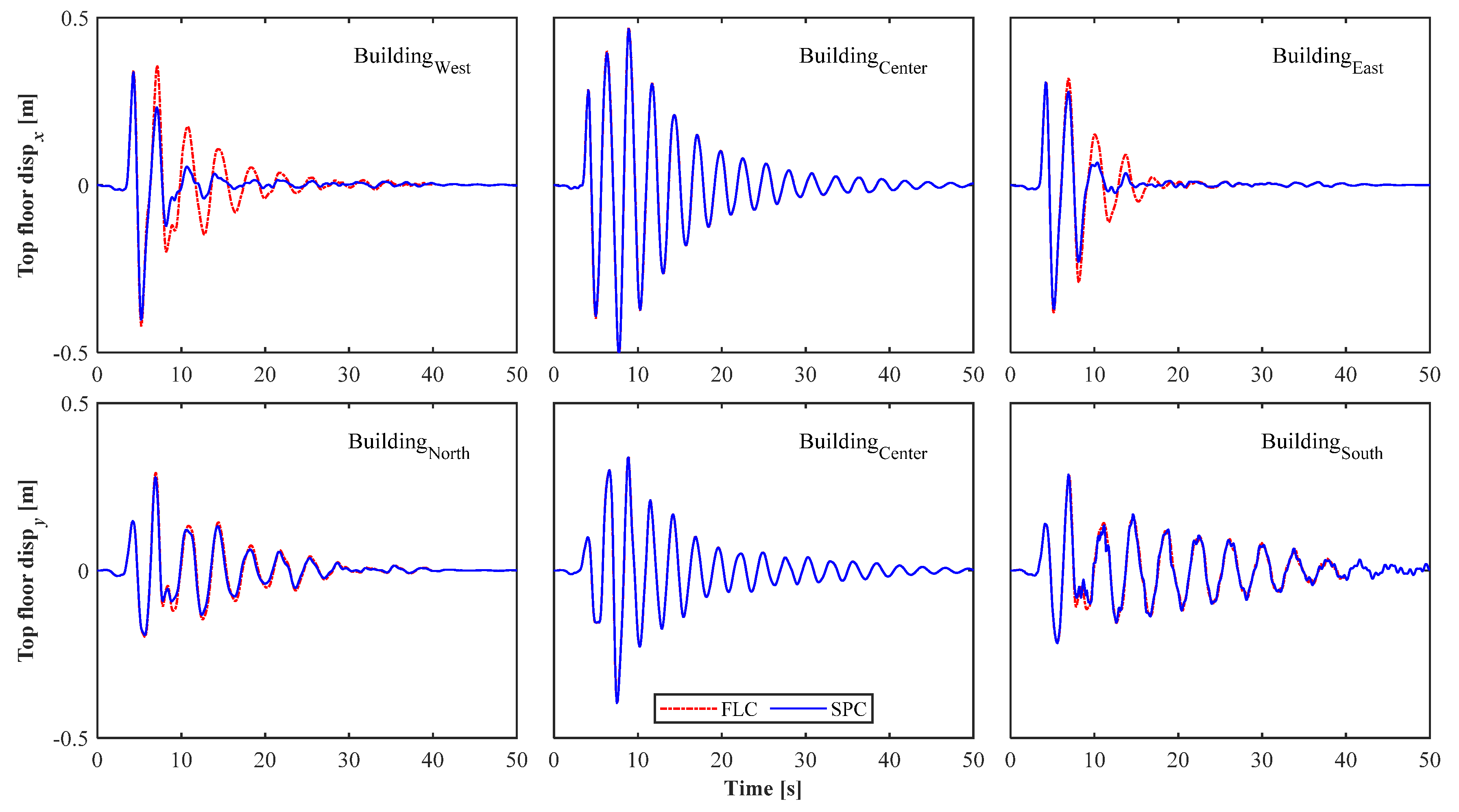
The proposed SPC includes two FLCs in the main control flowchart, however, there are some advantages for the SPC, which a typical FLC may not be able to consider. Figure 18 shows the top floor displacement response of the five adjacent buildings under the bidirectional loads of the Northridge earthquake. The first row of the figure corresponds to the responses in the x-direction, which includes the buildings in the west, center and east (information flow in west-east direction). Similarly, the second row represents the responses in the y-direction, which shows the information flow among the buildings in the north, center and south. According to the information flow rule among the adjacent buildings for the proposed SPC, it is obvious that for regular adjacent buildings, the control algorithms are independents in two directions; however, for the current case (Case-III), controlling the vibrations in one direction influences the response in the other direction through torsional vibrations in the top floors. Since the stronger component of the Northridge earthquake is applied in the x-direction, the differences in the responses are obvious in this direction.
To investigate the performance of the proposed SPC algorithm in the case of damage, the buildings are excited under the Northridge earthquake. Based on the obtained lateral drift profiles, it is assumed that the first five floors of the building in the center lose the lateral stiffness in a way that the maximum and minimum damages in a range of 50%~25%, respectively, occur in the first and fifth floor. Besides, the control system of the building is shut down at the 5th second after the activation, when the drifts reach approximately maximum values. Therefore, the minimum damping capacities of the dampers are used for the rest of the excitation. Under this situation, it is expected that using the proposed SPC algorithm, the adjacent buildings will change their behavior to avoid pounding hazards. Figure 19 shows the response time-histories for the buildings with and without consideration of damage in the central building. It is clear that the top floor displacements of the building in the center are increased in both directions; however, the adjacent buildings behave differently, but with a reduction in the responses.
6. Summary and Conclusions
The majority of the studies in seismic vibration control of three-dimensional tall buildings have not considered the irregularity and soil–structure interaction effects on the vibration response. In this paper, a novel bio-inspired seismic vibration control algorithm, called swarm-based parallel control (SPC), is proposed to use the advantages of fuzzy logic-based rules to consider the response of the individual adjacent building in determining the control forces for the group of buildings during extreme events, such as earthquake or wind loads. The main merits of the proposed SPC system can be summarized as:
- Despite the other control approaches, such as using coupling devices, the need for the structural links to couple the two adjacent buildings, as well as the complexity, can be eliminated.
- Each building can sense and consider the responses of the adjacent building in determining the optimal control force of semi-active devices; therefore, in the case of damage in a building, the other adjacent buildings update the control forces, accordingly.
- The proposed SPC can be modified for individual buildings according to the deployed control strategy and devices.
To address the above-mentioned advantages of the proposed controller, numerical simulations are carried out under the seismic loads of seven historic earthquakes. Vibration responses of an irregular 15-story building are studied considering the soil–structure interaction (SSI) effect, as well as the effectiveness of different control methods (Case-I). A sensitivity analysis is also considered to study the performance of each control approach, considering uncertainties in estimating the soil and structural properties. In addition, the idea of coupling two adjacent regular-irregular buildings is discussed using an ideal active control, regardless of the control device type, and the limitations are highlighted (Case-II). It should be noted that for the active control system, the results are obtained based on the LQR algorithm to have a benchmark result for comparison, and the ideal conditions are assumed for either method. Finally, five adjacent buildings with different dynamic properties and no structural connections, considering the SSI effects, are modeled to verify the performance of the proposed SPC algorithm (Case-II).
The results prove that the proposed method has the potential to be paid attention in future developments as part of the bigger concept of the Internet-of-Things (IoT) and smart structures.
Author Contributions
Conceptualization, M.A.; methodology, M.A.; software, M.A. and A.M.Y; validation, M.A.; formal analysis, M.A.; investigation, M.A. and A.M.Y.; resources, M.A.; data curation, M.A. and A.M.Y.; writing—original draft preparation, M.A.; writing—review and editing, M.A. and A.M.Y.; visualization, M.A.; supervision, M.A. All authors have read and agreed to the published version of the manuscript.
Funding
This project did not receive funding.
Acknowledgments
This study was initiated in 2018 based on Azimi [32], and the authors acknowledge and highly appreciate Zhibin Lin’s academic support in the early stages of this study, from North Dakota State University.
Conflicts of Interest
The authors declare no conflict of interest.
References
- Mosleh, A.; Rodrigues, H.; Varum, H.; Costa, A.; Arêde, A. Seismic behavior of RC building structures designed according to current codes. Structures 2016, 7, 1–13. [Google Scholar] [CrossRef]
- Azimi, M. Stiffeners Effect on Seismic Performance of I-Beam to Double-I Built-up Column Connection. Master’s Thesis, Iran University of Science and Technology, Tehran, Iran, November 2011. [Google Scholar]
- Amiri, G.G.; Azimi, M.; Darvishan, E. Retrofitting I-beam to double-I built-up column connections using through plates and T-stiffeners. Sci. Iran. 2013, 20, 1695–1707. [Google Scholar]
- Lin, J.L.; Tsai, K.C. Seismic analysis of two-way asymmetric building systems under bi-directional seismic ground motions. Earthq. Eng. Struct. Dyn. 2008, 37, 305–328. [Google Scholar] [CrossRef]
- Mashayekhi, M.; Santini-Bell, E. Three-dimensional multiscale finite element models for in-service performance assessment of bridges. Comput. Aided Civ. Inf. 2019, 34, 385–401. [Google Scholar] [CrossRef]
- Mashayekhizadeh, M. Fatigue Assessment of Complex Structural Components of Steel Bridges Integrating Finite Element Models and Field-Collected Data. Ph.D. Thesis, University of New Hampshire, Durham, NH, USA, 2018. [Google Scholar]
- Mohammadi, R.K.; Nasri, A.; Ghaffary, A. TADAS dampers in very large deformations. Int. J. Steel Struct. 2017, 17, 515–524. [Google Scholar] [CrossRef]
- Ghaffary, A.; Karami Mohammadi, R. Framework for virtual hybrid simulation of TADAS frames using opensees and abaqus. J. Vib. Control. 2018, 24, 2165–2179. [Google Scholar] [CrossRef]
- Amini, F.; Samani, M.Z. A wavelet-based adaptive pole assignment method for structural control. Comput. Aided Civ. Inf. 2014, 29, 464–477. [Google Scholar] [CrossRef]
- Uz, M.E.; Hadi, M.N.S. Optimal design of semi active control for adjacent buildings connected by MR damper based on integrated fuzzy logic and multi-objective genetic algorithm. Eng. Struct. 2014, 69, 135–148. [Google Scholar] [CrossRef] [Green Version]
- Abdeddaim, M.; Ounis, A.; Djedoui, N.; Shrimali, M.K. Pounding hazard mitigation between adjacent planar buildings using coupling strategy. J. Civ. Struct. Health Monit. 2016, 6, 603–617. [Google Scholar] [CrossRef]
- Chandiramani, N.K.; Motra, G.B. Lateral-torsional response control of MR damper connected buildings. In Proceedings of the ASME 2013 International Mechanical Engineering Congress and Exposition, San Diego, CA, USA, 15–21 November 2013. [Google Scholar]
- Bozorgvar, M.; Zahrai, S.M. Semi-active Seismic Control of Buildings Using MR Damper and Adaptive Neural-fuzzy Intelligent Controller Optimized with Genetic Algorithm. J. Vib. Control 2019, 25, 273–285. [Google Scholar] [CrossRef]
- Kaveh, A.; Dadras Eslamlou, A. An efficient two-stage method for optimal sensor placement using graph-theoretical partitioning and evolutionary algorithms. Struct. Control Health 2019, 26, e2325. [Google Scholar] [CrossRef]
- Kaveh, A.; Dadras, A. Structural damage identification using an enhanced thermal exchange optimization algorithm. Eng. Optimiz. 2018, 50, 430–451. [Google Scholar] [CrossRef]
- Cimellaro, G.P.; Lopez-Garcia, D. Algorithm for design of controlled motion of adjacent structures. Struct. Control Health 2011, 18, 140–148. [Google Scholar] [CrossRef]
- Anajafi, H.; Poursadr, K.; Roohi, M.; Santini-Bell, E. Effectiveness of Seismic Isolation for Long-period Structures Subject to Far-field and Near-field Excitations. Front. Built Environ. 2020, 6, 24. [Google Scholar]
- Roohi, M.; Hernandez, E.M.; Rosowsky, D. Nonlinear Seismic Response Reconstruction and Performance Assessment of Instrumented Wood-frame Buildings—Validation using NEESWood Capstone Full-Scale Tests. Struct. Control Health 2019, 26, e2373. [Google Scholar] [CrossRef]
- Hernandez, E.; Roohi, M.; Rosowsky, D. Estimation of element-by-element demand-to-capacity ratios in instrumented SMRF buildings using measured seismic response. Earthq. Eng. Struct. Dyn 2018, 47, 2561–2578. [Google Scholar]
- Cruz, E.F.; Cominetti, S. Three-dimensional buildings subjected to bi-directional earthquakes. Validity of analysis considering uni-directional earthquakes. In Proceedings of the 12th World Conference on Earthquake Engineering, Auckland, New Zeland, 30 January–4 February 2000. [Google Scholar]
- Heo, J.S.; Lee, S.K.; Park, E.; Lee, S.H.; Min, K.W.; Kim, H.; Jo, J.; Cho, B.H. Performance test of a tuned liquid mass damper for reducing bidirectional responses of building structures. Struct. Des. Tall Spec. 2009, 18, 789–805. [Google Scholar] [CrossRef]
- Yanik, A.; Aldemir, U.; Bakioglu, M. A new active control performance index for vibration control of three-dimensional structures. Eng. Struct. 2014, 62, 53–64. [Google Scholar] [CrossRef]
- Nigdeli, S.M.; Boduroğlu, M.H. Active Tendon Control of Torsionally Irregular Structures under Near-Fault Ground Motion Excitation. Comput. Aided Civ. Inf. 2013, 28, 718–736. [Google Scholar] [CrossRef]
- Wu, W.H.; Wang, J.F.; Lin, C.C. Systematic assessment of irregular building–soil interaction using efficient modal analysis. Earthq. Eng. Struct. Dyn. 2001, 30, 573–594. [Google Scholar] [CrossRef]
- Wolf, J.P. Soil-structure-interaction analysis in time domain. Nucl. Eng. Des. 1989, 111, 381–393. [Google Scholar] [CrossRef]
- Lin, C.-C.; Chang, C.-C.; Wang, J.-F. Active control of irregular buildings considering soil–structure interaction effects. Soil. Dyn. Earthq. Eng. 2010, 30, 98–109. [Google Scholar] [CrossRef] [Green Version]
- Farshidianfar, A.; Soheili, S. Ant colony optimization of tuned mass dampers for earthquake oscillations of high-rise structures including soil–structure interaction. Soil. Dyn. Earthq. Eng. 2013, 51, 14–22. [Google Scholar] [CrossRef]
- Alavi, A.H.; Hasni, H.; Lajnef, N.; Chatti, K.; Faridazar, F. An intelligent structural damage detection approach based on self-powered wireless sensor data. Automat. Constr. 2016, 62, 24–44. [Google Scholar] [CrossRef]
- Ashtiani, R.S.; Little, D.N.; Rashidi, M. Neural network based model for estimation of the level of anisotropy of unbound aggregate systems. Transp. Geotech. 2018, 15, 4–12. [Google Scholar] [CrossRef]
- Roohi, M.; Hernandez, E.M. Performance-based Post-earthquake Decision-making for Instrumented Buildings. arXiv 2020, arXiv:2002.11702. [Google Scholar]
- Gerist, S.; Maheri, M.R. Multi-stage approach for structural damage detection problem using basis pursuit and particle swarm optimization. J. Sound. Vib. 2016, 384, 210–226. [Google Scholar] [CrossRef]
- Azimi, M. Design of Structural Vibration Control Using Smart Materials and Devices for Earthquake-Resistant and Resilient Buildings. Master’s Thesis, North Dakota State University, Fargo, ND, USA, 2017. [Google Scholar]
- Cheng, F.Y.; Jiang, H.; Lou, K. Smart Structures: Innovative Systems for Seismic Response Control; CRC Press: Boca Raton, FL, USA, 2008. [Google Scholar]
- Nazarimofrad, E.; Zahrai, S.M. Seismic control of irregular multistory buildings using active tendons considering soil–structure interaction effect. Soil. Dyn. Earthq. Eng. 2016, 89, 100–115. [Google Scholar] [CrossRef]
- Chopra, A.K. Dynamics of Structures: Theory and Applications to Earthquake Engineering; Prentice Hall: Upper Saddle River State, NJ, USA, 2011. [Google Scholar]
- Azimi, M.; Rasoulnia, A.; Lin, Z.; Pan, H. Improved semi-active control algorithm for hydraulic damper-based braced buildings. Struct. Control Health 2017, 24, e1991. [Google Scholar] [CrossRef]
- Azimi, M.; Pan, H.; Abdeddaim, M.; Lin, Z. Optimal Design of Active Tuned Mass Dampers for Mitigating Translational–Torsional Motion of Irregular Buildings. In Proceedings of the 7th International Conference on Experimental Vibration Analysis for Civil Engineering Structures, San Diego, CA, USA, 12–14 July 2017; pp. 586–596. [Google Scholar]
- Azimi, M.; Pekcan, G. Structural Health Monitoring Using Extremely Compressed Data through Deep Learning. Comput. Aided Civ. Inf. 2019. [Google Scholar] [CrossRef]
- Kaveh, A.; Bakhshpoori, T.; Azimi, M. Seismic optimal design of 3D steel frames using cuckoo search algorithm. Struct. Des. Tall Spec. 2015, 24, 210–227. [Google Scholar] [CrossRef]
- Dyke, S.J.; Spencer, B.F.; Sain, M.K.; Carlson, J.D. Phenomenological model of a magnetorheological damper. J. Eng. Mech. ASCE 1997, 123, 230–238. [Google Scholar]
- Nugroho, P.W.; Li, W.; Du, H.; Alici, G.; Yang, J. An Adaptive Neuro Fuzzy Hybrid Control Strategy for a Semiactive Suspension with Magneto Rheological Damper. Adv. Mech. Eng. 2014, 6, 487312. [Google Scholar] [CrossRef]
- Hu, Y.; Liu, L.; Rahimi, S. Seismic vibration control of 3D steel frames with irregular plans using eccentrically placed MR dampers. Sustainability 2017, 9, 1255. [Google Scholar] [CrossRef] [Green Version]
Figure 1.
Examples of swarm intelligence in nature and information flow among individuals.

Figure 2.
The information flow between five adjacent buildings for the proposed swarm-based parallel control (SPC) (plan view).
Figure 2.
The information flow between five adjacent buildings for the proposed swarm-based parallel control (SPC) (plan view).

Figure 3.
The idealized model of the soil–structure system.

Figure 4.
The configuration of the adjacent buildings used in this study.

Figure 5.
The fuzzy logic control block diagram (Type: Mamdani).

Figure 6.
The surface plot of the FIS1 and FIS2, which are used in the SPC algorithm.

Figure 7.
The flowchart of the proposed swarm-based parallel control (SPC).

Figure 8.
Verification of the simulation for an uncontrolled 10-story building based on Nazarimofrad and Zahrai [34].
Figure 8.
Verification of the simulation for an uncontrolled 10-story building based on Nazarimofrad and Zahrai [34].

Figure 9.
Modified Bouc–Wen model of the magnetorheological (MR) damper (replotted based on Nugroho et al. [41]).
Figure 9.
Modified Bouc–Wen model of the magnetorheological (MR) damper (replotted based on Nugroho et al. [41]).

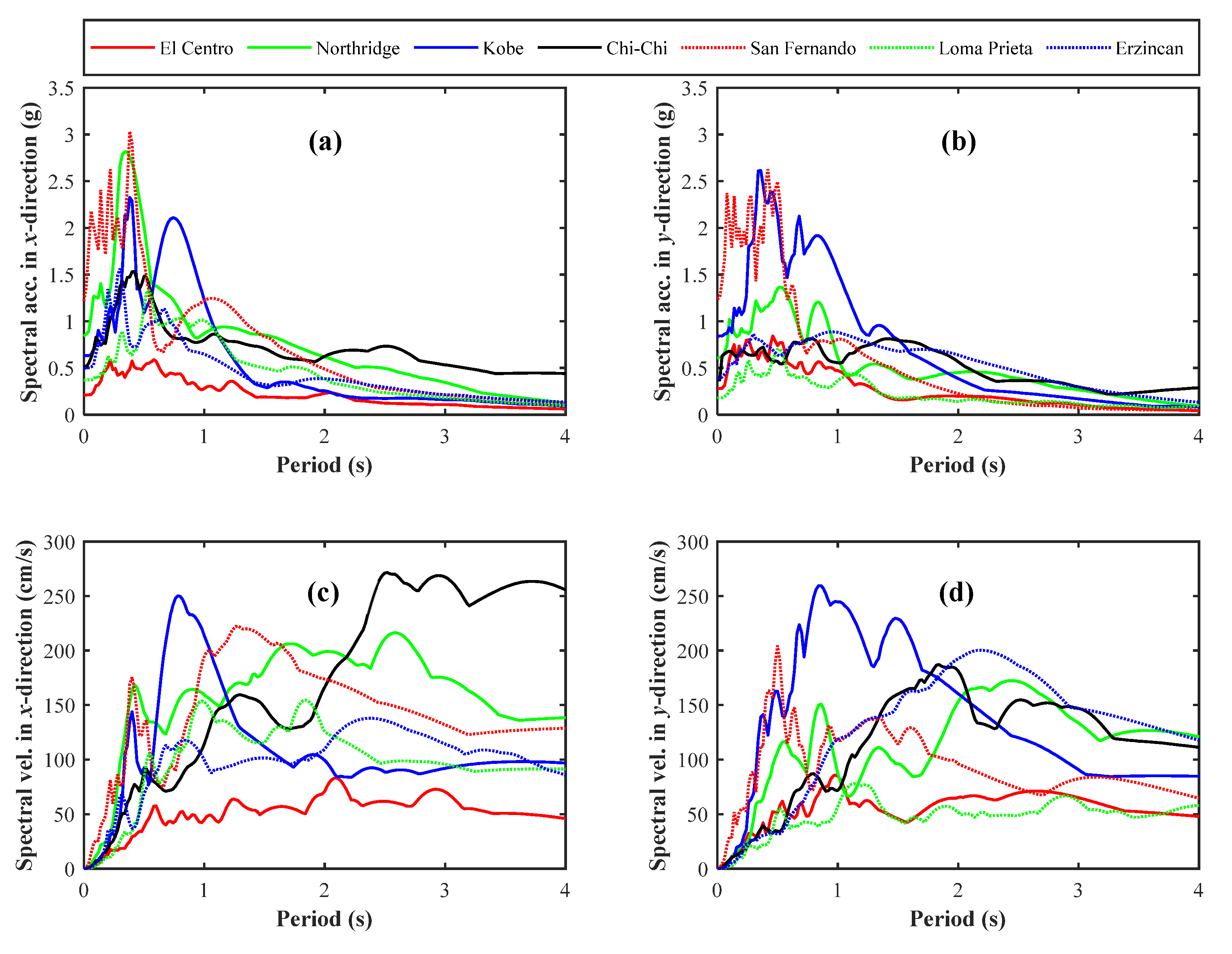
Figure 10.
Spectral acceleration, (a) and (b), and spectral velocity, (c) and (d), of the selected earthquakes in two directions.
Figure 10.
Spectral acceleration, (a) and (b), and spectral velocity, (c) and (d), of the selected earthquakes in two directions.

Figure 11.
The time-history responses of the Case-I building considering SSI effects under the Chi-Chi earthquake.
Figure 11.
The time-history responses of the Case-I building considering SSI effects under the Chi-Chi earthquake.

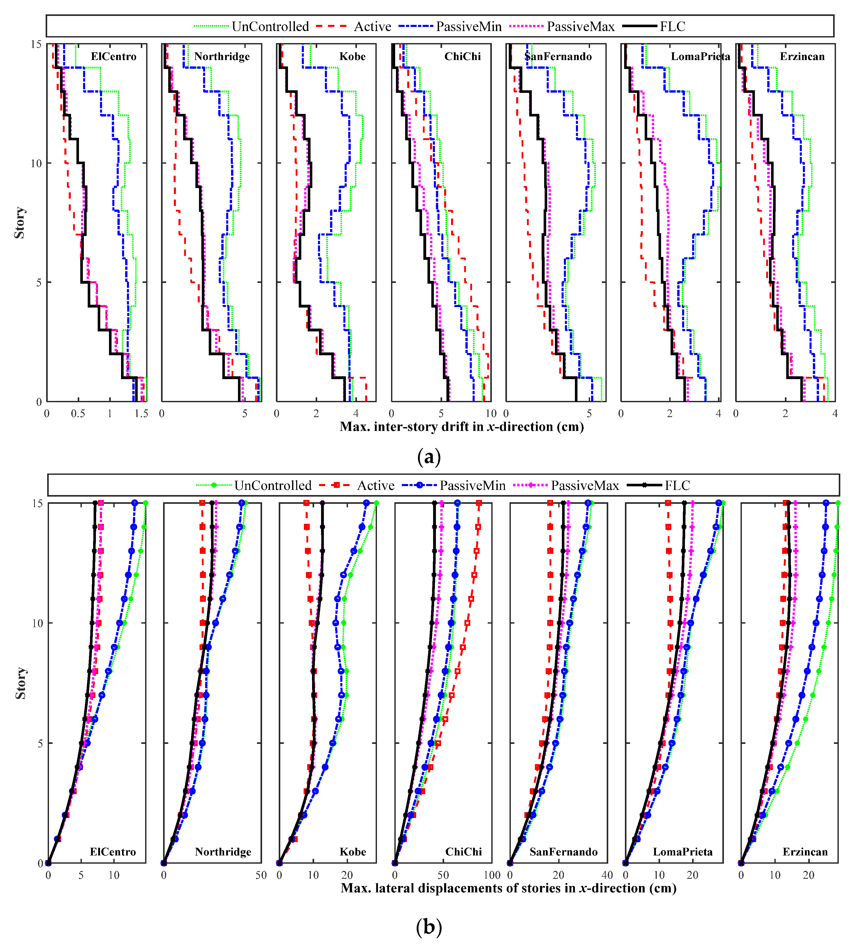
Figure 12.
Maximum lateral inter-story drifts, (a), and maximum lateral displacements, (b), of the Case-I building in the x-direction (soft soil).
Figure 12.
Maximum lateral inter-story drifts, (a), and maximum lateral displacements, (b), of the Case-I building in the x-direction (soft soil).

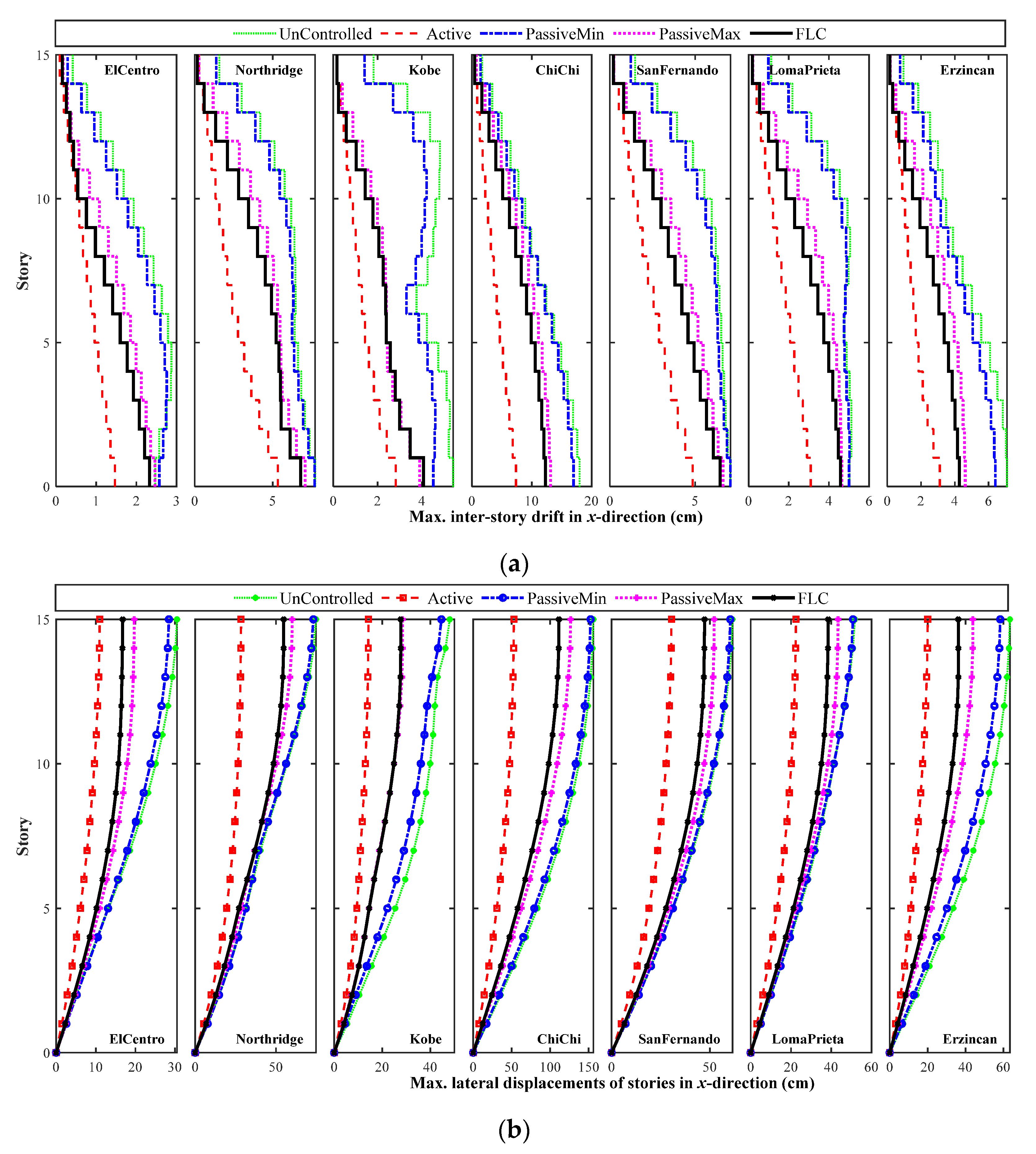
Figure 13.
Maximum lateral inter-story drifts, (a), and maximum lateral displacements, (b), of the Case-I building in the x-direction (rock base).
Figure 13.
Maximum lateral inter-story drifts, (a), and maximum lateral displacements, (b), of the Case-I building in the x-direction (rock base).

Figure 14.
Maximum lateral displacements of the Case-I building considering uncertainties in dynamic properties (soft soil). (a) and (d): Uncontrolled; (b) and (e): Active LQR; (c) and (f): FLC.
Figure 14.
Maximum lateral displacements of the Case-I building considering uncertainties in dynamic properties (soft soil). (a) and (d): Uncontrolled; (b) and (e): Active LQR; (c) and (f): FLC.

Figure 15.
Wireless vs. wired sensor network in case of power or signal line failure (Case I) in the x-direction, (a) and (b), in the y-direction, (c) and (d), and in the θ-direction, (e) and (f).
Figure 15.
Wireless vs. wired sensor network in case of power or signal line failure (Case I) in the x-direction, (a) and (b), in the y-direction, (c) and (d), and in the θ-direction, (e) and (f).

Figure 16.
Top floor displacements of two coupled buildings on a rock base with uncontrolled, (a), active control algorithm, (b).
Figure 16.
Top floor displacements of two coupled buildings on a rock base with uncontrolled, (a), active control algorithm, (b).


Figure 17.
Minimum Clear distance required to avoid pounding using active control with respect to different response weights.
Figure 17.
Minimum Clear distance required to avoid pounding using active control with respect to different response weights.

Figure 18.
Comparison of the responses using fuzzy logic control (FLC) and SPC algorithms under the Northridge earthquake.
Figure 18.
Comparison of the responses using fuzzy logic control (FLC) and SPC algorithms under the Northridge earthquake.

Figure 19.
The response of the adjacent buildings considering damage in the central building using SPC.
Figure 19.
The response of the adjacent buildings considering damage in the central building using SPC.


Table 1.
Dynamic properties of the springs and dashpots in the swaying, rocking and twisting directions for simulating soil–structure interaction (SSI) effects [32].
Table 1.
Dynamic properties of the springs and dashpots in the swaying, rocking and twisting directions for simulating soil–structure interaction (SSI) effects [32].
| Motion | r | Stiffness | Damping |
|---|---|---|---|
| Swaying | |||
| Rocking | |||
| Twisting |
| Parameter | Value | Parameter | Value |
|---|---|---|---|
| c0a | 50,300 (N s/m) | αa | 8700 (N/m) |
| c0b | 48,700 (N s/m V) | αb | 6400 (N/m V) |
| c1a | 8,106,200 (N s/m) | γ | 496 m−2 |
| c1b | 7,807,900 (N s/m V) | β | 496 m−2 |
| k0 | 5.4E-6 (N/m) | A | 810.50 |
| k1 | 8.7E-6 (N/m) | n | 2 |
| x0 | 0.18 (m) | η | 190 s−1 |
Table 3.
Characteristics of the selected earthquake records.
| Earthquake 1 | Station and Direction | Magnitude (Mw) | PGA (g) | PGV (cm/s) |
|---|---|---|---|---|
| 1940 El Centro | El Centro Array #9 270° | 7.2 | 0.21 | 31.3 |
| El Centro Array #9 180° | 7.2 | 0.28 | 30.9 | |
| 1994 Northridge | Sylmar—Olive View Med FF 360° | 6.7 | 0.84 | 129.6 |
| Sylmar—Olive View Med FF 090° | 6.7 | 0.61 | 77.5 | |
| 1995 Kobe | H1170546.KOB 090° | 7.2 | 0.63 | 76.1 |
| H1170546.KOB 000° | 7.2 | 0.83 | 91.1 | |
| 1999 Chi-Chi | TCU068 N | 7.6 | 0.37 | 264.1 |
| TCU068 E | 7.6 | 0.51 | 249.6 | |
| 1971 San Fernando | Pacoima Dam 164° | 6.6 | 1.22 | 114.5 |
| Pacoima Dam 254° | 6.6 | 1.24 | 57.3 | |
| 1989 Loma Prieta | Hollister—South and Pine 0° | 6.9 | 0.37 | 63.0 |
| Hollister—South and Pine 0° | 6.9 | 0.18 | 30.9 | |
| 1992 Erzincan | Erzincan—EW | 6.7 | 0.50 | 78.2 |
| Erzincan—NS | 6.7 | 0.39 | 107.14 |
1 Source: http://ngawest2.berkeley.edu/.
Table 4.
Maximum responses of the Case-I building using different control methods considering SSI effects (units in meters).
Table 4.
Maximum responses of the Case-I building using different control methods considering SSI effects (units in meters).
| Earthquake | Max. Response 1 | Uncontrolled | Active | Passive-min | Passive-max | FLC | |||||
|---|---|---|---|---|---|---|---|---|---|---|---|
| El Centro | 0.15 | (0.31) | 0.08 | (0.11) | 0.13 | (0.28) | 0.08 | (0.20) | 0.07 | (0.17) | |
| 0.14 | (0.28) | 0.05 | (0.07) | 0.13 | (0.26) | 0.06 | (0.14) | 0.06 | (0.13) | ||
| 0.006 | (0.011) | 0.004 | (0.004) | 0.005 | (0.010) | 0.002 | (0.005) | 0.002 | (0.005) | ||
| 1.52 | (2.72) | 0.54 | (1.94) | 1.16 | (2.58) | 1.39 | (2.41) | 1.72 | (2.78) | ||
| 2.18 | (3.49) | 0.89 | (2.96) | 2.01 | (3.41) | 1.59 | (3.30) | 1.83 | (3.50) | ||
| Northridge | 0.42 | (0.75) | 0.20 | (0.28) | 0.40 | (0.73) | 0.27 | (0.60) | 0.25 | (0.55) | |
| 0.26 | (0.48) | 0.10 | (0.22) | 0.24 | (0.48) | 0.15 | (0.41) | 0.16 | (0.40) | ||
| 0.037 | (0.074) | 0.014 | (0.026) | 0.035 | (0.071) | 0.020 | (0.053) | 0.020 | (0.053) | ||
| 5.37 | (11.71) | 2.19 | (8.41) | 5.07 | (11.54) | 4.29 | (10.97) | 3.60 | (10.19) | ||
| 3.77 | (7.21) | 1.37 | (6.17) | 3.15 | (7.00) | 3.12 | (7.15) | 3.01 | (6.92) | ||
| Kobe | 0.29 | (0.48) | 0.08 | (0.14) | 0.26 | (0.45) | 0.13 | (0.28) | 0.13 | (0.28) | |
| 0.27 | (0.46) | 0.10 | (0.17) | 0.25 | (0.43) | 0.14 | (0.34) | 0.14 | (0.34) | ||
| 0.008 | (0.014) | 0.003 | (0.004) | 0.007 | (0.013) | 0.003 | (0.008) | 0.004 | (0.009) | ||
| 6.24 | (7.41) | 1.18 | (5.63) | 5.33 | (6.45) | 2.95 | (7.05) | 3.29 | (7.40) | ||
| 5.54 | (9.54) | 1.80 | (8.09) | 4.78 | (9.08) | 3.14 | (8.93) | 3.12 | (8.69) | ||
| Chi-Chi | 0.66 | (1.56) | 0.87 | (0.53) | 0.64 | (1.53) | 0.48 | (1.27) | 0.41 | (1.11) | |
| 0.39 | (0.91) | 0.99 | (0.47) | 0.38 | (0.91) | 0.33 | (0.83) | 0.29 | (0.73) | ||
| 0.042 | (0.089) | 0.030 | (0.025) | 0.040 | (0.086) | 0.025 | (0.066) | 0.027 | (0.064) | ||
| 4.66 | (7.85) | 1.33 | (5.88) | 4.00 | (7.78) | 2.24 | (7.02) | 2.35 | (6.94) | ||
| 3.22 | (6.62) | 1.44 | (5.49) | 2.85 | (6.48) | 2.47 | (6.20) | 2.53 | (5.78) | ||
| San Fernando | 0.33 | (0.62) | 0.16 | (0.31) | 0.32 | (0.60) | 0.24 | (0.52) | 0.22 | (0.47) | |
| 0.15 | (0.19) | 0.05 | (0.12) | 0.13 | (0.17) | 0.08 | (0.17) | 0.08 | (0.17) | ||
| 0.017 | (0.030) | 0.009 | (0.015) | 0.016 | (0.029) | 0.010 | (0.021) | 0.010 | (0.020) | ||
| 5.28 | (11.44) | 2.65 | (11.79) | 4.83 | (11.30) | 4.05 | (10.92) | 3.76 | (11.06) | ||
| 3.95 | (12.12) | 2.87 | (11.94) | 3.38 | (12.40) | 3.56 | (12.17) | 3.55 | (12.91) | ||
| Loma Prieta | 0.29 | (0.52) | 0.13 | (0.22) | 0.28 | (0.51) | 0.20 | (0.43) | 0.18 | (0.39) | |
| 0.13 | (0.32) | 0.11 | (0.10) | 0.12 | (0.28) | 0.08 | (0.17) | 0.08 | (0.15) | ||
| 0.018 | (0.035) | 0.009 | (0.014) | 0.015 | (0.032) | 0.009 | (0.020) | 0.008 | (0.018) | ||
| 3.33 | (6.25) | 1.12 | (4.00) | 3.09 | (5.99) | 2.46 | (5.58) | 2.15 | (5.16) | ||
| 1.50 | (1.96) | 0.56 | (1.71) | 1.13 | (2.15) | 1.29 | (2.17) | 1.44 | (2.27) | ||
| Erzincan | 0.29 | (0.63) | 0.13 | (0.20) | 0.25 | (0.58) | 0.16 | (0.44) | 0.14 | (0.36) | |
| 0.41 | (0.77) | 0.19 | (0.28) | 0.39 | (0.76) | 0.27 | (0.64) | 0.25 | (0.57) | ||
| 0.030 | (0.066) | 0.016 | (0.023) | 0.029 | (0.064) | 0.019 | (0.049) | 0.018 | (0.045) | ||
| 2.94 | (6.21) | 1.14 | (4.88) | 2.21 | (5.93) | 1.94 | (4.92) | 1.84 | (4.42) | ||
| 4.00 | (6.00) | 1.57 | (5.20) | 3.89 | (6.05) | 2.77 | (6.08) | 2.91 | (5.76) | ||
1 Values in parenthesis are the corresponding responses for the rock base (no SSI).
© 2020 by the authors. Licensee MDPI, Basel, Switzerland. This article is an open access article distributed under the terms and conditions of the Creative Commons Attribution (CC BY) license (http://creativecommons.org/licenses/by/4.0/).
Share and Cite
MDPI and ACS Style
Azimi, M.; Molaei Yeznabad, A. Swarm-based Parallel Control of Adjacent Irregular Buildings Considering Soil–structure Interaction. J. Sens. Actuator Netw. 2020, 9, 18. https://doi.org/10.3390/jsan9020018
AMA Style
Azimi M, Molaei Yeznabad A. Swarm-based Parallel Control of Adjacent Irregular Buildings Considering Soil–structure Interaction. Journal of Sensor and Actuator Networks. 2020; 9(2):18. https://doi.org/10.3390/jsan9020018
Chicago/Turabian StyleAzimi, Mohsen, and Asghar Molaei Yeznabad. 2020. "Swarm-based Parallel Control of Adjacent Irregular Buildings Considering Soil–structure Interaction" Journal of Sensor and Actuator Networks 9, no. 2: 18. https://doi.org/10.3390/jsan9020018
Note that from the first issue of 2016, this journal uses article numbers instead of page numbers. See further details here.