
Wave Farms Impact on the Coastal Processes—A Case Study Area in the Portuguese Nearshore


Department of Mechanical Engineering, Faculty of Engineering, Dunarea de Jos University of Galati, 47 Domneasca Street, 800008 Galati, Romania
*
Author to whom correspondence should be addressed.
J. Mar. Sci. Eng. 2021, 9(3), 262; https://doi.org/10.3390/jmse9030262
Submission received: 1 February 2021
/
Revised: 23 February 2021
/
Accepted: 24 February 2021
/
Published: 1 March 2021
(This article belongs to the Section Ocean Engineering)
Abstract
:The aim of the present work is to identify the expected nearshore and offshore impact of a marine energy farm that would be implemented in the coastal environment of Portugal. Several layouts of Wave Dragon devices were considered, the distance between each system being gradually adjusted. By processing 27–years of combined wave data coming from the European Space Agency and ERA5, the most relevant conditions have been identified. The centre of each farm layout was set to approximately 3.5 km from the coast, where a more significant attenuation of wave heights in the middle of the target area was noticed, which can go up to 16% in the case of extreme events. From the analysis of the longshore currents, it was noticed that even an arrow farm layout defined by five systems may have a significant impact, by changing the peak or by smoothing the currents profile. Wave energy is an emerging renewable sector that can also contribute tocoastal protection and, therefore, the Portuguese coast represents a suitable candidate for this type of project.
1. Introduction
The erosion and accretion processes influence the stability of the coastal environment, but climate changes are a game changer since they put more pressure on these regions by adding extreme and sometimes highly unpredictable events. Based on satellite measurements, it was estimated that on a global scale, almost 28,000 km2 of eroded land was lost into the sea during 1984 and 2015, which is twice the surface of the newly created land [1]. This has an important implication for the near future, taking into account that almost 40% of the world population resides in these areas. The total length of the world coastlines is reported to be around 1,162,306 km, starting with Canada (202,080 km) and ending with Monaco (4.1 km) [2]. It is not realistic to consider viable solutions for protecting all these areas, so it is important to focus on some specific coastal sectors that may present interest for human activities (e.g., sandy beaches) and are difficult to maintain. Included in this category are areas facing the ocean environment, such as those in Portugal, which are well known for surfing activities, and during a storm event, significant wave heights can reach 7 m [3,4].
A first step in planning a coastal protection strategy is to understand the severity of the marine conditions, which can be done through the use of some modern technologies, namely satellite missions [5,6,7]. These types of measurements are known for their accuracy and global coverage, however, a drawback is the low spatial/temporal resolution, which can be compensated by combining data from multiple missions [8]. For wave energy assessment and coastal applications, these data provide limited information since they indicate only the wave heights, but even so, there are methods to obtain the wave period by considering wind speed conditions [9]. For the Portuguese coastal area, the satellite data are used for various applications, such as water quality [10,11], calibration of wave models [12,13,14] or evaluation of renewable energy resources [15,16,17].
The Portuguese nearshore covers a significant part of the Iberian Peninsula, and, therefore, coastal protection represents an important issue. Almost 12,500,000 m3 of sand was used between 1990 and 2017 to consolidate some beach areas (around 20 sectors) that do not exceed an area of 75 km. On the other hand, it has been identified that the hard engineering solutions implemented in this region were not the best solution, since they accelerated the coastal erosion by disrupting the natural flow of the sediments [18]. In the past, safety issues were considered important with impact studies not taken into account, but nowadays through the use of computational methods, it is possible to tackle the existing problems in a more sustainable way [18]. The Portuguese shoreline (sandy areas) retreat by a rate of 1 to 5 m/year, with affected areas from the Algarve region (south) and the west coast including Aveiro and Costa da Caparica. The present strategy is to maintain and adjust the existing coastal infrastructure, but in the long term, this seems to be a rigid approach. The sea level has increased by a rate of 2.1 mm/year, with an expected difference of 47 cm by 2100 (reported to 1990). This implies that the intensity of the wave conditions will go up, especially as regards the western shoreline of the Portuguese continental coastal environment [19].
The coastal defence through wave farms represents a new concept that emerged in recent years [20,21,22]. This seems to be an attractive solution since it involves floating wave energy converters (WECs) capable of adjusting to sea-level changes and extreme marine conditions, including various types of configurations that can go from point absorbers to terminator devices, like for example, the Wave Dragon considered in the present work [23,24,25]. It is important to mention that at this moment, the WECs are not yet competitive from an economical point of view and, therefore, by finding a niche like coastal protection, the integration with harbour infrastructure or in mixed wind–wave projects can accelerate the development of this renewable sector [26,27,28]. Various case studies involving some wave farms were implemented for the Portuguese coastal area, such as the Pelamis system considered by Palha et al. [29] and Rusu and Soares [30]. The results clearly show that by using this soft engineering approach, it is possible to obtain suitable coastal protection for some targeted coastal sectors. However, some projects are no longer operational, including the Pelamis, although this was the world’s first attempt at a commercial wave farm [31]. In some other studies [32,33,34], generic or hybrid energy farms were used to assess the variations of the nearshore wave climate, including the longshore currents. Based on these results, it was found that a high absorber wave farm located 7 km from the shore may decrease the wave heights by 1 m near the coastline.
Compared to some previous studies, the present work is defined by the following novel elements:
- (a)
- Long term satellite and reanalysis data are processed and analysed;
- (b)
- A wave farm defined by the Wave Dragon system is implemented in the Obidos sector, in the Portuguese continental nearshore;
- (c)
- Various spatial configurations are defined and analysed.
2. Materials and Methods
2.1. Target Area
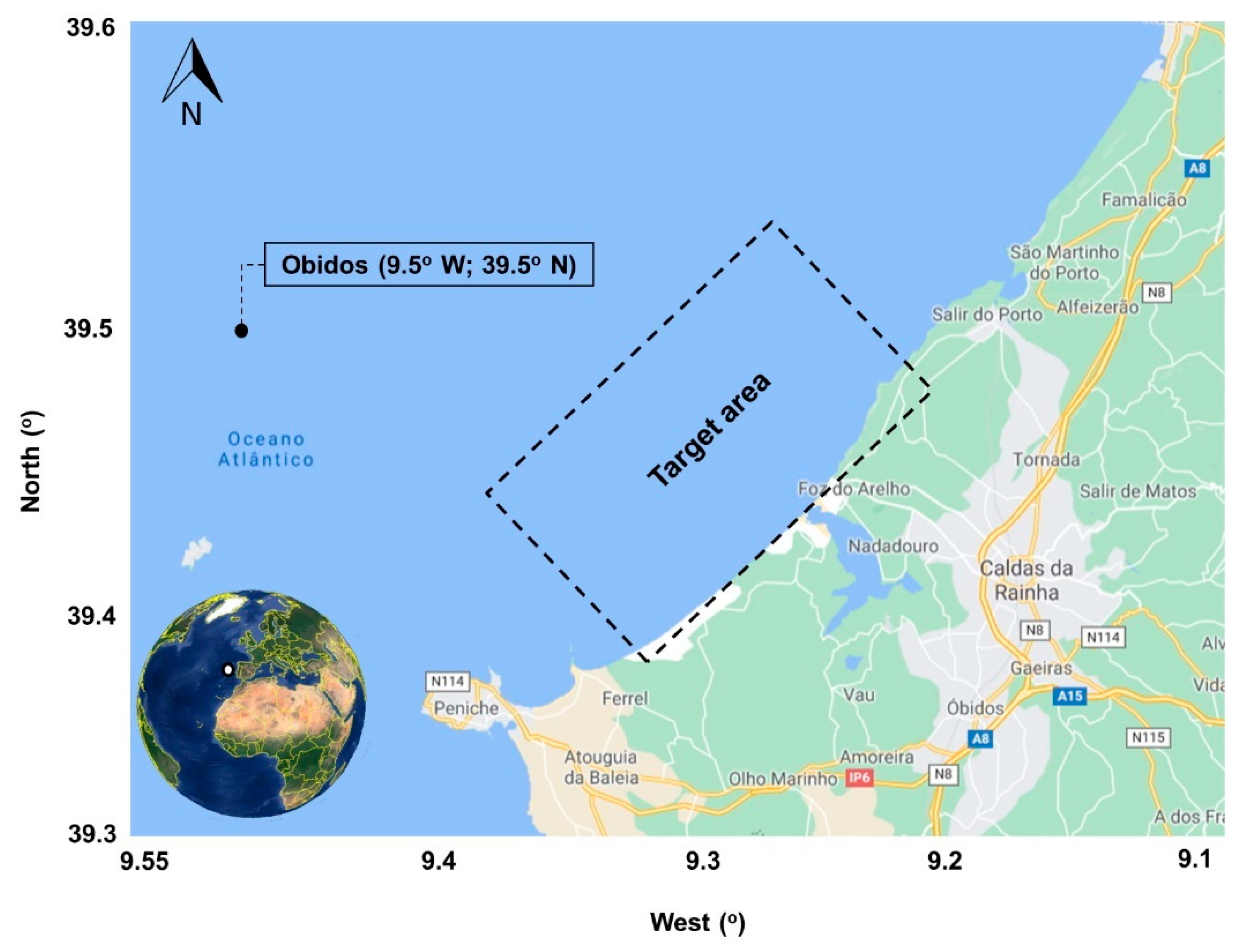
In Figure 1, the study area is presented. This is in front of the Óbidos lagoon, more precisely between the Peniche Peninsula (south) and Sao Martinho do Porto (north. The shoreline orientation is 315° (nautical convention–clockwise), and it is important to mention that the existing lagoon is separated from the ocean by a 1 km sand spit (of 100 m width), that is frequently subjected to high waves (ex: 2.5 m) and strong semi-diurnal tide (ex: 1–4 m) [35]. To obtain a sand spit, some special criteria need to be met, namely: (a) the oblique incident waves are dominant; (b) a large volume of sediment is provided by a river or from coastal cliffs. The wave conditions are involved in the sand accumulation, while subsequently, the longshore currents influence the variation of the spit sand area (area and elongation) [36]. According to Oliveira et al. [37], the hydrodynamics of Obidos lagoon is strongly influenced by the wave conditions, which during wintertime, carry sediments and the inlet is subjected to accretion, while during summertime, a reverse trend is noticed. In this way, during wintertime, the tidal amplitude is reduced by almost 50% while flood dominance increases. Nevertheless, the instability of this inlet represents a major issue for the water quality and sediment transport, and as a consequence, various strategies have been implemented over time (dredging, guiding walls, inlet reposition, sandbags during winter) [38].
2.2. Wave Data
2.2.1. European Space Agency (ESA)
Satellite measurements represent an important source of information for marine areas, this being the case of the ESA Sea State Climate Change Initiative–Sea State (CCI-SS) project, which aimed to provide a better picture of the climatological changes. This project combined data from multiple satellite missions into a merged system capable of delivering monthly significant wave height values (Hs), available on a global scale. The data available covers the interval 1991–2018 and is based on several altimeters’ inputs such as ERS-1, Topex, Envisat, GFO, CryoSat-2, Jason-1 and SARAL. Various products are available and, in this study, a monthly gridded satellite altimeter providing significant wave heights (Level 4 data) with a spatial resolution of 1° × 1° was used. This product was constantly improved through filtering and corrections, and a major advancement related to the implementation of an Empirical Mode Decomposition method capable of handling the sea surface height [39]. A reference point (9.5° W; 39.5° N) was defined for the Obidos target area (see Figure 1), in order to identify the most relevant wave heights that may occur in this coastal environment. A limitation of this type of measurement is that it only provides information for the Hs parameter, but this can be compensated by adding some other sources, such as reanalysis data.
2.2.2. ERA5
The aim of ERA5 is to replace the ERA–Interim database that was produced by the ECMWF (European Centre for Medium–Range Weather Forecasts). At this point, ERA5 covers the interval from 1979 to the present, but the final goal is to extend this period up to 1950. Compared to some previous projects, several improvements were made including the implementation of a 4D–Var data assimilation method defined by 137 hybrid sigma/pressure (model) levels. The wave parameters were obtained from a numerical model that uses spectra defined by 24 directions and 30 frequencies, defined by a horizontal resolution of 0.36 degrees. Compared to ERA–Interim where 25 parameters were generated, in ERA5 the number increased to 46 [40]. For the present work, the wave characteristics were assessed in an offshore location close to Obidos (Figure 1). ERA5 provides data on various spatial resolutions, and for the present work, a grid of 0.25° × 0.25° was used to extract the time series corresponding to the Obidos site. Data corresponding to the same period covered by the ESA measurements was processed, and in this case, four data per day were considered (00–06–12–18 UTC). However, the wave characteristics evaluated this time were the mean wave direction (Dir), mean wave period (Tm) and the significant wave height (Hs), with the first two wave parameters not available in ESA data.
2.3. ISSM and Case Studies
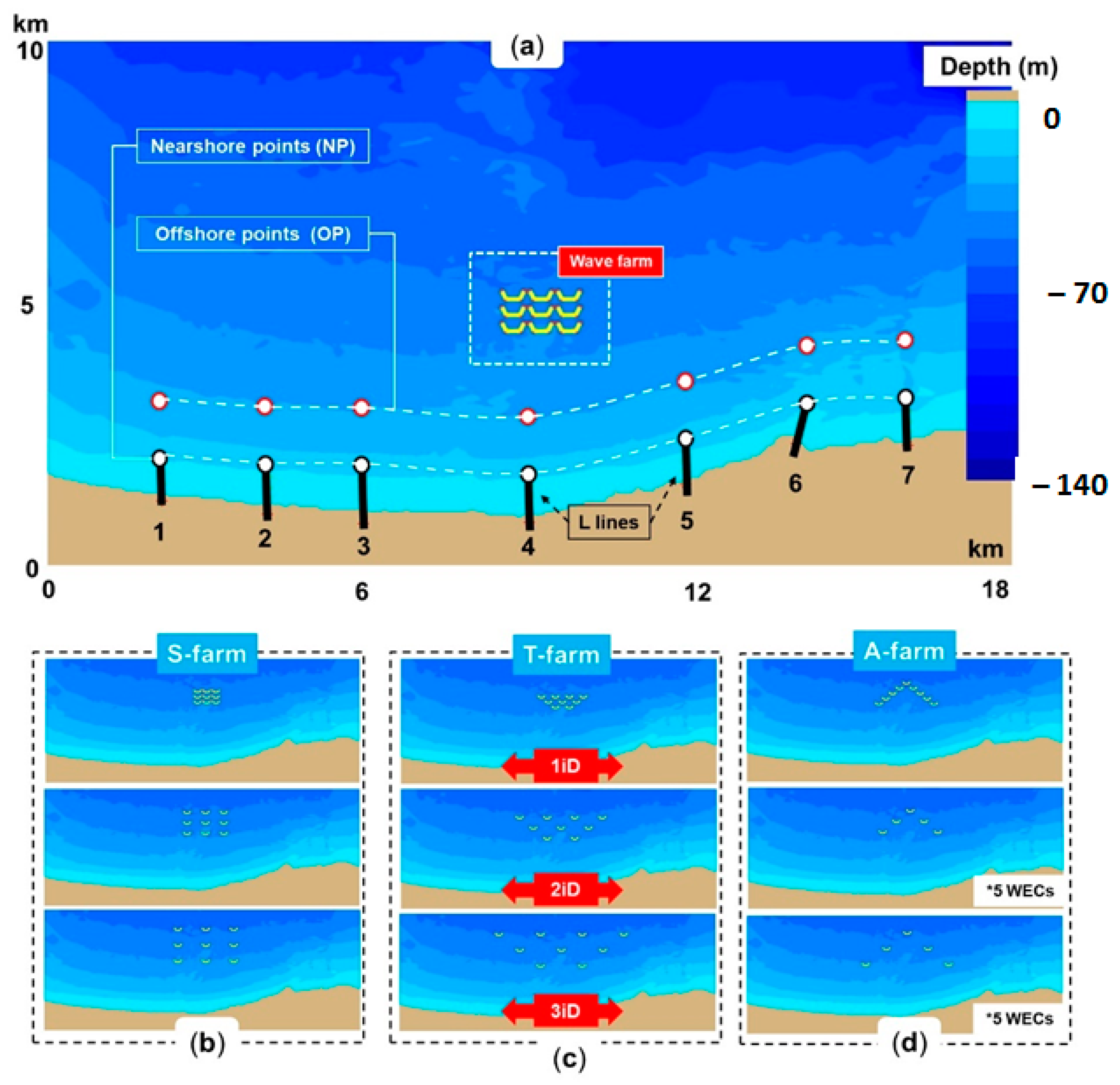
The Interface for SWAN and Surf Models (ISSM) was used to evaluate the coastal impact of the wave farms considered. This is a combination of the SWAN spectral wave model [41,42], which simulates the nearshore wave propagation, and the Navy Standard Surf Model (denoted as Surf), which is used to evaluate in more detail the nearshore processes, in particular the longshore currents [43,44]. It is important to mention that the SWAN model was already validated for the Obidos area, the results showing a good agreement with in situ measurements [45]. Figure 2 presents the Obidos computational domain, with Figure 2a showing it was defined by a rectangle of 10 by 18 km and by a maximum water depth of 140 m.
A wave farm was placed in the middle of this area, at approximately 4 km from the shore (reported to the centre of the farm), the expected impact being quantified by some nearshore (from NP1 to NP7) and offshore points (OP1 to OP7), while the profiles of the longshore currents were assessed by considering the L–lines. Table 1 shows the water depths associated with each reference point (nearshore and offshore). Higher values are noticed at the points located in the central area, with the values in the ranges of 10.02–16.71 m (for nearshore points) and 18.27–27.61 m (for offshore points).
The Wave Dragon system was considered as a reference for this wave farm, being defined by a length of 260 m and a width of 150 m, these values defined a 1iD (one dimension) wave farm. More precisely, in a 1iD farm, the distance between devices along the x-axis (parallel to shoreline) was the length of the Wave Dragon while for the y-axis (perpendicular to shore), the width of this system was used. In the 2iD and 3iD configurations, the initial values from 1iD were multiplied by 2 and 3, respectively. The transmission coefficient of each wave generator was set to 0.68, which meant that only 32% of the incoming waves were retained. This set–up was in the line with some other works [46,47] that considered a similar approach and wave converter. At this point, it has to be highlighted that in the present work, the wave energy extraction was modeled using transmission coefficients, while the frequency dependence of the wave energy harvesting was not taken into consideration.
However, wave energy converters do not extract energy equally from all frequencies. Thus, ignoring this property of the wave energy converters may overestimate the impacts they will have on the wave field in the lee of the arrays. See for example [48] and also a similar study [49]. On the other hand, the objective of the present work was to assess the coastal impact of various marine energy farm configurations and not to model in a very accurate way the wave energy extraction for a certain device. For this reason, the approach using transmission coefficients was considered.
Following the work of López–Ruiz et al. [50], three wave farm layouts were designed, namely: (a) square farm (S-farm); (b) trapeze farm (T-farm); (c) arrow farm (A-farm). The configurations of these farms are presented in Figure 2, each layout including 9 systems, except for the A-farm (2iD and 3iD) where only 5 systems were used. This adjustment was made because the growth rate of the A-farm significantly exceeded the size in comparison with the S and T configurations, being possible to avoid some unrealistic situations (ex: 3iD layout–systems located on land). More details about the SWAN model set–up are presented in Table 2, where: ∆x and ∆y–are resolutions in the geographical space, ∆θ–the resolution in the directional space, nf and nθ–the number of frequencies and directions in the spectral space. In order to better account for the physical processes depending on the resolution in the frequency space, a number of 34 frequencies were considered in the SWAN model simulations. This defined a high grid resolution in frequency–space between the lowest discrete frequency (flow) and the highest discrete frequency (fhigh). However, this resolution was not constant, since the frequencies were distributed logarithmically. Following the indications provided in [41], the values of the frequency limits were selected as flow = 0.03 Hz and fhigh = 1.1 Hz.
At this point, it has to be highlighted that diffraction is particularly important in such evaluations of the coastal impact induced by marine energy farms. This process has the effect of spreading energy laterally and may yield smoother wave fields in the lee of the arrays. As shown in Table 2, together with other physical processes relevant in intermediate and shallow water, such as bottom friction, depth-induced wave breaking and triad wave–wave interactions; diffraction was also activated in the model simulations. On the other hand, it is known that the SWAN model does not properly handle diffraction in harbours or in front of reflecting obstacles.
However, behind the breakwaters of a down–wave beach, the SWAN results appeared to be reasonable enough. Furthermore, in order to increase the convergence of the diffraction computations, an extra measure was taken in the model settings. This consisted of smoothing the wave field for the computation of the diffraction parameters (the wave field remained intact for all other computations and output). This was done with repeated convolution filtering as presented in the SWAN user manual [51].
3. Results
3.1. Evaluation of the Wave Characteristics
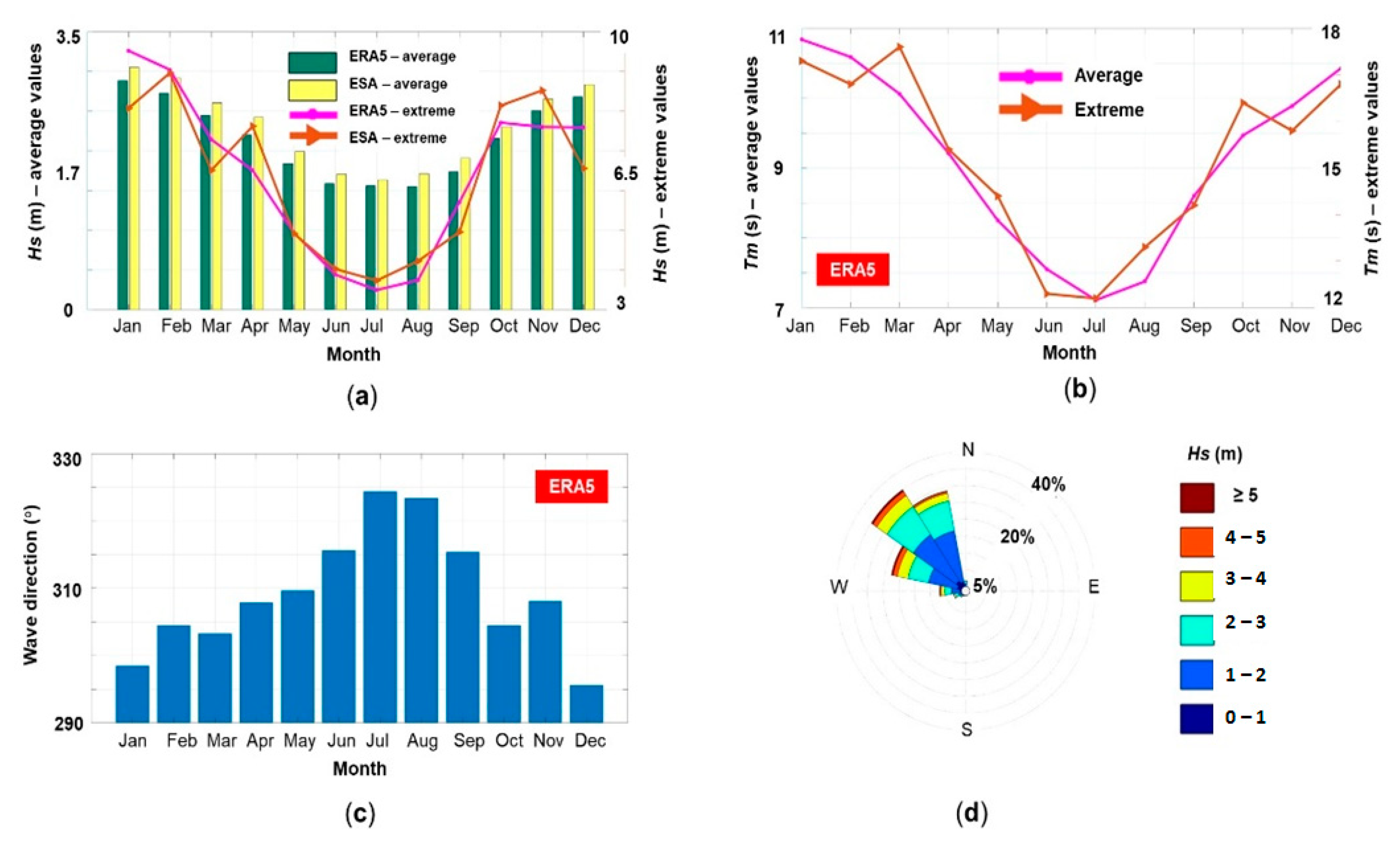
Figure 3 provides a general picture of the wave conditions from the Obidos area, by considering 27–years of combined satellite measurements and ERA5 data. In general, for the assessment of the wind and wave conditions, it is recommended to use at least 10–years of data [53], with a large number of satellite data indicating the progress in this field. By looking at these results, we noticed that definitely, the wave conditions indicated a seasonal fluctuation, where for the Hs and Tm parameters, much higher values were noticed during the wintertime (October–March), while for the wave direction, the values increased during the summertime (above 310°). From the analysis of the Hs data (Figure 3a), the ESA results were higher than those from ERA5, especially in the case of the average values reported in the range of 1.64–3.05 m (July and January). As for ERA5, a similar pattern occurred, with values of 1.55 and 2.9 m (August and January). For the extreme values, there was a good agreement between the two datasets for February (9.04 m), May (4.94 m) and June (3.89 m), respectively. Higher values were provided by the ESA project during April (7.62 m), October (8.14 m) and November (8.52 m), while for January (8.07 m) and December (6.56 m), the values dropped below the ERA5 data. Figure 3b presents the evolution of the Tm parameter (only ERA5), which on average can go from 7.1 to 10.84 s (summer to winter), while the extreme values indicated a maximum of 17.6 s (in March) with a minimum of 12.2 s noticed between June and August, respectively.
The dominant wave direction (Figure 3c) was in the range of 295.6–324.4°, with lower values occurring in January and December, compared to July and August when the values significantly increased. From the analysis of the wave roses (Figure 3d), we could see that the waves were coming from the north-west sector, being oblique to the Obidos coastal sector, confirming the formation of the local sand spit.
To run the numerical simulations in a stationary mode, some case studies (CS) needed to be defined and in Table 3, such CS were selected that combined the ESA (Hs values) and the ERA5 (Tm and Dir values) data. Relevant extreme conditions were selected from winter and summer (February and July), also including a January sea state that was considered representative for winter (average conditions).
At this point, it has to be highlighted that Figure 3 presents the wave statistics based on information coming from the two databases considered (ERA5 and ESA). The reason for considering two different sources is that in this way, a more realistic picture of the wave conditions was provided. The satellite measurements presented more accurate results than the ERA5 model, with these also using data assimilation techniques to improve their hindcast. From this figure, we can define the average and extreme values corresponding to the seasons and to each individual month. In a first approach, in the present work, the winter extreme and average conditions were selected and they corresponded to the CS1 and CS2 case studies. The reason was that the extreme (CS1) corresponded to the most energetic situation that could be encountered while the winter average corresponded to the most representative conditions for the wintertime, which was also very representative for spring and autumn. Additionally, the extreme summer conditions were also considered (CS3), because these were high wave conditions that may have a significant impact on the nearshore. A fourth situation was also considered corresponding to the summer average wave conditions, but since the wave energy was quite low in this situation, this case was not considered relevant in relation to the objectives of the present work.
In Table 4 the Hs values are presented. These are illustrated by the nearshore/offshore points for all the case studies, in the absence of the wave farm. As expected, the CS1 scenario indicated the highest values that go from 8.01–8.42 m (offshore) to a minimum of 6.7 m near the coastline. The attenuation was more severe near the point NP7, compared to the central part (ex: NP5) where the waves could reduce by 0.3–0.6 m. Compared to CS1, in the case of the CS2 and CS3 scenarios, some nearshore points indicated slightly higher values than the offshore ones, this being the case of NP1–3.3 to 3.38 m (CS3) or NP6–2.87 to 2.97 m (CS2), respectively.
The wave direction indicated how the wave energy was distributed in the geographical space, being also directly related to the generation of the longshore currents. Table 5 presents this distribution (no wave farm), for which we can notice that regardless of the case study, the direction was in the range 293–322°. For CS1 and CS2, the wave direction increased from offshore to nearshore in the case of the group points 1–2–3–4, while a reverse pattern was noticed for the remaining points. The CS3 scenario indicated no significant variation in the case of the group points NP1–NP3, while the differences started to increase from NP4 (−2°) to NP7 (−14°), respectively.
The wave-induced forces (N/m2) provided important information concerning the wave intensity acting on a particular WEC system (ex: mooring lines) or how a coastal structure would be affected. Table 6 presents the distribution of this characteristic (no wave farm), from which we could notice that higher values corresponded to the nearshore points. The values of the wave forces strongly depended on the severity of the wave conditions, this being the case of CS1 when the offshore points indicated wave forces with values in the range of 5.45 (OP2) and 46.2 N/m2 (OP6).
Going further to the nearshore points, the value of the wave forces could easily jump to 70.9 N/m2 (NP1) or 91.5 N/m2 (NP6), while a minimum value of 7.86 N/m2 wads expected near NP5. The CS2 and CS3 conditions indicated relatively similar values for the offshore area, where much higher values were expected close to OP6–OP7 (ex: 4.98 N/m2), while close to the nearshore a maximum value of 16.8 N/m2 corresponded to NP6.
The wave action was in charge of the suspended sediments and through the orbital velocity near the bottom (Ubot) these particles were carried to the shoreline. In Table 7, a general picture of this parameter is provided (no farm), and from the information provided by CS1, we could notice that the sediment transport was initiated in the offshore area (Ubot > 2 m/s) while close to the shore, this process was accelerated with reported values in the range of 2.74–3.17 m/s. In the case of CS2–CS3, the offshore conditions seemed to have a limited impact on the sediment circulation, with much higher values being encountered by the nearshore points (ex: 1.46 m/s). The Hjulström curve [54] is designed to establish the sediment pattern corresponding to different sediment types, with a mention that for this work, the sand appears to be the dominant one, taking into account the presence of the Obidos sand spit [35]. For velocities exceeding 0.1 m/s, the erosion processes were dominant, regardless of the sand sediment size (fine–medium–coarse), this being reflected by all the points considered in Table 7. More than this, the higher Ubot values could easily contribute to the erosion and transport of coarse material, such as cobbles (64–256 mm).
3.2. Coastal Impact of the Wave Farms
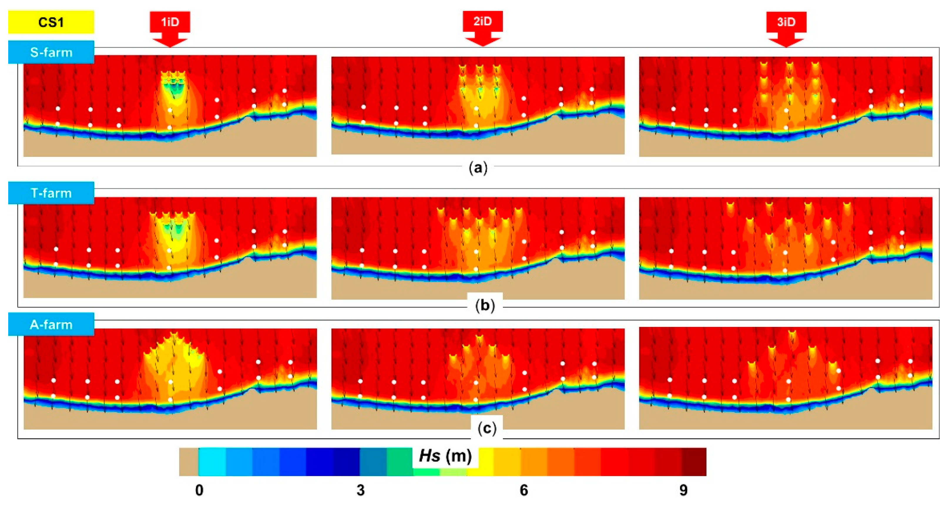
Figure 4 illustrates the spatial distribution of the significant wave height for the CS1 scenario. The shielding effect generated by the wave farms was visible in all cases, being more obvious for the 1iD scenario. By combining this information with the ones corresponding to the OP and NP points, we could obtain a more comprehensive picture of the expected impact. For example, in the case of the S-farm, the offshore points OP1 and OP7 indicated no variations, which was expected by looking at their position, the size of the farms and the wave direction. For the reference points NP2, NP3 and NP4, the Hs values constantly decreased as we went from the 1iD to the 3iD scenario, but for the NP4, a 3iD configuration (6.35 m) was less efficient than a 1iD (6.08 m) or 2iD (5.99 m) layout. Since a T-farm is wider than an S-farm, this provided better protection for the point NP2 (from 8.36 to 8.09 m–3iD), and for the points NP3 and NP5. Nevertheless, for the point NP4 (located in the center of the target area), an S-farm performed much better.
Going to the nearshore points, the presence of these wave farms would significantly attenuate the wave heights in the central part (NP3, NP4 and NP5), with a mention that for the point NP4, some particular configurations were used, namely: 2iD for the S-farm; 1iD and 2iD for the T-farm; 1iD for the A-farm. For the point NP5, the Hs parameter could decrease from 8.15 m to a minimum of 7.55 m (S-farm/3iD), 7.43 m (T-farm/3iD) or 7.45 m (A-farm/3iD), with a mention that for the A-farm only, 5 WECs were included.
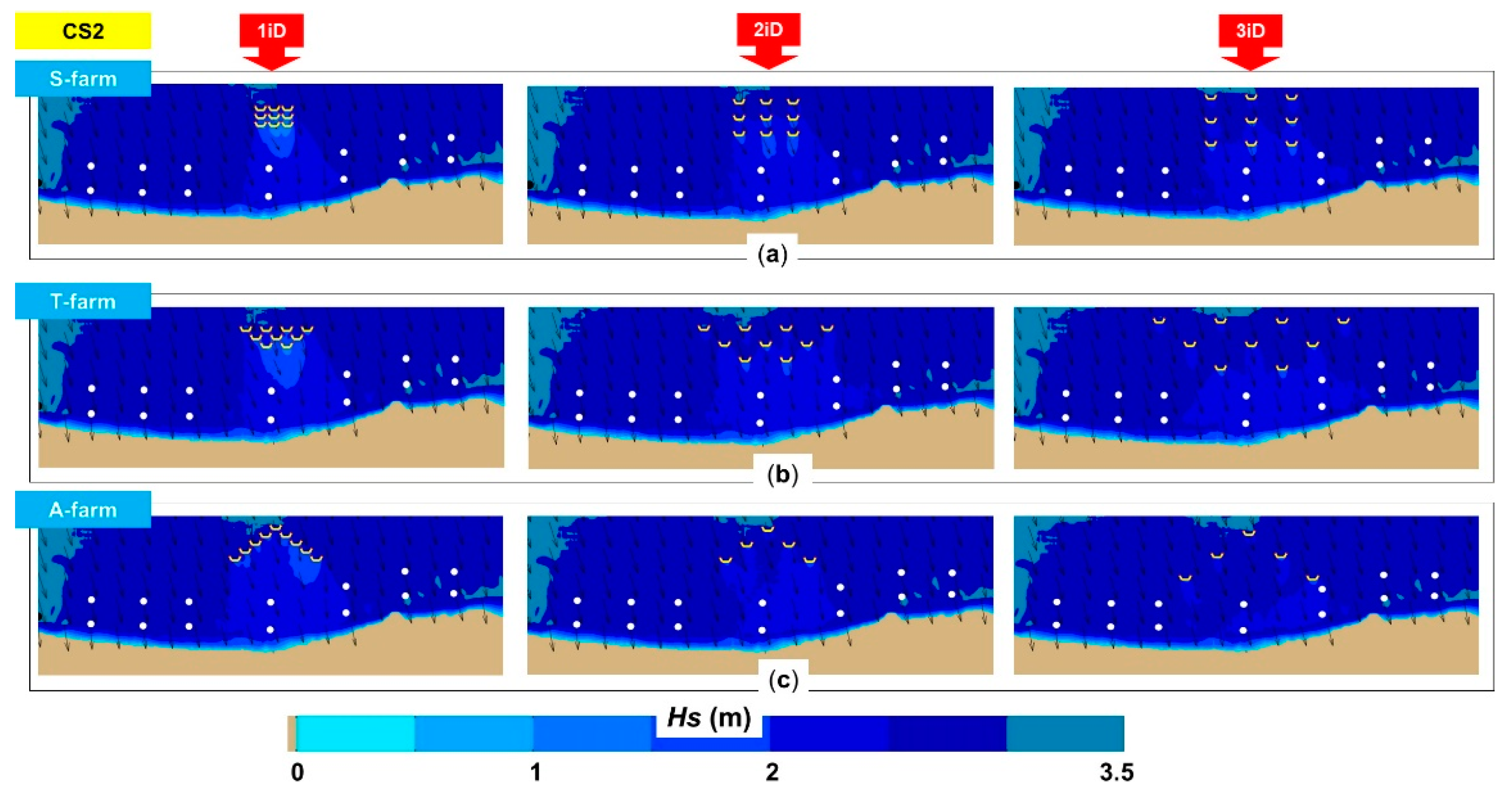
For the CS2 scenario (Figure 5), the impact of the wave farms was more visible behind the last WEC line which gradually extended to the shoreline. In this case, the results showed that the T-farm/3iD provided some protection for the point NP7 (indicating a Hs decrease from 2.84 to 2.78 m), in the condition when this was located at approximately 8.5 km from the centre of the farm. The point NP5 indicated, in this case, better protection than NP3, which was mainly related to the direction of the waves. The Hs values could decrease from 2.76 m to: S-farm (2.54–2.45–2.39 m /1iD to 3iD), T-farm (2.48–2.39–2.4 m) or A-farm (2.44–2.55–2.43 m).
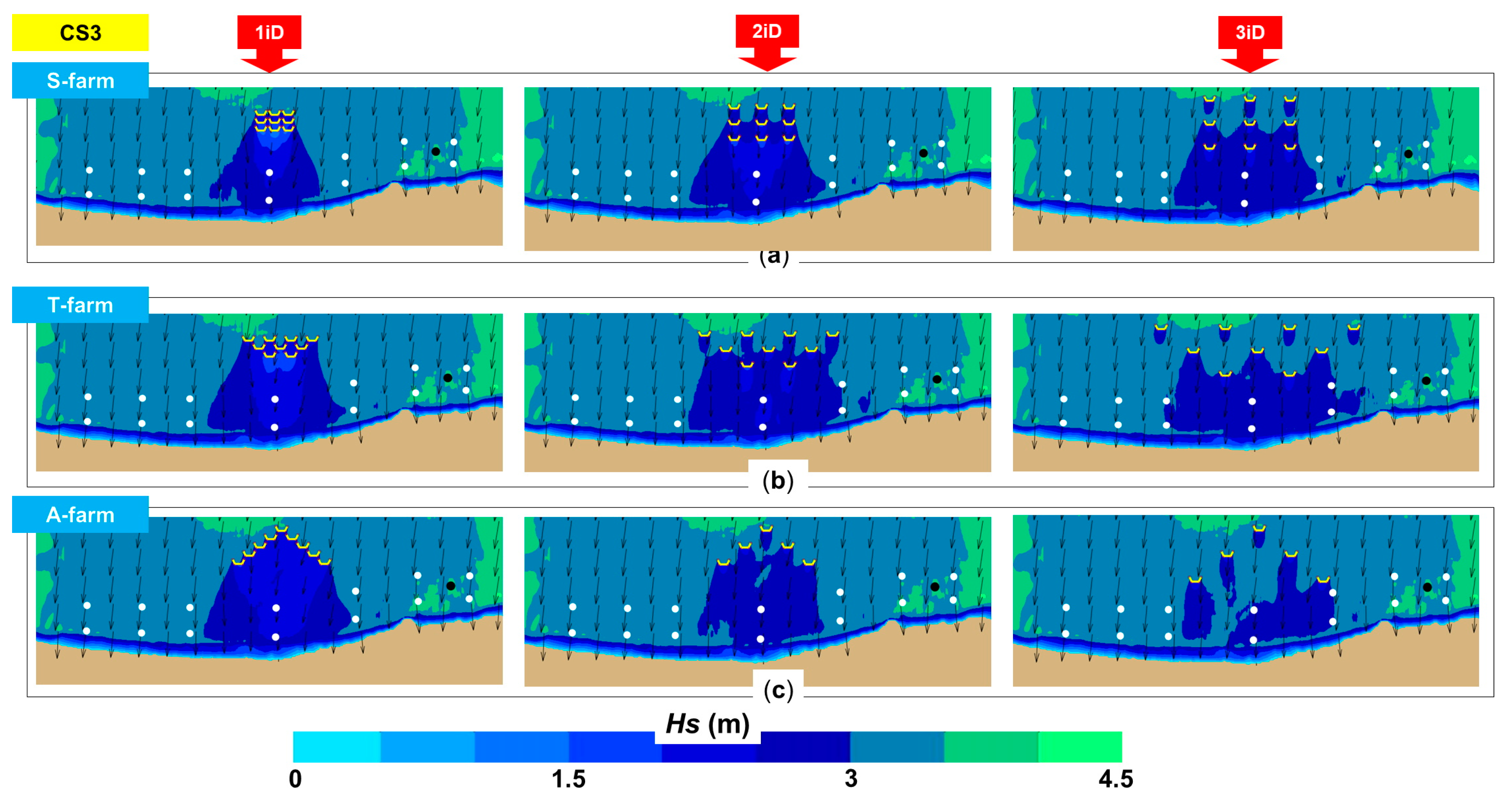
Figure 6 presents the impact of the wave farms for the CS3 scenario, where a Hs value of 3.7 m and a wave direction of 324° were considered for the SWAN simulations. Close to the shoreline, the influence of the farm was minimal for the points NP1 and NP7, while in the case of NP2 and NP6, a T-farm configuration (3iD) reduced the waves from 3.31 to 3.01 m, and from 3.65 m to 3.57 m, respectively. The farm protected the central part of the target area (point NP4), with noticed attenuations of 0.62 m–S-farm/2iD, 0.68 m–T-farm/1iD or 0.7 m–A-farm/1iD, respectively. For the 3iD configuration, the differences observed between different farm configurations were very small, except for point NP4, where the A-farm was less efficient (ex: 2.9 m compared to 2.62 m–S-farm).
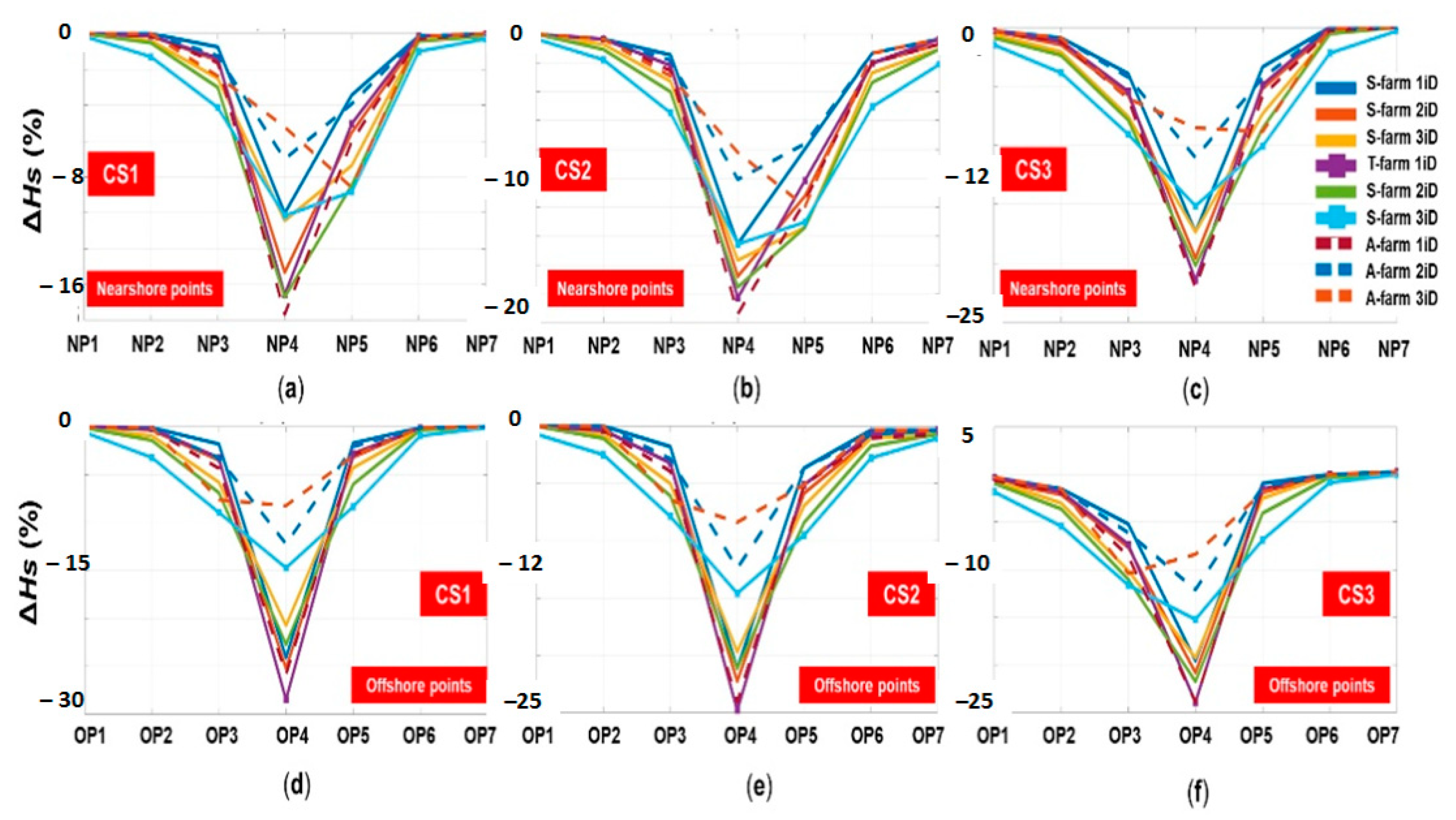
The Hs differences (in %) reported between the no farm and the wave farm scenarios are presented in Figure 7. From this, we can notice that most of the values were negative, which meant that the wave farm would reduce the wave heights in some way, with some positive values noticed for CS3-offshore points (Figure 7f), which were, in fact, insignificant. Regardless of the scenarios, point 4 indicated the maximum Hs attenuations that could go up to 30% (offshore) or 20% (nearshore), respectively. For the CS1 scenario (nearshore points), an A-farm/1iD configuration was more efficient indicating a maximum attenuation of 16% compared to 10% for the S-farm. For the 2iD and 3iD configurations, the maximum attenuation was similar for the T-farm and A-farm, with a mention that the T-farm had a slightly higher impact on the points NP3 and NP5. A similar pattern was noticed for the scenarios CS2 and CS3, with a mention that for CS2, the impact of the farms was also visible for NP6 (ex. 5.1%–T-farm/3iD).
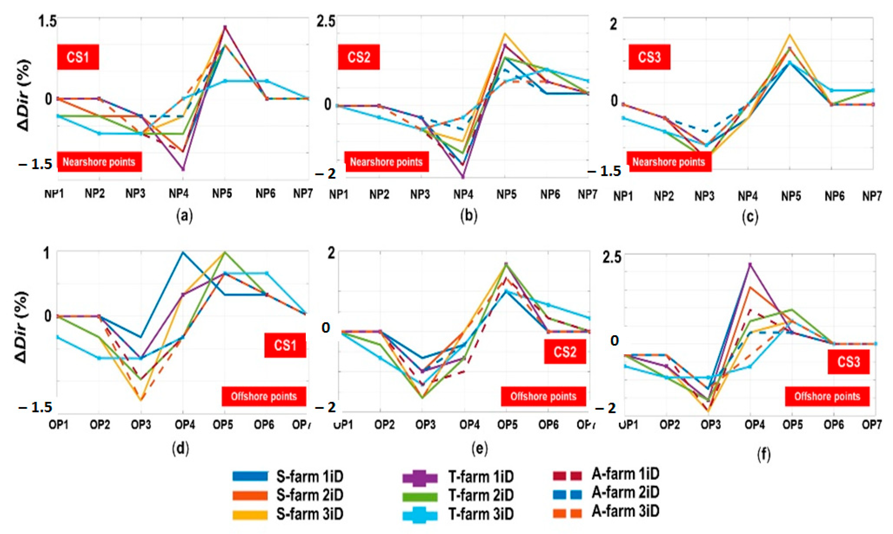
The presence of the farm clearly influenced the direction of the waves, as we could notice from Figure 8. For the offshore area, the points OP2 and OP3 indicated negative values, while an opposite pattern was noticed for the points OP4, OP5 and OP6. For CS2, the points OP3 and OP5 indicated the highest peaks of 1.7%, while for CS3, the peaks corresponded to OP3 (1.9%) and OP4 (2.2%), respectively. As for the nearshore points, the differences did not exceed 0.64% for NP3, these differences being mainly generated by the 3iD configurations. On the other hand, for the point NP4, a 1iD configuration had a higher impact, with an expected variation of 1.3% for the T-farm. For scenarios CS2 and CS3, the point NP5 indicated a positive peak (2%) while the negative peak changed between NP4 (2%) and NP3 (1.2%).
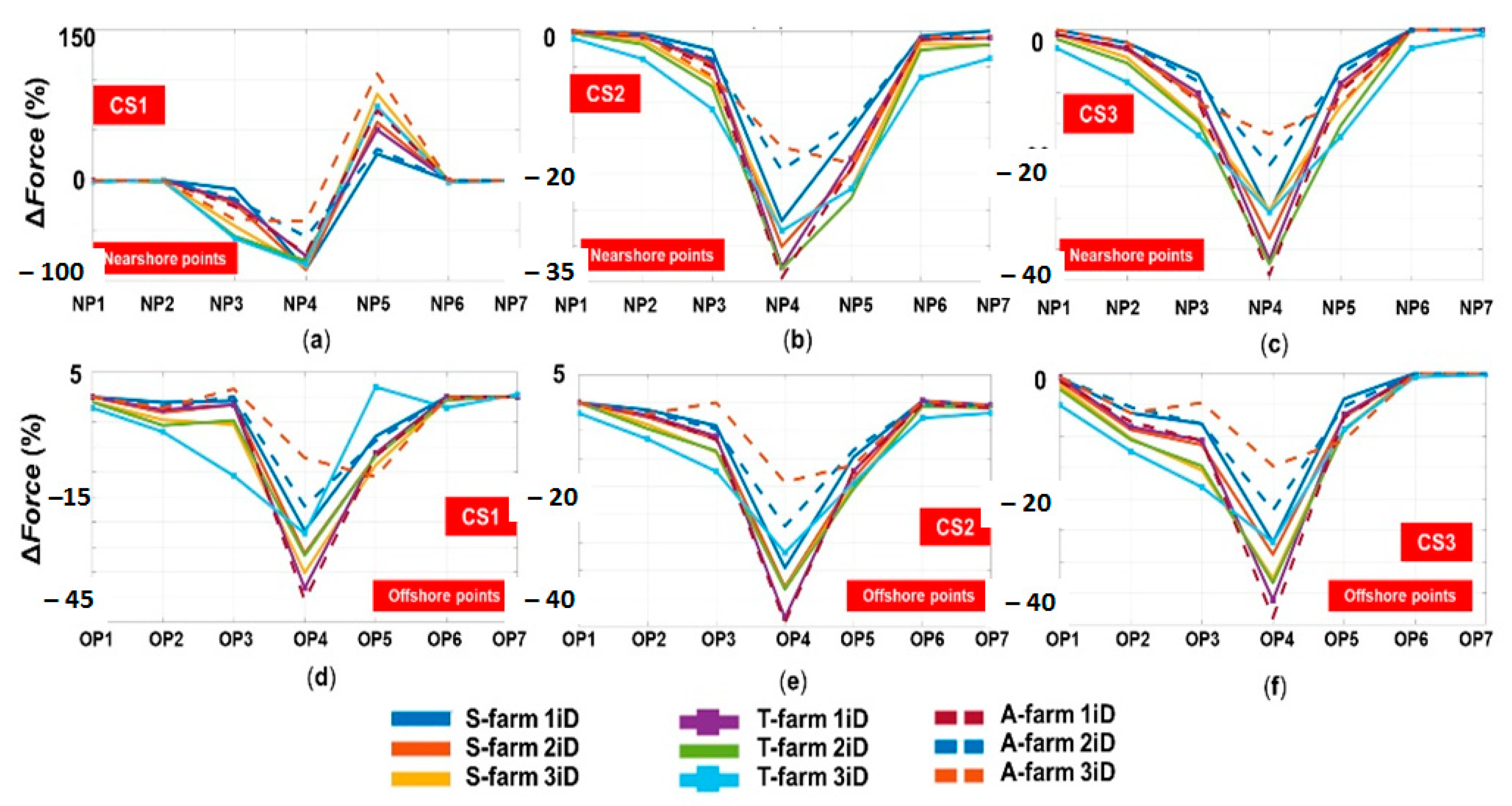
Figure 9 presents the variation of the wave forces by considering the presence of the wave farms. There was a big difference between the CS1–nearshore points where peaks of 90 or 110% (negative and positive, respectively) were noticed, while for the other scenarios and points, the peaks were negative and did not exceed 45%. For the nearshore points, a 1iD farm significantly reduced the forces for the point NP4 but increased the forces at NP5, especially if when considering a 3iD farm (+86% S-farm; +73%T-farm; +110% A-farm). On the extremity of the target area, the influence of the farms was negligible.
For scenario CS2, a 1iD farm provided a maximum force attenuation of 35% for the A-farm compared to 27% for the S-farm. Nevertheless, as we went from 1iD to 3iD, the A-farm was less efficient indicating for point NP4, a minimum value of 16% compared to 28% (S-farm and T-farm). From this perspective, the T-farm seemed to be the best solution, since the induced shielding effect covered a larger area including the points NP2 (3.9%) or NP6 (6.5%), respectively. As for scenario CS3, the distribution was almost symmetrical around the point NP4 with better performances observed: 37/39% –T-farm/A-farm (1iD); 37%–T-farm (2iD); 29%–S-farm/T-farm (3iD).
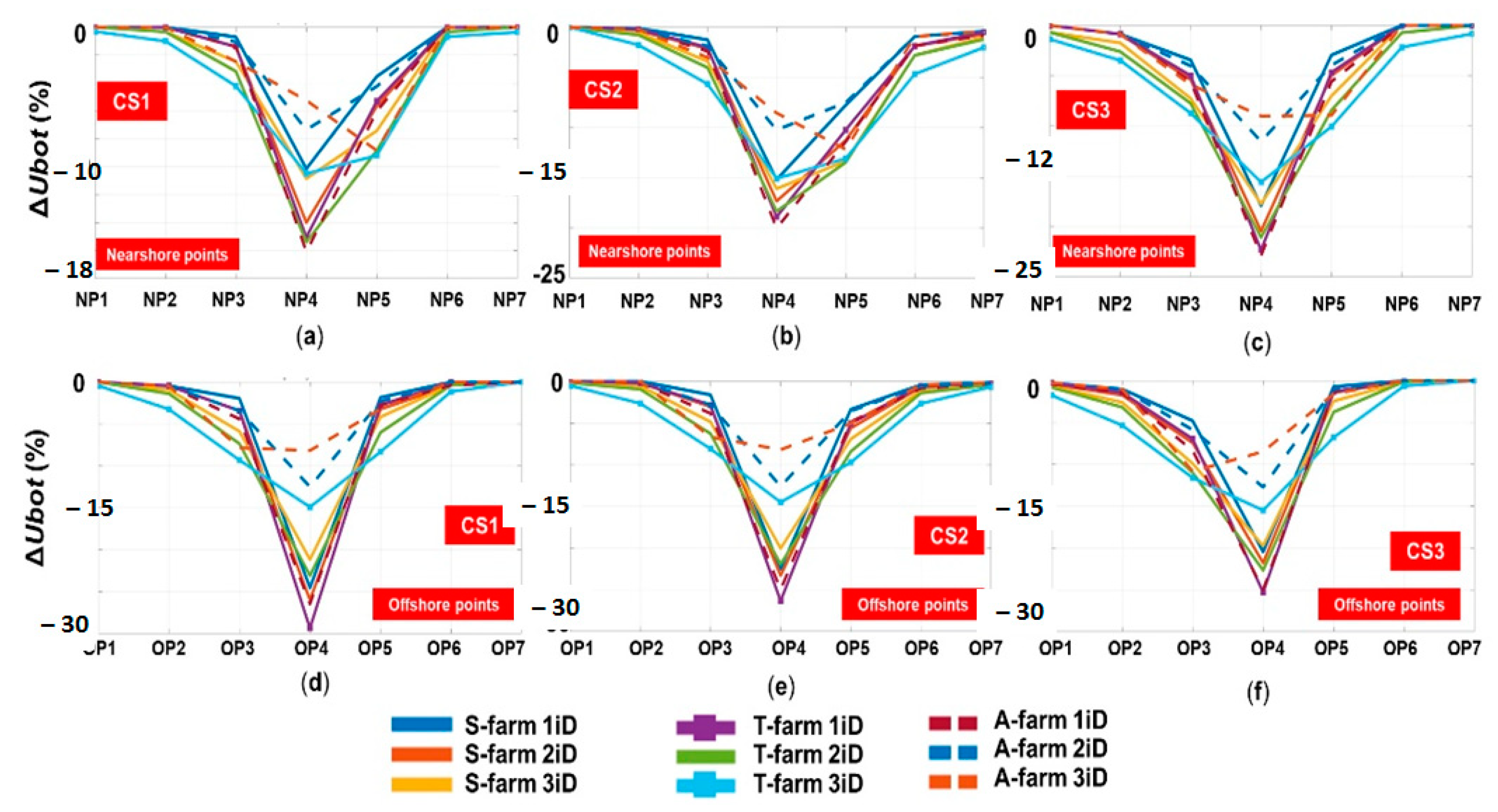
Figure 10 presents the variation of the parameter Ubot, the differences noticed being very similar to the ones corresponding to the Hs parameter (Figure 7).
The main reason for this situation was related to the fact that the variation of the orbital bottom velocity [55] is in the present work only related to the reduction in energy, which could be considered a limitation because the considered approach was not based on the frequency transmission coefficient. On the other hand, since the main objective of the present work was to provide a global picture of the down wave and shoreline impact of the marine energy farms, the approach considered could provide such a perspective. Furthermore, although the orbital velocity indicated, in general, a similar variation as the Hs parameter, by using the Hjulström curve [54] it was possible to establish some connections for the sediment circulation. Thus, the most important attenuations of the values were noticed in the central area, which meant that the wave balance could shift from erosion to sediment transport. By looking at the offshore points, in the case CS1, the erosion processes were dominant (Ubot in the range 1.47–2.75 m/s). For CS2 (offshore points), in the case of the large sediments (ex: cobbles and pebbles), the transport was bedload and deposition was representative (ex: minimum Ubot = 0.48 m/s). In this case, the presence of the wave farm increased the deposition processes. As for the nearshore points, the wave farm had little impact for the CS1 scenario, with more important changes noted for CS2 and CS3, where the suspension transport (ex: clay and silt) was accentuated.
4. Discussion
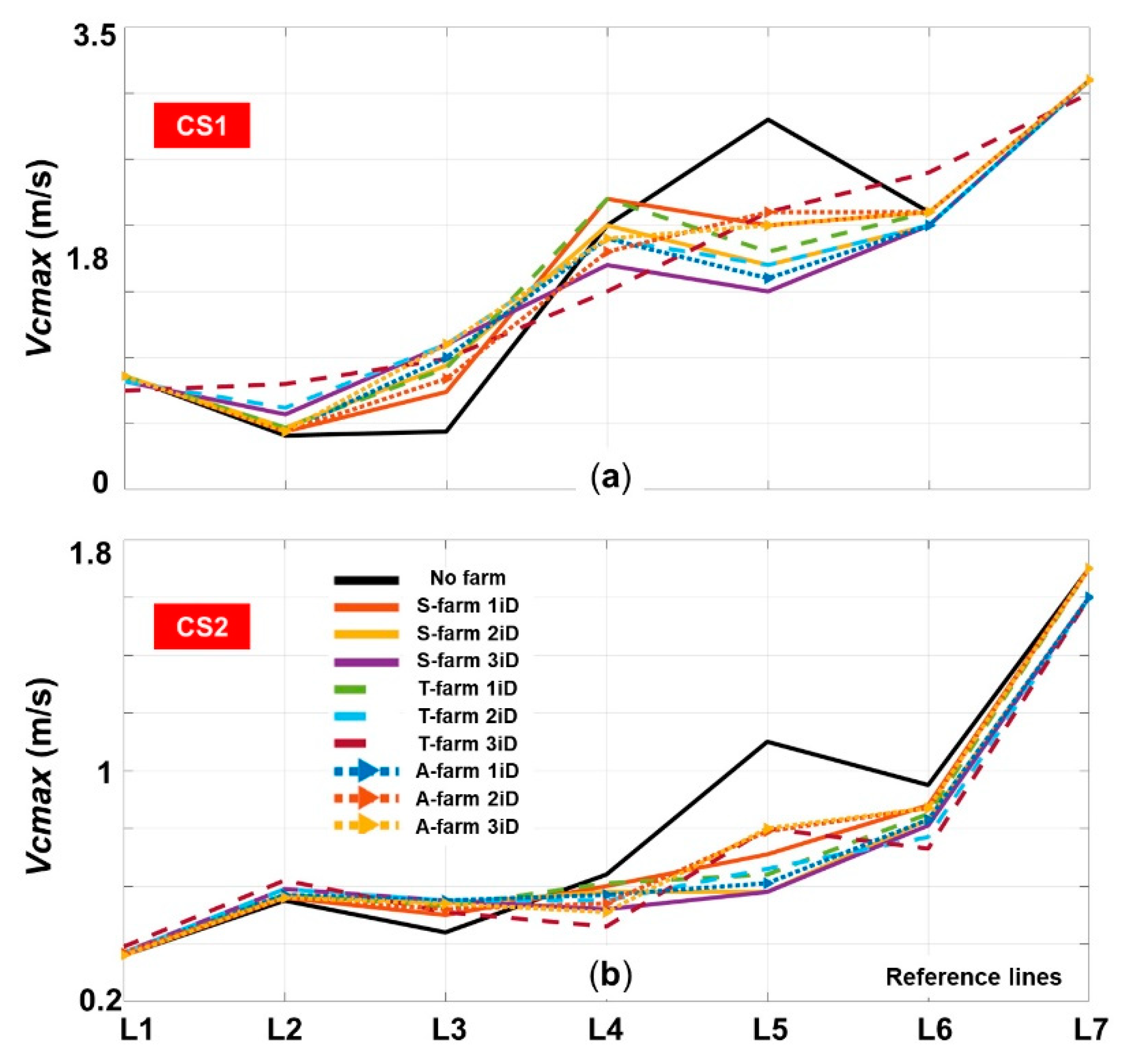
In this section, the evolution of the longshore currents will be investigated, by considering only two case studies. The first one is related to CS1 (extreme event), while from the other two (CS2 and CS3), only CS2 will be considered since the wave conditions are quite similar. Figure 11 presents the distribution of the maximum values of the current velocities along each reference line (from L1 to L7). Compared to the no farm scenario, it is possible to notice that the presence of a wave farm clearly shifts the evolution of the currents regardless of the case study considered. For scenario CS1 (Figure 11a), in the sector L1-L3, the presence of a wave farm will increase the current velocity from 0.41 m/s (no farm) to a maximum of 0.8 and 0.57 m/s for the T-farm and S-farm (3iD layout). For this line, the influence of the A-farm is minimal indicating a variation of 0.03 m/s. Higher values are noticed for the line L3, where all the farms indicate an increase of the velocity from 0.44 m/s (no farm) to a maximum of 1.1 m/s for S-farm/3iD, T-farm/2iD and A-farm/3iD, respectively. After the line L4, the current velocity jumps to a peak of 2.8 m/s (L5), followed by a value of 3.1 m/s (L7). For L5, a wave farm will reduce the velocity to 2.1 m/s (T-farm/3iD and A-farm/2iD) or to a minimum of 1.5 m/s (S-farm/3iD), respectively. As for CS2 (Figure 11b), the differences are smaller, being noticed an increase for line L3, from 0.44 m/s to a maximum value of 0.55 m/s (most of the configurations), while for L5 the velocity will decrease from 1.1 m/s (no farm) to a minimum of 0.58 m/s (S-farm/2iDand3iD). A lower impact on the line L5 corresponds to the T-farm/3iD and A-farm/2iD and 3iD that indicate values close to 0.8 m/s.
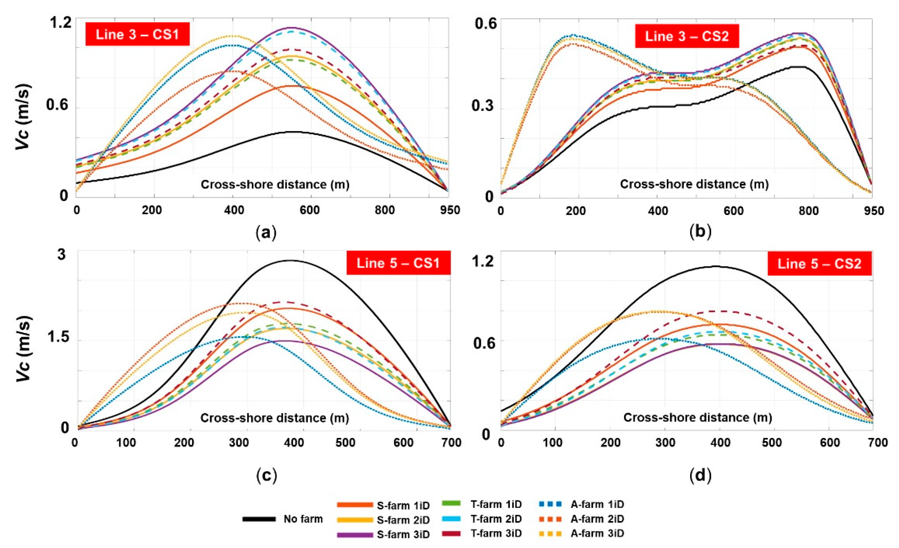
Figure 12 presents the profiles of the longshore currents for two reference lines (L3 and L5), that indicate a complex distribution of this parameter. For example in the case L3-CS1, it is noticed that each wave farm will increase the velocity, but also there is a tendency of the maximum peaks to move closer to the shoreline (by 200 m), as in the case of the A-farm layout.
In the case of Line 3–CS2, in general, the wave currents are defined by a higher slope when they are generated (at 950 m offshore), gradually decreasing as they go to the shore. The presence of an A-farm will reverse this process, the velocity gradually increasing offshore, and reaching a maximum peak at 200 m from the coastline after rapidly breaking down. For Line 5–CS1, the velocity has maximum values close to the shore, but this pattern is significantly changed by the A-farm that reaches higher values offshore (700 m from shore) and gradually attenuating to the shore.
5. Conclusions
During recent years, the signs of progress reported by the wave sector made plausible the idea of using wave energy farms as a soft engineering solution and, therefore, the present work is in line with similar researches, aiming to identify the expected coastal impact of some hypothetical wave farms by considering various layouts and device spacings [56,57]. The Obidos coastal environment is the target area that was considered for this investigation, in order to see how a wave project could influence the nearshore/offshore processes (in general) and how this can be used to protect the inlet of the Obidos lagoon (local). The selection of the Wave Dragon system was made by considering that this is one of the largest WECs from the market (project ongoing), it is designed to operate in the offshore area and is classified as a terminator system, which means that most of the incoming wave energy will be absorbed. Various wave farm configurations were considered (S-farm/T-farm/A-farm), by considering several distances between each WEC (1iD–2iD–3iD), with the mention that for some A-farms, configurations of only 5 systems were used, which could be considered a limitation of the present work.
By looking at the results related to the current velocities, we can say that the presence of a wave farm will have a big impact on the local conditions, and by reducing the wave heights, some other parameters will be influenced as well (ex: wave forces). The main problem with the Obidos lagoon (located between NP4 and NP5) is that during the wintertime the storm waves carry sediments in this area, which is finally trapped and creates problems for the local ecosystem. From the analysis of the CS1 scenario, it was found that the wave heights can be reduced by almost 16% (from 8 m–NP4) in the case of the 1iD or 2iD wave farms. It is important to mention that the main purpose of a wave farm is to generate electricity, but definitely, if there is interest to protect a particular coastal sector, the layout can be adjusted according to the season or some other particular requests. Since the wave farms were defined parallel to the coastline, the shielding effect induced is more visible in the central part of the target area, being mainly influenced by the wave direction. To anticipate this process, it is important to define some patterns that are considered significant for the coastal environment targeted, representing extreme and average wintertime conditions on one hand, and extreme summer conditions on the other hand. This was done by analyzing 27–years of combined ESA (satellite) and ERA5 (reanalysis) data. The summer average wave conditions were not considered, since they are characterized by relatively low energy.
As for the longshore currents, by modifying the breaking characteristics of the waves in the surf zone, some significant changes may be noticed in the case of the maximum velocity or current profiles. The natural tendency of the currents (no farm) is to increase from south to north, that for example in the case of CS1 can go from 0.41 (NP2) to 3.1 m/s (NP7). For the CS1 events, the presence of the wave farm will shift the currents pattern between L3 and L4 resulting in: (a) left side–an increase of the velocity of the current; (b) right side–local attenuation for L4 and L5. A similar pattern can be noticed for CS2, with a mention that the effects on the right side are more consistent. Finally, it has to be highlighted that there is significant wave energy potential in the Portuguese nearshore [58], but, on the other hand, there are also very active coastal processes [59]. From this perspective, the results of the present work show that a wave farm located close to Obidos lagoon, besides producing energy, has the potential to increase the efforts related to maritime spatial planning providing effective coastal protection.
Author Contributions
F.O. prepared the manuscript, including the set–up of the scenarios. L.R. processed the numerical data and contribute to the interpretation of the results. G.B.C. performed the literature review and processed the figures and tables. E.R. designed and supervised the present work. All authors have read and agreed to the published version of the manuscript.
Funding
This work was carried out in the framework of the research project DREAM (Dynamics of the Resources and technological Advance in harvesting Marine renewable energy), supported by the Romanian Executive Agency for Higher Education, Research, Development and Innovation Funding–UEFISCDI, grant number PNIII-P4-ID-PCE-2020-0008.
Institutional Review Board Statement
Not applicable.
Informed Consent Statement
Not applicable.
Data Availability Statement
The data used in this study are openly available in the public domain.
Acknowledgments
ERA5 data were generated using Copernicus Climate Change Service In-formation.
Conflicts of Interest
The authors declare no conflict of interest.
References
- Mentaschi, L.; Vousdoukas, M.I.; Pekel, J.-F.; Voukouvalas, E.; Feyen, L. Global Long-Term Observations of Coastal Erosion and Accretion. Sci. Rep. 2018, 8, 12876. [Google Scholar] [CrossRef] [Green Version]
- The World Factbook—Central Intelligence Agency. Available online: https://www.cia.gov/library/publications/the-world-factbook/geos/fr.html (accessed on 18 February 2018).
- Rusu, E.; Soares, C.G. Numerical Modelling to Estimate the Spatial Distribution of the Wave Energy in the Portuguese Nearshore. Renew. Energy 2009, 34, 1501–1516. [Google Scholar] [CrossRef]
- Rusu, L.; Soares, C.G. Impact of Assimilating Altimeter Data on Wave Predictions in the Western Iberian Coast. Ocean Model. 2015, 96, 126–135. [Google Scholar] [CrossRef]
- Specht, M.; Specht, C.; Lewicka, O.; Makar, A.; Burdziakowski, P.; Dąbrowski, P. Study on the Coastline Evolution in Sopot (2008–2018) Based on Landsat Satellite Imagery. J. Mar. Sci. Eng. 2020, 8, 464. [Google Scholar] [CrossRef]
- Quilfen, Y.; Yurovskaya, M.; Chapron, B.; Ardhuin, F. Storm Waves Focusing and Steepening in the Agulhas Current: Satellite Observations and Modeling. Remote Sens. Environ. 2018, 216, 561–571. [Google Scholar] [CrossRef] [Green Version]
- Pineau-Guillou, L.; Bouin, M.-N.; Ardhuin, F.; Lyard, F.; Bidlot, J.-R.; Chapron, B. Impact of Wave-Dependent Stress on Storm Surge Simulations in the North Sea: Ocean Model Evaluation against in Situ and Satellite Observations. Ocean Model. 2020, 154, 101694. [Google Scholar] [CrossRef]
- Stopa, J.E. Seasonality of Wind Speeds and Wave Heights from 30 years of Satellite Altimetry. Adv. Space Res. 2019. [Google Scholar] [CrossRef]
- Yaakob, O.; Hashim, F.E.; Omar, K.M.; Md Din, A.H.; Koh, K.K. Satellite-Based Wave Data and Wave Energy Resource Assessment for South China Sea. Renew. Energy 2016, 88, 359–371. [Google Scholar] [CrossRef]
- Mantas, V.M.; Pereira, A.J.S.C.; Neto, J.; Patrício, J.; Marques, J.C. Monitoring Estuarine Water Quality Using Satellite Imagery. The Mondego River Estuary (Portugal) as a Case Study. Ocean Coast. Manag. 2013, 72, 13–21. [Google Scholar] [CrossRef]
- Sá, C.; D’Alimonte, D.; Brito, A.C.; Kajiyama, T.; Mendes, C.R.; Vitorino, J.; Oliveira, P.B.; da Silva, J.C.B.; Brotas, V. Validation of Standard and Alternative Satellite Ocean-Color Chlorophyll Products off Western Iberia. Remote Sens. Environ. 2015, 168, 403–419. [Google Scholar] [CrossRef]
- Ruju, A.; Filipot, J.-F.; Bentamy, A.; Leckler, F. Spectral Wave Modelling of the Extreme 2013/2014 Winter Storms in the North-East Atlantic. Ocean Eng. 2020, 216, 108012. [Google Scholar] [CrossRef]
- Rusu, L.; Soares, C.G. Evaluation of a High-Resolution Wave Forecasting System for the Approaches to Ports. Ocean Eng. 2013, 58, 224–238. [Google Scholar] [CrossRef]
- Carvalho, D.; Rocha, A.; Gómez-Gesteira, M.; Silva Santos, C. Comparison of Reanalyzed, Analyzed, Satellite-Retrieved and NWP Modelled Winds with Buoy Data along the Iberian Peninsula Coast. Remote Sens. Environ. 2014, 152, 480–492. [Google Scholar] [CrossRef]
- Rusu, E.; Soares, C.G. Wave Energy Assessments in the Coastal Environment of Portugal Continental. In Proceedings of the Conference on Offshore Mechanics and Arctic Engineering—OMAE2008, Estoril, Portugal, 15–20 June 2008; Volume 6, pp. 761–772. [Google Scholar]
- Rusu, E. Evaluation of the Wave Energy Conversion Efficiency in Various Coastal Environments. Energies 2014, 7, 4002–4018. [Google Scholar] [CrossRef] [Green Version]
- Rusu, E. Numerical Modeling of the Wave Energy Propagation in the Iberian Nearshore. Energies 2018, 11, 980. [Google Scholar] [CrossRef] [Green Version]
- Do Carmo, J.S.A. The Changing Paradigm of Coastal Management: The Portuguese Case. Sci. Total Environ. 2019, 695, 133807. [Google Scholar] [CrossRef]
- Pranzini, E.; Williams, A.T. Coastal Erosion and Protection in Europe; Routledge: London, UK, 2013; ISBN 978-1-84971-339-9. [Google Scholar]
- Guillou, N.; Lavidas, G.; Chapalain, G. Wave Energy Resource Assessment for Exploitation—A Review. JMSE 2020, 8, 705. [Google Scholar] [CrossRef]
- Bergillos, R.J.; Rodriguez-Delgado, C.; Iglesias, G. Ocean Energy and Coastal Protection: A Novel Strategy for Coastal Management under Climate Change; Springer Briefs in Energy; Springer International Publishing: Cham, Switzerland, 2020; ISBN 978-3-030-31317-3. [Google Scholar]
- Onea, F.; Rusu, E. The Expected Shoreline Effect of a Marine Energy Farm Operating Close to Sardinia Island. Water 2019, 11, 2303. [Google Scholar] [CrossRef] [Green Version]
- Thomas, G. The Theory Behind the Conversion of Ocean Wave Energy: A Review. In Ocean Wave Energy; Cruz, J., Ed.; Green Energy and Technology (Virtual Series); Springer: Berlin/Heidelberg, Germany, 2008; pp. 41–91. ISBN 978-3-540-74894-6. [Google Scholar]
- Trueworthy, A.; DuPont, B. The Wave Energy Converter Design Process: Methods Applied in Industry and Shortcomings of Current Practices. JMSE 2020, 8, 932. [Google Scholar] [CrossRef]
- Norgaard, J.H.; Andersen, T.L.; Kofoed, J.P. Wave Dragon Wave Energy Converters Used as Coastal Protection; Takahashi, S., Kobayashi, N., Shimosako, K.I., Eds.; World Scientific Publ Co Pte Ltd.: Singapore, 2013; pp. 83–94. ISBN 978-981-4412-20-9. [Google Scholar]
- Cascajo, R.; García, E.; Quiles, E.; Correcher, A.; Morant, F. Integration of Marine Wave Energy Converters into Seaports: A Case Study in the Port of Valencia. Energies 2019, 12, 787. [Google Scholar] [CrossRef] [Green Version]
- Rusu, E.; Onea, F. Joint Evaluation of the Wave and Offshore Wind Energy Resources in the Developing Countries. Energies 2017, 10, 1866. [Google Scholar] [CrossRef] [Green Version]
- Onea, F.; Rusu, E. Sustainability of the Reanalysis Databases in Predicting the Wind and Wave Power along the European Coasts. Sustainability 2018, 10, 193. [Google Scholar] [CrossRef] [Green Version]
- Palha, A.; Mendes, L.; Fortes, C.J.; Brito-Melo, A.; Sarmento, A. The Impact of Wave Energy Farms in the Shoreline Wave Climate: Portuguese Pilot Zone Case Study Using Pelamis Energy Wave Devices. Renew. Energy 2010, 35, 62–77. [Google Scholar] [CrossRef]
- Rusu, E.; Soares, C.G. Coastal Impact Induced by a Pelamis Wave Farm Operating in the Portuguese Nearshore. Renew. Energy 2013, 58, 34–49. [Google Scholar] [CrossRef]
- A Setback for Wave Power Technology (Published 2009). Available online: https://www.nytimes.com/2009/03/16/business/global/16iht-renport.html (accessed on 20 November 2020).
- Bento, A.R.; Rusu, E.; Martinho, P.; Soares, C.G. Assessment of the Changes Induced by a Wave Energy Farm in the Nearshore Wave Conditions. Comput. Geosci. 2014, 71, 50–61. [Google Scholar] [CrossRef]
- Onea, F.; Rusu, E. The Expected Efficiency and Coastal Impact of a Hybrid Energy Farm Operating in the Portuguese Nearshore. Energy 2016, 97, 411–423. [Google Scholar] [CrossRef]
- Rusu, E.; Onea, F. Study on the Influence of the Distance to Shore for a Wave Energy Farm Operating in the Central Part of the Portuguese Nearshore. Energy Convers. Manag. 2016, 114, 209–223. [Google Scholar] [CrossRef]
- Bruneau, N.; Fortunato, A.B.; Dodet, G.; Freire, P.; Oliveira, A.; Bertin, X. Future Evolution of a Tidal Inlet Due to Changes in Wave Climate, Sea Level and Lagoon Morphology (Óbidos Lagoon, Portugal). Cont. Shelf Res. 2011, 31, 1915–1930. [Google Scholar] [CrossRef]
- Allard, J.; Bertin, X.; Chaumillon, E.; Pouget, F. Sand Spit Rhythmic Development: A Potential Record of Wave Climate Variations? Arçay Spit, Western Coast of France. Mar. Geol. 2008, 253, 107–131. [Google Scholar] [CrossRef]
- Oliveira, A.; Fortunato, A.B.; Rego, J.R.L. Effect of Morphological Changes on the Hydrodynamics and Flushing Properties of the Óbidos Lagoon (Portugal). Cont. Shelf Res. 2006, 26, 917–942. [Google Scholar] [CrossRef]
- Malhadas, M.S.; Silva, A.; Leitão, P.C.; Neves, R. Effect of the Bathymetric Changes on the Hydrodynamic and Residence Time in Óbidos Lagoon (Portugal). J. Coast. Res. 2009, 549–553. [Google Scholar]
- Piollé, J.-F.; Dodet, G.; Quilfen, Y. ESA Sea State Climate Change Initiative (Sea_State_cci): Global Remote Sensing Merged Multi-Mission Monthly Gridded Significant Wave Height, L4 Product, Version 1.1. Centre for Environmental Data Analysis, 2020. Available online: https://essd.copernicus.org/articles/12/1929/2020/ (accessed on 19 February 2021).
- Hersbach, H.; Bell, B.; Berrisford, P.; Hirahara, S.; Horányi, A.; Muñoz-Sabater, J.; Nicolas, J.; Peubey, C.; Radu, R.; Schepers, D.; et al. The ERA5 Global Reanalysis. Q. J. R. Meteorol. Soc. 2020, qj.3803. [Google Scholar] [CrossRef]
- The SWAN Team. SWAN Scientific and Technical Documentation, SWAN Cycle III Version 41.31A, Delft University of Technology. 2020. Available online: http://swanmodel.sourceforge.net/download/zip/swantech.pdf (accessed on 19 February 2021).
- Booij, N.; Ris, R.C.; Holthuijsen, L.H. A Third-Generation Wave Model for Coastal Regions: 1. Model Description and Validation. J. Geophys. Res. 1999, 104, 7649–7666. [Google Scholar] [CrossRef] [Green Version]
- Rusu, E.; Conley, D.; Ferreira-Coelho, E. A Hybrid Framework for Predicting Waves and Longshore Currents. J. Mar. Syst. 2008, 69, 59–73. [Google Scholar] [CrossRef]
- Rusu, E.; Soares, C.G. Validation of Two Wave and Nearshore Current Models. J. Waterw. Port. Coast. Ocean Eng. 2010, 136, 27–45. [Google Scholar] [CrossRef]
- Rusu, E.; Gonçalves, M.; Guedes Soares, C. Evaluation of the Wave Transformation in an Open Bay with Two Spectral Models. Ocean Eng. 2011, 38, 1763–1781. [Google Scholar] [CrossRef]
- Diaconu, S.; Rusu, E. The Environmental Impact of a Wave Dragon Array Operating in the Black Sea. Sci. World J. 2013, 498013. [Google Scholar] [CrossRef] [Green Version]
- Mendoza, E.; Silva, R.; Zanuttigh, B.; Angelelli, E.; Andersen, T.L.; Martinelli, L.; Norgaard, J.Q.H.; Ruol, P. Beach Response to Wave Energy Converter Farms Acting as Coastal Defence. Coast. Eng. 2014, 87, 97–111. [Google Scholar] [CrossRef]
- Smith, H.C.M.; Pearce, C.; Millar, D.L. Further Analysis of Change in Nearshore Wave Climate Due to an Offshore Wave Farm: An Enhanced Case Study for the Wave Hub Site. Renew. Energy 2012, 40, 51–64. [Google Scholar] [CrossRef]
- O’Dea, A.; Haller, M.C.; Özkan-Haller, H.T. The Impact of Wave Energy Converter Arrays on Wave-Induced Forcing in the Surf Zone. Ocean Eng. 2018, 161, 322–336. [Google Scholar] [CrossRef]
- López-Ruiz, A.; Bergillos, R.J.; Raffo-Caballero, J.M.; Ortega-Sánchez, M. Towards an Optimum Design of Wave Energy Converter Arrays through an Integrated Approach of Life Cycle Performance and Operational Capacity. Appl. Energy 2018, 209, 20–32. [Google Scholar] [CrossRef]
- The SWAN Team. SWAN User Manual, SWAN Cycle III Version 41.31A, Delft University of Technology. 2020. Available online: http://swanmodel.sourceforge.net/online_doc/swanuse/swanuse.html (accessed on 19 February 2021).
- IEC TS 62600-101:2015|IEC Webstore|Electricity, Water Management, Smart City, Rural Electrification, Marine Power. Available online: https://webstore.iec.ch/publication/22593 (accessed on 19 February 2021).
- Onea, F.; Rusu, L. A Long-Term Assessment of the Black Sea Wave Climate. Sustainability 2017, 9, 1875. [Google Scholar] [CrossRef] [Green Version]
- Woldegiorgis, B.T.; Van Griensven, A.; Bauwens, W. Explicit Incipient Motion of Cohesive and Non-cohesive Sediments Using Simple Hydraulics. Depos. Rec. 2018, 4, 78–89. [Google Scholar] [CrossRef] [Green Version]
- Shallow-Water Wave Theory-Coastal Wiki. Available online: http://www.coastalwiki.org/wiki/Shallow-water_wave_theory (accessed on 20 February 2021).
- Abanades, J.; Flor-Blanco, G.; Flor, G.; Iglesias, G. Dual Wave Farms for Energy Production and Coastal Protection. Ocean Coast. Manag. 2018, 160, 18–29. [Google Scholar] [CrossRef] [Green Version]
- Rijnsdorp, D.P.; Hansen, J.E.; Lowe, R.J. Understanding Coastal Impacts by Nearshore Wave Farms Using a Phase-Resolving Wave Model. Renew. Energy 2020, 150, 637–648. [Google Scholar] [CrossRef]
- Mota, P.; Pinto, J.P. Wave Energy Potential along the Western Portuguese Coast. Renew. Energy 2014, 71, 8–17. [Google Scholar] [CrossRef]
- Rusu, E.; Soares, G. Modeling waves in open coastal areas and harbors with phase resolving and phase averaged models. J. Coast. Res. 2013, 29, 1309–1325. [Google Scholar] [CrossRef]
Figure 1.
Map of the target area, Obidos nearshore in the Portuguese coastal environment.

Figure 2.
The computational domain considered for the SWAN numerical simulations, where: (a) bathymetric map including the positions of the nearshore points (NP) and offshore points (OF) and of the L—lines, respectively; (b) S—farm configuration; (c) T—farm configuration; (d) A—farm configuration where for the 2iD and 3iD case studies only 5 wave energy converters (denoted with *5 WECs) were considered.

Figure 3.
Wave statistics based on the ESA and ERA5 datasets, corresponding to the 27—year time interval (January 1992–December 2018), where: (a) Hs monthly evolution–average and extreme values as resulted from ESA and ERA5 datasets, respectively; (b) Tm monthly distribution—average and extreme values as provided by ERA5; (c,d) Mean wave directions and wave roses, as provided by ERA5 dataset.

Figure 4.
Hs field distribution in the presence of the wave farms considering the CS1 scenario, where: (a) S-farm; (b) T-farm; (c) A-farm. In the background, the wave vectors are represented, while the white dots correspond to the NP and OP points.
Figure 4.
Hs field distribution in the presence of the wave farms considering the CS1 scenario, where: (a) S-farm; (b) T-farm; (c) A-farm. In the background, the wave vectors are represented, while the white dots correspond to the NP and OP points.

Figure 5.
Hs field distribution in the presence of the wave farms considering the CS2 scenario, where: (a) S-farm; (b) T-farm; (c) A-farm. In the background, the wave vectors, are represented while the white dots correspond to the NP and OP points.
Figure 5.
Hs field distribution in the presence of the wave farms considering the CS2 scenario, where: (a) S-farm; (b) T-farm; (c) A-farm. In the background, the wave vectors, are represented while the white dots correspond to the NP and OP points.

Figure 6.
Hs field distribution in the presence of the wave farms considering the CS3 scenario, where: (a) S-farm; (b) T-farm; (c) A-farm. In the background, the wave vectors are represented, while the white dots correspond to the NP and OP points.
Figure 6.
Hs field distribution in the presence of the wave farms considering the CS3 scenario, where: (a) S-farm; (b) T-farm; (c) A-farm. In the background, the wave vectors are represented, while the white dots correspond to the NP and OP points.

Figure 7.
Variation of the Hs values (in %) in the presence of the wave farms in relationship with the no farm situation, where: (a–c) nearshore points–CS1, CS2 and CS3 scenarios; (d–f) offshore points–CS1, CS2 and CS3 scenarios.
Figure 7.
Variation of the Hs values (in %) in the presence of the wave farms in relationship with the no farm situation, where: (a–c) nearshore points–CS1, CS2 and CS3 scenarios; (d–f) offshore points–CS1, CS2 and CS3 scenarios.

Figure 8.
Variation of the Dir values (in %) in the presence of the wave farms in relation to the no farm situation, where: (a–c) nearshore points–CS1, CS2 and CS3 scenarios; (d–f) offshore points–CS1, CS2 and CS3 scenarios.
Figure 8.
Variation of the Dir values (in %) in the presence of the wave farms in relation to the no farm situation, where: (a–c) nearshore points–CS1, CS2 and CS3 scenarios; (d–f) offshore points–CS1, CS2 and CS3 scenarios.

Figure 9.
Variation of the wave force values (in %) in the presence of the wave farms in relation to the no farm situation, where: (a–c) nearshore points–CS1, CS2 and CS3 scenarios; (d–f) offshore points–CS1, CS2 and CS3 scenarios.
Figure 9.
Variation of the wave force values (in %) in the presence of the wave farms in relation to the no farm situation, where: (a–c) nearshore points–CS1, CS2 and CS3 scenarios; (d–f) offshore points–CS1, CS2 and CS3 scenarios.

Figure 10.
Variation of the Ubot values (in %) in the presence of the wave farms in relation to the no farm situation, where: (a–c) nearshore points–CS1, CS2 and CS3 scenarios; (d–f) offshore points–CS1, CS2 and CS3 scenarios.
Figure 10.
Variation of the Ubot values (in %) in the presence of the wave farms in relation to the no farm situation, where: (a–c) nearshore points–CS1, CS2 and CS3 scenarios; (d–f) offshore points–CS1, CS2 and CS3 scenarios.

Figure 11.
Evaluation of the wave farms impact on the maximum values of the nearshore currents (Vcmax–m/s), corresponding to the locations of the L-lines, where: (a) CS1 scenario; (b) CS2 scenario.
Figure 11.
Evaluation of the wave farms impact on the maximum values of the nearshore currents (Vcmax–m/s), corresponding to the locations of the L-lines, where: (a) CS1 scenario; (b) CS2 scenario.

Figure 12.
Nearshore currents profiles (m/s in the presence of the wave farms corresponding to the L-lines, where: (a,b) Line 3–CS1 and CS2 scenarios; (c,d) Line 5–CS1 and CS2 scenarios.
Figure 12.
Nearshore currents profiles (m/s in the presence of the wave farms corresponding to the L-lines, where: (a,b) Line 3–CS1 and CS2 scenarios; (c,d) Line 5–CS1 and CS2 scenarios.


Table 1.
Water depth (in m) corresponding to the nearshore and offshore points.
| Area | Reference Points | ||||||
|---|---|---|---|---|---|---|---|
| 1 | 2 | 3 | 4 | 5 | 6 | 7 | |
| Nearshore | 10.02 | 14.06 | 16.09 | 13.47 | 16.71 | 12.25 | 12.87 |
| Offshore | 24.07 | 26.07 | 27.61 | 25.41 | 24.88 | 19.45 | 18.27 |
Table 2.
The SWAN model configuration corresponding to the Obidos computational domain.
| Wave | Wind | Tide | Crt | Gen | Wcap | Quad | Triad | Diff | Bfric | Setup | Br | |
|---|---|---|---|---|---|---|---|---|---|---|---|---|
| x | x | – | x | x | x | x | x | x | x | x | x | |
| Input/Process | Coordinates | ∆x × ∆y (m) | ∆θ (°) | Mod | nθ | nf | ngx × ngy = np | |||||
| Cartesian | 50 × 50 | 5 | Stat/BSBT | 36 | 34 | 362 × 305 = 110,410 | ||||||
Table 3.
Offshore sea states considered for the Obidos site in the Portuguese nearshore, based on ESA and ERA5 datasets.
Table 3.
Offshore sea states considered for the Obidos site in the Portuguese nearshore, based on ESA and ERA5 datasets.
| Month | ESA Dataset | ERA5 Dataset | ERA5 Dataset |
|---|---|---|---|
| Hs (m) | Tm (s) | Dir (°) | |
| CS1–February (extreme) | 9 | 16.8 | 304 |
| CS2–January (average) | 3.1 | 10.9 | 298 |
| CS3–July (extreme) | 3.7 | 12.2 | 324 |
Table 4.
Hs values (m) corresponding to the nearshore and offshore reference points for the case studies considered–without the wave farm.
Table 4.
Hs values (m) corresponding to the nearshore and offshore reference points for the case studies considered–without the wave farm.
| Wave Conditions | Reference Points | ||||||
|---|---|---|---|---|---|---|---|
| 1 | 2 | 3 | 4 | 5 | 6 | 7 | |
| CS1–offshore | 8.29 | 8.36 | 8.26 | 8.01 | 8.14 | 8.32 | 8.42 |
| CS2–offshore | 2.82 | 2.8 | 2.79 | 2.74 | 2.73 | 2.87 | 2.83 |
| CS3–offshore | 3.3 | 3.32 | 3.27 | 3.22 | 3.2 | 3.51 | 3.64 |
| CS1–nearshore | 6.7 | 7.72 | 7.99 | 7.28 | 8.15 | 6.99 | 6.73 |
| CS2–nearshore | 2.81 | 2.79 | 2.74 | 2.68 | 2.76 | 2.97 | 2.84 |
| CS3–nearshore | 3.38 | 3.37 | 3.31 | 3.17 | 3.28 | 3.65 | 3.31 |
Table 5.
Mean wave direction (Dir) values (°) corresponding to the nearshore and offshore reference points for the case studies considered–without the wave farm.
Table 5.
Mean wave direction (Dir) values (°) corresponding to the nearshore and offshore reference points for the case studies considered–without the wave farm.
| Wave Conditions | Reference Points | ||||||
|---|---|---|---|---|---|---|---|
| 1 | 2 | 3 | 4 | 5 | 6 | 7 | |
| CS1–offshore | 310 | 310 | 309 | 307 | 306 | 305 | 308 |
| CS2–offshore | 303 | 303 | 303 | 302 | 300 | 301 | 303 |
| CS3–offshore | 322 | 321 | 320 | 318 | 316 | 319 | 321 |
| CS1–nearshore | 318 | 314 | 312 | 308 | 304 | 305 | 300 |
| CS2–nearshore | 310 | 308 | 306 | 305 | 300 | 298 | 293 |
| CS3–nearshore | 322 | 321 | 320 | 316 | 312 | 313 | 307 |
Table 6.
Wave forces values (N/m2) corresponding to the nearshore and offshore reference points for the case studies considered—without the wave farm.
Table 6.
Wave forces values (N/m2) corresponding to the nearshore and offshore reference points for the case studies considered—without the wave farm.
| Wave Conditions | Reference Points | ||||||
|---|---|---|---|---|---|---|---|
| 1 | 2 | 3 | 4 | 5 | 6 | 7 | |
| CS1–offshore | 10.2 | 5.45 | 12.7 | 11.5 | 5.58 | 46.2 | 5.95 |
| CS2–offshore | 1.05 | 0.54 | 0.85 | 1.04 | 0.64 | 2.89 | 2.16 |
| CS3–offshore | 1.58 | 0.87 | 1.49 | 1.56 | 0.83 | 4.98 | 3.82 |
| CS1–nearshore | 70.9 | 31.4 | 11.1 | 31.8 | 7.86 | 91.5 | 85.9 |
| CS2–nearshore | 9.46 | 5.36 | 4.12 | 7.76 | 3.08 | 9.82 | 10.4 |
| CS3–nearshore | 13.8 | 8.09 | 6.42 | 11.3 | 4.56 | 16.8 | 13.3 |
Table 7.
The orbital velocity (Ubot) values (m/s) corresponding to the nearshore and offshore reference points for the case studies considered—without the wave farm.
Table 7.
The orbital velocity (Ubot) values (m/s) corresponding to the nearshore and offshore reference points for the case studies considered—without the wave farm.
| Wave Conditions | Reference Points | ||||||
|---|---|---|---|---|---|---|---|
| 1 | 2 | 3 | 4 | 5 | 6 | 7 | |
| CS1–offshore | 2.25 | 2.15 | 2.04 | 2.08 | 2.16 | 2.61 | 2.75 |
| CS2–offshore | 0.57 | 0.52 | 0.49 | 0.52 | 0.53 | 0.71 | 0.73 |
| CS3–offshore | 0.73 | 0.69 | 0.64 | 0.68 | 0.69 | 0.94 | 1.03 |
| CS1–nearshore | 3.17 | 2.98 | 2.84 | 2.86 | 2.83 | 2.92 | 2.74 |
| CS2–nearshore | 1.17 | 0.9 | 0.79 | 0.88 | 0.77 | 1.07 | 0.98 |
| CS3–nearshore | 1.46 | 1.15 | 1.02 | 1.11 | 0.98 | 1.38 | 1.21 |
Publisher’s Note: MDPI stays neutral with regard to jurisdictional claims in published maps and institutional affiliations. |
© 2021 by the authors. Licensee MDPI, Basel, Switzerland. This article is an open access article distributed under the terms and conditions of the Creative Commons Attribution (CC BY) license (http://creativecommons.org/licenses/by/4.0/).
Share and Cite
MDPI and ACS Style
Onea, F.; Rusu, L.; Carp, G.B.; Rusu, E. Wave Farms Impact on the Coastal Processes—A Case Study Area in the Portuguese Nearshore. J. Mar. Sci. Eng. 2021, 9, 262. https://doi.org/10.3390/jmse9030262
AMA Style
Onea F, Rusu L, Carp GB, Rusu E. Wave Farms Impact on the Coastal Processes—A Case Study Area in the Portuguese Nearshore. Journal of Marine Science and Engineering. 2021; 9(3):262. https://doi.org/10.3390/jmse9030262
Chicago/Turabian StyleOnea, Florin, Liliana Rusu, Gabriel Bogdan Carp, and Eugen Rusu. 2021. "Wave Farms Impact on the Coastal Processes—A Case Study Area in the Portuguese Nearshore" Journal of Marine Science and Engineering 9, no. 3: 262. https://doi.org/10.3390/jmse9030262
Note that from the first issue of 2016, this journal uses article numbers instead of page numbers. See further details here.