An Extended VIKOR-Based Approach for Pumped Hydro Energy Storage Plant Site Selection with Heterogeneous Information

1
School of Economics and Management, North China Electric Power University, Beijing 102206, China
2
Beijing Key Laboratory of New Energy and Low-Carbon Development, North China Electric Power University, Changping, Beijing 102206, China
*
Author to whom correspondence should be addressed.
Information 2017, 8(3), 106; https://doi.org/10.3390/info8030106
Submission received: 28 July 2017
/
Revised: 23 August 2017
/
Accepted: 26 August 2017
/
Published: 30 August 2017
(This article belongs to the Section Information Theory and Methodology)
Abstract
:The selection of a desirable site for constructing a pumped hydro energy storage plant (PHESP) plays a vital important role in the whole life cycle. However, little research has been done on the site selection of PHESP, which affects the rapid development of PHESP. Therefore, this paper aims to select the most ideal PHESP site from numerous candidate alternatives using the multi-criteria decision-making (MCDM) technique. Firstly, a comprehensive evaluation criteria system is established for the first time. Then, considering quantitative and qualitative criteria coexist in this system, multiple types of representations, including crisp numerical values (CNVs), triangular intuitionistic fuzzy numbers (TIFNs), and 2-dimension uncertain linguistic variables (2DULVs), are employed to deal with heterogeneous criteria information. To determine the weight of criteria and fully take the preference of the decision makers (DMs) into account, the analytic hierarchy process (AHP) method is applied for criteria weighting. After that, an extended Vlsekriterijumska Optimizacija I Kompromisno Resenje (VIKOR) method is utilized to provide compromise solutions for the PHESP site considering such heterogeneous information. At last, the proposed model is then applied in a case study of Zhejiang province, China to illustrate its practicality and efficiency. The result shows the Changlongshan should be selected as the optimal PHESP.
1. Introduction
In recent years, with the increasingly serious environmental pollution and aggravation of the global energy crisis, developing renewable energy vigorously has become an inevitable choice of mankind. Wind energy and solar energy, as reliable and promising forms of renewable energy, have been developing swiftly worldwide. It is noteworthy that, in 2016, China’s total installed capacity of wind power and solar power both ranked first in the world. However, at the same time, the phenomenon of power curtailment is becoming increasingly prominent since wind and solar energy are characterized by volatility and intermittency [1]. This kind of phenomenon has brought humans huge economic loss and restricted the development of renewable energy. One of the main causes of this phenomenon is that the current peak shaving capacity of the power system is seriously poor. The current power source structure in China is unreasonable, and the thermal power as the main structure of the power source accounts for 71.1%. However, the load response of thermal power is slow, resulting in the shortage of its peak capacity.
Energy storage systems are one of the possible solutions for mitigating the effects of intermittent renewable resources [2]. Among all energy storage technologies, pumped hydro energy storage (PHES) technology is the most widely used. The share of various storage technologies in the global electricity storage system is shown in Figure 1. Although a lot of forms of energy storage technology have been developed, the PHES technology accounted for the energy storage of absolute dominance. PHES is now one of the most mature and cost-effective technologies since water lifting devices have been invented, used, and improved by humans, for thousands of years [1]. This technique uses electricity produced by other power stations to pump water up to the upper reservoir when the energy demand is low, and release the water back down to the lower reservoir to generate electricity when the energy demand is high [3]. Thanks to the fast response ability of PHESPs, a huge push to build them will ensure that electricity production matches demands at all times.
In June 2017, the installed capacity of PHESPs in China reached 27.73 million kW, surpassed Japan, and became the biggest capacity of PHESP in the world. But despite all that, the proportion of pumped storage in electric power systems in China is less than 2%. Thus, lately, the “13th Five-Year Plan for Electric Power Development” released by the National Energy Administration (NEA) made it clear that the installed capacity of the new pumped hydro energy storage plant must arrive at 60 million kWh by 2020. There is no doubt that the PHES industry is in an important period of strategic opportunities for accelerated development.
In recent years, the existing literature on various aspects of PHESP has become much more enriched. Rogeau et al. [1] proposed a generic method able to evaluate the potential of small-PHESP over a large geographical zone. Gimeno-Gutierrez and Lacal-Arantegui [4] assessed a PHESP potential based on two existing reservoirs in Europe by developing and applying a GIS-based software model. Petrakopoulou et al. [5] conducted a simulation and analysis of a stand-alone solar-wind and PHESP in the Aegean Sea. Pérez-Díaz et al. [6] aimed at assessing the contribution of pumped-hydro energy storage to reduce the scheduling costs of hydrothermal power systems with high wind penetration, which may yield unrealistic results. Pérez-Díaz and Chazarra [7] reviewed the current trends in the PHESP operation, and presented the main challenges faced by PHESP operators. Yang and Jackson [8] analyzed the opportunities and barriers to PHESP in the United States. By contrast, there has been relatively little research on the site selection of PHESP. For example, Lu and Wang [9] provided promising locations of the PHESPs through Geographic Information Science (GIS) analyses. Kucukali [10] found the most suitable existing hydropower reservoirs for the development of PHS by using the multi-criteria scoring technique. Also, Connolly et al. [11] developed a computer program to locate potential sites for pumped hydroelectric energy storage. However, in the entire life cycle of the renewable energy plant, the site selection is important and determines the sustainable development ability and socio-economic values of the power plant [12]. At the meantime, identifying suitable sites for PHESP is a complex task since many potential site alternatives are feasible. Thus, by all appearances, the site selection of PHESP is a valuable research issue.
A number of conflicting criteria need to be taken into account simultaneously in the process of PHESP site selection. So, the site selection of PHESP can be defined as a MCDM problem. MCDM is a well-known branch of decision-making, which aims to find the most suitable solutions from a set of alternatives under multiple criteria conditions [13]. Nevertheless, existing methods for solving MCDM problems that are not applicable for the site selection of PHESP, which are mainly reflected in the loss of information. In detail, the complexity of PHESP site selection is much higher than other MCDM problems since it is very strict with topography and geomorphology. Also, many data are impossible to obtain, and they are also inaccurate. So, in such a complex decision-making environment, the best way to give a reasonable representation of the criteria value and preserve the integrity of the original decision information is very difficult to establish.
Therefore, this paper tries to select the optimal PHESP site and handle the problem of information loss in this process. Firstly, an evaluation criteria system of PHESP site selection is established. Then, according to the properties of the identified criteria, we divide them into three categories: quantitative criteria that can be measured accurately, quantitative criteria that cannot be measured accurately, and qualitative criteria. The values of the three categories are represented by CNVs, TIFNs, and 2DULVs, respectively. In this way, the criteria values with different natures can be better described. Furthermore, based on Hamming distance, the VIKOR method is proposed to rank the PHESP sites. This method is particularly useful for those problems for which the values of the alternatives are not represented by the same units, since there is no need to translate different forms of decision information. The innovations of this paper are as follows: (1) a comprehensive evaluation criteria system is established; (2) an extended VIKOR-based MCDM approach with heterogeneous criteria values comprising CNVs, TIFNs, and 2DULVs is proposed.
2. Literature Review
The values of the criteria involved in site selection not only contain objective quantitative statistical data, but include some subjective judgment data given by DMs with their knowledge and experience. Thus, using a single form of decision information makes it difficult to meet the requirement of site selection decision-making. Most scholars have recognized this problem, and utilized different forms of decision information to represent criteria of different characteristics. Among various information forms, numerical numbers, interval numbers, linguistic variables, and fuzzy numbers are the most commonly used forms. Wu and Chen [14] used CNVs and linguistic variables (LVs) to describe the values of criteria involved in waste-to-energy plant site selection. Wu and Geng [15] applied CNVs and LVs to model the values of criteria involved in solar thermal power plant site selection. Later, both the two studies converted the CNVs into the LVs for convenience of calculation. Sánchez-Lozano et al. [16] utilized CNVs, LVs, and triangular fuzzy numbers (TFNs) to represent the values of criteria involved in onshore wind farm site selection, and then, the CNVs and LVs were both converted into the TIFNs. Wu and Zhang [17] utilized CNVs and LVs to represent the values of criteria involved in offshore wind power station site selection, and transformed both the CNVs and the LVs into intuitionistic fuzzy numbers (IFNs). Also, Wu et al. [18] used CNVs and IFNs in the process of wind farm project plan selection, and then, the CNVs were transformed into the IFNs. In addition, some extended forms of LVs have been also applied, such as 2-tuple linguistic variables. CNVs and 2-tuple linguistic variables are used in the process of low-speed wind farm site selection; after that, both of them are transformed into 2-tuple linguistic variables [19].
The contribution of the above literatures in the field of site selection is understandable. However, there are some problems that have not been well solved. Firstly, for qualitative criteria, their values are generally assessed by DMs with their knowledge and experience. Due to the complexity of PHESP site selection, some DMs may not be very confident about their assessment. In other words, the assessments given by DMs are not very reliable in some cases. However, the current forms of decision information, such as the 2-tuple linguistic variables, have not taken this into account. Secondly, the different forms of decision information in the above studies have been unified into one kind of decision information. Nevertheless, information loss will inevitably occur in such a unification process.
As for the first question, it is necessary to introduce the 2DUIVs. The 2-dimension linguistic variables (2DLVs) were proposed by Zhu et al. [20] in 2009 and include two common linguistic labels to precisely assess alternatives with linguistic information. One dimension is used for describing the evaluation result of alternatives provided by the DM, and the other is used for describing the self-assessment of the DM on the reliability of the given evaluation result. However, due to time pressure, and lack of knowledge and information processing capabilities, the evaluation information provided by DMs may not match any of the original linguistic phrase, and it may be between two linguistic phrases [21]. For this reason, Liu and Zhang [22] extended 2DIVs to 2DULVs, and developed a method to deal with the MCDM problem in which the criteria values take the form of 2-dimension uncertain linguistic information. Naturally, the 2DUIVs spread in the MCDM field [23,24,25]. Thus, introducing the 2DULVs to represent the values of qualitative criteria involved in PHESP site selection is a meaningful work, which reflects more accurately the assessment of DM on alternatives and decreases the information loss.
To solve the second problem, some distance-based techniques play an important role. Among them, the Technique for Order Preference by Similarity to Ideal Solution (TOPSIS) approach and the VIKOR approach are the most commonly used techniques. They are particularly useful for those problems for which the values of the criteria are not represented by the same forms. The core idea of them is to calculate the relative gaps between each alternative and the optimal alternative by means of distance formula associated with hybrid criteria. In view of this, Wu and Xu [26] studied the site selection problem of the tidal power plant with the criteria value as numerical numbers, interval numbers, and random numbers; then, a rank method based on TOPSIS was proposed. Matsui et al. [27] presented a modified VIKOR method based on numerical numbers, fuzzy numbers, interval numbers, and linguistic variables. Sun and Liu [28] handled with numerical numbers, fuzzy numbers, interval numbers, and linguistic variables simultaneously to evaluate the candidate power system restoration alternatives based on an extended VIKOR method. However, it have been proved that the TOPSIS approach cannot reflect the closeness of the alternatives to positive and negative ideal solutions [29]. In contrast, the VIKOR method can overcome the shortcomings of the TOPSIS approach; in addition, it considers a maximum group utility and a minimum of individual regret simultaneously and takes into account the subjective preference of DMs [30,31]. In recent years, the research on the extension and application of VIKOR methods has attracted the attention of some scholars. For example, Mousavi and Jolai [32] used a stochastic VIKOR to evaluate and rank probability distributions for each alternative. Liu and You [33] used a fuzzy VIKOR for failure mode and effects analysis; triangular fuzzy numbers are preferred to express linguistic evaluations. Mokhtarian and Sadi-Nezhad [34] used fuzzy VIKOR on interval-valued fuzzy numbers for facility site selection problems. You and You [35] used the linguistic VIKOR method for supplier selection; the attributes are expressed with 2-tuple linguistic variables. As can be seen from the above, the VIKOR method has been successfully applied in various fields. Therefore, this work tries to adopt the VIKOR method to rank candidate PHESP alternatives.
3. Evaluation Criteria System of PHESP Site Selection
The evaluation criteria are important for the establishment of the criteria system for PHESP site selection. To do this, firstly, a lot of criteria were collected initially in light of the academic literature and feasibility research reports. Then, a total of seven experts whose academic backgrounds are hydrology, geological, engineering, renewable energy, and social, economic, and environmental fields were invited and an expert meeting was organized. In this meeting, the list of initial criteria were distributed to the experts and each expert issued his/her judgement. After several rounds of discussion, experts reached an agreement; the final criteria and sub-criteria of PHESP site selection are established and listed in Table 1. The first criteria reflect the impacts of various local conditions on the potential PHESP; the last three criteria are the impacts induced by the PHESP after completion. The analysis of these criteria and sub-criteria is given in Appendix A.
PHESP site selection involves selecting the optimal one through comparing the alternatives against a series of qualitative and quantitative criteria. The sub-criteria values can be divided into three types: quantitative criteria can be measured accurately, quantitative criteria cannot be measured accurately, and qualitative criteria. (1) The first type of sub-criteria include C11, C12, C13, C14, and C15. The value of such sub-criteria can be measured definitely and expressed by CNVs; (2) the second type of sub-criteria include C31, C32, C33, C34, C41, C42, and C43. Due to the restriction of measuring and forecasting technology, the sub-values of criteria C11, C13, and C31 is expressed by TIFNs; (3) the last type of sub-criteria include C21, C22, and C23. It’s difficult to quantify their values by measurement methods, so it’s common to invite experts to score those sub-criteria with respect to the alternatives. Because of the inherent vagueness of human thinking, DMs express their preferences or assessments by using 2DUIVs.
4. Preliminaries
4.1. Triangular Intuitionistic Fuzzy Number
In this section, we review the definition and operation rules of TIFNs and give the Hamming distance for TIFNs.
4.1.1. Definition of Triangular Intuitionistic Fuzzy Number
Definition 1 [36].
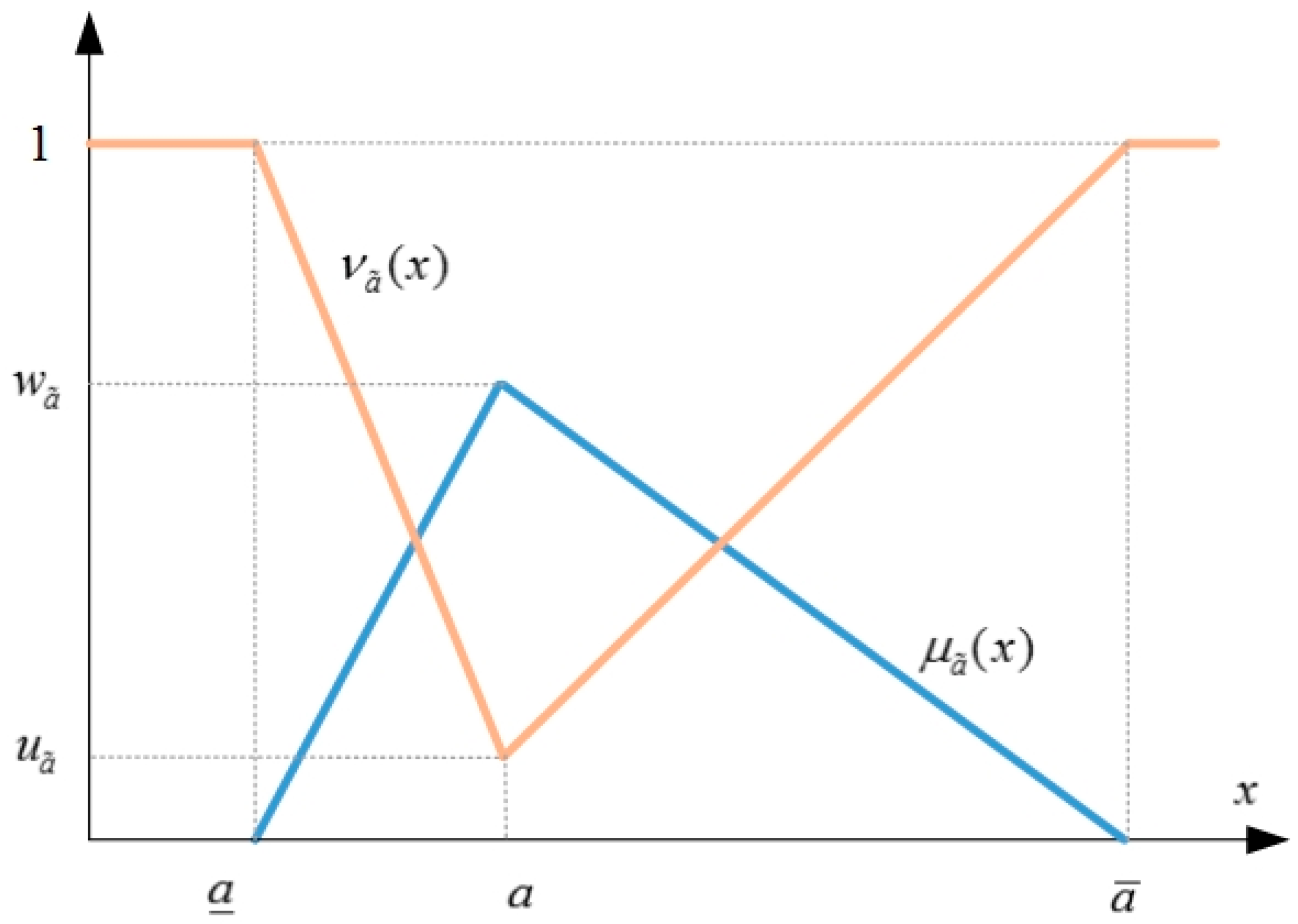
A TIFN is a special IFS on the real number set , whose membership function and non-membership function are defined as follows:
respectively, depicted as in Figure 2; the values and represent the maximum membership degree and the minimum non-membership degree such that they satisfy the conditions: and . Let is called an intuitionistic fuzzy index of the TIFN , which reflects hesitancy degree of the element to .
4.1.2. Operation Rules of Triangular Intuitionistic Fuzzy Number
Definition 2 [36].
Let and be two TIFNs and be a real number. Then the arithmetical operations for TIFNs are defined as follows:
- (1)
- (2)
where the symbols “” and “” mean min and max operators, respectively.
4.1.3. Distance between Two Triangular Intuitionistic Fuzzy Numbers
Definition 3 [37].
Let and be two TIFNs. The Hamming distance between and is defined as follows:
4.2. 2-Dimension Uncertain Linguistic Variable
4.2.1. Definition of 2-Dimension Uncertain Linguistic Variable
Definition 4 [38].
Let , where is I class uncertain linguistic information, which represents decision maker’s judgment to an evaluated object, and are the elements from the predefined linguistic assessment set , while is II class uncertain linguistic information, which represents the subjective evaluation on the reliability of their given results, and are the elements from the predefined linguistic assessment set , then is called the 2-dimension uncertain linguistic variable.
4.2.2. Operational Rules of 2-Dimension Uncertain Linguistic Variable
- (1)
- (2)
4.2.3. Distance between Two 2-Dimension Uncertain Linguistic Variables
Definition 6 [38].
Let and be two 2DULVs, the Hamming distance of and is defined as follows:
4.3. VIKOR Method
The VIKOR method, proposed by Opricovic [39], would be an effective tool for the MCDM process when the DM is unable to take a decision or doesn’t know to express their preferences at the beginning stage [40]. This method generates a multi-criteria ranking index, which is developed from an aggregating function representing ‘‘closeness” to “ideal” solution. The ranking index is developed from metric, an aggregating function in compromise programming. The VIKOR method uses a linear normalization method to eliminate the units of criteria and determines a compromise solution, which represents maximum “group utility” and a minimum individual regret for the “majority” and “opponent”, respectively [31].
Allow that there are alternatives generated for any complex problem of decision making. As an alternative, ; is the performance value of -th criterion function. The metric, which was used for starting the development of the ranking measure of the VIKOR method, is as follows:
and are used to formulate the ranking measures and in the VIKOR method, respectively. The maximum group utility (“majority rule”) and minimum individual regret of the “opponent” is calculated by min and min , respectively.
5. An Extended, VIKOR-Based MCDM Approach with Heterogeneous Information
Consider a MCDM problem with three types of values: CNVs, TIFNs, and 2DULVs. The alternatives set is , and the criteria set is . Among it, the criteria set with CNVs is , TIFNs is , and 2DULVs is . A CNV is expressed as , a TIFN is expressed as , and a 2DULV is expressed as . The pre-defined linguistic assessment sets are and .
Step 1: Normalize decision matrix.
This step performs the normalization process of the decision matrix. The data in the decision matrix are normalized to unify different measurement scales. The normalized matrix , composed by a mixture of CNVs, TIFNs, and 2DULVs, can be expressed as follows:
The normalized values for benefit- and cost-related criteria are calculated using the following equations:
Step 2: Determine PIS and NIS, respectively:
where is PIS and is NIS; denote the set of CNVs, TIFNs and 2DULVs, respectively.
Step 3: Calculate the separation measures
The calculation of the separation of each alternative with respect to the PIS and NIS, respectively, based on the Hamming distance. The distance between two CNVs is an absolute value of difference, and the distance between two TIFNs and 2DULVs is calculated according to Formulas (1) and (2).
Step 4: Calculate criteria weight
Reasonable weights for decision criteria may be obtained by many techniques, one of which is the AHP [41]. It utilizes pair-wise comparisons for a set of criteria to judge the relative importance between one attribute and another. In this context, the fundamental “1–9 scale” defined by Saaty is employed for DMs to evaluate the priority score. The judgment matrix is constructed as follows:
where the element indicates representation of relative importance between criteria and .
Step 5: Calculate the values of , , and by the relations:
where is the group utility of alternative; is the individual regret of the worst index of ; is the weight of majority criteria; and is the weight of individual regret.
Step 6: Rank the alternatives and obtain the evaluation results.
Rank the alternatives by in an increasing order. The new order is expressed as . If satisfies the conditions and , is considered as the optimal alternative with the minimum .
- :
- : is also considered optimal according to the value of or/and .
6. A Case Study
6.1. Background
Zhejiang Province is located in the southern wing of the Yangtze River Delta and has experienced rapid economic growth in recent decades. However, with the continuously expanding demand for electricity in Zhejiang province, the contradiction of load capacity is more and more prominent. Fortunately, the amount of potential PHESP sites of Zhejiang province are second to none in China. A total of 47 potential PHESPs, with an installed capacity of more than 30 million kW, have been initially identified by local government. At present, the total installed capacity of PHESPs in Zhejiang province is 458 million kW, including 308 million kW operating capacity and 150 kW under-constricting capacity. According to the “12th five-year Electric Development Planning for Zhejiang Province”, the forecast value of maximum load and Peak-valley in 2020 are 102 million kW and 37 million kW, respectively. It is estimated that about 370–700 kW PHES units are required by 2020. Therefore, it is urgent and necessary to pay close attention to the construction of a new round of PHESPs.
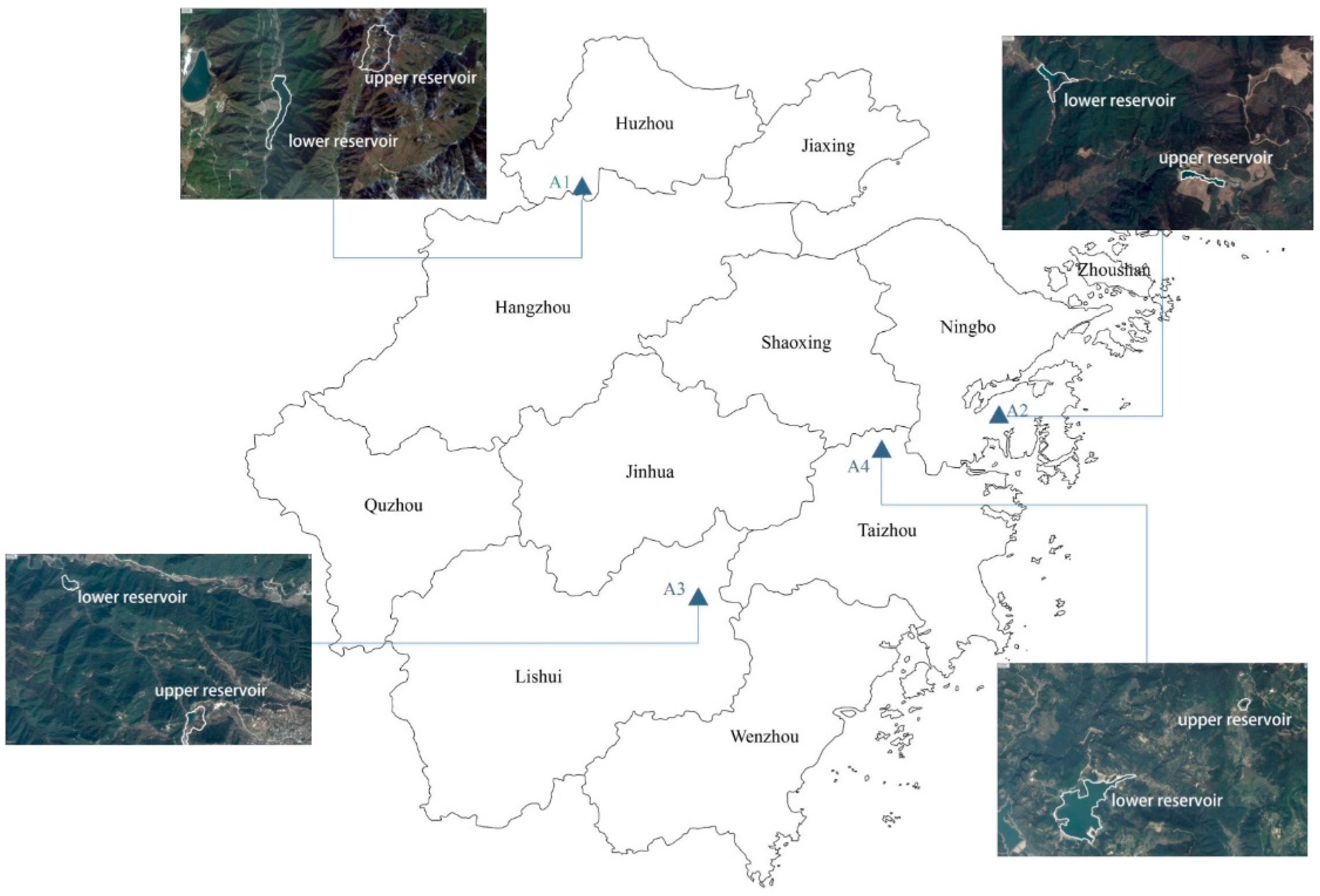
In April 2013, the NEA issued the “Reply on the pumped hydro energy storage plant location planning of Zhejiang province”, in which nine potential PHESP sites have been recommended. On further investigation, four promising PHES sites from these sites are selected using GIS technology. There are Changlongshan PHESP (30°28′21.68″ N, 119°37′28.30″ E), Ninghai PHESP (29°23′20.47″ N, 121°36′1.77″ E), Jinyun PHESP (28°31′32.77″ N, 120°10′31.82″ E), and Tiantai PHESP (29°13′30.17″ N, 121°02′39.18″ E). The distribution and general situation of the four sites are shown in Figure 3 To select the optimal one, the seven experts who were invited to screen criteria were invited again. Also, the second expert meeting was held. The main tasks of this meeting are to determine the weights of criteria and to define the evaluation scale of criteria values. After several rounds of consultation, the experts’ opinions tend to converge. The pair-wise comparison judgment matrices were collected. Also, the scales of the 2DULVs for each criteria were determined as and . As mentioned previously, the decision criteria values of PHESP site selection are heterogeneous. The relative data or information are collected and shown in Table 2. The performance numerical and triangular intuitionistic fuzzy numbers (TIFNs) values of the second type sub-criteria and the performance 2DUIVs values of the last type sub-criteria are shown in Table 3 and Table 4 respectively.
6.2. Sitting Decision-Making Process
Firstly, the normalized decision-making matrix composed by a mixture of CNVs, TIFNs, and 2DULVs is calculated and shown in Appendix B.
Secondly, the PIS and NIS are identified, and the separation of each alternative with respect to the PIS and NIS is calculated, which is shown in Table 5.
Thirdly, pair-wise comparison judgment matrices are provided by the experts (see Appendix C). Based on these matrices, the weights of criteria are obtained using the method of AHP, shown as follows:
- ;
- ; ;
- ; .
Fourthly, let the value of be 0.5, then the values , , and of each alternative are calculated, which is shown in Table 6.
Fifthly, the raking result can be obtained as by comparing value in an increasing order. Also, satisfies the conditions and , so it is considered as the optimal alternative.
6.3. Sensitivity Analysis
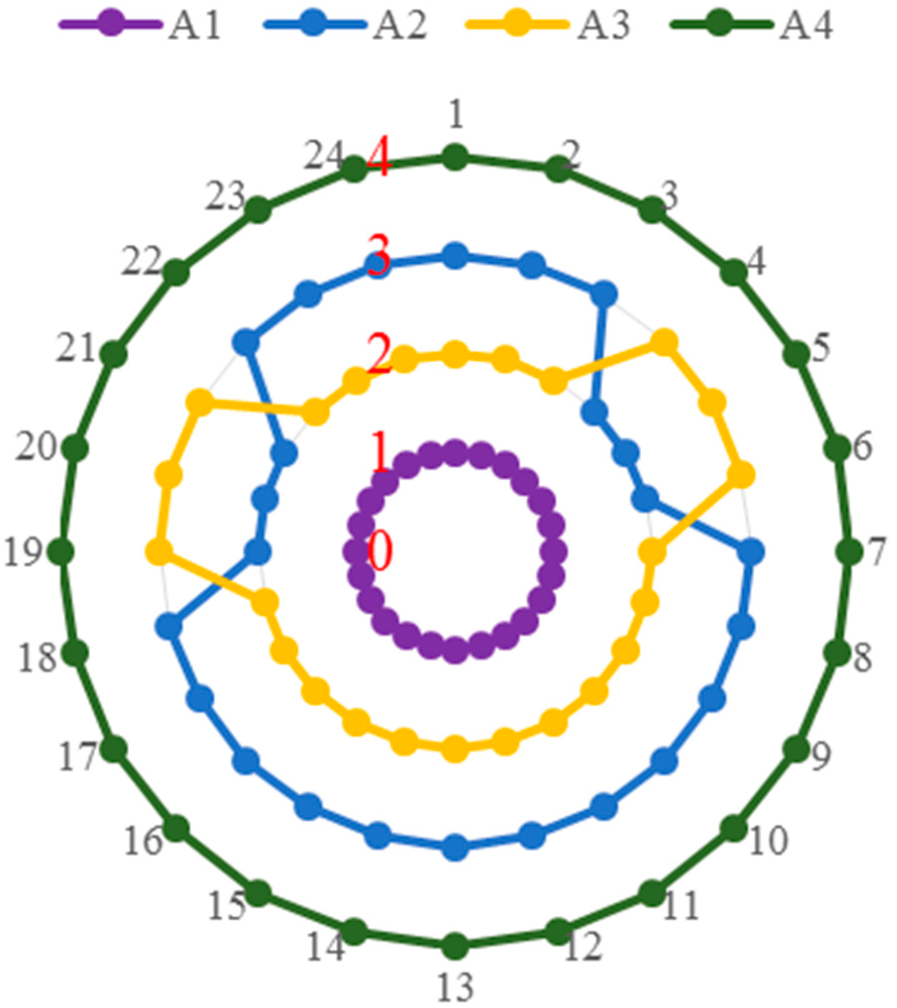
A sensitivity analysis is performed to test whether the ranking results would qualitatively change if the criteria weights fluctuated. Figure 4 shows those cases where the four criteria have 10%, 20%, and 30% less weight and 10%, 20%, and 30% more weight than the base weight. It can be seen that although the sequencing of alternative A2 and A3 is changeable, A1 is always the best alternative in all 24 tests. So it could be concluded that the method proposed in this study is effective and suitable for the optimal site selection of PHESP. In conclusion, the alternative A1 should be selected as the optimal PHESP site for construction in priority.
7. Conclusions
This paper establishes a VIKOR-based, multi-criteria site selection model for the PHESP site selection. This study has the following advantages compared with existing research: (i) it has constructed a comprehensive evaluation index system, which consists of four criteria and 15 sub-criteria, which reflects the inherent characteristics of PHESP site selection comprehensively; (ii) it can decrease the information distortion and losing that exists in criteria value representation and the information transformation process by considering the different properties of the criteria. When applied to a case from Zhejiang province, China, the decision model shows good suitability. This study provides a clear decision process for DMs to improve management efficiency. Moreover, the decision model could also be applied to solve other comprehensive and multi-criteria optimal location problems, such as tidal power station.
Although the proposed method in this paper helps improve the decision accuracy, there is still some room for improvement. It would be very interesting to extend our study to the case in a more sophisticated situation, such as introducing the behavior theory of DMs. Besides, this paper only considers the case that opinions of all experts arrive at a consensus. But, in some cases, the experts are divided in their opinions since they have different background knowledge. Thus, extending our study to group decision-making is meaningful work.
Acknowledgments
Project supported by the 2017 Special Project of Cultivation and Development of Innovation Base (No. Z171100002217024).
Author Contributions
Yunna Wu and Lingyun Liu designed the optimal PHESP site selection framework and Jianwei Gao mainly studied the proposed method. Then, Han Chu collected the relative data, calculated the result, and adjusted the format of the paper. Finally, Chuanbo Xu drafted the paper and formatted the manuscript for submission.
Conflicts of Interest
The authors declare no conflict of interest.
Appendix A
Appendix A.1. Terrain
The geological conditions should be suitable for the construction of a PHESP. It is the key to the PHESP site selection; the sub-criteria are mainly considered from two aspects: feasibility and capacity.
Appendix A.1.1. Permeability
Permeability is an important criterion for a PHESP; the upper reservoirs’ permeability is related to the energy conversion efficiency [42]. Also, it determined the operation maintenance cost of a pumped storage.
Appendix A.1.2. Altitude
The altitude refers to the deference of height of the upper and lower reservoirs [43]. During the operation of a PHESP, the level of the headwater had an important influence on the flow rate and unit efficiency.
Appendix A.1.3. Storage Capacity
Storage capacity refers to how much water the upper reservoir could hold. Electrical energy storage capacity is a traditional criterion for PHESP. Also, on the other hand, the lower reservoir must be large enough and have sufficient water for storage since it concerns the regulating ability of a PHESP [44].
Appendix A.1.4. Proximity to Electricity Grid
An electrical distribution station is one of the effective factors. Avoiding this industrial from of power transmission lines, in addition to the voltage dropping along the way, plus reducing the overall efficiency of industrial processes and wasting more energy, ultimately will lead to environmental pollution [42].
Appendix A.1.5. Length-Height Ratio
The horizontal distance between the upper reservoir and the lower reservoir L determines the length of the construction of the waterway; the waterway is too long and not only the project amount is large; the construction cost is also getting high, and the resistance of the water supply is large, which directly causes the head loss, so the upper reservoir and the next reservoir between the horizontal distance L is the second important condition of the street, in general L/H (distance ratio) to less than 10.
Appendix A.2. Economic Effect
As for economic effect, sub-criteria are determined from the internal economic assessment of the plants.
Appendix A.2.1. Loan Repayment Period
The loan payback period refers to the concrete in the fiscal and taxation policy and the enterprise financial conditions; the project can be used as a reimbursement of the profit after production, depreciation, and amortization, and other income can be used to repay the loan principal construction investment (including the construction period of unpaid interest) for the time required.
Appendix A.2.2. Assets Liabilities Ratio
It is the ratio of total debt (the sum of current liabilities and long-term liabilities) and total assets (the sum of current assets, fixed assets, and other assets such as ‘goodwill’).
Appendix A.2.3. Pay Back Period
Measures the length of the total project pay pack period. Under the Double-System Electricity Price of China, PHES is profitable, and the payback period should be taken into consideration.
Appendix A.2.4. Financial Internal Rate of Return
Refers to the fact that its calculation does not involve external factors, such as inflation or the cost of capital.
Appendix A.3. Social Benefits
A big construction project will influence the external environment, positively or negatively, and that must be considered. Furthermore, the ancillary services value of PHESP should be evaluated before the construction.
Appendix A.3.1. Employment
Evaluates the motivation to employment in relevant industries, including the manufacturing industry, transportation, etc. [17].
Appendix A.3.2. Economy improvement
Refers to the improvement of the local economy. Construction of a PHESP reaches up to several billions; it is a strong stimulant to the local economy [45].
Appendix A.3.3. Withstanding disasters
As a reservoir, the function of withstanding disaster is a basic function. Evaluating the capacity of withstanding a disaster such as a torrential flood is important for evaluating a PHESP roundly.
Appendix A.4. Environment
Environment is an important criterion for infrastructure construction. Sub-criteria in terms of environment are established to measure the decrease of the pollution gas emission.
Appendix A.4.1. Carbon Emission Reduction [46]
Evaluate the function of reducing the carbon emission. This research adopted the reforestation cost approach to evaluate the benefits of carbon emission reduction.
where is the environment benefits of the carbon emission by PHESP. is the weight of coal saving by PHESP. is the amount of carbon dioxide produced by burning a ton of standard coal. is the carbon price.
Appendix A.4.2. Nitrogen Oxide Emission
Evaluate the decrease of nitrogen oxide after the plant runs full out. The environmental benefit of the reduction of nitrogen oxide emission is calculated by the equation.
where is the environmental benefits of the discharges of nitrogen oxide by PHESP. is the unit of coal burning nitrogen oxide emissions. is the mass of the carbon emission of 1t standard coal.
Appendix A.4.3. Sulfur Dioxide Emission
Evaluate the decrease of sulfur dioxide after the plant runs full out. Because of the backward nature of the SO2 detection, this research adopted the material balance method.
where is the environmental benefits of the discharges of sulfur dioxide by PHESP. is the quality of coal saved using PHESP. is the rate of the sulfur transformed into sulfur dioxide. is the content of sulfur in coal. is the sulfur removal efficiency.
Appendix B
| Criteria | PIS | NIS | A1 | A2 | A3 | A4 | ||||
| d1j+ | d1j− | d1j+ | d1j− | d1j+ | d1j− | d1j+ | d1j− | |||
| C11 | A1 | A2 | 0 | 1 | 1 | 0 | 0.289 | 0.712 | 0.877 | 0.123 |
| C12 | A1 | A4 | 0 | 1 | 0.360 | 0.640 | 0.355 | 0.645 | 1 | 0 |
| C13 | A1 | A2 | 0 | 1 | 0.702 | 0.298 | 0.931 | 0.069 | 1 | 0 |
| C14 | A2 | A3 | 0.157 | 0.843 | 0 | 1 | 1 | 0 | 0.199 | 0.801 |
| C15 | A1 | A4 | 0.000 | 1.000 | 0.576 | 0.424 | 0.367 | 0.633 | 1 | 0 |
| C21 | A1 | A4 | 0 | 0.475 | 0.300 | 0.175 | 0.350 | 0.125 | 0.475 | 0 |
| C22 | A1 | A2 | 0 | 0.200 | 0.200 | 0 | 0.050 | 0.150 | 0.100 | 0.100 |
| C23 | A4 | A3 | 0.225 | 0.250 | 0.400 | 0.075 | 0.475 | 0 | 0 | 0.475 |
| C31 | A3 | A1 | 0.850 | 0.000 | 0.575 | 0.275 | 0 | 0.850 | 0.010 | 0.841 |
| C32 | A3 | A2 | 0.429 | 0.535 | 0.964 | 0 | 0 | 0.964 | 0.302 | 0.662 |
| C33 | A3 | A1 | 1.059 | 0.000 | 0.714 | 0.345 | 0 | 1.059 | 0.309 | 0.749 |
| C34 | A2 | A3 | 0.518 | 0.406 | 0 | 0.924 | 0.924 | 0 | 0.510 | 0.414 |
| C41 | A1 | A4 | 0 | 0.987 | 0.606 | 0.380 | 0.966 | 0.021 | 0.987 | 0 |
| C42 | A1 | A4 | 0 | 1.116 | 0.764 | 0.351 | 1.026 | 0.090 | 1.116 | 0 |
| C43 | A1 | A4 | 0 | 0.990 | 0.650 | 0.340 | 0.952 | 0.038 | 0.990 | 0 |
Appendix C
References
- Rogeau, A.; Girard, R.; Kariniotakis, G. A generic gis-based method for small pumped hydro energy storage (phes) potential evaluation at large scale. Appl. Energy 2017, 197, 241–253. [Google Scholar] [CrossRef]
- Akinyele, D.O.; Rayudu, R.K. Review of energy storage technologies for sustainable power networks. Sustain. Energy Technol. Assess. 2014, 8, 74–91. [Google Scholar] [CrossRef]
- Kong, Y.; Kong, Z.; Liu, Z.; Wei, C.; Zhang, J.; An, G. Pumped storage power stations in china: The past, the present, and the future. Renew. Sustain. Energy Rev. 2016, 71, 720–731. [Google Scholar] [CrossRef]
- Gimeno-Gutiérrez, M.; Lacal-Arántegui, R. Assessment of the european potential for pumped hydropower energy storage based on two existing reservoirs. Renew. Energy 2015, 75, 856–868. [Google Scholar] [CrossRef]
- Petrakopoulou, F.; Robinson, A.; Loizidou, M. Simulation and analysis of a stand-alone solar-wind and pumped-storage hydropower plant. Energy 2016, 96, 676–683. [Google Scholar] [CrossRef]
- Pérez-Díaz, J.I.; Jiménez, J. Contribution of a pumped-storage hydropower plant to reduce the scheduling costs of an isolated power system with high wind power penetration. Energy 2016, 109, 92–104. [Google Scholar] [CrossRef]
- Pérez-Díaz, J.I.; Chazarra, M.; García-González, J.; Cavazzini, G.; Stoppato, A. Trends and challenges in the operation of pumped-storage hydropower plants. Renew. Sustain. Energy Rev. 2015, 44, 767–784. [Google Scholar] [CrossRef]
- Yang, C.J.; Jackson, R.B. Opportunities and barriers to pumped-hydro energy storage in the united states. Renew. Sustain. Energy Rev. 2011, 15, 839–844. [Google Scholar] [CrossRef]
- Lu, X.; Wang, S. A gis-based assessment of tibet’s potential for pumped hydropower energy storage ☆. Renew. Sustain. Energy Rev. 2016, 69, 1045–1054. [Google Scholar] [CrossRef]
- Kucukali, S. Finding the most suitable existing hydropower reservoirs for the development of pumped-storage schemes: An integrated approach. Renew. Sustain. Energy Rev. 2014, 37, 502–508. [Google Scholar] [CrossRef]
- Connolly, D.; Maclaughlin, S.; Leahy, M. Development of a computer program to locate potential sites for pumped hydroelectric energy storage. Energy 2010, 35, 375–381. [Google Scholar] [CrossRef]
- Vasileiou, M.; Loukogeorgaki, E.; Vagiona, D.G. Gis-based multi-criteria decision analysis for site selection of hybrid offshore wind and wave energy systems in greece. Renew. Sustain. Energy Rev. 2017, 73, 745–757. [Google Scholar] [CrossRef]
- Düğenci, M. A new distance measure for interval valued intuitionistic fuzzy sets and its application to group decision making problems with incomplete weights information. Appl. Soft Comput. 2016, 41, 120–134. [Google Scholar] [CrossRef]
- Wu, Y.; Chen, K.; Zeng, B.; Yang, M.; Geng, S. Cloud-based decision framework for waste-to-energy plant site selection—A case study from china. Waste Manag. 2016, 48, 593–603. [Google Scholar] [CrossRef] [PubMed]
- Wu, Y.; Geng, S.; Zhang, H.; Gao, M. Decision framework of solar thermal power plant site selection based on linguistic choquet operator. Appl. Energy 2014, 136, 303–311. [Google Scholar] [CrossRef]
- Sánchez-Lozano, J.M.; García-Cascales, M.S.; Lamata, M.T. Gis-based onshore wind farm site selection using fuzzy multi-criteria decision making methods. Evaluating the case of southeastern spain. Appl. Energy 2016, 171, 86–102. [Google Scholar] [CrossRef]
- Wu, Y.; Zhang, J.; Yuan, J.; Geng, S.; Zhang, H. Study of decision framework of offshore wind power station site selection based on electre-iii under intuitionistic fuzzy environment: A case of china. Energy Convers. Manag. 2016, 113, 66–81. [Google Scholar] [CrossRef]
- Wu, Y.; Geng, S.; Xu, H.; Zhang, H. Study of decision framework of wind farm project plan selection under intuitionistic fuzzy set and fuzzy measure environment. Energy Convers. Manag. 2014, 87, 274–284. [Google Scholar] [CrossRef]
- Wu, Y.; Chen, K.; Zeng, B.; Yang, M.; Li, L.; Zhang, H. A cloud decision framework in pure 2-tuple linguistic setting and its application for low-speed wind farm site selection. J. Clean. Prod. 2017, 142, 2154–2165. [Google Scholar] [CrossRef]
- Zhu, W.D.; Zhou, G.Z.; Yang, S.L. An approach to group decision making based on 2-dimension linguistic assessment information. Syst. Eng. 2009, 27, 113–118. [Google Scholar]
- Xu, Z. Uncertain Linguistic Aggregation Operators Based Approach to Multiple Attribute Group Decision Making under Uncertain Linguistic Environment. Inf. Sci. 2004, 168, 171–184. [Google Scholar] [CrossRef]
- Liu, P. An approach to group decision making based on 2-dimension uncertain linguistic information. Technol. Econ. Dev. Economy 2012, 18, 424–437. [Google Scholar] [CrossRef]
- Liu, P.; Yu, X. 2-Dimension Uncertain Linguistic Power Generalized Weighted Aggregation Operator and Its Application in Multiple Attribute Group Decision Making. Knowl.-Based Syst. 2014, 57, 69–80. [Google Scholar] [CrossRef]
- Liu, P.; He, L.; Yu, X. Generalized hybrid aggregation operators based on the 2-dimension uncertain linguistic information for multiple attribute group decision making. Group Decis. Negot. 2016, 25, 103–126. [Google Scholar] [CrossRef]
- Liu, P.; Wang, Y. The aggregation operators based on the 2-dimension uncertain linguistic information and their application to decision making. Int. J. Mach. Learn. Cybern. 2016, 7, 1057–1074. [Google Scholar] [CrossRef]
- Wu, Y.; Xu, C.; Xu, H. Optimal site selection of tidal power plants using a novel method: A case in china. Energies 2016, 9, 832. [Google Scholar] [CrossRef]
- Matsui, O.; Kobayashi, G.S. Deriving preference order of open pit mines equipment through madm methods: Application of modified vikor method. Expert Syst. Appl. 2011, 38, 2550–2556. [Google Scholar]
- Sun, P.; Liu, Y.; Qiu, X.; Wang, L. Hybrid multiple attribute group decision-making for power system restoration. Expert Syst. Appl. 2015, 42, 6795–6805. [Google Scholar] [CrossRef]
- Hwang, C.L.; Yoon, K. Multiple Attribute Decision Making; Springer: Berlin/Heidelberg, Germany, 1981; pp. 287–288. [Google Scholar]
- Opricovic, S.; Tzeng, G.H. Extended vikor method in comparison with outranking methods. Eur. J. Oper. Res. 2007, 178, 514–529. [Google Scholar] [CrossRef]
- Opricovic, S.; Tzeng, G.H. Compromise solution by mcdm methods: A comparative analysis of vikor and topsis. Eur. J. Oper. Res. 2004, 156, 445–455. [Google Scholar] [CrossRef]
- Mousavi, S.M.; Jolai, F.; Tavakkoli-Moghaddam, R. A fuzzy stochastic multi-attribute group decision-making approach for selection problems. Group Decis. Negot. 2013, 22, 207–233. [Google Scholar] [CrossRef]
- Liu, H.C.; You, J.X.; You, X.Y.; Shan, M.M. A novel approach for failure mode and effects analysis using combination weighting and fuzzy vikor method. Appl. Soft Comput. J. 2015, 28, 579–588. [Google Scholar] [CrossRef]
- Mokhtarian, M.N.; Sadi-Nezhad, S.; Makui, A. A new flexible and reliable interval valued fuzzy vikor method based on uncertainty risk reduction in decision making process: An application for determining a suitable location for digging some pits for municipal wet waste landfill. Comput. Ind. Eng. 2014, 78, 213–233. [Google Scholar] [CrossRef]
- You, X.Y.; You, J.X.; Liu, H.C.; Zhen, L. Group multi-criteria supplier selection using an extended vikor method with interval 2-tuple linguistic information. Expert Syst. Appl. 2015, 42, 1906–1916. [Google Scholar] [CrossRef]
- Li, D.F. A ratio ranking method of triangular intuitionistic fuzzy numbers and its application to madm problems. Comput. Math. Appl. 2010, 60, 1557–1570. [Google Scholar] [CrossRef]
- Wan, S.P.; Wang, F.; Lin, L.L.; Dong, J.Y. Some new generalized aggregation operators for triangular intuitionistic fuzzy numbers and application to multi-attribute group decision making. Comput. Ind. Eng. 2016, 93, 286–301. [Google Scholar] [CrossRef]
- Liu, P. The research note of 2-dimension uncertain linguistic variables. Shandong Univ. Financ. Econ. 2012, 9, 20. [Google Scholar]
- Opricovic, S. Multicriteria Optimization of Civil Engineering Systems. Ph.D. Thesis, Faculty of Civil Engineering, Belgrade, Serbia, 1998. [Google Scholar]
- Kumar, M.; Samuel, C. Selection of best renewable energy source by using VIKOR method. Technol. Econ. Smart Grids Sustain. Energy 2017, 2. [Google Scholar] [CrossRef]
- Jiang, Z.; Zhang, H.; Sutherland, J.W. Development of multi-criteria decision making model for remanufacturing technology portfolio selection. J. Clean. Prod. 2011, 19, 1939–1945. [Google Scholar] [CrossRef]
- Capilla, J.A.J.; Carrión, J.A.; Alameda-Hernandez, E. Optimal site selection for upper reservoirs in pump-back systems, using geographical information systems and multicriteria analysis. Renew. Energy 2016, 86, 429–440. [Google Scholar] [CrossRef]
- Zhao, H.; Feng, Y.; Zhang, X.; Zhen, R. Hydro-thermal unit commitment considering pumped storage stations. In Proceedings of the International Conference on Power System Technology, Beijing, China, 18–21 August 1998; pp. 576–580. [Google Scholar]
- Connolly, D.; Lund, H.; Finn, P.; Mathiesen, B.V.; Leahy, M. Practical operation strategies for pumped hydroelectric energy storage (PHES) utilising electricity price arbitrage. Energy Policy 2011, 39, 4189–4196. [Google Scholar] [CrossRef]
- Deane, J.P.; Gallachóir, B.P.Ó.; Mckeogh, E.J. Techno-economic review of existing and new pumped hydro energy storage plant. Renew. Sustain. Energy Rev. 2010, 14, 1293–1302. [Google Scholar] [CrossRef]
- Zhang, N.; Lu, X.; Mcelroy, M.B.; Nielsen, C.P.; Chen, X.; Deng, Y.; Kang, C. Reducing curtailment of wind electricity in china by employing electric boilers for heat and pumped hydro for energy storage. Appl. Energy 2016, 184, 987–994. [Google Scholar] [CrossRef]
Figure 1.
Installed capacity of various storage technologies in global electricity storage system (Unit: MW, Sources: Report issued by the International Renewable Energy Agency—“Re-Thinking Energy 2017”).
Figure 1.
Installed capacity of various storage technologies in global electricity storage system (Unit: MW, Sources: Report issued by the International Renewable Energy Agency—“Re-Thinking Energy 2017”).

Figure 2.
A TIFN .

Figure 3.
Distribution and general situation of the four sites.

Figure 4.
Ranking results of changing the four criteria weight.


Table 1.
The criteria and sub-criteria of PHESP site selection.
| Criteria | Symbol | Sub-Criteria | Symbol |
|---|---|---|---|
| Terrain and geography | C1 | Permeability | C11 |
| Altitude | C12 | ||
| Storage capacity | C13 | ||
| Proximity to electricity grid | C14 | ||
| Length-height ratio | C15 | ||
| Social effect | C2 | Employment | C21 |
| Economy improvement | C22 | ||
| Disasters withstand | C23 | ||
| Economic effect | C3 | Loan repayment period | C31 |
| Assets liabilities ratio | C32 | ||
| Pay back period | C33 | ||
| Financial internal rate of return | C34 | ||
| Environmental effect | C4 | Carbon emission reduction | C41 |
| Nitrogen oxide emission reduction | C42 | ||
| Sulfur dioxide emission reduction | C43 |
Table 2.
Performance numerical values of the first type sub-criteria.
| Alternative | C11 (m/h) | C12 (m) | C13 (m2) | C14 (m) | C15 |
|---|---|---|---|---|---|
| A1 | 339.45 | 567 | 99,152 | 4258 | 2.49 |
| A2 | 570.46 | 485 | 34,493 | 3692 | 5.42 |
| A3 | 405.94 | 486 | 13,457 | 7307 | 4.36 |
| A4 | 542.16 | 339 | 7102 | 4412 | 7.59 |
Table 3.
Performance numerical and triangular intuitionistic fuzzy numbers (TIFNs) values of the second type sub-criteria.
Table 3.
Performance numerical and triangular intuitionistic fuzzy numbers (TIFNs) values of the second type sub-criteria.
| Alternative | C31 (a) | C32 | C33 (a) | C34 | C41 (10 × 4CNY) | C42 (10 × 4CNY) | C43 (10 × 4CNY) | |
|---|---|---|---|---|---|---|---|---|
| A1 | Value | ≈8.5 | ≈75.35 | ≈13.6 | ≈17.56 | ≈2530 | ≈4208 | ≈406 |
| TIFN | ((8.3, 8.5, 8.7); 0.7, 0.1) | ((75.21, 75.35, 75.46); 0.7, 0.1) | ((13.5, 13.6, 13.8); 0.7, 0.2) | ((17.4, 17.56, 17.7); 0.6, 0.3) | ((2518, 2530, 2543); 0.7, 0.2) | ((4187, 4208, 4223); 0.8, 0.1) | ((389, 406, 419); 0.8, 0.2) | |
| A2 | Value | ≈9.8 | ≈70.35 | ≈15.7 | ≈19.62 | ≈1246 | ≈2106 | ≈210 |
| TIFN | ((9.5, 9.8, 9.8); 0.8, 0.1) | ((70.12, 70.35, 70.43); 0.8, 0.2) | ((15.5, 15.7, 15.8); 0.6, 0.3) | ((19.5, 19.62, 19.7); 0.7, 0.2) | ((1230, 1246, 1261); 0.8, 0.1) | ((2092, 2106, 2122); 0.7, 0.1) | ((198, 210, 223); 0.7, 0.2) | |
| A3 | Value | ≈13.2 | ≈80 | ≈18.4 | ≈15.33 | ≈623 | ≈1362 | ≈108 |
| TIFN | ((12.9, 13.2, 13.4); 0.6, 0.2) | ((79.83, 80, 80.15); 0.7, 0.2) | ((18.1, 18.4, 18.6); 0.8, 0.1) | ((15.1, 15.33, 15.5); 0.9, 0.1) | ((609, 623, 642); 0.7, 0.1) | ((1254, 1362, 1378); 0.7, 0.2) | ((98, 108, 121); 0.8, 0.2) | |
| A4 | Value | ≈12.8 | ≈78 | ≈17.2 | ≈16.97 | ≈589 | ≈1052 | ≈96 |
| TIFN | ((12.6, 12.8, 13); 0.7, 0.2) | ((77.9, 78, 78.17); 0.6, 0.3) | ((17.1, 17.2, 17.3); 0.8, 0.2) | ((16.9, 16.97, 17.2); 0.8, 0.1) | ((573, 589, 603); 0.6, 0.3) | ((1013, 1052, 1070); 0.8, 0.1) | ((87, 96, 106); 0.8, 0.1) | |
Table 4.
Performance 2DUIVs values of the last type sub-criteria.
| Alternative | C21 | C22 | C23 |
|---|---|---|---|
| A1 | (S2, S3), (S1, S2) | (S2, S3), (S1, S2) | (S1, S3), (S1, S2) |
| A2 | (S1, S2), (S1, S2) | (S1, S2), (S0, S1) | (S2, S3), (S0, S1) |
| A3 | (S3, S4), (S0, S1) | (S1, S2), (S1, S2) | (S0, S1), (S1, S2) |
| A4 | (S1, S2), (S0, S1) | (S3, S4), (S0, S1) | (S3, S4), (S1, S2) |
Table 5.
The separation of each alternative from positive and negative ideal solution.
| Criteria | PIS | NIS | A1 | A2 | A3 | A4 | ||||
|---|---|---|---|---|---|---|---|---|---|---|
| d1j+ | d1j− | d1j+ | d1j− | d1j+ | d1j− | d1j+ | d1j− | |||
| C11 | A1 | A2 | 0 | 1 | 1 | 0 | 0.289 | 0.712 | 0.877 | 0.123 |
| C12 | A1 | A4 | 0 | 1 | 0.360 | 0.640 | 0.355 | 0.645 | 1 | 0 |
| C13 | A1 | A2 | 0 | 1 | 0.702 | 0.298 | 0.931 | 0.069 | 1 | 0 |
| C14 | A2 | A3 | 0.157 | 0.843 | 0 | 1 | 1 | 0 | 0.199 | 0.801 |
| C15 | A1 | A4 | 0.000 | 1.000 | 0.576 | 0.424 | 0.367 | 0.633 | 1 | 0 |
| C21 | A1 | A4 | 0 | 0.475 | 0.300 | 0.175 | 0.350 | 0.125 | 0.475 | 0 |
| C22 | A1 | A2 | 0 | 0.200 | 0.200 | 0 | 0.050 | 0.150 | 0.100 | 0.100 |
| C23 | A4 | A3 | 0.225 | 0.250 | 0.400 | 0.075 | 0.475 | 0 | 0 | 0.475 |
| C31 | A3 | A1 | 0.850 | 0.000 | 0.575 | 0.275 | 0 | 0.850 | 0.010 | 0.841 |
| C32 | A3 | A2 | 0.429 | 0.535 | 0.964 | 0 | 0 | 0.964 | 0.302 | 0.662 |
| C33 | A3 | A1 | 1.059 | 0.000 | 0.714 | 0.345 | 0 | 1.059 | 0.309 | 0.749 |
| C34 | A2 | A3 | 0.518 | 0.406 | 0 | 0.924 | 0.924 | 0 | 0.510 | 0.414 |
| C41 | A1 | A4 | 0 | 0.987 | 0.606 | 0.380 | 0.966 | 0.021 | 0.987 | 0 |
| C42 | A1 | A4 | 0 | 1.116 | 0.764 | 0.351 | 1.026 | 0.090 | 1.116 | 0 |
| C43 | A1 | A4 | 0 | 0.990 | 0.650 | 0.340 | 0.952 | 0.038 | 0.990 | 0 |
Table 6.
Values of , , and of each alternative.
| Alternative | Value | Alternative | Value | Alternative | Value | |||
|---|---|---|---|---|---|---|---|---|
| A1 | 0.127 | A1 | 0.059 | A1 | 0 | |||
| A2 | 0.668 | A2 | 0.207 | A2 | 0.883 | |||
| A3 | 0.629 | A3 | 0.194 | A3 | 0.810 | |||
| A4 | 0.813 | A4 | 0.211 | A4 | 1 |
© 2017 by the authors. Licensee MDPI, Basel, Switzerland. This article is an open access article distributed under the terms and conditions of the Creative Commons Attribution (CC BY) license (http://creativecommons.org/licenses/by/4.0/).
Share and Cite
MDPI and ACS Style
Wu, Y.; Liu, L.; Gao, J.; Chu, H.; Xu, C. An Extended VIKOR-Based Approach for Pumped Hydro Energy Storage Plant Site Selection with Heterogeneous Information. Information 2017, 8, 106. https://doi.org/10.3390/info8030106
AMA Style
Wu Y, Liu L, Gao J, Chu H, Xu C. An Extended VIKOR-Based Approach for Pumped Hydro Energy Storage Plant Site Selection with Heterogeneous Information. Information. 2017; 8(3):106. https://doi.org/10.3390/info8030106
Chicago/Turabian StyleWu, Yunna, Lingyun Liu, Jianwei Gao, Han Chu, and Chuanbo Xu. 2017. "An Extended VIKOR-Based Approach for Pumped Hydro Energy Storage Plant Site Selection with Heterogeneous Information" Information 8, no. 3: 106. https://doi.org/10.3390/info8030106
Note that from the first issue of 2016, this journal uses article numbers instead of page numbers. See further details here.