Using OpenStreetMap Data and Machine Learning to Generate Socio-Economic Indicators


1
Institute of Spatial and Regional Planning, University of Stuttgart, 70569 Stuttgart, Germany
2
Administration de la Gestion de l’eau, Ministère de l’Environnement, du Climat et du Développement Durable, 4361 Esch-sur-Alzette, Luxembourg
3
Department of Ecology, Ecosystem and Landscape Ecology, University of Innsbruck, 6020 Innsbruck, Austria
*
Author to whom correspondence should be addressed.
ISPRS Int. J. Geo-Inf. 2020, 9(9), 498; https://doi.org/10.3390/ijgi9090498
Submission received: 1 May 2020
/
Revised: 4 August 2020
/
Accepted: 19 August 2020
/
Published: 21 August 2020
(This article belongs to the Special Issue OpenStreetMap as A Multi-Disciplinary Nexus: Perspectives, Practices and Procedures)
Abstract
:Socio-economic indicators are key to understanding societal challenges. They disassemble complex phenomena to gain insights and deepen understanding. Specific subsets of indicators have been developed to describe sustainability, human development, vulnerability, risk, resilience and climate change adaptation. Nonetheless, insufficient quality and availability of data often limit their explanatory power. Spatial and temporal resolution are often not at a scale appropriate for monitoring. Socio-economic indicators are mostly provided by governmental institutions and are therefore limited to administrative boundaries. Furthermore, different methodological computation approaches for the same indicator impair comparability between countries and regions. OpenStreetMap (OSM) provides an unparalleled standardized global database with a high spatiotemporal resolution. Surprisingly, the potential of OSM seems largely unexplored in this context. In this study, we used machine learning to predict four exemplary socio-economic indicators for municipalities based on OSM. By comparing the predictive power of neural networks to statistical regression models, we evaluated the unhinged resources of OSM for indicator development. OSM provides prospects for monitoring across administrative boundaries, interdisciplinary topics, and semi-quantitative factors like social cohesion. Further research is still required to, for example, determine the impact of regional and international differences in user contributions on the outputs. Nonetheless, this database can provide meaningful insight into otherwise unknown spatial differences in social, environmental or economic inequalities.
1. Introduction
In current policy and research on adaptation to climate change, resilience and vulnerability are key concepts for understanding the human dimension of strategies and measures to adapt to global change.
Vulnerability is a society’s inability to act and hence influence the impacts of global change on its people’s wellbeing. Increasing the resilience of societies, reducing disaster risk, and hence reducing the impacts of climate change, requires consideration of the social aspects of sustainable development and tackling causes, not symptoms. Socio-economic indicators are important measures to assess spatial or societal dimensions. Factors such as people’s economic or employment status are considered to influence their adaptation and coping capacity [1,2,3,4].
Although official socio-economic data from governmental and non-governmental institutions are reliable, comprehensive, and often the best choice to describe societal phenomena, they are only available at specific temporal and spatial resolutions and lack standardization between administrative levels, even within countries. Huge efforts to address this include, for example, the INSPIRE directive of the European Commission with a vision of unprecedented sharing of geospatial data. However, this initiative has not been able to reach its full potential yet, due to many barriers to its implementation [5]. Until now, elaborate surveys have often been necessary to generate knowledge about societal relationships with the natural, cultural, and economic environment.
The growing amount of data, open data policies, and crowd-sourced data has led to an increased availability and accessibility of socio-economic indicators. Nevertheless, the measurement of complex multifaceted phenomena (e.g., resilience, vulnerability, sustainability, adaptation) is still often limited due to unavailability of data [2,4,6,7]. Hence, the need for methods that allow deriving indicators from data sources, that are permanently available and offer spatially scalable information, has become very clear.
In recent years, artificial intelligence, and especially machine learning methods, have been developed and tested in many scientific disciplines in order to predict social characteristics and structures by analyzing implicit patterns in data of the observed systems. Random forest (RF) is one machine learning algorithm widely applied for geodata: e.g., for land cover classification from openly available geodata sets [8], mapping vegetation morphology types [9], habitat prediction of fisher (Pekania pennanti) [10], a multi-data approach to enhance crop classification [11], or downscaling census data [12]. Another machine learning algorithm applied across disciplines is neural networks (NN). Examples are seismic vulnerability assessment [13], modeling of the surface of the sea floor [14], flood hazard assessment [15], and analyzing land pattern evolution [16]. Within machine learning, neural networks belong to the deep learning category.
This research aimed to develop a machine learning approach to deduce socio-economic indicators from OpenStreetMap (OSM) for municipalities. The underlying hypothesis was that there are proxies for socio-economic attributes within the geodata of the OSM database. For example, can park benches be a predictor for an elderly population? Can the size of industrial areas or density of public transportation or infrastructure provide an indication of unemployment rates? Is nature or industry more predictive for migration? With four indicators (residents, unemployment, migration, and elderly) selected based on official statistical data, we tested the suitability of OSM as a data source and compare the predictive performance of three approaches: (1) random prediction as a baseline with linear regression; (2) one machine learning algorithm; and (3) one deep learning algorithm. We assessed the predictive power of each approach by comparing them to the testing regions where we know the actual situation.
This research paper is based on earlier investigations by the authors [17,18] and represents a refined approach to the analysis of the OSM database with artificial intelligence (AI). Section 2 introduces the study area and develops the methodology adopted, including the target indicators and the machine learning algorithms exploited. Section 3 presents the prediction results of the models, including a comparative performance evaluation. Section 4 discusses the findings in regard to each indicator and cross-cutting challenges amongst them, leading to opportunities for future research. Section 5 concludes by summarizing the research question and main results.
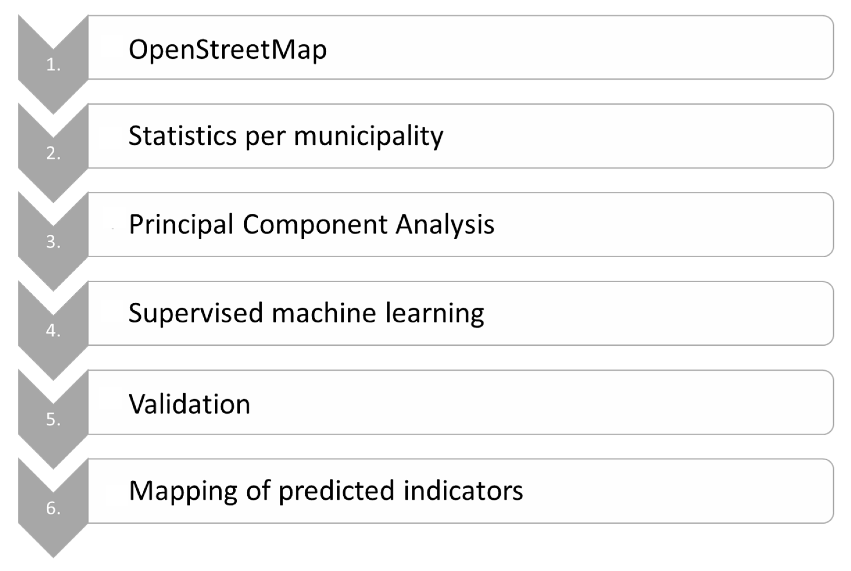
2. Method
The workflow follows the narrative of the research (Figure 1). Firstly, the OSM dataset was downloaded. Secondly, in a spatial query everything within the area of a municipality was counted. Thirdly, in a data processing step, a principal component analysis (PCA) was conducted to reduce the number of dimensions, resulting in uncorrelated principal components as indicator candidates. Fourthly, the indicator candidates were subsequently used to predict the four socio-economic indicators (unemployment, residents, migration, elderly). Fifthly, the model results were validated and, lastly, they were mapped.
In the following section, the case study and the selected socio-economic indicators are firstly described. Secondly, OSM is described as the data source with its key characteristics and implications for calculating spatial attributes for each municipality. Thirdly, the machine learning algorithms and their implementation, functions, and settings are discussed.
2.1. Test Region
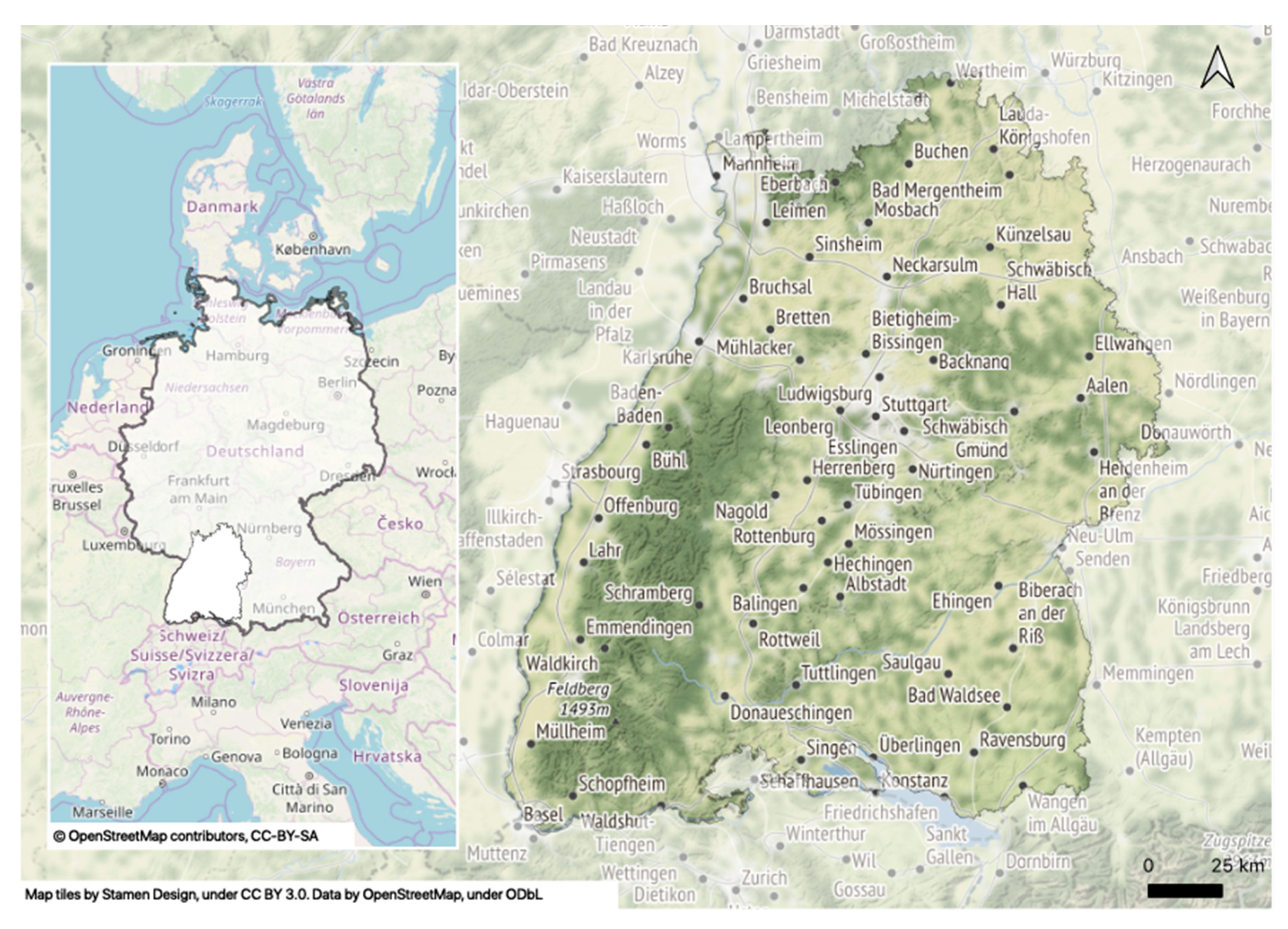
As a compromise between computational resources, data handling, and model complexity, the regional scale was chosen. Baden-Württemberg is the south-western federal state of Germany bordering France in the west and Switzerland in the south (Figure 2). The administrative territory with a size of 35,751.46 km2 is subdivided into four administrative districts (Regierungsbezirke) which contain 35 counties (Landkreise) and nine independent cities (Stadtkreise). In total, there are 1101 municipalities populated with around 11 million inhabitants. The density of the population is 310 inhabitants per km2, higher than that of Germany overall which is 232 inhabitants per km2 [19]. Economically, Baden-Württemberg is one of the strongest regions in Europe and is ranked third in Germany in terms of purchasing power after Hamburg and Bavaria [20]. Family-owned businesses are typical for the region. The overall unemployment rate is 3.1% and lower in rural areas [21]. In 2018, the average age was 43.5 years, an increase of 9 years from 1970. Although there has been considerable emigration of young people, the number has not changed much in recent years [22]. Currently, 294,000 people are 85 years or older. This is six times higher than in 1970. The current forecast expects the number to increase up to 805,000 people by 2060 [23].
2.2. Selected Socio-Economic Indicators
The selected socio-economic indicators for the purpose of this study were: (a) residents; (b) unemployment; (c) elderly; and (d) migration. Residents refers to the number of inhabitants per municipality. Unemployment refers to the percentage of unemployed people as part of the total number of employable people. The proportion of elderly people gives the percentage of people older than 65 years as part of the total population. Migration is calculated by subtracting emigration from immigration. A positive balance means that more people moved in to the municipality than out of it. These four metrics explain societal and economic conditions and are a common basis for many socio-economic indicators and of relevance for assessing and evaluating complex phenomena such as resilience, vulnerability, and sustainability [6,24,25,26].
2.3. OpenStreetMap—Developing Spatial Features for Municipalities
OSM is a free and collaborative project founded in 2004 [27]. The goal of the project is to create an open access map of the world. All elements of a topographic map, such as houses, streets, railways, and forests are mapped by volunteers around the globe [28]. Crowdsourced data are made public under the Open Database License. Current statistics show more than six million registered users, 5.75 billion nodes, and 3.5 million map changes per day [29].
Every element is described within the database by at least one tag in plain text. The tag consists of a key and a value. The key can describe the represented objects with the functional characteristics or other attributes such as names or owner. The keys are unique and categorical (e.g., land use) and describe the classes or domains that each object belongs to. Values can be used to further specify individual characteristics and explanations (e.g., tag: key = landuse; value = farmland).
For the purpose of this study, we first downloaded the full OSM dataset for the federal state of Baden-Württemberg from the Geofabrik website (https://download.geofabrik.de; October 2019). The downloaded .pbf file was then imported into a PostgreSQL database with PostGIS extension using osm2pgsql (https://github.com/openstreetmap/osm2pgsql). During the import, an initial data reduction took place through the used default import “style”, which excludes certain keys and additional information without explanatory relevance from the dataset. The resulting PostGIS geometry and attribute tables (point, line and polygon) contained 60 of the most relevant keys as columns and respective values as rows. In a further pre-processing step, the OSM data were intersected with the administrative boundaries of the municipalities within the federal state. Consequently, the sums of the geometries (area and length) and point counts for each occurrence of a unique key-value-pair were computed with SQL-queries for every municipality, resulting in a table with 1101 rows, each row representing one sample, meaning one municipality (Table 1).
The previous steps resulted in three distinct layers (points, lines, polygons), with the keys and values and the respective sums of their observed spatial occurrence (count, sqm, km). Each line or sample counted for one spatial feature, and therefore, there was an unrestricted number of lines per tag per municipality. All the following steps were conducted using R with R Studio [30,31] (additional packages: “tidyr”; “dplyr” [32,33]). The three tables were imported into R Studio from the PostGIS database (function: dbReadTable(); package: “RPostgres” [34]). In a preliminary data cleaning step, six keys (addr, name, xmas, contact, TMS, openGeoDB) were removed, as they did not contain relevant information for the task ahead. Moreover, only tags appearing in 100 or more municipalities were considered. The key and value columns were then joined to one tag column. Afterwards, the tags were aggregated by sum per municipality and written into one column per tag (function: dcast(); package: “reshape2” [35]). The same steps were taken for the three tables (points, lines, polygons), and the resulting tables were joined by the municipality code to one table. In the next step, these raw data were pre-processed for the machine learning part.
The population of the municipality as well as the area were imported (function: read_excel(); package: “readxl” [36]). The data set was split rather cautiously via random number generation into 50% test municipalities and 50% training municipalities to test the predictive power and increase generalization. To adjust for the different sizes of municipalities, the predictors were set into relation per 1000 capita. The training data were standardized and PCA conducted (function: preProcess(); package: “caret” [37]). The pre-process parameters from the training data were also taken for the test data so as to not blend in future information into the training process via standardization of the entire data set. The PCA was used to reduce dimensions and to have a set of uncorrelated indicator candidates to predict the four socio-economic indicators (see Appendix A).
2.4. Machine Learning to Predict Socio-Economic Indicators
The following section describes the predictive algorithms and their R functions that were applied to this analysis, including model parameters. Firstly, the baseline was established by random prediction and a linear model. Secondly, random forest and deep neural networks (DNN) were applied as a machine learning and deep learning approach. Thirdly, these models were compared to the ground truth and evaluated for predictive power.
For the random prediction (RP), random values within the range of the test data were generated. The mean absolute error (MAE) on the test data was calculated and compared as a baseline. The MAE was selected to test for model performance, which is reported in Table 2. The mean squared error (MSE) was neglected due to the potential overestimation of model performance as all outcome values were min–max normalized for comparison among them. Hence, calculating the square of values between zero and one would have resulted in significantly smaller absolute values and obscured the performance.
Linear regression (LR) was conducted as a basic statistic prediction method to better understand the performance of the machine learning algorithms (function: lm(); package: R base library).
Random forest (RF) is a machine learning algorithm based on the statistic of decision trees. In a randomized learning process, multiple uncorrelated decision trees are calculated. In the standard setting, 500 trees are built by subsets of the predictors to avoid the dominance of one very strong predictor (function: randomForest(); package: randomForest [38]). The importance of assessment of the predictors is set to true for detecting relevant predictors. The relevance of the predictors is determined by their contribution in reducing the test error over all trees.
Artificial neural networks are machine learning algorithms that function in a similar way to the human brain. A number of hidden layers and nodes, structure, organize, and detect patterns within data. Multiple sequential models are trained with a maximum of four hidden layers and 256 nodes for each of the four indicators (function: sequential(); package: “keras” [39]). Finally, the best four DNN, one for each indicator, with the lowest MAEs are selected.
Within the keras package, no method is yet included to assess the predictor importance and analyze the black box of the neural network. Similar to the random forest recording of the contribution to the reduction of the error, the permutation feature importance (PFI) was implemented. Here, the approach by Fioruzi (2018) was adopted, which is based on [40,41]. Although methodologically not defined, the method was implemented on the test data. For each predictor, the values are randomly permutated and the error of the neural network calculated. Afterwards, the absolute PFI was calculated by subtracting the original model error from the permutation error, resulting in a value about the contribution of the predictor on the reduction of the MAE.
The method described above was performed for all four outcomes, split into the same test and training sets. The final mapping of the indicators was done implementing a quantile classification with eight classes.
3. Results
The following section starts with the overall comparison of the performance of all applied machine learning algorithms on the four indicators. Subsequently, the spatial distribution and predictive elements of OSM for each indicator are presented.
3.1. Comparison of Machine Learning Algorithms and Model Performance
The first column represents the resulting MAE for randomly predicting values to establish the baseline for comparison (Table 2). The second, third, and fourth columns are the LR, RF, and DNN errors. In general, linear regression was better than random prediction, RF was better than LR, and DNN was better than RF. For the DNN model, the number of residents per municipality was best predicted with the lowest error, followed by migration, elderly, and unemployment.
3.2. Spatial Features of Number of Residents
The number of residents of each municipality was in decreasing order of the MAE modeled by random, linear, RF, and best DNN.
The DNN model clearly outperformed the RF model but resulted in the challenge of understanding the model. Performing the feature performance index (PFI), the four most important predictors of residents were (Table 3): Train system, Infrastructure, Shopping and culture, and Rurality.
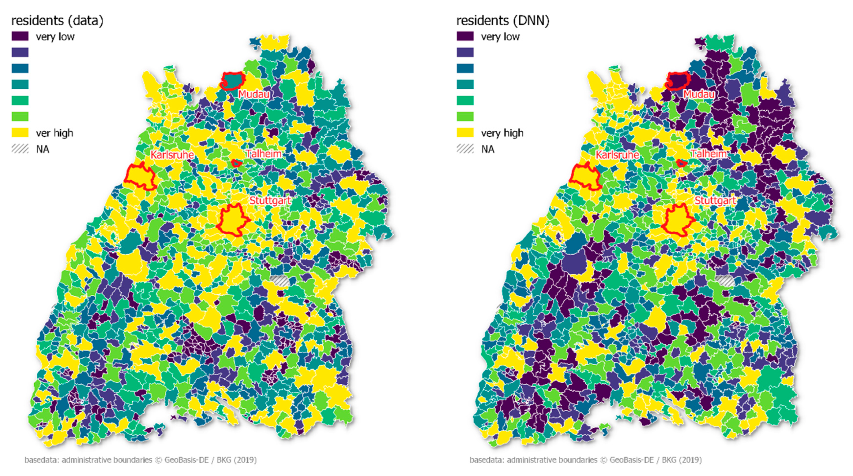
The highest error was for the state capital of Stuttgart (Figure 3). In fact, Stuttgart was not part of the training data and had a normalized value of over two due to its unmatched size within the training set. The DNN model failed to extrapolate the extraordinary size of the capital from the training data. This is the difficulty of the min–max normalization, which can result in test data values not seen within the training data. Additionally, the city of Karlsruhe emerged as having one of the worst predictions, which again shows the difficulties that the model has in making predictions for relatively large cities compared to the majority of smaller municipalities. Mudau and Talheim, with 5009 and 4830 inhabitants respectively, achieved the lowest errors. The mean number of residents over all 1101 municipalities in Baden-Württemberg is 10,054. Hence, the model performs well around the median and less well in predicting outliers. The areas without value (NA) do not have the legal administrative status of a municipality and are therefore not included in the statistics.
3.3. Predictors of Unemployment
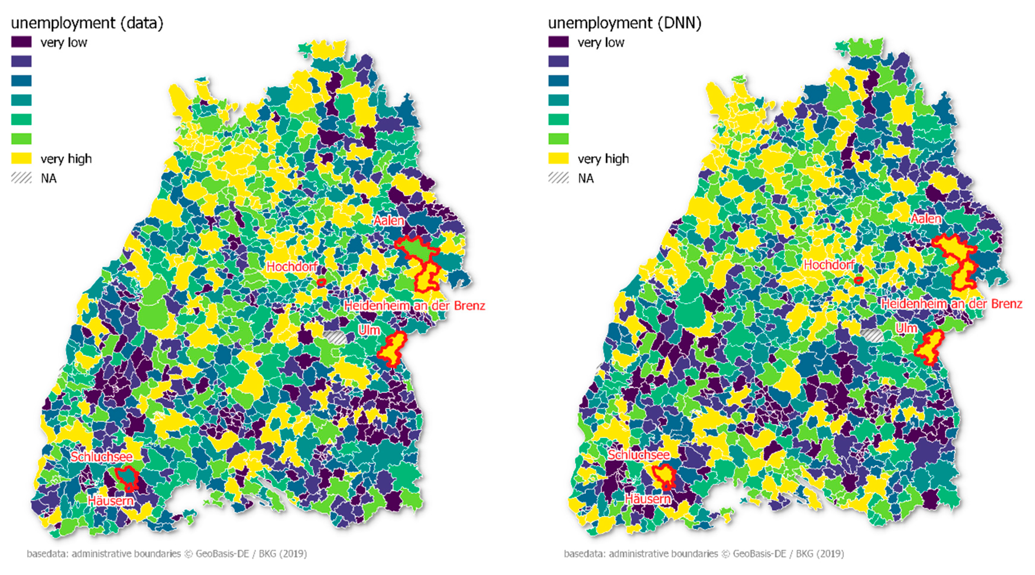
The level of unemployment as a share of the total population per municipality was the most difficult to predict compared to the other socio-economic indicators. Additionally, there was not much difference between DNN and RF. There is close to full employment throughout the entire federal state, with many hidden champions in the countryside. This explains the lower unemployment of rural regions compared to metropolitan areas (Figure 4).
The PCA of Tourism scored the highest PFI, followed by Natural sights, Historic rural, Train system, and Social care (Table 4). Hence, PCAs describing the typology of the municipality dominated. Schluchsee, located in the Black Forest, showed the highest error among all municipalities.
The prediction overestimated the unemployment in the municipality. The second highest MAE was reported for Heidenheim an der Brenz, where the real unemployment was underestimated. Interestingly, in the spatial proximity of Heidenheim, Ulm had the lowest error, followed by Hochdorf, Häusern, and Aalen.
3.4. Predictive Features for the Proportion of Elderly People
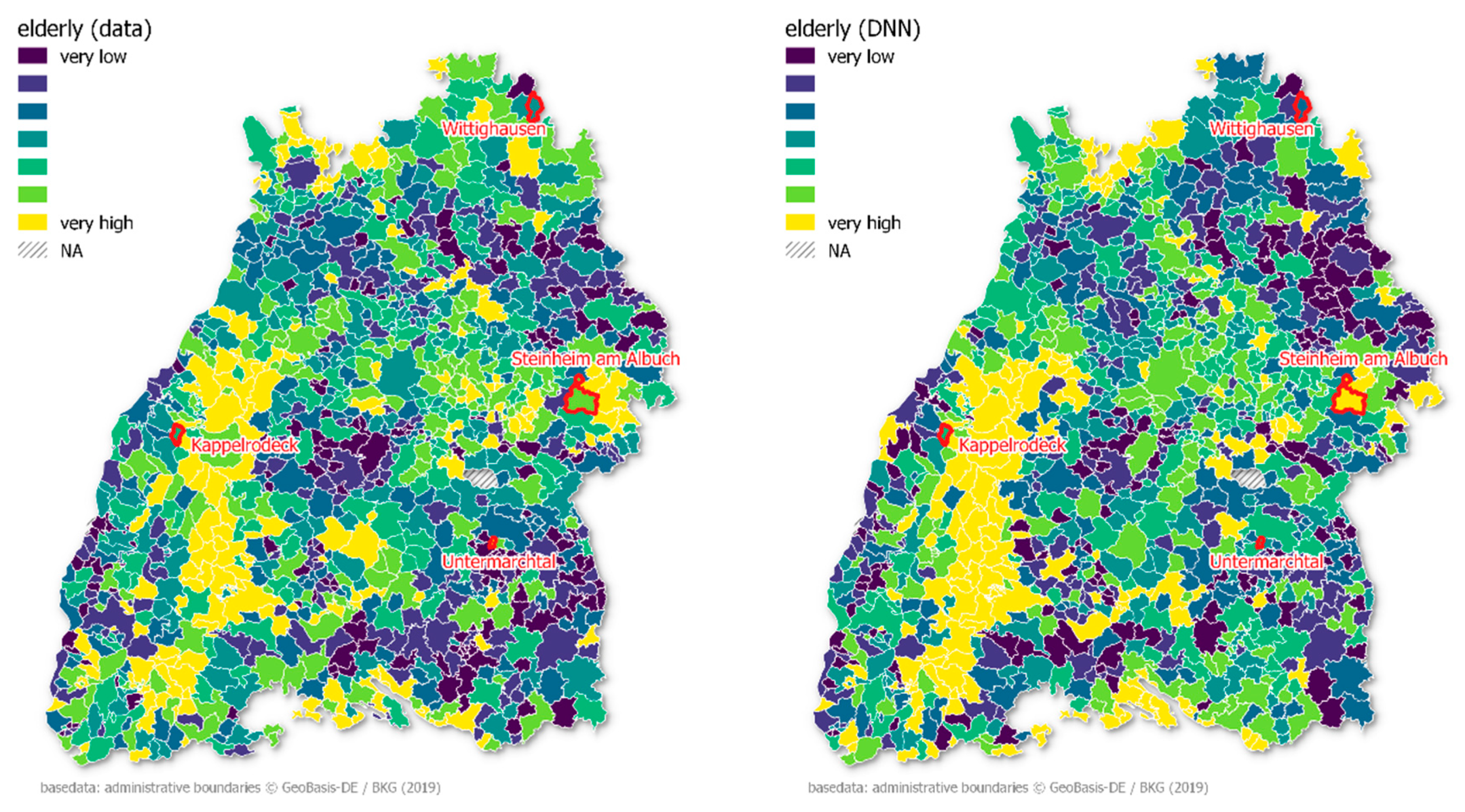
The proportion of elderly people in the municipality was modeled slightly better than unemployment. Again, there was only a marginal difference between RF and DNN, though both were superior to the linear model (Table 2). Across Baden-Württemberg, there is no clear pattern between rural and metropolitan areas (Figure 5). In the western Black Forest region, the share of older people is comparatively high, whereas in the north of Stuttgart and in the south-eastern region, the share of the younger population is higher.
Spatial features related to an older population with the highest PFI score are in the Nature recreation category, followed by Infrastructure, including roads and other elements of infrastructure (Table 5). The third-highest scoring dimension is another facet of the first with Nature, followed by Suburban and Nursing home.
In Untermarchtal, the share of elderly people was underestimated based on OSM, having the highest MAE. Furthermore, Steinheim am Albuch had the second worst prediction scores, as the proportion of elderly people was overestimated. At the other end of the scale are Wittighausen and Kappelrodeck, where the error is close to zero.
3.5. Spatial Attributes of Migration Balance
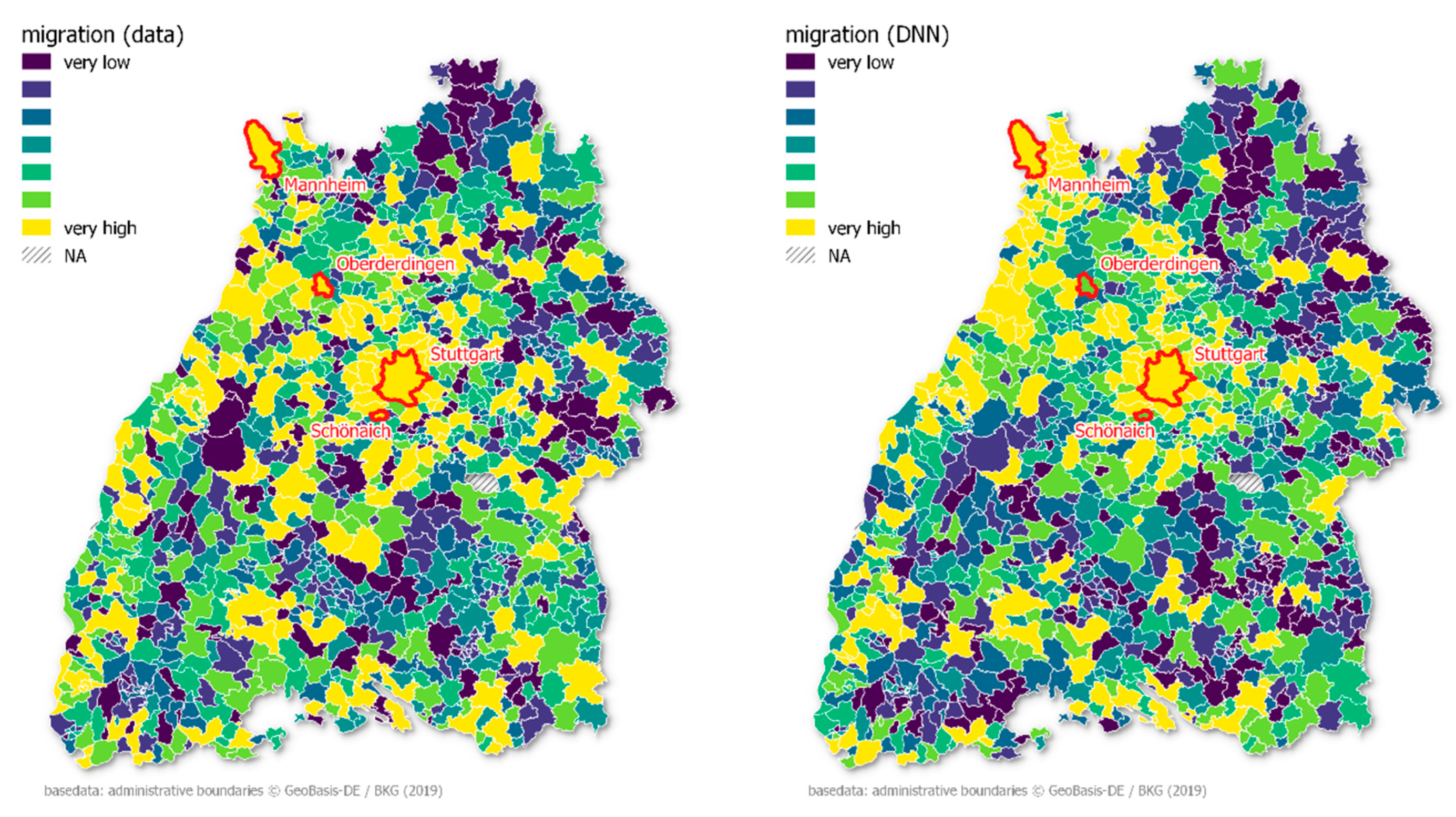
The balance between emigration and immigration and overall spatial attractiveness of a municipality was the third best model. The river Rhine below Freiburg is a highly attractive region after the metropolitan regions of Stuttgart and Karlsruhe (Figure 6).
The Train system is again important for the model, as already observed in the model for the residents. As in the previous model of the elderly population, the dimensions of Nature recreation and Infrastructure are of permutational importance (Table 6). These are followed by the Metropolitan and Industrial area. Similar to the number of residents, the model fails to explain outliers in this category, namely, the cities of Stuttgart and Mannheim. By contrast, the model performs excellently for Schönaich and Oberderdingen.
4. Discussion
Developing dynamic socio-economic indicators for measuring development or vulnerability and describing complex phenomena remains a challenge despite the overall growth of data availability. In this study, socio-economic indicators for residents, unemployment, elderly, and migration are spatially predicted from OSM data with machine learning algorithms.
4.1. Residents
The DNN model, which performed best for all options, predicted the number of residents with the feature elements from the categories Train systems, Infrastructure, Shopping, and Cultural rurality. Stuttgart, the largest urban agglomeration in the dataset, was misrepresented, showing the struggle of the model to differentiate outliers from extreme values. This shows the problem of reproducing extreme values with machine learning algorithms and the need for complete datasets. As these models produce more reliable estimates the more complete the data are, they show weaknesses for the extreme values in narrow datasets when detection of outliers and differentiation from extreme values is unreliable due to similarity in numbers.
4.2. Unemployment
Looking deeper into the modeling of the unemployment rates, we saw that the model largely explained unemployment with Tourism, Natural sights, and Historic rurality. This shows the direct link of natural and cultural heritage to tourism and employment rates in the Black Forest region. If not protected, cultural and natural assets can be shown to have large negative impacts on employment rates.
Unemployment is, however, overestimated for the metropolitan regions. This can be explained by several facts. Firstly, the model explains employment with Natural and Cultural heritage, which does not reproduce urban agglomerations where the labor market is close to full employment. Furthermore, a specific characteristic of the federal state is a highly decentralized economy with hidden champions on the countryside providing excellent jobs in rural areas but also struggling to get highly qualified employees. The study on the region of Stuttgart revealed similar trends [18]. To further investigate and not only predict unemployment, the normalization of the data needs exploration, which is in line with preceding studies to adjust for OSM spatial diversity in contribution [17,18]. Furthermore, training the model with a larger dataset incorporating more large cities, thus stabilizing the extreme value distribution, might resolve this issue for the machine learning algorithms.
Furthermore, the model showed errors in predicting unemployment for Schluchsee and Heidenheim an der Brenz. The municipality of Schluchsee profits from its large number of recreational options around the lake. A variety of recreational options, such as hiking, diving, sailing, and swimming, and in winter, skiing, makes it a popular tourist destination. Therefore, the better performance of the municipality compared to the region partially explains the higher MAE. In Heidenheim, unemployment increased by 12.6% within the last year, far more than in the rest of the region [42].
Nonetheless, a major strength of the methodology presented is revealed by displaying this spatial assessment of connections. By focusing on the distillation of very complex interrelations, regional decision-makers can see the complex relations between the protection of cultural and natural heritage and employment in the tourism industry displayed on the map. This method has the potential to be developed in further research to extract unknown connections, combining target-oriented regional management with success control.
4.3. Elderly
For elderly people, the DNN model focuses strongly on nature-related variables and care facilities. Looking deeper into the third indicator of elderly people, the model performance of the municipality Untermarchtal stands out. Due to the unique setting of Untermarchtal, with its active monastery, including a special care home and only 893 inhabitants, the model underestimates the high proportion of elderly people. Similar to the findings of [22], rural sites can be dominated by a single economic player, and this situation is not well represented by the models. It could also be helpful to screen the municipalities with very low MAEs, such as Schönaich, Oberderdingen, Wittighausen, and Kappelrodeck, which are well represented due to the median values.
Interestingly, the third explanatory variable was mobility. Relating elderly to public transport, the strength of the method provided here can be seen. In the OSM dataset, information on infrastructure, nature, and cultural heritage, but also mobility and connectivity, can be assessed in depth, gaining knowledge about new relations and connections with machine learning algorithms. This study results in spatial information about the dependence of elderly people on reliable public transport. As such, in combination with ongoing demographic change, a decision-maker would now have the possibility to assess future demand for mobility capacity needs and target the development of specific public transport for the elderly according to the distilled spatial distribution.
4.4. Migration
In addition to the cross-cutting dimension, each indicator is specified by explicit dimensions. Migration can be described by Infrastructure, Economic, Provision of services, and Natural characteristics.
In line with residents and unemployment, the DNN model also struggled to predict extreme values for migration balance. The problem was aggravated in cases where extreme values were part of the test data. Predicting the migration balance, the two largest cities of Baden-Württemberg, Stuttgart and Karlsruhe, were not well reproduced.
4.5. Model Comparison
When deepening the analysis of the different model performances, we saw that DNN performs most reliably. The two machine learning algorithm MAEs were much closer to one another. Still, DNN was better than or equal to RF in all four cases. This is in line with current research, as deep neural networks have outperformed many models in previous studies [43,44,45,46,47,48,49]. Despite the slightly worse performance of RF, it is worth mentioning that the DNN required substantial model configuration, without which it performed much worse than both other methods. Moreover, RF is easier to communicate and understand. The feature importance of the RF was implemented within the approach. Here, DNN is often seen as a black box, making it difficult to understand driving factors [49]. In addition, the RF proved to be more robust and much easier to execute. Without extensive training, we could observe a deterioration in the DNN model performance, as a sensitivity to the training and test data selection became apparent. RF produced robust and less sensitive results compared to random sampling. The computational needs for RF were also much lower than for DNN. Hence, in cases where maximal model performance is needed, DNN is the model of choice, whereas for data mining and understanding, RF often seems to perform quite well.
In increasing order, starting with the lowest MAE of the DNN, the indicator population was best predicted, followed by migration, elderly, and unemployment. Although DNN had superior predictive power, the model performed badly on the outliers and in the extreme values. This could especially be seen when reproducing the number of residents on a regional scale, as estimations for residents in the larger cities were worse. This was mainly the case for Stuttgart and for Karlsruhe. This might, however, be resolved by deepening the research with larger datasets incorporating more large cities, so that the extreme value distribution is stabilized and produces more reliable estimates.
4.6. Challenges
An important part of socio-economic indicators is their explanatory power of unusual phenomena or in extreme situations. Machine learning, and especially DNN, is often seen as a black box, which limits its acceptance and applicability [50]. Nonetheless, the PFI is a very condensed way of interpreting the global feature importance. As the approach is linked to the error of the model, it is only possible to perform with access to the outcome and not for the assessment of a standalone model [51]. By leaving out different explanatory variables, the assessment of their contribution to the overall outcome distills the interconnections of social indicators and spatial attributes, which is key in understanding regional development issues and helps in making target-oriented decisions.
Furthermore, one major challenge that kept coming up in all the indicators was the representation of extreme values. As such, it could be shown in this study that the representation of extreme value distribution is, as is in any modeling effort, one major flaw in the methodology. This being an interwoven problem of the availability of wide-ranging datasets for model training, the complex process of differentiating between outliers and extreme values, and the simultaneous training of models to represent normal distributions and extreme value distributions.
An important common constraint of OSM data is the spatially unbalanced contribution and, hence, the variations in spatial coverage and density of information, especially on a global level. Germany, and especially the selected study region, is among the regions with a comparatively high number of contributors and a high coverage of information, represented, for example, by a completeness index of above 50% in 2016 for Germany [52]. Nevertheless, the completeness within the country still shows a disparity between rural areas and urban regions regarding data coverage and quality [53,54], which could limit the explanatory power of the model results in this study. Therefore, it would be interesting to see if certain thresholds could be established for regions with lower coverage or if the absence of OSM data themselves can be used in this context as a predictor. Another shortcoming is that the handling of the method is not user-friendly. Machine learning techniques remain difficult to handle and require a statistical and analytical skillset. Furthermore, the management of the OSM data structure within the model is not very intuitive which, all in all, makes the approach difficult to be used by decision makers. Nevertheless, we have succeeded in showing that OSM data sets contain a great deal of knowledge about socio-economic realities, and that these can be extracted with machine learning. It is not insignificant that these indicators can be represented spatially in map form, which increases their contribution to decision-making.
4.7. Future Research
After having tested the method in the small-scale region of Stuttgart, we further developed the approach. As a compromise between computational resources, data handling, and model complexity, the regional scale was chosen. In further research, the potential at a global scale and transferability of models between regions should be assessed, given the potentially high impact on the results due to different levels of completeness of OSM data and/or the use of different (local) tagging guidelines. In line with a larger dataset, emphasis should be put on better consideration of extreme values. Often decision makers are mainly interested in special cases, i.e., extreme values. Further efforts are needed to be able to provide stable answers to these complex questions at the outer ends of the dataset.
5. Conclusions
Living in a globally interwoven world, rarely is any problem restricted to one singular specific point in space and time. As such, the big challenges of global change and, subsequently, resilience, vulnerability, and sustainability that we are facing are not stationary.
In this light, first understanding and later monitoring multifaceted phenomena demands a global temporal interdisciplinary source of data. OSM is a valuable source of data, and machine learning provides the means of deducing interdisciplinary indicators. OSM documents the physical manifestation of human activities, and these data can be used to perform socio-economic analyses by means of machine learning. Neural networks have succeeded in terms of model performance compared to Random Forest. Here we have shown the attractiveness of this untapped potential for knowledge generation by combining machine and deep learning algorithms with OSM for developing socio-economic indicators. The evaluation provided encouraging insights into the manifestation of socio-economic attributes in OSM data. The approach we developed exposes several advantages, but also several issues that need more consideration.
To fully exploit the opportunities of OSM in terms of spatial coverage, personal computers reach their limitations in data wrangling. Further exploration is required into global predictors and the transferability of models across regions or countries. Additional temporal analyses might further improve the performance of models and their predictive power and help to deduce the most relevant predictors.
Author Contributions
Conceptualization: Daniel Feldmeyer.; data curation: Holger Sauter. and Daniel Feldmeyer; methodology: Daniel Feldmeyer; writing—original draft: Holger Sauter; Daniel Feldmeyer and Claude Meisch; writing—review and editing: Daniel Feldmeyer, Claude Meisch, Holger Sauter and Joern Birkmann. All authors have read and agreed to the published version of the manuscript.
Funding
This research received no external funding.
Conflicts of Interest
The authors declare no conflict of interest.
Data & Workflow
https://github.com/danielfeldmeyer/OSM-indicator (will be provided upon completion of PhD).
Appendix A. Predictor Related Tags
| Predictor | Tags (Highest Loadings) |
| Nature recreation | landuse_forest; route_bycicle; operator_Baden-Würtemberg |
| Infrastructure | Highway_traffic_signals; route_train; highway_crossing_railway_rail |
| Train System | Route_tracks; railway_rail; operator_DB Netz; route_railway |
| Natural sights | Tourism_viewpoint; width_1; boundary_natural; natural_mountain_range; food_yes |
| Tourism | Shop_books; tourism_museum; historic_castle; tourism_hotel |
| Metropolitan | Route_bus; oneway_yes; highway_milestone |
| Suburban | Building_garage; route_power; landuse_recreation_ground; waterway_drain; power_line |
| Nature | Natural_mountain_range; place_region; boundary_natural; route_ski; amenity_waste_basket |
| Historic rural | Highway_living_street; historic_archeological; man_made_bridge; operator_DHL |
| Industrial | Landuse_idustrial; sport_multi; surface_gravel; leisure_track |
| Rurality | power_cable; place_hamlet; bicycle_use_sidepath; building_public |
| Social care | Building_kindergarten; amenity_nursing_home; leisure_track; |
| Nursing home | amenity_nursing_home, width_10; denomination_new_apostolic |
| Shopping & culture | Shop_deli; amenity_arts_center; shop_beverages |
References
- Measuring Vulnerability to Natural Hazards. Towards Disaster Resilient Societies, 2nd ed.; Birkmann, J., Ed.; United Nations University Press: Tokyo, Japan; New York, NY, USA, 2013; ISBN 9789280871715. [Google Scholar]
- Sorg, L.; Medina, N.; Feldmeyer, D.; Sanchez, A.; Vojinovic, Z.; Birkmann, J.; Marchese, A. Capturing the multifaceted phenomena of socioeconomic vulnerability. Nat. Hazards 2018, 92, 257–282. [Google Scholar] [CrossRef] [Green Version]
- Jamshed, A.; Rana, I.A.; Mirza, U.M.; Birkmann, J. Assessing relationship between vulnerability and capacity: An empirical study on rural flooding in Pakistan. Int. J. Disaster Risk Reduct. 2019, 36, 101109. [Google Scholar] [CrossRef]
- Cutter, S.L.; Finch, C. Temporal and spatial changes in social vulnerability to natural hazards. Proc. Natl. Acad. Sci. USA 2008, 105, 2301–2306. [Google Scholar] [CrossRef] [PubMed] [Green Version]
- Kotsev, A.; Minghini, M.; Tomas, R.; Cetl, V.; Lutz, M. From Spatial Data Infrastructures to Data Spaces—A Technological Perspective on the Evolution of European SDIs. ISPRS Int. J. Geo-Inf. 2020, 9, 176. [Google Scholar] [CrossRef] [Green Version]
- Feldmeyer, D.; Wilden, D.; Kind, C.; Kaiser, T.; Goldschmidt, R.; Diller, C.; Birkmann, J. Indicators for Monitoring Urban Climate Change Resilience and Adaptation. Sustainability 2019, 11, 2931. [Google Scholar] [CrossRef] [Green Version]
- Schaefer, M.; Thinh, N.X.; Greiving, S. How Can Climate Resilience Be Measured and Visualized? Assessing a Vague Concept Using GIS-Based Fuzzy Logic. Sustainability 2020, 12, 635. [Google Scholar] [CrossRef] [Green Version]
- Leinenkugel, P.; Deck, R.; Huth, J.; Ottinger, M.; Mack, B. The Potential of Open Geodata for Automated Large-Scale Land Use and Land Cover Classification. Remote Sens. 2019, 11, 2249. [Google Scholar] [CrossRef] [Green Version]
- Mishra, N.B.; Crews, K.A. Mapping vegetation morphology types in a dry savanna ecosystem: Integrating hierarchical object-based image analysis with Random Forest. Int. J. Remote Sens. 2014, 35, 1175–1198. [Google Scholar] [CrossRef]
- Blomdahl, E.M.; Thompson, C.M.; Kane, J.R.; van Kane, R.; Churchill, D.; Moskal, L.M.; Lutz, J.A. Forest structure predictive of fisher (Pekania pennanti) dens exists in recently burned forest in Yosemite, California, USA. For. Ecol. Manag. 2019, 444, 174–186. [Google Scholar] [CrossRef]
- Hütt, C.; Waldhoff, G. Multi-data approach for crop classification using multitemporal, dual-polarimetric TerraSAR-X data, and official geodata. Eur. J. Remote Sens. 2018, 51, 62–74. [Google Scholar] [CrossRef]
- Deville, P.; Linard, C.; Martin, S.; Gilbert, M.; Stevens, F.R.; Gaughan, A.E.; Blondel, V.D.; Tatem, A.J. Dynamic population mapping using mobile phone data. Proc. Natl. Acad. Sci. USA 2014, 111, 15888–15893. [Google Scholar] [CrossRef] [PubMed] [Green Version]
- Sheikhian, H.; Delavar, M.R.; Stein, A. A GIS-based multi-criteria seismic vulnerability assessment using the integration of granular computing rule extraction and artificial neural networks. Trans. GIS 2017, 21, 1237–1259. [Google Scholar] [CrossRef]
- Wlodarczyk-Sielicka, M.; Lubczonek, J. The Use of an Artificial Neural Network to Process Hydrographic Big Data during Surface Modeling. Computers 2019, 8, 26. [Google Scholar] [CrossRef] [Green Version]
- Kim, D.-E.; Gourbesville, P.; Liong, S.-Y. Overcoming data scarcity in flood hazard assessment using remote sensing and artificial neural network. Smart Water 2019, 4, 183. [Google Scholar] [CrossRef]
- Cillis, G.; Lay-Ekuakille, A.; Telesca, V.; Statuto, D.; Picuno, P. Analysis of the Evolution of a Rural Landscape by Combining SAR Geodata with GIS Techniques. In Innovative Biosystems Engineering for Sustainable Agriculture, Forestry and Food Production; Coppola, A., Di Renzo, G.C., Altieri, G., D’Antonio, P., Eds.; Springer International Publishing: Basel, Switzerland, 2020; pp. 255–263. ISBN 978-3-030-39298-7. [Google Scholar]
- Feldmeyer, D.; Sauter, H.; Birkmann, J. An open risk index with learning indicators from OSM-tags, developed by machine learning and trained with the WorldRiskIndex. Int. Arch. Photogramm. Remote Sens. Spat. Inf. Sci. 2019, XLII-4/W14, 37–44. [Google Scholar] [CrossRef] [Green Version]
- Sauter, H.; Feldmeyer, D.; Birkmann, J. Exploratory study of urban resilience in the region of Stuttgart based on OpenStreetMap and literature resilience indicators. Int. Arch. Photogramm. Remote Sens. Spat. Inf. Sci. 2019, XLII-4/W14, 213–220. [Google Scholar] [CrossRef] [Green Version]
- Statistisches Bundesamt. Bevölkerungsdichte (Einwohner je km²) in Deutschland Nach Bundesländern zum 31 December 2018. Available online: https://de.statista.com/statistik/daten/studie/1242/umfrage/bevoelkerungsdichte-in-deutschland-nach-bundeslaendern/ (accessed on 5 October 2019).
- GfK. Kaufkraft Je Einwohner Nach Bundesländern Im Jahr 2019 Laut GfK-Kaufkraftstudie. Available online: https://de.statista.com/statistik/daten/studie/168591/umfrage/kaufkraft-nach-bundeslaendern/ (accessed on 4 December 2019).
- Bundesagentur für Arbeit. Monatliche Arbeitslosenquote in Baden-Württemberg von November 2018 bis November 2019. Available online: https://de.statista.com/statistik/daten/studie/155318/umfrage/arbeitslosenquote-in-baden-wuerttemberg/ (accessed on 4 December 2019).
- Statistisches Landesamt. Baden-Württemberg: Bevölkerung im Schnitt 43,5 Jahre alt: Jüngste Einwohner in Riedhausen (Landkreis Ravensburg), älteste in Ibach (Landkreis Waldshut). Available online: https://www.statistik-bw.de/Presse/Pressemitteilungen/2019211 (accessed on 4 December 2019).
- Statistisches Landesamt. 294,000 Hochbetagte in Baden-Württemberg Zahl Der 85-Jährigen Und Älteren Hat Sich Seit 1970 Versechsfacht–Baden-Baden Mit Höchstem Anteil an Der Bevölkerung. Available online: https://www.statistik-bw.de/Presse/Pressemitteilungen/2019254 (accessed on 2 October 2019).
- Cutter, S.L.; Burton, C.G.; Emrich, C.T. Disaster Resilience Indicators for Benchmarking Baseline Conditions. J. Homel. Secur. Emerg. Manag. 2010, 7. [Google Scholar] [CrossRef]
- Cutter, S.L. The landscape of disaster resilience indicators in the USA. Nat. Hazards 2015, 80, 741–758. [Google Scholar] [CrossRef]
- UN. Global Indicator Framework for the Sustainable Development Goalsand Targets of the 2030 Agenda for Sustainable Development: Sustainable Development Goal Indicators should be Disaggregated, where Relevant, by Income, Sex, Age, Race, Ethnicity, Migratory Status, Disability and Geographic Location, or Other Characteristics, in Accordance with the Fundamental Principles of Official Statistics. Available online: https://unstats.un.org/sdgs/indicators/Global%20Indicator%20Framework%20after%202019%20refinement_Eng.pdf (accessed on 4 December 2019).
- OpenStreetMap Contributors. Planet Dump. Available online: https://www.openstreetmap.org (accessed on 2 October 2019).
- OpenStreetMap-Deutschland. FAQs: Was Ist OpenStreetMap? Available online: https://www.openstreetmap.de/faq.html#was_ist_osm (accessed on 9 April 2020).
- OpenStreetMap. Stats. Available online: https://wiki.openstreetmap.org/wiki/Stats (accessed on 9 April 2020).
- RStudio: Integrated Development for R [Computer Software]; RStudio, Inc.: Boston, MA, USA, 2016; Available online: http://www.rstudio.com/ (accessed on 17 April 2020).
- R Core Team. A Language and Environment for Statistical Computing; R Foundation for Statistical Computing: Vienna, Austria, 2019; ISBN 9783900051075. [Google Scholar]
- Wickham, H.; Henry, L. Tidyr: Tidy Messy Data. R Package Version 1.0.0. Available online: https://CRAN.R-project.org/package=tidyr (accessed on 5 November 2019).
- Wickham, H.; Francois, R.; Henry, L.; Müller, K.; RStudio. Dplyr: A Grammar of Data Manipulation. R Package Version 1.0.2. Available online: https://CRAN.R-project.org/package=dplyr (accessed on 5 November 2019).
- Wickham, H.; Oom, J.; Müller, K.; RStudio; R Consortium; Tomoaki, N. RPostgres ‘Rcpp’ Interface to ‘PostgreSQL’. R Package Version 1.2.0. Available online: https://CRAN.R-project.org/package=RPostgres (accessed on 5 November 2019).
- Wickham, H. Reshaping Data with the reshape Package. J. Stat. Softw. 2007, 21, 1–20. [Google Scholar] [CrossRef]
- Wickham, H.; Bryan, J. Readxl: Read Excel Files. R Package Version 1.3.1. Available online: https://CRAN.R-project.org/package=readxl (accessed on 5 November 2019).
- Kuhn, M.; Wing, J.; Weston, S.; Williams, A.; Keefer, A.; Engelhardt, A.; Cooper, T.; Mayer, Z.; Kenkel, B.; R Core Team; et al. Caret: Classification and Regression Training. R Package Version 6.0-86. Available online: https://CRAN.R-project.org/package=caret (accessed on 5 November 2019).
- Liaw, A.; Wiener, M. RandomForest: Breiman and Cutler’s Random Forests for Classification and Regression. R Package Version 4.6-14. Available online: https://CRAN.R-project.org/package=randomForest (accessed on 5 November 2019).
- Allaire, J.J.; Chollet, F. Keras: R Interface to ‘Keras’. R Package Version 2.3.0.0. Available online: https://CRAN.R-project.org/package=keras (accessed on 5 November 2019).
- Breiman, L. Random Forests. Mach. Learn. 2001, 45, 5–32. [Google Scholar] [CrossRef] [Green Version]
- Fisher, A.; Rudin, C.; Dominici, F. All Models are Wrong, but Many are Useful: Learning a Variable’s Importance by Studying an Entire Class of Prediction Models Simultaneously. J. Mach. Learn. Res. 2019, 20, 1–81. [Google Scholar]
- Swp. Arbeitslose in Ostwürttemberg. Available online: https://www.swp.de/suedwesten/staedte/gaildorf/ostwuerttemberg-arbeitslose-arbeitsmarkt-agenturfuerarbeit-statistik-38704793.html (accessed on 12 November 2019).
- Miguel-Hurtado, O.; Guest, R.; Stevenage, S.V.; Neil, G.J.; Black, S. Comparing Machine Learning Classifiers and Linear/Logistic Regression to Explore the Relationship between Hand Dimensions and Demographic Characteristics. PLoS ONE 2016, 11, e0165521. [Google Scholar] [CrossRef] [PubMed]
- Belgiu, M.; Drăguţ, L. Random forest in remote sensing: A review of applications and future directions. ISPRS J. Photogramm. Remote Sens. 2016, 114, 24–31. [Google Scholar] [CrossRef]
- Berk, R. Machine Learning Risk Assessments in Criminal Justice Settings; Springer International Publishing: Cham, Switzerland, 2019; ISBN 9783030022730. [Google Scholar]
- Witten, I.H.; Frank, E.; Hall, M.A.; Pal, C.J. Data mining. In Practical Machine Learning Tools and Techniques, 4th ed.; Morgan Kaufmann Publisher: Cambridge, MA, USA, 2017; ISBN 978-0-12-374856-0. [Google Scholar]
- E Sousa, L.R.; Miranda, T.; E Sousa, R.L.; Tinoco, J. The Use of Data Mining Techniques in Rockburst Risk Assessment. Engineering 2017, 3, 552–558. [Google Scholar] [CrossRef]
- Xu, P.; Shi, S.; Chu, X. Performance Evaluation of Deep Learning Tools in Docker Containers. In Proceedings of the 2017 3rd International Conference, Chengdu, China, 10–11 August 2017; pp. 395–403. [Google Scholar]
- Engchuan, W.; Dimopoulos, A.C.; Tyrovolas, S.; Caballero, F.F.; Sanchez-Niubo, A.; Arndt, H.; Ayuso-Mateos, J.L.; Haro, J.M.; Chatterji, S.; Panagiotakos, D.B. Sociodemographic Indicators of Health Status Using a Machine Learning Approach and Data from the English Longitudinal Study of Aging (ELSA). Med. Sci. Monit. 2019, 25, 1994–2001. [Google Scholar] [CrossRef] [Green Version]
- Ribeiro, M. Visualizing ML Models with LIME. Available online: https://uc-r.github.io/lime (accessed on 4 December 2019).
- Fioruzi, H.O. End-to-End Implementation of Deep Learning in R Using Keras. Available online: https://rstudio-pubs-static.s3.amazonaws.com/452498_2bb5b64288b94710a86982c3f70bb483.html#4_model_interpretabilitydiagnosis (accessed on 5 November 2019).
- Arsanjani, J.; Fonte, C. On the Contribution of Volunteered Geographic Information to Land Monitoring Efforts. In European Handbook of Crowdsourced Geographic Information; Capineri, C., Haklay, M., Huang, H., Antoniou, V., Kettunen, J., Ostermann, F., Purves, R., Eds.; Ubiquity Press: London, UK, 2016; pp. 269–284. Available online: www.jstor.org/stable/j.ctv3t5r09.24 (accessed on 17 April 2020).
- Zielstra, D.; Zipf, A. A comparative study of proprietary geodata and volunteered geographic information for Germany. In Proceedings of the 13th AGILE International Conference on Geographic Information Science, Guimarães, Portugal, 11–14 May 2010. [Google Scholar]
- Haklay, M. How good is volunteered geographical information? A comparative study of OpenStreetMap and ordnance survey datasets. Environ. Plan. B Plan. Des. 2010, 37, 682–703. [Google Scholar] [CrossRef] [Green Version]
Figure 1.
Overall workflow of the analysis conducted.

Figure 2.
Map of study area.

Figure 3.
Map showing the normalized resident values (left) and predicted values (right) of the municipalities in Baden-Württemberg.
Figure 3.
Map showing the normalized resident values (left) and predicted values (right) of the municipalities in Baden-Württemberg.

Figure 4.
Map showing the normalized unemployment values (left) and predicted values (right) of the municipalities in Baden-Württemberg.
Figure 4.
Map showing the normalized unemployment values (left) and predicted values (right) of the municipalities in Baden-Württemberg.

Figure 5.
Map showing the normalized proportion of elderly people (left) and predicted values (right) of the municipalities in Baden-Württemberg.
Figure 5.
Map showing the normalized proportion of elderly people (left) and predicted values (right) of the municipalities in Baden-Württemberg.

Figure 6.
Map showing the normalized migration balance (left) and predicted values (right) of the municipalities in Baden-Württemberg.
Figure 6.
Map showing the normalized migration balance (left) and predicted values (right) of the municipalities in Baden-Württemberg.


Table 1.
Data table of spatial attributes per municipality.
| Name | Key_Value [Count/Municipality] | Key_Value [km/Municipality] | Key_Value [km2/Municipality] |
|---|---|---|---|
| Municipality 1 | Value | Value | Value |
| Municipality 2 | Value | Value | Value |
Table 2.
Mean absolute error of the models for the indicators. RP, random prediction; DNN, deep neural networks; LR, linear regression; RF, random forest.
Table 2.
Mean absolute error of the models for the indicators. RP, random prediction; DNN, deep neural networks; LR, linear regression; RF, random forest.
| Dataset | RP | LR | RF | DNN |
|---|---|---|---|---|
| Residents | 0.489 | 0.049 | 0.038 | 0.021 |
| Unemployment | 0.280 | 0.119 | 0.099 | 0.095 |
| Elderly | 0.311 | 0.090 | 0.074 | 0.071 |
| Migration | 0.405 | 0.041 | 0.035 | 0.025 |
Table 3.
Most important predictors of residents.
| PFI Rank | Predictor |
|---|---|
| 1 | Train system |
| 2 | Infrastructure |
| 3 | Shopping and culture |
| 4 | Rurality |
Table 4.
Most important predictors of unemployment.
| PFI Rank | Predictor |
|---|---|
| 1 | Tourism |
| 2 | Natural sights |
| 3 | Historic rural |
| 4 | Train system |
| 5 | Social care |
Table 5.
Most important predictors of the elderly.
| PFI Rank | Predictor |
|---|---|
| 1 | Nature recreation |
| 2 | Infrastructure |
| 3 | Nature |
| 4 | Suburban |
| 5 | Nursing home |
Table 6.
The most important predictors of migration.
| PFI Rank | Predictor |
|---|---|
| 1 | Train system |
| 2 | Nature recreation |
| 3 | Infrastructure |
| 4 | Metropolitan |
| 5 | Industrial |
© 2020 by the authors. Licensee MDPI, Basel, Switzerland. This article is an open access article distributed under the terms and conditions of the Creative Commons Attribution (CC BY) license (http://creativecommons.org/licenses/by/4.0/).
Share and Cite
MDPI and ACS Style
Feldmeyer, D.; Meisch, C.; Sauter, H.; Birkmann, J. Using OpenStreetMap Data and Machine Learning to Generate Socio-Economic Indicators. ISPRS Int. J. Geo-Inf. 2020, 9, 498. https://doi.org/10.3390/ijgi9090498
AMA Style
Feldmeyer D, Meisch C, Sauter H, Birkmann J. Using OpenStreetMap Data and Machine Learning to Generate Socio-Economic Indicators. ISPRS International Journal of Geo-Information. 2020; 9(9):498. https://doi.org/10.3390/ijgi9090498
Chicago/Turabian StyleFeldmeyer, Daniel, Claude Meisch, Holger Sauter, and Joern Birkmann. 2020. "Using OpenStreetMap Data and Machine Learning to Generate Socio-Economic Indicators" ISPRS International Journal of Geo-Information 9, no. 9: 498. https://doi.org/10.3390/ijgi9090498
Note that from the first issue of 2016, this journal uses article numbers instead of page numbers. See further details here.