Mining Type-β Co-Location Patterns on Closeness Centrality in Spatial Data Sets

Abstract

A co-location pattern is a set of spatial features whose instances are frequently correlated to each other in space. Its mining models always consist of two essential steps. One step is to generate neighbor relationships between spatial instances, and another step is to check the prevalence of candidate patterns on the clique, star or Delaunay triangulation relationships. At least three major issues are addressed in this paper. First, since different spatial regions, different distribution densities, it is difficult to set appropriate parameters to generate ideal neighbor relationships. Second, the clique relationship and the others are so strongly rigid that the users’ personal interests are suppressed; some interesting patterns are neglected without increasing redundancy. Third, the different strength of correlations among instances are neglected in prevalence calculation. It causes correlations among features to be undifferentiated. Accordingly, the main work of this paper includes: (1) The neighbor relationship generation can be improved on the idea that the distances between an instance and any of its neighbors are not remarkably different. (2) The type-$\beta$ co-location pattern is defined and checked based on a co-occurrence where the closeness centrality of each instance is not less than a given threshold $\beta$. (3) Since the closeness centrality carries strength of correlations among instances, the strength of the correlations between a feature and the other ones in a type-$\beta$ co-location pattern can be evaluated with prevalence calculation. Finally, experiments on synthetic and real-world spatial data sets are used to assess the effectiveness and efficiency of our works. The results show that fewer spatial neighbor relationships are generated, and more interesting patterns can be discovered by flexibly adjusting $\beta$ according to the user’s preferences.

1. Introduction

Spatial data mining has reached its pinnacle with the advancement of data collecting and processing technology. One of the most important research interests in this domain is co-location pattern mining [1]. For co-location pattern mining in spatial data sets, a spatial feature is a label of some objects (e.g., the clover). Furthermore, an instance is a feature’s object with location information. A co-location pattern is a spatial feature set whose instances are frequently located together in a geographic space [2]. The co-location pattern {the clover, the wasp, the vole, the cat, the cow}, for example, reveals that the instances of the spatial features in this pattern make a healthy livestock ecological system [3]. Co-location pattern mining is widely employed in domains such as ecological protection, public hygiene, urban planning, ad distribution, and so on because co-location patterns may disclose the co-occurrence of spatial features [4].

Generally, there are two major steps to mine co-location patterns in the traditional models.

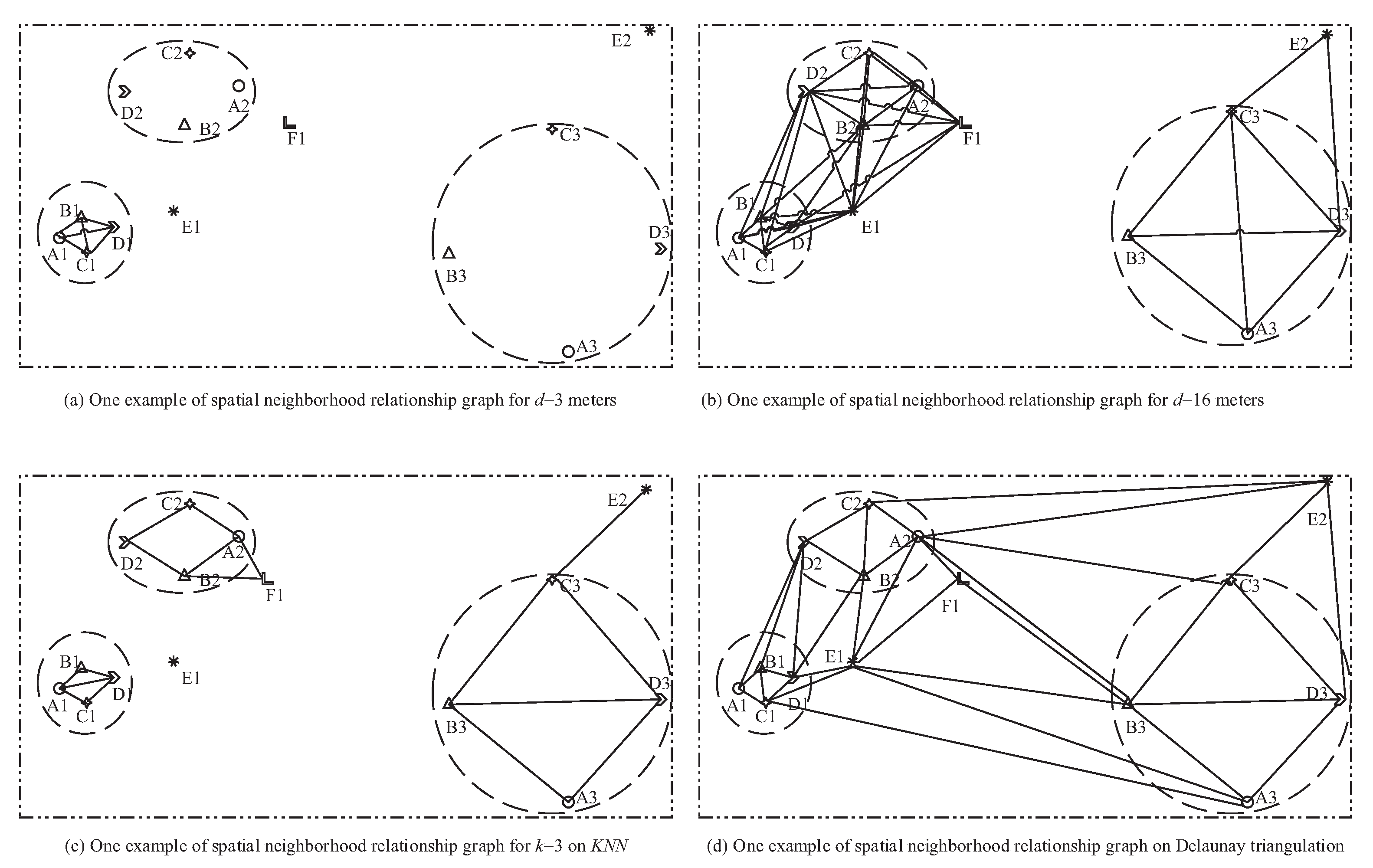
One step is to generate spatial neighbor relationships in instances from the given spatial data sets. Neighbor relationships (i.e., spatial proximity) follow Tobler’s First Law of geography: Everything is related to everything else but nearby things are more related than distant things. However, Goodhild’s Second Law of Geography claims that geographic variables exhibit uncontrolled variance. That is to say, the ideal neighbors are not only correlated to distances (the First Law) but also related to regional distribution densities (the Second Law). For example, assuming A1 and D1 are neighbors in Figure 1, so are A1 and B1. Although the distance between A3 and B3 is similar to the one between B2 and D1, there is a stronger correlation between A3 and B3 than between B2 and D1 because of their different regional distribution densities.

Another step is to check the prevalence of candidate patterns on the spatial neighbor relationships. The instances of each pattern (i.e., checklists for prevalence) should be on the co-occurrence such as the clique [5], star [6], or triangle-based relationships [7]. Generally, the higher the ratio of co-occurrences, the higher the prevalence of the pattern. For example, {A2, B2, C2, D2} obviously supports the prevalence of {A, B, C, D}, even if it is not a clique or star in Figure 1c.

1.1. Motivation

Although many scholars have been engaged in relevant research, at least three problems remain.

• It is difficult to build a model to generate neighbor relationships to adapt data sets with different distribution densities. To obtain neighbor relationships satisfied to densities, many scholars have proposed different solutions. Figure 1 shows some representative approaches on distance thresholds, such as KNN and the Delaunay triangulation. For example, it is intuitive that A1 and B1 are neighbors of each other in a dense region, and so are A3 and B3 in a sparse zone. On the contrary, it is intuitive that B2 and D1 are not neighbors of each other while B3 and D3 are. As a result, it is not friendly to determine an optimal distance threshold to generate neighbor relationships even for experimental users because (a) too small of a distance threshold may underestimate the prevalence of patterns in sparse regions (e.g., Figure 1a) while (b) a too big one may overestimate the prevalence of patterns in dense zones (e.g., Figure 1b). For example, A1 and D1 should not be considered to be neighbors of each other, while D1 and E1 can be considered to be neighbors of each other in Figure 1d. Furthermore, neighbor relationships in different density areas can overlap but not split. This is the biggest difference between co-location pattern mining and transaction-based association analysis. For example, D1 and E1 can be neighbors of each other in a dense zone, and so can B2 and E1 in a sparse region. Thus, this statement is not friendly to classical clustering.
• The instance of a pattern should be a co-occurrence, and then it would be perfect to integrate and extend the traditional co-occurrences such as the clique, star, and so on [8]. For example, {A2, B2, C2, D2} is suggested to not be an instance of {A, B, C, D}, while the instance is based on the clique in Figure 1a. However, the correlation in {A2, B2, C2, D2} is also strong. Furthermore, {A, B, C, D} selectively occurs in other regions of Figure 1. If instances of patterns are based on the clique, {A, B, C, D} can be prevalent only in Figure 1b when the prevalence threshold is 1. This cannot meet the expectation that the features in {A, B, C, D} are strongly correlated. Furthermore, the same users may be interested in patterns with different correlations in different data sets, let alone different users. To obtain expected patterns, users always have to resize either the parameter of neighbor relationships generation or prevalence threshold in traditional co-location pattern mining models. It inevitably leads to redundancy. For example, to obtain {A, B, C, D} in Figure 1, the prevalence threshold should be reduced to 1/3 if the neighbor relationships is as Figure 1a, or the distance threshold should be increased to 16 m such as in Figure 1b when the prevalence threshold is 1.
• Since traditional models check the prevalence of patterns are generally on features’ instance appearance ratios, it inevitably loses instance topology on the spatial neighbor relationships. For example, it can be acknowledged that {B, C, D} is more correlated than {B, D, E} even if the instances of each corresponding feature have appeared in the two patterns with an adaptive definition of pattern instances. The correlation between a feature and the other ones in a pattern can be evaluated from the topology of the pattern’s instances. Understandably, if the instances of a feature in a pattern always have a higher center in the topology, the feature has a stronger correlation with the other features in the pattern than the other ones have. How can the spatial neighbor relationships be transmitted and accumulated to the interesting patterns? This problem needs to be studied urgently. For example, B and C are more likely to be in the center of the topology than A and D in {A, B, C, D} in Figure 1.

1.2. Overall Solution

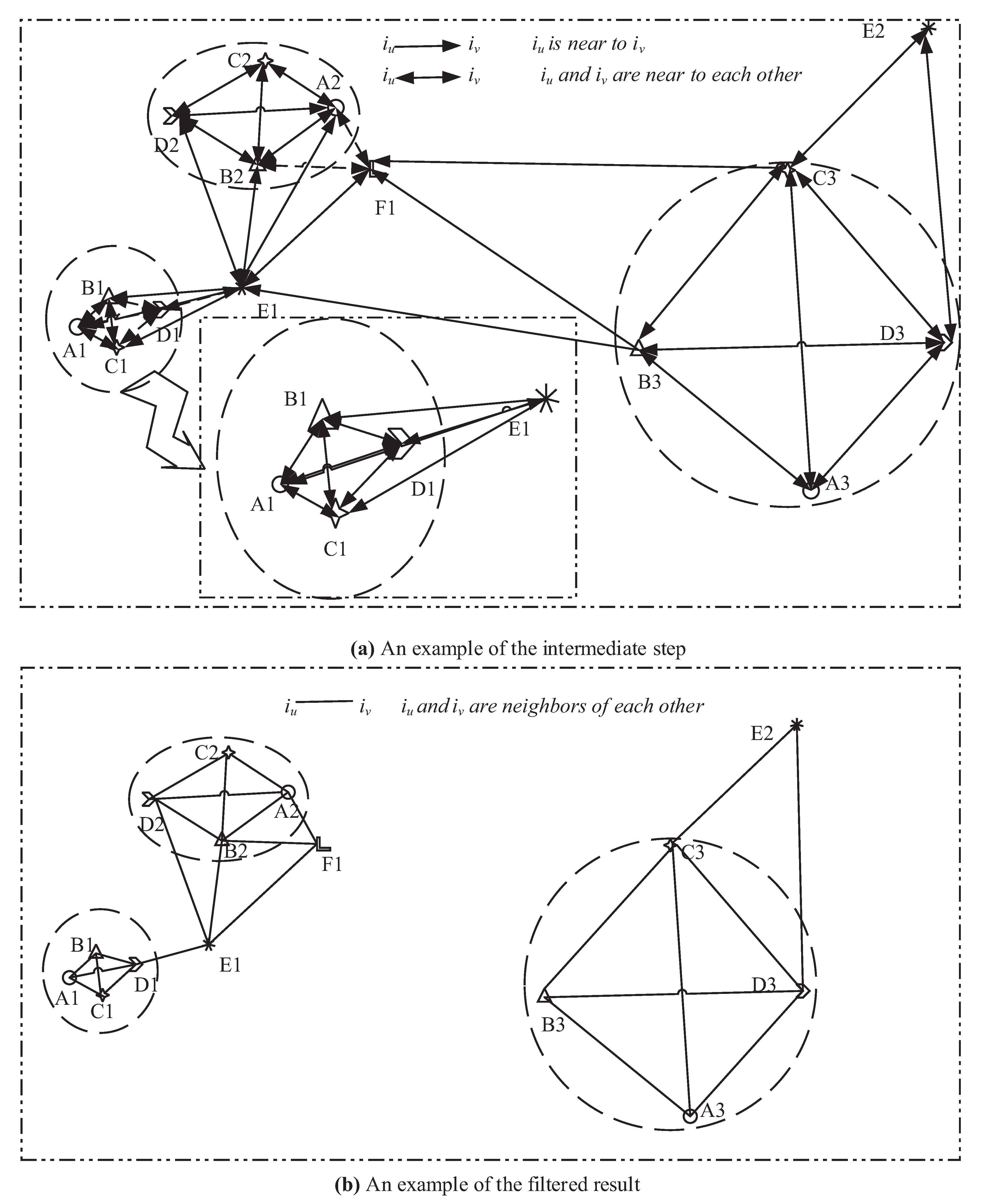
Understandably, distances between any instance and its neighbors tend to be similar but not widely different. For example, B1, C1, and D1 can be considered to be neighbors of A1, but B2 is not because it is intuitively further than B1, C1, and D1 from A1 in Figure 1. Moreover, A2, B2, C2, D2, and E1 can be neighbors of F1, but B3 cannot, because B3 is obviously further than A2, B2, C2, D2, and E1 from F1. Thus, a robust way with a compromise of distance threshold and KNN is proposed to generate a more applicable neighbor relationship set in this paper. For an instance denoted $i_u$, the distance between $i_u$ and its nearest neighbor except itself is denoted $dst$. Given an elastic coefficient $\alpha$ and an instance $i_v$, if the distance between $i_u$ and $i_v$ is not further than $dst\ast \alpha$, $i_v$ can be considered to be a directed neighbor of $i_u$. For example, the distances from A1 to B1, C1, D1, E1, and B2 are, respectively, 3, 3.2, 4.8, 10.7, and 15.7. Therefore, B1, C1, and D1 are considered to be directed neighbors of A1 when $1.6\ge \alpha \le 3.6$. Furthermore, for any pair of instances, if and only if they are directed neighbors of each other, they are mutual neighbors of each other. For example, D1 and E1 are mutual neighbors of each other but A1 and E1 are not, as A1 is a directed neighbor of E1 but not vice versa. A mutual neighbor relationship graph is shown in Figure 2b. It is obvious that a lower $dst$ leads a denser region. On the contrary, a greater $dst$ leads a sparser region. That is to say, the threshold $dst\ast \alpha$ can help neighbor relationship generation be adaptive to region distribution densities.

To measure the prevalence of patterns, their instances should be detected on the neighbor relationships. Scholars tend to define patterns’ instances based on the clique. A clique is a subgraph in the spatial neighbor relationship graph where each instance pair are neighbors of each other. For example, {A1, B1, C1} is an instance of {A, B, C} in Figure 1b. Interestingly, the closeness centrality [9] of each instance in a clique is 1. Additionally, the closeness centrality of a node $i_u$ in n reachable nodes with itself is the reciprocal of the average shortest path distance to $i_u$ overall $n-1$ reachable nodes. That is to say, the minimum closeness centrality of instances in a clique is 1. However, a co-occurrence is not necessary to be a clique. It can be also a strong co-occurrence such as the star. The minimum closeness centrality of instances in a star is not less than 1/2 ($\frac{k-1}{2k-3}>1/2$, where k is the instance count of the star). Thus, for any pattern p, if there exists a co-occurrence carrying p whose instances’ minimum closeness centrality is not less than a given threshold $\beta$ ($0<\beta \le 1$), the co-occurrence is suggested to be an instance of p in this paper.

The threshold $\beta$ adjusts the correlation of patterns’ instances. Greater $\beta$, stronger correlations. That is to say, users can set a suitable $\beta$ to cater to their individual interests. Our new co-occurrence based on closeness centrality can be an extension of the clique and the star. To adopt expected interesting patterns, users can also resize $\beta$ instead of rebuilding neighbor relationships or changing the prevalence threshold.

Additionally, for any pattern, if a feature in the pattern always have a higher closeness centrality in the pattern’s instance, it tends to have a higher closeness centrality in the pattern. In other words, a feature in a pattern, whose instance always has higher closeness centrality, always has a stronger correlation with other features in the pattern. Besides, the topology of the patterns’ instances is passed on to features in the pattern.

The contributions of this paper are summarized in the following:

• Based on that the distances between an instance and its neighbors tend to be similar, a robust way is introduced to generate neighbor relationships. This method is friendly to different distribution densities of spatial data sets. It absorbs the advantages of distance threshold and nearest neighbors.
• A co-occurrence based on closeness centrality is proposed to integrate the clique and the star. It is an extension of instances of the traditional co-location pattern. It can be flexibly scaled with setting the threshold $\beta$ according to the user’s interests. Some interesting patterns are no longer ignored, while spatial neighbor relationships and prevalence patterns need not be sacrificed to redundancy.
• An extended co-location pattern, called type-$\beta$ co-location pattern, is proposed on the closeness centrality. Since the closeness centrality carries the topology of instances, whether a feature is in the center of the topology of a type-$\beta$ co-location pattern can be evaluated.
• Some properties are demonstrated to prune candidate patterns. Our algorithms that were proven to be valid and comprehensive are proposed. Furthermore, they are put to the test using both real and synthetic data sets. The findings of the trial reveal that the framework is more adaptable to the needs of users in comparison with some other algorithms.

The rest of this paper is laid out as follows. Section 2 begins with an overview of the standard co-location pattern model, followed by a review of previous research. To construct an applicable neighbor relationship graph, Section 3 describes a robust strategy that uses a compromise of distance threshold and KNN. The metrics of pattern prevalence on closeness centrality is proposed in Section 4, and then a standard is introduced to evaluate the dominance of each feature in patterns. Additionally, two corresponding algorithms are proposed. The experimental results are proposed in Section 5. In Section 6, we conclude and discuss our works in this paper.

2. Related Work

In this section, both a traditional co-location pattern mining model and related work are reviewed.

2.1. Traditional Definitions and Lemmas

Given a spatial data set D with m spatial features ($F=\{f_1,f_2,\cdots ,f_m\}$) and n spatial feature instances ($I=\{i_1,i_2,\cdots ,i_n\}$) where each instance carries a feature label [10].

For any pair of instances (denoted $i_u$ and $i_v$) in a nearby area (e.g., $dis(i_u,i_v)\le d$ where $dis(i_u,i_v)$ returns the distance between $i_u$ and $i_v$, and d is a given distance threshold by a user), we say there exists a neighbor relationship between $i_u$ and $i_v$ (denoted $i_{u}R{i}_v$ or $(i_u,i_v)\in R$). Generally, $i_u$ is a neighbor of itself.

Definition 1

(Neighbor relationship graph). Given a spatial neighbor relationship set R on instance set I, the undigraph $G=(I,R)$ is called a spatial neighbor relationship graph.

Example 1. (A1, B1)$\in R$ in Figure 1a.

Since different regions always have different distribution densities in spatial data sets, the spatial neighbor relationship graph sometimes is also generated on the nearest neighbors. This situation is discussed in the review subsection.

For any instance subset $I^{\prime }$ ($I^{\prime }\subseteq I$), the subset composed of features carried by $I^{\prime }$ is called the corresponding feature set of $I^{\prime }$ (denoted $CFs\left(I^{\prime }\right)$), $CFs\left(I^{\prime }\right)=\{fea\left(i_u\right)\mid i_u\in I^{\prime }\}$ where $fea\left(i_u\right)$ returns the feature carried by $i_u$.

Definition 2

(Co-location table instance $CIs\left(p\right)$). Given a nonempty feature subset p ($p\subseteq F$), let $I^{\prime }$ be a subset of I whose corresponding feature set is p. IF $I^{\prime }$ is a clique whose size is $\mid p\mid$. $I^{\prime }$ is called a co-location instance of p (denoted $CI\left(p\right)$). The set containing all co-location instances of p is called the co-location table instance of p (denoted $CIs\left(p\right)$). Namely,

$$CIs\left(p\right)=\{I^{\prime }\mid I^{\prime }\subseteq I,\mid I^{\prime }\mid =\mid p\mid ,CFs\left(I^{\prime }\right)=p,(\forall i_u\in I^{\prime },\forall i_v\in I^{\prime })((i_u,i_v)\in R)\}$$

(1)

Example 2.

In Figure 1b, $CIs\left(\right\{\mathrm{A},\mathrm{B},\mathrm{C},\mathrm{D}\left\}\right)$ ={{A1, B1, C1, D1}, {A2, B2, C2, D2}, {A3, B3, C3, D3}}.

The definition of a pattern’s instance is generally on the clique. In this paper, we extend it to be elastic.

Definition 3

(Participation index $PI\left(p\right)$). Given a nonempty feature subset p ($p\subseteq F$) and a feature $f_i$ in p, $f_i$’s participation ratio in p is the ratio of distinct instances of $f_i$ in $CIs\left(p\right)$ to instances carrying $f_i$. Namely,

$$PR(p,f_i)=\frac{\mid \{i_u\mid i_u\in \cup CIs\left(p\right),fea\left(i_u\right)=f_i\}\mid }{\mid \{i_u\mid i_u\in I,fea\left(i_u\right)=f_i\}\mid }$$

(2)

Furthermore, the participation index of p is the minimum participation ratio of each feature in p. Namely,

$$PI\left(p\right)=mi{n}_{f_i\in p}PR(p,f_i)$$

(3)

where the function $min(·)$ returns the minimum value.

The participation index can be variable while the participation ratio is relatively fixed. In this paper, we update the two with the closeness centrality.

Definition 4

(Co-location pattern). Given a prevalence threshold $min\_pi$ ($0<min\_pi\le 1$), let p ($\varnothing \subset p\subseteq F$) be a pattern. If $PI\left(p\right)\ge min\_pi$, p is called a prevalent co-location pattern (co-location pattern for short).

Example 3.

In Figure 1b, $PI\left(\mathrm{A},\mathrm{B},\mathrm{C},\mathrm{D}\right)$ = $min\left(PR\right(\{\mathrm{A},\mathrm{B},\mathrm{C},\mathrm{D}\},\mathrm{A}),PR(\{\mathrm{A},\mathrm{B},\mathrm{C},\mathrm{D}\},\mathrm{B}),PR(\{\mathrm{A},\mathrm{B},\mathrm{C},\mathrm{D}\},\mathrm{C}),PR(\{\mathrm{A},\mathrm{B},\mathrm{C},\mathrm{D}\},\mathrm{D}))$ = $min(3/3,3/3,3/3,3/3)$ = 1. Assuming $min\_pi$ = 0.5, {A, B, C, D} is a co-location pattern.

Any nonempty subset of the feature set $F=\{f_1,f_2,\cdots ,f_m\}$ is a pattern (e.g., $\{f_1,f_3,f_4\}$). Users are not interested in all subsets but prevalent ones. Therefore, co-location patterns can be checked from subsets of F in turn. However, it is time-consuming because the candidate size is exponential. A workable lemma is generally proposed to prune candidates [11].

Lemma 1

(Antimonotonic of $PI\left(p\right)$). Let p and $p^{\prime }$ be two patterns ($p^{\prime }\subseteq p\subseteq F$). The participation ratio of any feature in $p^{\prime }$ is greater than or equal to the one in p. Namely,

$$(\forall p\subseteq F)(\forall p^{\prime }\subseteq p)(f_i\in p^{\prime })\Rightarrow PR(p^{\prime },f_i)\ge PR(p,f_i)$$

(4)

Furthermore, the participation index of $p^{\prime }$ is greater than or equal to the one of p. Namely,

$$(\forall p\subseteq F)(\forall p^{\prime }\subseteq p)(PI\left(p^{\prime }\right)\ge PI\left(p\right))$$

(5)

The proof of Lemma 1 can be seen in [10].

Example 4.

In Figure 1b, $PR(\{\mathrm{C},\mathrm{D},\mathrm{E}\},D)=3/3\ge 2/3=PR\left(\{\mathrm{A},\mathrm{B},\mathrm{C},\mathrm{D},\mathrm{E}\},\mathrm{D}\right)$. Furthermore, $PI\left(\{\mathrm{C},\mathrm{D},\mathrm{E}\}\right)=3/3\ge 2/3=PI\left(\{\mathrm{A},\mathrm{B},\mathrm{C},\mathrm{D},\mathrm{E}\}\right)$

Lemma 1 declares a size-k pattern can be prevalent only if its all size-($k-1$) subsets are prevalent where $2\le k\le \mid F\mid$. Some classical algorithms such as Join-based and CPI-Tree are driven by this lemma. In this paper, this lemma is not workable. Another pruning strategy with upper bound is given in the later section.

Since the classical definitions and lemma were introduced, the related work is reviewed in the next subsection.

2.2. Review

The classical mining model has focused on neighbor relationship generation and prevalence tests since [12] kicked off the research of spatial co-location pattern mining.

The methods to generate spatial neighbor relationship graphs can be classified.

The first way is based on the distance threshold given by users. The most popular method is on the global static distance threshold. That is to say, if the distance between a pair is not further than the given threshold, the pair is considered to be neighbors of each other. It is workable in evenly distributed data sets. Since unevenly distributed data sets exist, distances are amplified by the Kernel function in some papers [13]. This method, whose algorithm is called $SGCT\_K$, is a classical method to differentiate distances in regions with different distribution densities. It can be a benchmark algorithm in comparison with our methods. Furthermore, local dynamic methods are introduced to fit different distributions in local regions [14]. The underlying assumption is that instances are distributed evenly in each local region.

The second way is based on the k-nearest neighbors. Ref. [15] proposed a hierarchical co-location pattern mining framework by considering both varieties of neighborhood distances and spatial heterogeneity. By adopting a k-nearest neighbor graph (KNNG) instead of a distance threshold, it proposes a distance variation coefficient as a new metric to drive the mining process and determine an individual neighbor relationship graph for each region. This method led the co-location pattern mining to regional co-location pattern mining. Thus, it can be a presentation of neighbor relationship generation with the nearest neighbor to adapt different distribution densities. Its corresponding algorithm named $RCMA$ is a benchmark schema in comparison of our novel method. It is acknowledged that the Delaunay triangulation and Voronoi diagram are natural ideal tools for nearest neighbors detection. Thus, some scholars [7,16,17,18] are interested in both. They fit Tobler’s First Law of geography well. Luckily, it is not necessary to set parameters. However, they may also lead to that a further instance may be a neighbor but a near one not. For example, A3 is a neighbor of E1, but A1 is not in Figure 1d.

The third way is based on clustering. However, it is difficult to determine parameters (e.g., k for k-means) [19]. Furthermore, an intercluster instance pair may be far nearer than an intracluster one [20]. For example, the distance between A1 and E1 is farther than the one between E1 and B2, but the former pair tends to be in the same cluster while the latter pair does not. It violates Tobler’s First Law of geography.

The last way tries to balance distances and prevalence. Refs. [21,22] concluded the preferences with dynamic neighborhood constraints. Based on this, they defined the mining task as an optimization problem and proposed a greedy algorithm for mining co-location patterns with dynamic neighborhood constraints. However, it is too sensitive for the buffer size given by users, in addition to that, it may also violate Tober’s First Law, while there exists a rare feature corresponding to an edge.

Since it is not easy to define the neighbor relationship set in various distribution data sets, scholars tend to divide global space into regions (or zones) where instances tend to distribute evenly [23,24]. Thus, co-location pattern mining turns into regional (or zonal) co-location pattern mining. However, these methods split the spatial global domains. We focus on co-location pattern mining in the global space in this paper.

The review of the research on the neighbor relationship generation shows the biggest problem is how to adapt different distribution densities of spatial data sets. No matter the distance threshold way or nearest neighbor method, either the ideal threshold does not exist or it is difficult to lock, or it is vulnerable to noise interference. Our strategy is a compromise of the distance threshold way and the nearest neighbor method.

Once a neighbor relationship graph is generated, there are three main steps to check the prevalence of patterns. Firstly, candidate co-location patterns are generated. Since co-location pattern mining comes from association analysis, the downward-closure or partial down-closure property [25] are expected to prune candidates. Secondly, instances of every candidate pattern are generally collected on cliques. The above two steps are generally crossed. More and more scholars realize clique-based instances are too strict because every pair of instances should be neighbors of each other in a clique. Thus, the star neighbor relationship [6], triangle-based relationship [16], and so on are introduced. In other words, there is a lack of effective integration (or extension) of relevant methods. Thirdly, prevalence is always measured on the minimum participation ratio of features in each candidate pattern (or maximal participation ratio of features in each candidate pattern with rare features) [26]. Furthermore, ref. [27] proposes a new measure called fraction-score whose idea is to count instances fractionally if they overlap. However, The relationship between the prevalence metric and the neighbor relationship set is simply split by the above methods.

Through reviewing the research on prevalent pattern validation, we find that the biggest problem is the contradiction between the users’ personalized interests and the redundancy of the mining results. To catch expected patterns, users have to either change the spatial neighbor relationships or resize the prevalence threshold. The change in spatial neighbor relationships must inevitably aggravate the difficulty of generating spatial neighbor relationships due to different distribution densities. The resizing leads to redundancy of output patterns.

Ref. [28] notes that users are not only interested in identifying the prevalence of a feature set but also in the dominant features. They focus on mining dominant features in every co-location pattern on the changes of participation ratios of each feature in size-wised patterns. However, scholars have not distinguished between strong and weak neighbor relationships for prevalence pattern validation, let alone the effect of topology among features in patterns.

To sum up, (a) the traditional neighbor relationship generation pays more and more attention to unevenly distributed data sets, but it still has a long way to go. (b) Scholars try to improve efficiency of pattern prevalence check or focus on optimizing participation index, but users’ interests are compromised by redundancy of output patterns. (c) The research on feature topology in prevalent patterns has started, but it is stagnant.

3. Spatial Mutual Neighbor Relationship Graph

In this section, directed neighbors of each instance are segmented from data sets according to both their nearest neighbor except itself and a given threshold $\alpha$, and then, mutual neighbor relationships are checked from them.

3.1. Segmentation

For an instance, the distances between it and its neighbors tend to be similar but not remarkably different. This is our assumption in this paper. In other words, the distance between an instance and its nearest neighbor except itself determines its possible neighbors.

Definition 5

(Inside radius). Given a spatial data set D with an instance set $I=\{i_1,i_2,\cdots ,i_n\}$ and a feature set $F=\{f_1,f_2,\cdots ,f_m\}$, let $i_u$ be an instance ($i_u\in I$). The inside radius of $i_u$ (denoted $IR\left(i_u\right)$) is the distance between $i_u$ and its nearest neighbor except itself. Namely,

$$IR\left(i_u\right)=mi{n}_{i_v\in I\backslash i_u}dis(i_u,i_v)$$

(6)

where $dis(i_u,i_v)$ returns the distance (e.g., Euclidean distance) between instance $i_u$ and $i_v$.

Intuitively, $IR\left(i_u\right)$ estimates the distance between $i_u$ and its possible neighbors, namely, all possible neighbors of $i_u$ may not much farther than $IR\left(i_u\right)$ from $i_u$.

Definition 6

(Outer radius). Given an elastic coefficient α ($\alpha \ge 1$) by the user, let $IR\left(i_u\right)$ be the inside radius of instance $i_u$. The outer radius of $i_u$ (denoted $O{R}_{\alpha }\left(i_u\right)$) is $IR\left(i_u\right)\ast \alpha$. Namely,

$$O{R}_{\alpha }\left(i_u\right)=IR\left(i_u\right)\ast \alpha$$

(7)

Definition 7

(Directed neighbors). The directed neighbors of the instance $i_u$ (denoted $DN{s}_{\alpha }\left(i_u\right)$) are composed of instances, the distances between which and $i_u$ are not further than the outer radius of $i_u$. Namely,

$$DN{s}_{\alpha }\left(i_u\right)=\{i_v\mid i_v\in I,dis(i_u,i_v)\le O{R}_{\alpha }\left(i_u\right)\}$$

(8)

Definition 7 segments instances on the outer radius to filter directed neighbors for each instance. Once the directed neighbors of each instance are detected, mutual neighbors can be checked.

Definition 8

(Mutual neighbors). For a pair of instances $i_u$ and $i_v$, $i_u$ and $i_v$ are mutual neighbors of each other if and only if both $i_v$ is a directed neighbor of $i_u$ and $i_u$ is a directed neighbor of $i_v$. Namely,

$$i_v\in MN{s}_{\alpha }\left(i_u\right)\wedge i_u\in MN{s}_{\alpha }\left(i_v\right)\iff i_v\in DN{s}_{\alpha }\left(i_u\right)\wedge i_u\in DN{s}_{\alpha }\left(i_v\right)$$

(9)

where $MN{S}_{\alpha }\left(i_u\right)$ is a set composed of mutual neighbors of $i_u$.

The user can adjust the neighbor scale by adjusting $\alpha$. The biggest advantage of this method is that the user only needs to adjust the intuitive parameters according to their own preferences and does not need to pay attention to the difference of distribution densities in regions.

Definition 9

(Mutual neighbor relationship graph). Given an instance set $I=(i_1,i_2,\cdots ,i_n)$ in a data set D, the mutual neighbor relationship graph G (obviously an undigraph) is defined as follows:

$$G=(I,\{(i_u,i_v)\mid i_u\in I,i_v\in MN{s}_{\alpha }\left(i_u\right)\})$$

(10)

where the instance set I is the node set of G, $\{(i_u,i_v)\mid i_u\in I,i_v\in MN{s}_{\alpha }\left(i_u\right)\}$ is the edge set of G.

3.2. Problem Statement

Based on the definitions above, we give a formal description to generate a mutual neighbor relationship graph in the following.

Given: (1) a spatial data set D with a feature set F and an instance set I; (2) an elastic coefficient $\alpha$ ($\alpha \ge 1$) for segmentation.

Find: The spatial mutual neighbor ship graph $G=(I,\{(i_u,i_v)\mid i_u\in I,i_v\in MN{s}_{\alpha }\left(i_u\right)\})$.

Constraints: Each edge e in G ($e\in \{(i_u,i_v)\mid i_u\in I,i_v\in MN{s}_{\alpha }\left(i_u\right)\}$) should not be longer than $\alpha$ times of any inside radius of its endpoints.

3.3. Generating Mutual Neighbor Relationship Graph on KD-Tree

Since the mutual neighbor relationship graph is strongly correlated with the nearest neighbors, a k-dimension tree (KD-Tree) is used to store instance information in the given data sets. The algorithm is as shown in Algorithm 1. All instances’ location information is used to generate a KD-Tree [29] in step 2. For each instance, its nearest neighbor except itself and inside radius are discovered on KD-Tree, and then its directed neighbors are found on the same tree in steps, from step 3 to step 5. For each instance, its mutual neighbors are searched in steps, from step 6 to step 12.

Algorithm 1 Generating mutual neighbor relationship graph on KD-Tree.

Require:D, F, I, $\alpha$.

Ensure:$G=(I,E)$

1: $E=\varnothing$

2: tree = KD-Tree(D)

3: for $i_u\in I$ do

4:    $DN{s}_{\alpha }\left(i_u\right)=tree.query(i_u.xy,\alpha )$ //Definition 7.

5: end for

6: for $i_u\in I$ do

7:    for $i_v\in DN{s}_{\alpha }\left(i_u\right)$ do

8:      if $i_u\in DN{s}_{\alpha }\left(i_v\right)$ then

9:         $E.add\left((i_u,i_v)\right)$ //Definition 8.

10:      end if

11:    end for

12: end for

13: return G = (I,E) //Definition 9.

Algorithm 1 is highly efficient. Step 2 costs $O(lo{g}^2\mid I\mid )$. Assuming every instance has k ($1\le k\le m$) directed neighbors in average, step 4 costs $O(\mid I{\mid }^{1-1/k}+m)$ where m is the number of the nearest instances to be searched each time. Additionally, $m=\frac{2\mid E\mid }{\mid I\mid }$ in average. Thus, steps from step 3 to step 5 cost $O((\mid I{\mid }^{1-1/k}+m)\times \mid I\mid )$ (i.e., $O(\mid I{\mid }^2)$ approximately) because $\mid I\mid >>m$ in KD-Tree. Steps from step 6 to step 12 cost $O(k\mid I\mid /2)$ since steps from step 7 to step 11 cost $O(k/2)$. Therefore, this algorithm costs $O(\mid I{\mid }^2)$ dominated by step 6 to step 12.

Step 4 guarantees the directed neighbors of each instance are correct. Steps from step 6 to step 12 guarantee mutual neighbors are symmetrical.

Thus, Algorithm 1 is correct and efficient to generate mutual neighbors of instances.

4. Prevalence Check on Closeness Centrality

In this section, we define instances of patterns on the mutual neighbor relationship graph with closeness centrality. Furthermore, the prevalence of patterns is checked on their instances. Accordingly, an efficient algorithm is proposed based on the size-wised search way to mine prevalent patterns.

4.1. Definitions and Theorems

Definition 10

(Closeness centrality). Given a spatial mutual neighbor relationship graph $G=(I,\{(i_u,i_v)\mid i_u\in I,i_v\in MR{s}_{\alpha }\left(i_u\right)\}$, let $I^{\prime }$ be a nonempty subset of I and $i_u$ be an instance in $I^{\prime }$ ($i_u\in I^{\prime }$). The closeness centrality of the instance $i_u$ in $I^{\prime }$ measures its average farness (inverse distance) to all other nodes in $I^{\prime }$. Namely,

$$CC(I^{\prime },i_u)=\frac{\mid I^{\prime }\mid -1}{{\sum }_{i_v\in I^{\prime }}\mid sp(i_u,i_v)\mid }$$

(11)

where $\mid sp(i_u,i_v)\mid$ returns the shortest path length [30] between $i_u$ and $i_v$ in G but not in the induced subgraph of $I^{\prime }$ in G.

Example 5.

In Figure 2b, $CC(\{A1,E1\},A1)=\frac{2-1}{2}=1/2$.

Definition 10 evaluates the difficulty of reachability to instances in $I^{\prime }$ from $i_u$. The lower the $CC(I^{\prime },i_u)$, the easier the reachability.

Particularly, if there exists an instance pair $i_u$ and $i_v$ in $I^{\prime }$ and $i_v\notin MR{s}_{\alpha }\left(i_u\right)$, let $CC(I^{\prime },i_u)=0$ because $\mid sp(i_u,i_v)\mid =\infty$. Moreover, let $CC(\left\{i_u\right\},i_u)=1$, as the instance $i_u$ can be directly reachable to itself.

Definition 11

(Minimum closeness centrality). Given a spatial mutual neighbor relationship graph $G=(I,\{(i_u,i_v)\mid i_u\in I,i_v\in MR{s}_{\alpha }\left(i_u\right)\}$, let $I^{\prime }$ be a subset of I. The minimum closeness centrality of $I^{\prime }$ is the minimum closeness centrality of instances in $I^{\prime }$. Namely,

$$MCC\left(I^{\prime }\right)=mi{n}_{i_u\in I^{\prime }}CC(I^{\prime },i_u)$$

(12)

Example 6.

In Figure 2b, $CC\left(\{A1,C2,E1\}\right)=min(\frac{3-1}{2+4},\frac{3-1}{2+2},\frac{3-1}{2+4})=1/3$.

Definition 11 reveals the correlation of instances in $I^{\prime }$. Greater $MCC\left(I^{\prime }\right)$ means a stronger correlation.

Particularly, let $MCC(\varnothing )=1$ and $MCC\left(\left\{i_u\right\}\right)=1$ where $i_u\in I$. If there is an instance pair in $I^{\prime }$ ($I^{\prime }\subseteq I$) cannot be reachable to each other in the mutual neighbor relationship graph; there is $MCC\left(I^{\prime }\right)=0$ because $(\exists i_u\in I^{\prime })(CC(I^{\prime },i_u)=0)$. If any instance pair in $I^{\prime }$ can be reachable to each other, $(\forall i_u\in I^{\prime })(0\le CC(I^{\prime },i_u)\le 1)$ because $(\forall i_u\in I^{\prime })(\forall i_v\in I^{\prime })(i_u\ne i_v\Rightarrow 1\le \mid sp(i_u,i_v)\mid \le \mid I^{\prime }\mid -1)$. Therefore, $(\forall I^{\prime }\subset I)(0\le MCC\left(I^{\prime }\right)\le 1)$.

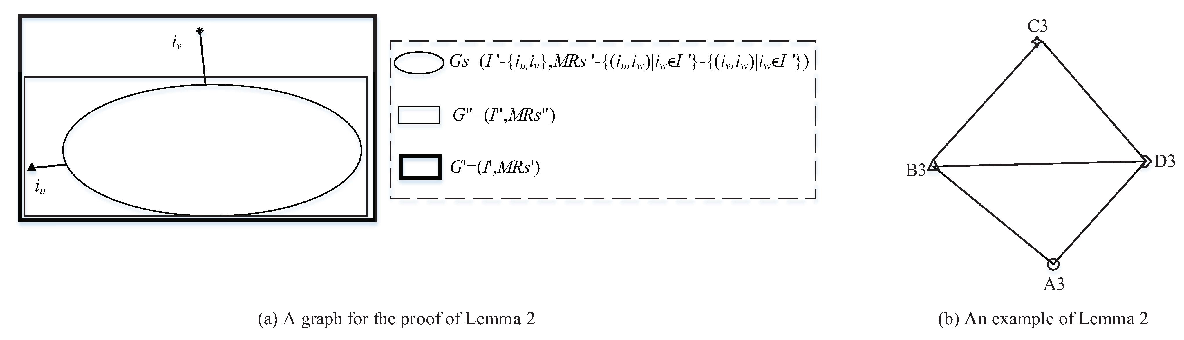
Lemma 2

(Partial antimonotonicity of minimum closeness centrality). Given a spatial mutual neighbor relationship graph $G=(I,\{(i_u,i_v)\mid i_u\in I,i_v\in MR{s}_{\alpha }\left(i_u\right)\}$, let $I^{\prime }$ be a size-k subset of I ($I^{\prime }\subseteq I\wedge k>=1$). There must exist a size-($k-1$) subset of $I^{\prime }$ (denoted $I^{″}$) to make $MCC\left(I^{″}\right)\ge MCC\left(I^{\prime }\right)$. Namely,

$$(\forall I^{\prime }\subseteq I)(\exists I^{″}\subset I^{\prime })(\mid I^{\prime }\mid \ge 1\wedge \mid I^{\prime }\mid =\mid I^{″}\mid +1\to MCC\left(I^{″}\right)\ge \left(MCC\left(I^{\prime }\right)\right))$$

(13)

Proof of Lemma 2. 

If $MCC\left(I^{″}\right)=0$, it is obviously true.

As shown in Figure 3, assuming $G^{\prime }=(I^{\prime },MR{s}^{\prime })$ is a subgraph in the mutual neighbor relationship graph $G=(I,\{(i_u,i_v)\mid i_u\in I,i_v\in MN{s}_{\alpha }\left(i_u\right)\})$ where $I^{\prime }\subseteq I$ and $MR{s}^{\prime }=\{(i_u,i_v)\mid i_u\in I^{\prime }\wedge i_v\in I^{\prime }\wedge \mid sp(i_u,i_v)\mid <\infty \}$, let $i_v$ be the farthest instance from $i_u$ in $G^{\prime }=(I^{\prime },MR{s}^{\prime })$, namely, $(\forall i_w\in I^{\prime })(\mid sp(i_u,i_v)\mid \ge \mid sp(i_u,i_w)\mid )$. Moreover, let $i_u$ be the instance making $MCC\left(I^{″}\right)=CC(I^{″},i_u)$ where $I^{″}=I^{\prime }\backslash i_v$ and $MR{s}^{″}=MR{s}^{\prime }-\{(i_v,i_w)\mid i_w\in I^{\prime }\}$. Assuming $\mid sp(i_u,i_v)\mid =\kappa$, then, $MCC\left(I^{″}\right)=CC(I^{″},i_u)=\frac{\eta -1}{\sigma }$ where $\eta =\mid I^{″}\mid$ and $\sigma ={\sum }_{i_w\in I^{″}}\mid sp(i_u,i_w)\mid$. Therefore, $MCC\left(I^{\prime }\right)\le CC(I^{\prime },i_u)=\frac{\eta -1+1}{\sigma +\kappa }=\frac{\eta }{\sigma +\kappa }$. Thus,

$$\begin{array}{cc}\hfill & MCC\left(I^{″}\right)-MCC\left(I^{\prime }\right)\hfill \\ \hfill \ge & \frac{\eta -1}{\sigma }-\frac{\eta }{\sigma +\kappa }\hfill \\ \hfill =& \frac{\eta \sigma -\sigma +\eta \kappa -\kappa -\eta \sigma }{\sigma (\sigma +\kappa )}\hfill \\ \hfill =& \frac{\eta \kappa -\sigma -\kappa }{\sigma (\sigma +\kappa )}\hfill \end{array}$$

$\because \mid sp(i_u,i_v)\mid =\kappa$

$\therefore (\forall \delta \in N^{*})(\exists i_s\in I^{\prime })(1\ge \delta \ge \kappa ,\mid sp(i_u,i_s)\mid =\delta )$ and $\kappa \le \eta -1$.

$\therefore \eta \ge \kappa +1\wedge \sigma \le 1+2+\cdots +(\kappa -1)+\kappa (\eta -1-(\kappa -1\left)\right)$. Thus,

$$\begin{array}{cc}\hfill & \eta \kappa -\sigma -\kappa \hfill \\ \hfill \ge & \eta \kappa -(1+2+\cdots +(\kappa -1)+\kappa (\eta -1-(\kappa -1)\left)\right)-\kappa \hfill \\ \hfill =& \frac{{\kappa }^2+\kappa -2}{2}\hfill \\ \hfill \because & \kappa \ge 1\hfill \\ \hfill \therefore & {\kappa }^2+\kappa -2\ge 0\hfill \\ \hfill \therefore & \frac{{\kappa }^2+\kappa -2}{2}\ge 0\hfill \\ \hfill \therefore & \eta \kappa -\sigma -\kappa \ge 0\hfill \\ \hfill \because & \sigma (\sigma +\kappa )\ge 0\hfill \\ \hfill \therefore & \frac{\eta \kappa -\sigma -\kappa }{\sigma (\sigma +\kappa )}\ge 0\hfill \\ \hfill \therefore & MCC\left(I^{″}\right)-MCC\left(I^{\prime }\right)\ge 0\hfill \\ \hfill \therefore & (\forall I^{\prime }\subseteq I)(\exists I^{″}\subset I^{\prime })(\mid I^{\prime }\mid \ge 1\wedge \mid I^{\prime }\mid =\mid I^{″}\mid +1\to MCC\left(I^{″}\right)\ge MCC\left(I^{\prime }\right))\hfill \end{array}$$

   □

Lemma 2 declares that if there is no subset whose minimum closeness centrality is less than or equal to a given float $\beta$, any of its superset besides itself cannot be less than or equal to $\beta$.

Example 7.

In Figure 2b, $MCC\left(\right\{A1,E1\left\}\right)=1/2<2/3$, $MCC\left(\right\{A1,C2\left\}\right)=1/4<2/3$, and $MCC\left(\right\{C2,E1\left\}\right)=1/2<2/3$; thus, $MCC\left(\right\{A1,C2,E1\left\}\right)<2/3$.

Definition 12

(Type-$\beta$ co-location instance). Given a pattern p ($p\subseteq F$) and $G=(I,\{(i_u,i_v)\mid i_u\in I,i_v\in MR{s}_{\alpha }\left(i_u\right)\})$, let $MCC\left(I^{\prime }\right)$ be the minimum closeness centrality of $I^{\prime }$ where $I^{\prime }\subseteq I$. If the corresponding feature set of $I^{\prime }$ is p and $MCC\left(I^{\prime }\right)\ge \beta$, where β is the given threshold by users, $I^{\prime }$ is called a type-β co-location instance of p. The set composed of all type-β co-location instances of p is called the type-β co-location table instance of p. Namely,

$$CI{s}_{\beta }\left(p\right)=\{I^{\prime }\mid I^{\prime }\subseteq I,\mid I^{\prime }\mid =\mid p\mid ,CFs\left(I^{\prime }\right)=p,MCC\left(I^{\prime }\right)\ge \beta \}$$

(14)

Example 8.

In Figure 2b, $CI{s}_{\beta }\left(\{A,B,C,D,E\}\right)=\{\{A1,B1,C1,D1,E1\},\{A2,B2,C2,D2,E1\},\{A3,B3,C3,D3,E2\}\}$ while $\beta \le 4/7$.

In comparison with Definition 2, Definition 12 is more flexible for that the minimum closeness centrality of a co-location instance $I^{\prime }$ is 1 (i.e., $\frac{\mid I^{\prime }\mid -1}{(\mid I^{\prime }\mid -1)\ast 1}$).

The minimum closeness centrality of a type-$\beta$ co-location instance $I^{\prime }$ measures the maximal distance between instance pairs. The correlation of $I^{\prime }$ can be evaluated. In other words, if $I^{\prime }$ is a type-$\beta$ co-location instance, each pair of instances in $I^{\prime }$ can be reachable from each other in an upper-bounder step.

Theorem 1

(Necessary condition of type-$\beta$ co-location instance). Given an instance set $I^{\prime }$ in $G=(I,\{(i_u,i_v)\mid i_u\in I,i_v\in MR{s}_{\alpha }\left(i_u\right)\})$, if $I^{\prime }$ is a type-β co-location instance, any pair of instance in $I^{\prime }$ can be reachable to each other in $\lceil \frac{2}{\beta }\rceil -1$ steps. Namely,

$$\begin{array}{cc}\hfill & MCC\left(I^{\prime }\right)\ge \beta \Rightarrow (\forall i_u\in I^{\prime })(\forall i_v\in I^{\prime })(0\le \mid sp(i_u,i_v)\mid \le \lceil \frac{2}{\beta }\rceil -1)\hfill \end{array}$$

(15)

Proof of Theorem 1. 

Given an instance set $I^{\prime }$ in $G=(I,\{(i_u,i_v)\mid i_u\in I,i_v\in MR{s}_{\alpha }\left(i_u\right)\})$, if $I^{\prime }$ is a type-$\beta$ co-location instance, $1\ge MCC\left(I^{\prime }\right)\ge \beta$. Let $\eta =\mid I^{\prime }\mid$. Let $i_0,i_1,\cdots ,i_{\kappa }$ be the longest shortest path between any pair of instances in $I^{\prime }$. Thus, $i_0\in I^{\prime }\wedge i_{\kappa }\in I^{\prime }$. Furthermore, $CC(I^{\prime },i_0)\ge \beta \wedge CC(I^{\prime },i_{\kappa })\ge \beta$. Moreover, for any instance $i_u$ in $I^{\prime }$ ($i_u\in I^{\prime }$), there must be $\mid sp(i_0,i_u)\mid +\mid sp(i_u,i_{\kappa })\mid \ge \mid sp(i_0,i_k)\mid =\mid \{i_0,i_1,\cdots ,i_k\}\mid =\kappa$. Therefore, to adopt the maximal $\kappa$ in $I^{\prime }$, let any instance $i_u$ in $I^{\prime }$ ($i_u\in I^{\prime }$), making $\mid sp(i_0,i_u)\mid +\mid sp(i_u,i_{\kappa })\mid =\kappa$ while letting $MCC\left(I^{\prime }\right)=\beta$. That is to say, $MCC\left(I^{\prime }\right)=\frac{\eta -1}{\lceil \frac{\eta \kappa }{2}\rceil }=\beta$ makes $\kappa$ be maximal. Thus, $\kappa \le \lfloor \frac{2}{\beta }-\frac{2}{\eta \beta }\rfloor$. Because $\kappa \in N^{*}$ and $0\le \beta \le 1$, $\eta \beta$ can be much larger than $\beta$. Thus, $\frac{2}{\beta }>>\frac{2}{\eta \beta }$. Therefore, $(\forall i_u\in I^{\prime })(\forall i_v\in I^{\prime })(1\le \mid sp(i_u,i_v)\mid \le \lceil \frac{2}{\beta }\rceil -1)$.    □

Theorem 1 declares that there exists a strong correlation among type-$\beta$ co-location instances. For example, if $\beta =1$, any pair of instances can be reachable to each other in 1 (i.e., $\lceil \frac{2}{1}\rceil -1$) step. It is a clique at least. Similarly, if $\beta \ge 4/5$, any pair of instances can be reachable to each other in 2 (i.e., $\lceil \frac{2}{4/5}\rceil -1$) steps. It is a star at least. If $\beta \ge 1/2$, any pair of instances can be reachable to each other in 3 (i.e., $\lceil \frac{2}{1/2}\rceil -1$) steps. If $\beta \ge 2/5$, any pair of instances can be reachable to each other in 4 (i.e., $\lceil \frac{2}{2/5}\rceil -1$) steps. If $\beta \ge 1/3$, any pair of instances can be reachable to each other in 5 (i.e., $\lceil \frac{2}{1/3}\rceil -1$) steps. The rest can be carried out in the same manner.

Unfortunately, if every instance pair in an instance subset $I^{\prime }$ can be reachable to each other in $\lceil \frac{2}{\beta }\rceil -1$ steps, $MCC\left(I^{\prime }\right)\ge \beta$ is not necessarily true. That is to say, it is a necessary condition but not necessarily sufficient.

Example 9. 

$MCC\left(\{A1,B1,C1,D1,E1\}\right)=4/7\Rightarrow (\forall i_u\in \{A1,B1,C1,D1,E1\})(\forall i_v\in \{A1,B1,C1,D1,E1\})(\mid sp(i_u,i_v)\mid \le \lceil \frac{2}{7/4}\rceil -1=3)$. On the contrary, $\lceil \frac{2}{\beta }\rceil -1=2$ but $MCC\left(\{A1,E1\}\right)=\frac{2-1}{2}=\frac{1}{2}<\beta$ when β = 2/3 in Figure 2b.

According to Lemma 2 and Theorem 1, candidate type-$\beta$ co-location instance can be pruned well. That is to say, if there is an instance pair in a candidate type-$\beta$ co-location, instance $I^{\prime }$ cannot be reachable to each other in $\lceil \frac{2}{\beta }\rceil -1$ steps, so it cannot be true. Furthermore, if there is no size-($\mid I^{\prime }\mid -1$) subset of $I^{\prime }$ being a type-$\beta$ co-location instance, it still must not be a type-$\beta$ co-location instance.

Definition 13

(Type-$\beta$ participation ratio). Let $CI{s}_{\beta }\left(p\right)$ be the type-β co-location table instance of a pattern p. The type-β participation ratio of a feature $f_i$ in p is the ratio of closeness centrality summary of $f_i$’s instances appearing in $CI{s}_{\beta }\left(p\right)$ to instances of $f_i$. Namely,

$$\begin{array}{cc}\hfill P{R}_{\beta }(p,f_i)=& \frac{{\sum }_{i_u\in \cup CI{s}_{\beta }\left(p\right)\wedge fea\left(i_u\right)=f_i}CC(I^{\prime },i_u)}{\mid \{i_u\mid i_u\in I\wedge i_u\notin \cup CI{s}_{\beta }\left(p\right)\wedge fea\left(i_u\right)=f_i\}+\mid CI{s}_{\beta }\left(p\right)\mid }\hfill \end{array}$$

(16)

Example 10.

$P{R}_{\beta }(\{A,B,C,D,E\},E)=\frac{4/7+4/7+4/6}{3}=40/63$ in Figure 2b while $\beta \le 4/7$. It is different from $PR\left(\right\{A,B,C,D,E\},E)=0$ in Definition 3.

The reason why not to use $P{R}_{\beta }(p,f_i)=\frac{{\sum }_{i_u\in \cup CI{s}_{\beta }\left(p\right)\wedge fea\left(i_u\right)=f_i}CC(I^{\prime },i_u)}{\mid \{i_u\mid i_u\in I\wedge fea\left(i_u\right)=f_i\}\mid }$ is that an instance may repeatedly appear in different type-$\beta$ co-location instances.

Definition 14

(Type-$\beta$ participation index). Given a pattern p ($p\subseteq F$), its type-β participation index is the minimum type-β participation ratio of features in p. Namely,

$$P{I}_{\beta }\left(p\right)=mi{n}_{f_i\in p}P{R}_{\beta }(p,f_i)$$

(17)

Example 11.

$P{I}_{\beta }\left(\{A,B,C,D,E\}\right)=min(\frac{4/5+4/5+4/5}{3},\frac{4/5+4/4+4/5}{3},\frac{4/5+4/5+4/4}{3},\frac{4/4+4/4+4/4}{3},\frac{4/7+4/6+4/6}{3})=40/63$ in Figure 2b while $\beta \le 4/7$. It is different from $PI\left(\right\{A,B,C,D,E\left\}\right)=0$ in Definition 3.

Definition 15

(Type-$\beta$ co-location pattern). Given a pattern p ($p\subseteq F$) and a prevalence threshold ζ, if and only if $P{I}_{\beta }\left(p\right)\ge \zeta$, we call p a type-β co-location pattern. The set composed of all type-β co-location patterns is denoted $CP{s}_{\beta }$. Namely,

$$P{I}_{\beta }\left(p\right)\ge \zeta \iff p\in CP{s}_{\beta }$$

(18)

Example 12.

{A, B, C, D, E} is a type-β co-location pattern when $\beta \le 4/7\wedge \zeta \le 40/63$, but it is not a co-location pattern in Definition 4 when $min\_pi>0$ in Figure 2b.

Perhaps any nonempty subset of F can be theoretically a candidate type-$\beta$ co-location pattern. If all $2^{\mid F\mid }-\mid F\mid -1$ candidate patterns are checked in turn with their type-$\beta$ co-location instance generation, it is time-consuming. In comparison with Lemma 1, the a priori property is not satisfied to type-$\beta$ co-location patterns because of Lemma 2. Thus, we firstly introduce the approximate type-$\beta$ co-location pattern to avoid combination explosion, and then propose a new property in Theorem 1.

Definition 16

(Approximate type-$\beta$ co-location pattern). Given a pattern p ($p\subseteq F$) and a prevalence threshold ζ, if its type-β participation index is greater than or equal to ζ when its type-β co-location instances are relaxed as instance pairs and can be reachable to each other in $\lceil \frac{2}{\beta }\rceil -1$ steps, p is called an approximate type-β co-location pattern. The set composed of approximate type-β co-location patterns is denoted by $AP{s}_{\beta }$. Namely,

$$mi{n}_{f_i\in p}\left\{\frac{\mid \{i_u\mid i_u\in \cup UI{s}_{\beta }\left(p\right)\wedge fea\left(i_u\right)=f_i\}\mid }{\mid \{i_u\mid i_u\in I\wedge fea\left(i_u\right)=f_i\}\mid }\right\}\ge \zeta \iff p\in AP{s}_{\beta }$$

(19)

where $UI{s}_{\beta }\left(p\right)=\{I^{\prime }\mid (\forall i_v\in I^{\prime })(\forall i_w\in I^{\prime })(I^{\prime }\subseteq I\wedge \{fea\left(i_s\right)\mid i_s\in I^{\prime }\}=p\wedge \mid I^{\prime }\mid =\mid p\mid \wedge \mid sp(i_v,i_w)\mid \le \lceil \frac{2}{\beta }\rceil -1)\}$.

Example 13.

$\{A,B,C,D,E,F\}\in AP{s}_{\beta }$ when $\beta \le 4/7$ and $\zeta \le 2/3$, but $P{I}_{\beta }\left(\{A,B,C,D,E,F\}\right)$$=5/21$.

Theorem 2

(Downward closure of approximate type-$\beta$ co-location pattern). Given a subset p of the feature set F ($p\subseteq F$), if p is an approximate type-β co-location pattern, any subset of p must also be an approximate type-β co-location pattern. Namely,

$$\begin{array}{c}\hfill (\forall p\subseteq F)(\forall p^{\prime }\subseteq p)(p\in AP{s}_{\beta }\to p^{\prime }\in AP{s}_{\beta })\end{array}$$

(20)

Proof of Theorem 2. 

Given two subsets p and $p^{\prime }$ of the feature set F ($p^{\prime }\subset p\subseteq F$), let $f_i$ be a feature in $p^{\prime }$ ($f_i\in p^{\prime }\wedge f_i\in p$). Assuming $I^{\prime }$ is any instance subset satisfying to $(\forall i_v\in I^{\prime })(\forall i_w\in I^{\prime })(I^{\prime }\subseteq I\wedge \{fea\left(i_s\right)\mid i_s\in I^{\prime }\}=p\wedge \mid I^{\prime }\mid =\mid p\mid \wedge \mid sp(i_v,i_w)\mid \le \lceil \frac{2}{\beta }\rceil -1)$, it is understandable that any subset of $I^{″}$, whose corresponding feature set is $p^{\prime }$, can satisfy to $(\forall i_v\in I^{″})(\forall i_w\in I^{″})(I^{″}\subseteq I^{\prime }\wedge \{fea\left(i_s\right)\mid i_s\in I^{″}\}=p^{\prime }\wedge \mid I^{″}\mid =\mid p^{\prime }\mid \wedge \mid sp(i_v,i_w)\mid \le \lceil \frac{2}{\beta }\rceil -1)$. That is to say, if an instance $i_u$ whose feature is $f_i$ appears in $I^{\prime }$, it also must appear in $I^{″}$. Thus, $\frac{\mid \{i_u\mid i_u\in \cup UI{s}_{\beta }\left(p\right)\wedge fea\left(i_u\right)=f_i\}\mid }{\mid \{i_u\mid i_u\in I\wedge fea\left(i_u\right)=f_i\}\mid }\le \frac{\mid \{i_u\mid i_u\in \cup UI{s}_{\beta }\left(p^{\prime }\right)\wedge fea\left(i_u\right)=f_i\}\mid }{\mid \{i_u\mid i_u\in I\wedge fea\left(i_u\right)=f_i\}\mid }$, and then $\frac{\mid \{i_u\mid i_u\in \cup UI{s}_{\beta }\left(p\right)\wedge fea\left(i_u\right)=f_i\}\mid }{\mid \{i_u\mid i_u\in I\wedge fea\left(i_u\right)=f_i\}\mid }\ge \zeta \Rightarrow \frac{\mid \{i_u\mid i_u\in \cup UI{s}_{\beta }\left(p^{\prime }\right)\wedge fea\left(i_u\right)=f_i\}\mid }{\mid \{i_u\mid i_u\in I\wedge fea\left(i_u\right)=f_i\}\mid }\ge \zeta$. A more detailed proof can be modeled on the proof of the antimonotonicity of participation ratios and participation indexes in [31].

Furthermore,

$$\begin{array}{cc}\hfill & mi{n}_{f_i\in p^{\prime }}\left\{\frac{\mid \{i_u\mid i_u\in \cup UI{s}_{\beta }\left(p^{\prime }\right)\wedge fea\left(i_u\right)=f_i\}\mid }{\mid \{i_u\mid i_u\in I\wedge fea\left(i_u\right)=f_i\}\mid }\right\}\hfill \\ \hfill \ge & min\{mi{n}_{f_i\in p^{\prime }}\left\{\frac{\mid \{i_u\mid i_u\in \cup UI{s}_{\beta }\left(p^{\prime }\right)\wedge fea\left(i_u\right)=f_i\}\mid }{\mid \{i_u\mid i_u\in I\wedge fea\left(i_u\right)=f_i\}\mid }\right\},\hfill \\ & mi{n}_{f_j\in p-p^{\prime }}\left\{\frac{\mid \{i_u\mid i_u\in \cup UI{s}_{\beta }\left(p\right)\wedge fea\left(i_u\right)=f_j\}\mid }{\mid \{i_u\mid i_u\in I\wedge fea\left(i_u\right)=f_j\}\mid }\right\}\hfill \\ \hfill \ge & min\{mi{n}_{f_i\in p^{\prime }}\left\{\frac{\mid \{i_u\mid i_u\in \cup UI{s}_{\beta }\left(p\right)\wedge fea\left(i_u\right)=f_i\}\mid }{\mid \{i_u\mid i_u\in I\wedge fea\left(i_u\right)=f_i\}\mid }\right\},\hfill \\ & mi{n}_{f_j\in p-p^{\prime }}\left\{\frac{\mid \{i_u\mid i_u\in \cup UI{s}_{\beta }\left(p\right)\wedge fea\left(i_u\right)=f_j\}\mid }{\mid \{i_u\mid i_u\in I\wedge fea\left(i_u\right)=f_j\}\mid }\right\}\hfill \\ \hfill =& min\{mi{n}_{f_i\in p}\left\{\frac{\mid \{i_u\mid i_u\in \cup UI{s}_{\beta }\left(p\right)\wedge fea\left(i_u\right)=f_i\}\mid }{\mid \{i_u\mid i_u\in I\wedge fea\left(i_u\right)=f_i\}\mid }\right\}\hfill \end{array}$$

Namely,

$$\begin{array}{cc}\hfill & mi{n}_{f_i\in p}\left\{\frac{\mid \{i_u\mid i_u\in \cup UI{s}_{\beta }\left(p\right)\wedge fea\left(i_u\right)=f_i\}\mid }{\mid \{i_u\mid i_u\in I\wedge fea\left(i_u\right)=f_i\}\mid }\right\}\ge \zeta \wedge p^{\prime }\subseteq p\hfill \\ \hfill \Rightarrow & mi{n}_{f_i\in p^{\prime }}\left\{\frac{\mid \{i_u\mid i_u\in \cup UI{s}_{\beta }\left(p^{\prime }\right)\wedge fea\left(i_u\right)=f_i\}\mid }{\mid \{i_u\mid i_u\in I\wedge fea\left(i_u\right)=f_i\}\mid }\right\}\ge \zeta \hfill \end{array}$$

Thus,

$$(\forall p\subseteq F)(\forall p^{\prime }\subseteq p)(p\in AP{s}_{\beta }\to p^{\prime }\in AP{s}_{\beta })$$

   □

Example 14.

$\{A,B,C,D,E,F\}\in AP{s}_{\beta }$ when $\beta \le 4/7$ and $\zeta \le 2/3$, so are any subset of $\{A,B,C,D,E,F\}$.

By comparing Definitions 15 and 16, Theorem 2 declares that a pattern cannot be a type-$\beta$ co-location pattern until there is no subset not being an approximate type-$\beta$ co-location pattern, since the closeness centrality of an instance is greater than or equal to 0 and less than or equal to 1. At this point, this type-$\beta$ co-location pattern mining problem can be transformed into the classical co-location pattern mining problem. Therefore, the majority of traditional co-location pattern mining algorithms such as Join-based, Join-less [32], CPI-tree, and so on can be improved to mine type-$\beta$ co-location patterns.

For a type-$\beta$ co-location instance, each instance has closeness centrality. Accordingly, for a type-$\beta$ co-location pattern, each feature has closeness centrality.

Definition 17

(Closeness centrality of $f_i$ ($f_i\in p,p\subseteq F$)). Given a type-β co-location pattern p, let $f_i$ be any feature in p. The closeness centrality of $f_i$ in p is the average closeness centrality of instances carrying $f_i$ in its type-β co-location instances. Namely

$$CCF(p,f_i)=\frac{{\sum }_{i_u\in I^{\prime },I^{\prime }\in CI{s}_{\beta }\left(p\right),fea\left(i_u\right)=f_i}CC(I^{\prime },i_u))}{\mid CI{s}_{\beta }\left(p\right)\mid }$$

(21)

Example 15.

$CCF\left(\right\{A,B,C,D,E\},A)=4/5=0.8$, $CCF\left(\right\{A,B,C,D,E\},B)=13/15\approx 0.87$, $CCF\left(\right\{A,B,C,D,E\},C)=13/15\approx 0.87$, $CCF\left(\right\{A,B,C,D,E\},D)=1$, and $CCF\left(\right\{A,B,C,D,E\},E)=40/63\approx 0.63$ when $\beta \le 4/7$ and $\zeta \le 40/63$ in Figure 2b.

The reason to not let the denominator be $\mid \{i_u\mid (\exists s\in CIs\left(p\right))(i_u\in s,fea\left(i_u\right)=f_i)\}\mid$ instead of $\mid CIs\left(p\right)\mid$ to be more intuitive is that an instance $i_u$ may appear in different type-$\beta$ co-location instances of p.

Since the closeness centrality of every instance in a type-$\beta$ co-location pattern instance is greater than or equal to $\beta$ according to Definition 12, the closeness centrality of every feature in a type-$\beta$ co-location pattern must also be greater than or equal to $\beta$ according to Definition 17. Furthermore, the closeness centrality of each feature in a type-$\beta$ co-location pattern may be different. That is to say, in a type-$\beta$ co-location pattern, the correlation between a feature and the other feature may be different. Some features may be in the center of topology of the pattern while the others on the edge. The feature with high closeness centrality are more correlated to other features. Obviously, the closer $CCF(p,f_i)$ reaches to 1, the higher the correlation with the other features $f_i$ has in p when the distribution of the whole data set is taken into account.

The closeness centrality of instances in an instance subset $I^{\prime }$ can be different even if $I^{\prime }$ is a clique. Therefore, Definition 17 can be improved. By the way, this does not apply to Definition 12. In this paper, we focus on Definition 17 but not Definition 18.

Definition 18

(Extended closeness centrality of $f_i$ ($f_i\in p,p\subseteq F$)). Given a type-β co-location pattern p, let $f_i$ be any feature in p. The extended closeness centrality of $f_i$ in p is the average closeness centrality on distances of instances carrying $f_i$ in its type-β co-location instances. Namely,

$$ECCF(p,f_i)=\frac{{\sum }_{i_u\in I^{\prime },I^{\prime }\in CI{s}_{\beta }\left(p\right),fea\left(i_u\right)=f_i}ECC(I^{\prime },i_u)}{\mid CI{s}_{\beta }\left(p\right)\mid }$$

(22)

where $ECC(I^{\prime },i_u)=\frac{min\_weights\left(I^{\prime }\right)}{{\sum }_{i_v\in I^{\prime }}dis(i_u,i_v)}$ and $min\_weights\left(I^{\prime }\right)$ is the summary of edge weights in the minimum spanning tree [33] of $G^{\prime }=(I^{\prime },\{(i_u,i_v)\mid i_u\in I^{\prime }\wedge i_v\in I^{\prime }\},\{dis(i_u,i_v)\mid i_u\in I^{\prime }\wedge i_v$$\in I^{\prime }\left\}\right)$.

Example 16.

$ECCF(\{A,B,C\},A)=\frac{(3+3.2)/(3+3.2)+(5.6+5.1)/(5.6+5.1)+(11.2+11.6)/(11.6+16.2)}{3}\approx 0.94$, $ECCF(\{A,B,C\},B)=\frac{(3+3.2)/(3+3.6)+(5.6+5.1)/(5.6+5.8)+(11.2+11.6)/(11.6+11.2)}{3}\approx 0.96$, $ECCF(\{A,B,C\},C)=\frac{(3+3.2)/(3.2+3.6)+(5.6+5.1)/(5.1+5.8)+(11.2+11.6)/(11.2+16.2)}{3}\approx 0.91$ when $\beta \le 1$ and $\zeta \le 1$, but $CCF\left(\right\{A,B,C\},A)=1$, $CCF\left(\right\{A,B,C\},B)=1$, $CCF\left(\right\{A,B,C\},C)=1$ in Figure 2b.

Obviously, $0\le ECC(I^{\prime },i_u)\le 1$ for any instance $i_u$ in an instance subset $I^{\prime }$. Furthermore, Definition 18 normalizes the closeness centrality of all features in their corresponding patterns. That is to say, the closer $ECCF(p,f_i)$ reaches to 1, the highercorrelation between $f_i$ and the other features in p when the distributions of type-$\beta$ co-location instances are just taken into account, rather than of all instances.

Since the closeness centrality of each feature in prevalent patterns is expected to be evaluated, an algorithm based on Join-less in a size-wised manner rather than in a maximal pattern [34] finding way is proposed in this paper.

4.2. Type-$\beta$ Co-Location Pattern Mining

Given that Join-less does not take closeness centrality into account, it should be improved in aspects as follows. (a) Path lengths between instance pairs should be calculated by the shortest path algorithms such as the algorithm of Dijkstra in $G=(V,E)$ (the output of Algorithm 1), and then, if the path length between an instance pair is not greater than $\lceil \frac{2}{\beta }\rceil -1$, update an edge between the pair of instances according to Theorem 1. (b) All approximate type-$\beta$ co-location patterns and their instances are adopted on the updated $G=(V,E)$ by Join-less according to Theorem 2. (c) Check the prevalence of each approximate type-$\beta$ co-location pattern on their instances with Theorem 1 and Definition 15. (d) For each type-$\beta$ co-location pattern, the closeness centrality of each feature can be computed in Definition 17 or Definition 18.

Algorithm 2 is used to find type-$\beta$ co-location patterns with their feature closeness centrality values. Next, we read the algorithm and analyze the time complexity. Step 1 generates a mutual neighbor relationship graph by Algorithm 1. It costs $O(\mid I{\mid }^2)$. Step 2 returns the shortest path lengths between each instance pair by the algorithm of Dijkstra. It costs $O(\mid E{\mid }^2)$. Steps 3 to 9 update the mutual neighbor relationship graph according to Theorem 1. They cost $O(\mid I{\mid }^2)$. Since every instance pair between which the shortest path length is not greater than $\lceil \frac{2}{\beta }\rceil -1$ can be detected, no approximate type-$\beta$ co-location pattern can be neglected in Step 10. Step 10 determines the time complexity of the whole algorithm. It is acknowledged that Join-less is efficient, thus so is this algorithm. Steps from 11 to 19 tend to adopt type-$\beta$ co-location patterns and compute its feature closeness centrality from approximate type-$\beta$ co-location patterns. In Step 15, feature closeness centrality is computed according to Lemma 2. This step costs $O(\mid p{\mid }^2)$. These 9 steps cost $O(\mid AP{s}_{\beta }\mid \times \frac{\mid I\mid }{\mid F\mid }\times \mid p{\mid }^2)$ in average. The whole algorithm is based on proved lemmas and theorems. Thus, it is correct and complete.

Algorithm 2 Mining type-$\beta$ co-location patterns ($\beta$-CPM)

Require:D (the given data set), F (the feature set), I (the instance set with location information), $\alpha$ the elastic coefficient to generate mutual neighbor relationships, $\beta$ the threshold for closeness centrality, $\zeta$ (the given prevalence threshold).

Ensure:$CP{s}_{\beta }$ (type-$\beta$ co-location patterns with closeness centrality of each feature).

1: G = Algorithm 1 (D, $\alpha$) //Generate spatial mutual neighbor relationship graph.

2: $\{\mid sp(i_u,i_v)\mid \mid i_u\in I\wedge i_v\in I\}=Dijkstra\left(G\right)$ //Get shortest path lengths between instance pairs.

3: for $i_u\in I$ do

4:    for $i_v\in I$ do

5:      if $\mid sp(i_u,i_v)\mid \le \lceil \frac{2}{\beta }\rceil -1$ then

6:         $E=E\cup \left\{(i_u,i_v)\right\}$ //Theorem 1.

7:      end if

8:    end for

9: end for

10: $AP{s}_{\beta },AP{s}_{\beta }\_ins=Join-less(data=G,min\_pi=\beta )$ //Theorem 2.

11: for $p\in AP{s}_{\beta }$ do

12:    if $check\_CP{s}_{\beta }(p,AP{s}_{\beta }\_ins)$ then

13:      $p\_dict=\left\{\right\}$

14:      for $f_i\in p$ do

15:         $p\_dict.update\left(\{f_i:CCF(p,f_i)\}\right)$ //Definition 17/ 18 and Lemma 2.

16:      end for

17:      $CP{s}_{\beta }=CP{s}_{\beta }\cup \{p\_dict\}$ //Definition 15.

18:    end if

19: end for

20: return $CP{s}_{\beta }$

5. Experiment Analysis

In this section, both synthetic and real data sets are used to design our experiments. The reason for using the synthetic data set is that it is difficult to evaluate what can be the ideal result on the real data set.

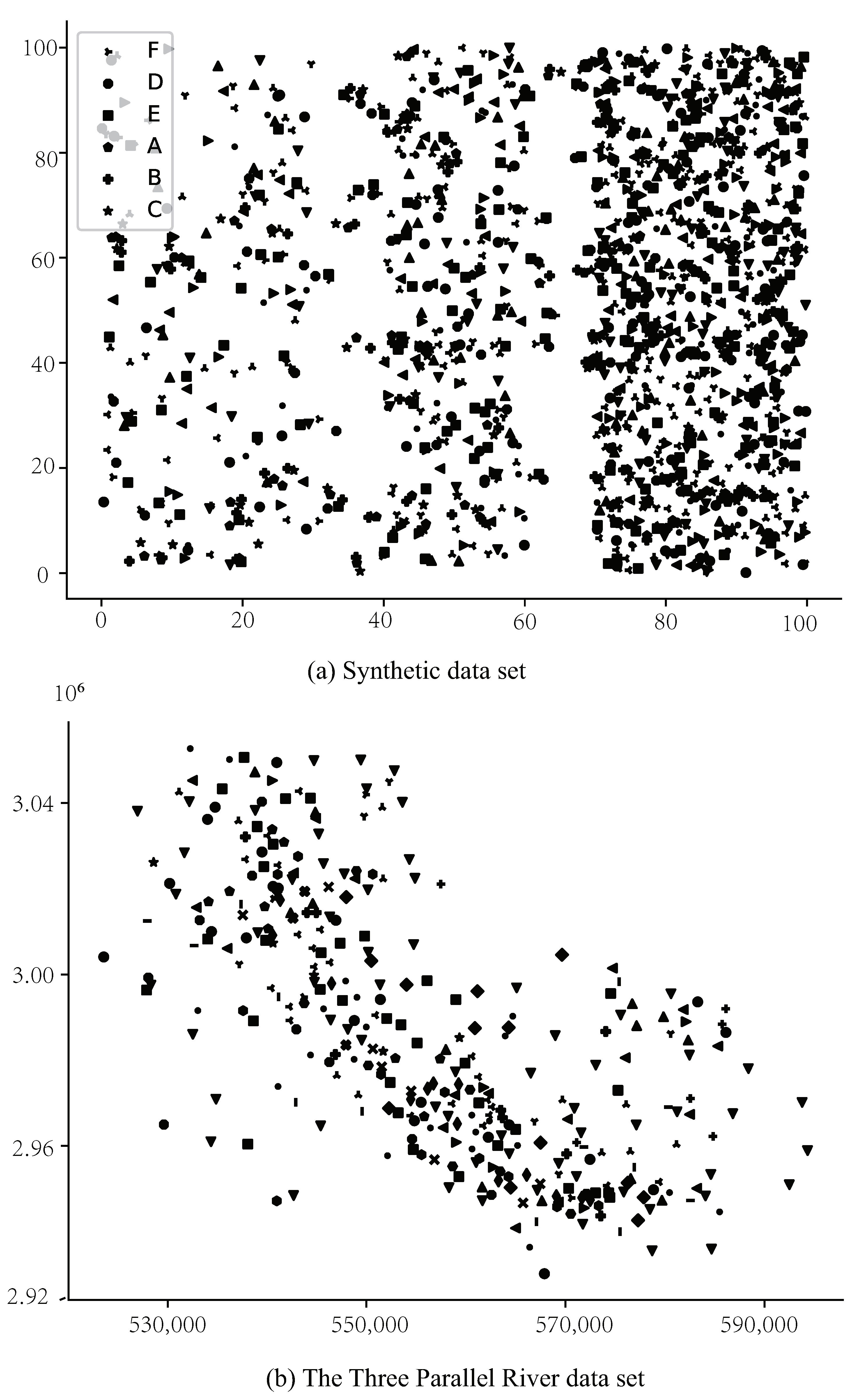
Synthetic data setFigure 4a shows the synthetic data set, called Synthetic data set, produced by us. The space is divided into three regions of similar areas. Coordinates of instances are randomly assigned in each region following the distribution densities of 3:8:13. Moreover, instances carrying features in {A, B, C} are deliberately arranged to gather, and so are they in {D, E, F}. The densities of instances of both {A, B, C} and {D, E, F} are higher than their corresponding regional densities (the average distance of pair instance neighbors is not greater than 6 m, 4 m, and 2 m in the corresponding three regions, respectively). In other words, {A, B, C} and {D, E, F} can be interesting patterns but others not.

The Three Parallel River data setFigure 4b shows the distributions of the rare plants in the Three Parallel Rivers (short for the Three Parallel River data set). It is generally sparse, but the density distribution varies greatly.

Table 1. The distributions of features and instances in the experimental data sets.

Data Sets	Feature Count	Instance Count	Distribution Densities
Synthetic data set	16	1515	Density ratios of 3:8:13
The Three Parallel Rivers data set	31	337	More different densities

shows the feature and instance distributions. Some key performance indicators are tested as follows.

5.1. Precision, Accuracy, and Recall

The precision, accuracy, and recall are, respectively, tested on the Synthetic data set, while they cannot be objectively evaluated in true data sets. In the Synthetic data set, {A, B, C} and {D, E, F} are thought to be highly correlated along with their non-size-1 subsets. In other words, {A, B}, {A, C}, {B, C}, {A, B, C}, {D, E}, {D, F},{E, F}, and {D, E, F} can be considered as positive patterns, while other $2^{\mid F\mid }-\mid F\mid -1-8$ non-size-1 ones can be carried out as negative patterns. Based on the mining results, we denote true positive patterns as $TP$, false positive patterns as $FP$, true negative patterns as $TN$, and false negative patterns as $FN$, borrowing definitions from [35]. Along this line, the precision of our algorithm (Algorithm 2) can be proposed as $\frac{\mid TP\mid }{\mid TP\mid +\mid FP\mid }$ and the accuracy can be performed as $\frac{\mid TP\mid +\mid TN\mid }{\mid TP\mid +\mid TN\mid +\mid FP\mid +\mid FN\mid }$, while the recall can be carried out as $\frac{\mid TP\mid }{\mid TP\mid +\mid FN\mid }$.

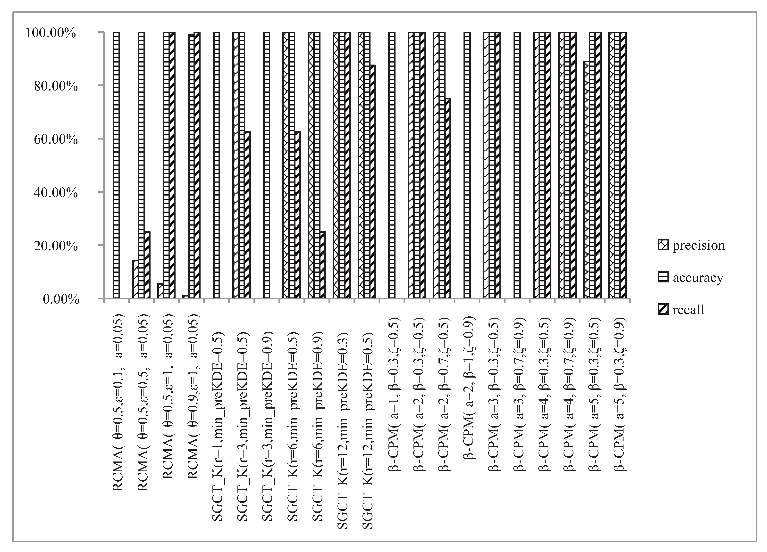
Figure 5 shows the precision, accuracy, and recall of $\beta$-CPM in different representative parameters in the Synthetic data set in comparison with RMCA [15] and SGCT_K [13]. The precision and recall are difficult to balance, while the accuracy is preferred in RCMA. Meanwhile, the balance points of the precision, accuracy, and recall of SGCT_K are difficult to find by users as they have very narrow ranges. Moreover, since participation indexes are based on Kernel functions in SGCT_K, the optimal participation index threshold is not easy to estimate by users. All positive patterns should be theoretically discovered once $r\ge 6$. However, the SGCT_K cannot perform it because of Kernel functions. Fortunately, our $\beta$-CPM is robust to work well. That any of $\alpha$, $\beta$, and $\zeta$ is optimal can lead to an optimal result.

Figure 5 also reveals that negative patterns are insensitive to $\alpha$ and $\beta$. That is to say, negative patterns are not easy to be discovered by $\beta$-CPM. Furthermore, a lower $\beta$ can make up for the fact that $\alpha$ is too small. On the contrary, a bigger $\alpha$ can also make up for the fact that $\beta$ is too big.

5.2. Efficiency

Since spatial data sets are large or even massive, users are also interested in the total time costs of algorithms.

Table 2. The total time costs (microseconds) in algorithms with ideal parameters.

Algorithms	Synthetic Data Set	The Three Parallel Rivers Data Sets
RCMA	3,492,173,294 ($\theta$ = 0.5, $ϵ$ = 0.5, $\alpha$ = 0.05)	$1.133\times {10}^{11}$ ($\theta$ = 0.5, $ϵ$ = 0.2, $\alpha$ = 0.05)
SGCT_K	6,408,119 (r = 12, $min\_preKDE$ = 0.3)	1,129,484 (r = 8000, $min\_preKDE$ = 0.3)
$\beta$-CPM	208,859 ($\alpha$ = 2, $\beta$ = 0.3, $\zeta$ = 0.5)	136,428 ($\alpha$ = 3, $\beta$ = 0.5, $\zeta$ = 0.5)

shows the total time costs of $\beta$-CPM on the Synthetic data set and the Three Parallel Rivers data set in comparison with RCMA and SGCT_K with optimal parameters. RCMA is time-consuming because its iterations are based on the dynamic k of KNN. If data sets are distributed evenly, it must drive global co-location pattern mining. In other words, it is necessary to repeatedly find patterns to check the similarity of regions to be connected. Thus, it is workable to find regional co-location patterns instead of global ones while distribution densities are different. SGCT_K focuses on the influence of distances on proximity. That is to say, it considers that the closer the more important. It neglects the influence of local distribution densities on proximity. In a word, it is irrelevant to the direction considered of our $\beta$-CPM in this article. $\beta$-CPM is more efficient than the other two with similar pattern results because it detects valuable neighbors.

5.3. Density Response

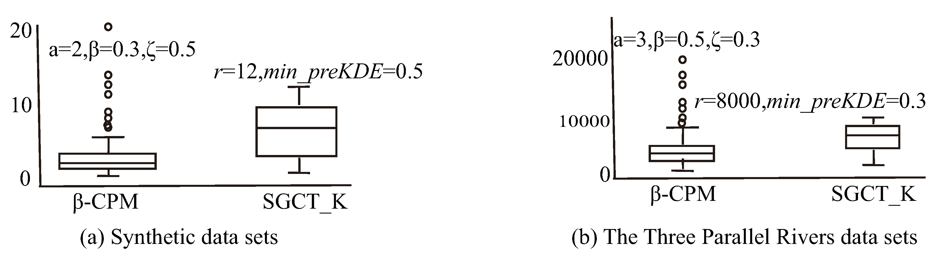
Figure 6 shows the distance distributions of neighbor pairs by $\beta$-CPM in the Synthetic data set and the Three Parallel Rivers data set in comparison with the ones by SGCT_K. Since RCMA focuses on regional co-location patterns, we no longer compare $\beta$-CPM with it.

There are almost no singularities in the boxplots of SGCT_K in both Figure 6a,b. The reason is that neighbors are defined on a global static distance threshold, while distances between instance pairs tend to be normally distributed. However, users care so much about prevalent patterns that they may not care about particular neighbor relationships of instances. In other words, there are too many neighbor pairs. More importantly, SGCT_K neglects the influences of distribution densities under Tobler’s First Law of Geography. $\beta$-CPM discovers fewer neighbor pairs but it still finds interesting patterns. The singularities reveal that there are some sparse areas in the space. It effectively responds to the influence of regional distribution density on Tobler’s First Law of Geography.

5.4. Feature Closeness Centrality

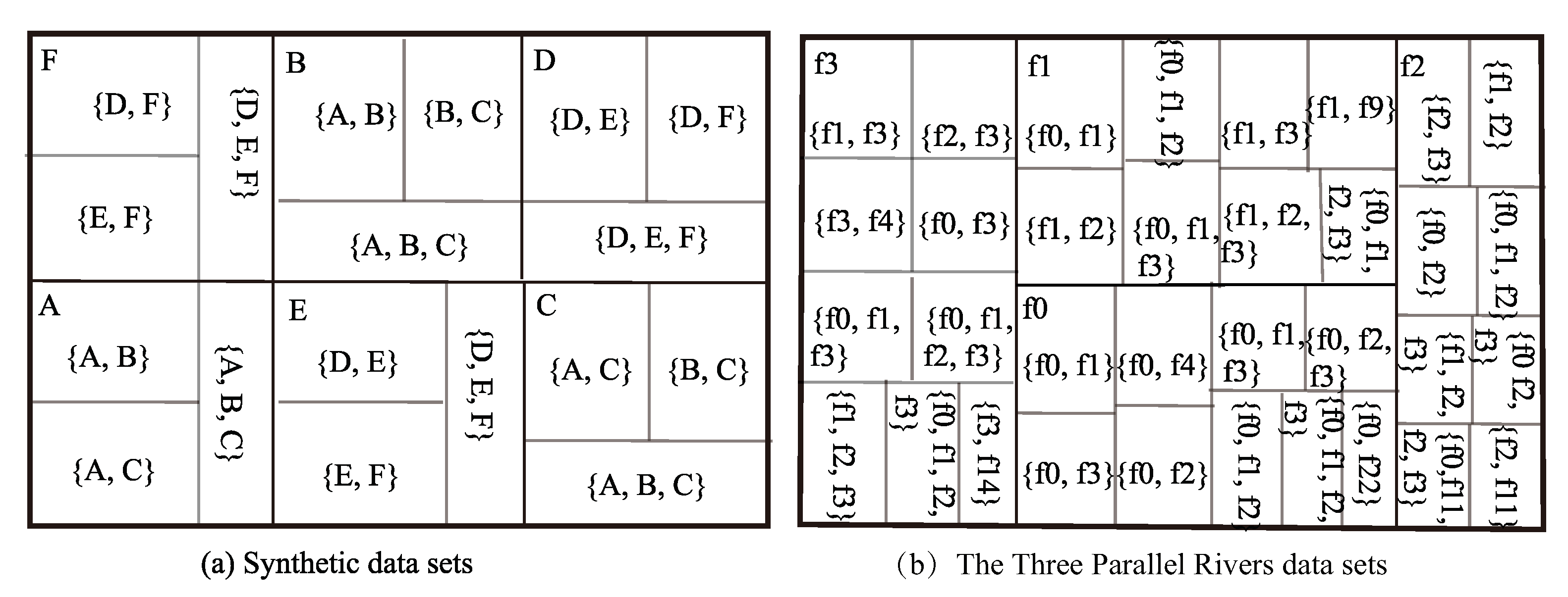
In a traditional prevalent pattern, there are only participation ratios but not closeness centrality values for features. Figure 7 shows example dendrograms of feature closeness centrality in the Synthetic data set and the Three Parallel Rivers data set. It reveals that the antimonotonicity of approximate type-$\beta$ co-location patterns may sometimes lead to the antimonotonicity of type-$\beta$ co-location patterns. Furthermore, different features may have different closeness centrality. For example, A has a higher closeness centrality than B in {A, B}, as shown in Figure 7, while $\alpha$ = 2, $\beta$ = 0.3, and $\zeta$ = 0.5.

To sum up, $\beta$-CPM is workable in precision, accuracy, recall, efficiency, density response, and feature closeness centrality expression.

6. Conclusions and Discussion

In this paper, type-$\beta$ co-location patterns are discovered in an innovative way. Firstly, spatial mutual neighbor relationships are generated on the idea the distances between an instance and its neighbors are similar but not remarkably different. This method is adaptive to different distribution densities in regions and data sets. This leads to fewer neighbor pairs but effective responses to the interests of users about expected positive patterns. Secondly, instances of interesting patterns are proposed on closeness centrality instead of on cliques or stars. It extends the formats of pattern instances and counteracts the adverse effects of a too small $\alpha$. Users can flexibly set $\beta$ according to their own preferences to control the strength of the correlation of instances. Thirdly, the closeness centrality of each feature in interesting patterns is measured by the closeness centrality of objects in instances of patterns. It can reveal the correlations between each feature and the others in a type-$\beta$ co-location pattern. A feature with higher closeness centrality condenses the type-$\beta$ co-location pattern more.

The same features have different closeness centrality in different type-$\beta$ co-location patterns. Therefore, exploring the law that the closeness centrality of features changes with the size growth of patterns can further reveal the interaction mechanism among spatial features. In addition, as the pattern size grows, features that have had higher closeness centrality suddenly descend to a minimum, and an in-depth analysis of the reasons for this can help us further understand how the patterns survive and how the correlations among features provide vitality for the survival of patterns. All of the above will be our main future work.

References

- Wang, X.; Lei, L.; Wang, L.; Yang, P.; Chen, H. Spatial co-location pattern discovery Incorporating Fuzzy Theory. IEEE Trans. Fuzzy Syst. 2021, 30, 2055–2072. [Google Scholar] [CrossRef]
- Wang, L.Z.; Fang, Y.; Zhou, L. Preference-Based Spatial Co-Location Pattern Mining; Big Data Management Series; Springer: Singapore, 2022. [Google Scholar] [CrossRef]
- Darwin, C. The Origin of Species; Manchester University Press: Manchester, UK; New York, NY, USA, 1998. [Google Scholar]
- Li, J.; Adilmagambetov, A.; Jabbar, M.M.; Zane, O.R.; Osornio-Vargas, A.; Wine, O. On discovering co-Location patterns in datasets: A case study of pollutants and child cancers. Geoinformatica 2016, 20, 651–692. [Google Scholar] [CrossRef]
- Tran, V.; Wang, L.; Chen, H.; Xiao, Q. MCHT: A maximal clique and hash table-based maximal prevalent co-location pattern mining algorithm. Expert Syst. Appl. 2021, 175, 114830–114850. [Google Scholar] [CrossRef]
- Wang, L.; Bao, X.; Zhou, L.; Chen, H. Mining maximal sub-prevalent co-location patterns. World Wide Web 2019, 22, 1971–1997. [Google Scholar] [CrossRef]
- Sundaram, V.M.; Thnagavelu, A.; Paneer, P. Discovering co-location patterns from spatial domain using a delaunay approach. Procedia Eng. 2012, 38, 2832–2845. [Google Scholar] [CrossRef]
- Hu, Z.; Wang, L.; Tran, V.; Chen, H. Efficiently mining spatial co-location patterns utilizing fuzzy grid cliques. Inf. Sci. 2022, 592, 361–388. [Google Scholar] [CrossRef]
- Zhang, X.; Zhu, J.; Wang, Q.; Zhao, H. Identifying influential nodes in complex networks with community structure. Knowl. Based Syst. 2013, 42, 74–84. [Google Scholar] [CrossRef]
- Huang, Y.; Xiong, H.; Shekhar, S.; Pei, J. Mining confident co-location rules without a support threshold. In Proceedings of the 2003 ACM Symposium, San Diego, CA, USA, 10–12 June 2003; pp. 497–502. [Google Scholar]
- Batal, I.; Hauskrecht, M. A concise representation of association rules using minimal predictive rules. In Proceedings of the Machine Learning and Knowledge Discovery in Databases ECML PKDD 2010, Berlin/Heidelberg, Germany, 20–24 September 2010; pp. 87–102. [Google Scholar]
- Huang, Y.; Shekhar, S.; Xiong, H. Discovering colocation patterns from spatial data sets: A general approach. IEEE Trans. Knowl. Data Eng. 2004, 16, 1472–1485. [Google Scholar] [CrossRef]
- Yao, X.; Chen, L.; Peng, L.; Chi, T. A co-location pattern-mining algorithm with a density-weighted distance thresholding consideration. Inf. Sci. 2017, 396, 144–161. [Google Scholar] [CrossRef]
- Zhao, J.; Wang, L.; Bao, X.; Tan, Y. Mining co-location patterns with spatial distribution characteristics. In Proceedings of the 2016 International Conference on Computer, Information and Telecommunication Systems (CITS), Kunming, China, 6–8 July 2016; pp. 1–5. [Google Scholar] [CrossRef]
- Feng, Q.; Chiew, K.; He, Q.; Huang, H. Mining regional co-location patterns with KNNG. J. Intell. Inf. Syst. 2014, 42, 485–505. [Google Scholar]
- Tran, V.; Wang, L.; Chen, H. A spatial co-location pattern mining algorithm without distance thresholds. In Proceedings of the 2019 IEEE International Conference on Big Knowledge (ICBK), Beijing, China, 10–11 November 2019; pp. 242–249. [Google Scholar] [CrossRef]
- Wang, J.; Wang, L.; Wang, X. Mining prevalent co-Location patterns based on global topological relations. In Proceedings of the 2019 20th IEEE International Conference on Mobile Data Management (MDM), Hong Kong, China, 10–13 June 2019; pp. 210–215. [Google Scholar] [CrossRef]
- Yao, X.; Wang, D.; Peng, L.; Chi, T. An adaptive maximal co-location mining algorithm. In Proceedings of the 2017 IEEE International Geoscience and Remote Sensing Symposium (IGARSS), Fort Worth, TX, USA, 23–28 July 2017; pp. 5551–5554. [Google Scholar] [CrossRef]
- Tantrum, J.; Murua, A.; Stuetzle, W. Hierarchical model-based clustering of large datasets through fractionation and refractionation. Inf. Syst. 2004, 29, 315–326. [Google Scholar] [CrossRef]
- Zhou, G.; Li, Q.; Deng, G.; Yue, T.; Zhou, X. Mining co-location patterns with clusetering items from spatial data sets. ISPRS—Int. Arch. Photogramm. Remote Sens. Spat. Inf. Sci. 2018, XLII-3, 2505–2509. [Google Scholar] [CrossRef]
- Qian, F.; Yin, L.; He, Q.; He, J. Mining spatio-temporal co-location patterns with weighted sliding window. In Proceedings of the 2009 IEEE International Conference on Intelligent Computing and Intelligent Systems, Shanghai, China, 20–22 November 2009; Volume 3, pp. 181–185. [Google Scholar] [CrossRef]
- Tang, M.; Wang, Z. Research of spatial co-location pattern mining based on segmentation threshold weight for big dataset. In Proceedings of the 2015 2nd IEEE International Conference on Spatial Data Mining and Geographical Knowledge Services (ICSDM), Fuzhou, China, 8–10 July 2015; pp. 49–54. [Google Scholar] [CrossRef]
- Dai, B.R.; Lin, M.Y. Efficiently mining dynamic zonal co-location patterns based on maximal co-locations. In Proceedings of the 2011 IEEE 11th International Conference on Data Mining Workshops, Vancouver, BC, Canada, 11 December 2011; pp. 861–868. [Google Scholar] [CrossRef]
- Agarwal, P.; Verma, R.; Gunturi, V.M.V. Discovering spatial regions of high correlation. In Proceedings of the 2016 IEEE 16th International Conference on Data Mining Workshops (ICDMW), Barcelona, Spain, 12–15 December 2016; pp. 1082–1089. [Google Scholar] [CrossRef]
- Zeng, X.; Li, Z.; Wang, J.; Li, X. High utility co-location patterns mining from spatial dataset with time interval. In Proceedings of the 2019 IEEE 4th International Conference on Image, Vision and Computing (ICIVC), Xiamen, China, 5–7 July 2019; pp. 628–636. [Google Scholar] [CrossRef]
- Yang, P.; Wang, L.; Wang, X.; Fang, D. An effective approach on mining co-Location patterns from spatial databases with rare features. In Proceedings of the 2019 20th IEEE International Conference on Mobile Data Management (MDM), Hong Kong, China, 10–13 June 2019; pp. 53–62. [Google Scholar] [CrossRef]
- Chan, H.K.H.; Long, C.; Yan, D.; Wong, R.C.W. Fraction-score: A new support measure for co-location pattern mining. In Proceedings of the 2019 IEEE 35th International Conference on Data Engineering (ICDE), Macao, China, 8–11 April 2019; pp. 1514–1525. [Google Scholar] [CrossRef]
- Fang, Y.; Wang, L.; Zhou, L. Mining spatial co-location patterns with key features. J. Data Acquis. Process. 2018, 33, 692–703. [Google Scholar]
- Hou, W.; Li, D.; Xu, C.; Zhang, H.; Li, T. An advanced k nearest neighbor classification algorithm based on KD-tree. In Proceedings of the 2018 IEEE International Conference of Safety Produce Informatization (IICSPI), Chongqing, China, 10–12 December 2018; pp. 902–905. [Google Scholar] [CrossRef]
- Shee, S.C. Tabular algorithms for the shortest path and longest path. Nanta Math. 1977, 10, 100–105. [Google Scholar]
- Shekhar, S.; Huang, Y. Discovering spatial co-location patterns: A summary of results. Lect. Notes Comput. Sci. 2001, 2121, 236–256. [Google Scholar] [CrossRef]
- Yoo, J.S.; Shekhar, S. A joinless approach for mining Spatial colocation patterns. IEEE Trans. Knowl. Data Eng. 2006, 18, 1323–1337. [Google Scholar] [CrossRef]
- Graham, R.L.; Hell, P. On the history of the minimum spanning tree problem. Ann. Hist. Comput. 1985, 7, 43–57. [Google Scholar] [CrossRef]
- Wang, L.; Bao, X.; Chen, H.; Cao, L. Effective lossless condensed representation and discovery of spatial co-location patterns. Inf. Sci. 2018, 436, 197–213. [Google Scholar] [CrossRef]
- Buckland, M.K.; Gey, F.C. The relationship between Recall and Precision. J. Assoc. Inf. Sci. Technol. 2010, 45, 12–19. [Google Scholar] [CrossRef]
Figure 1.
This is a toy example of spatial data sets. Each letter represents a feature and its following number does an instance of the feature. The coordinate accuracy is in meters. (a) The neighbor relationship graph on distance threshold way when the given distance threshold d = 3 m. (b) The neighbor relationship graph on distance threshold way when the distance threshold d = 13 m. (c) The neighbor relationship graph on mutual-KNN when k = 3. (d) The neighbor relationship graph on Delaunay triangulation.
Figure 2.
This is an improved neighbor relationship graph of Figure 1. (a) Directed neighbor relationships are generated on the nearest neighbors and the given coefficient = 2. (b) The digraph is converted into an undigraph on mutual neighbors. Luckily, it is adaptable to the different distribution densities.
Figure 3.
This is a graph for Lemma 2. (a) if the longest shortest path in is and . (b) but .
Figure 4.
These are the distributions of the Synthetic data set and the Three Parallel Rivers data set. (a) A, B, and C are highly correlated to each other in all of the three density areas, and so are D, E, and F. (b) Different densities are distributed in the data sets. The default unit of distance metrics is meters in Figure 4a,b in addition to all distance thresholds in this section.
Figure 5.
The precision, accuracy, and recall of different algorithms with some parameters on the Synthetic data set. The tests are based on -CPM in comparison with RCMA and SGCT_K.
Figure 6.
The distance distributions of neighbor pairs in the given data sets with -CPM in comparison with SGCT_K. (a) The distances are lower and more differentiated with -CPM than with SGCT_K in the Synthetic data set, (b) and so are they in the Three Parallel Rivers data set.
Figure 7.
The dendrograms of type- co-location pattern examples in the given data sets. (a) Since the closeness centrality of each feature is similar to each other in the given examples with -CPM ( = 2, = 0.3, = 0.5), the closeness centrality of each feature is similar to each other. (b) The closeness centrality of f2 is obviously lower than f0, f1, and f2. It is a secondary contradiction in {f0, f1, f2, f3} with -CPM ( = 3, = 0.5, and = 0.3). Furthermore, they are f3, f0, f1, and f2 in order of dominance in {f0, f1, f2, f3}.