
Wildland Fire Susceptibility Mapping Using Support Vector Regression and Adaptive Neuro-Fuzzy Inference System-Based Whale Optimization Algorithm and Simulated Annealing

 ,
,  , ,
, ,  and
and
Abstract
:1. Introduction
2. Study Area and Data
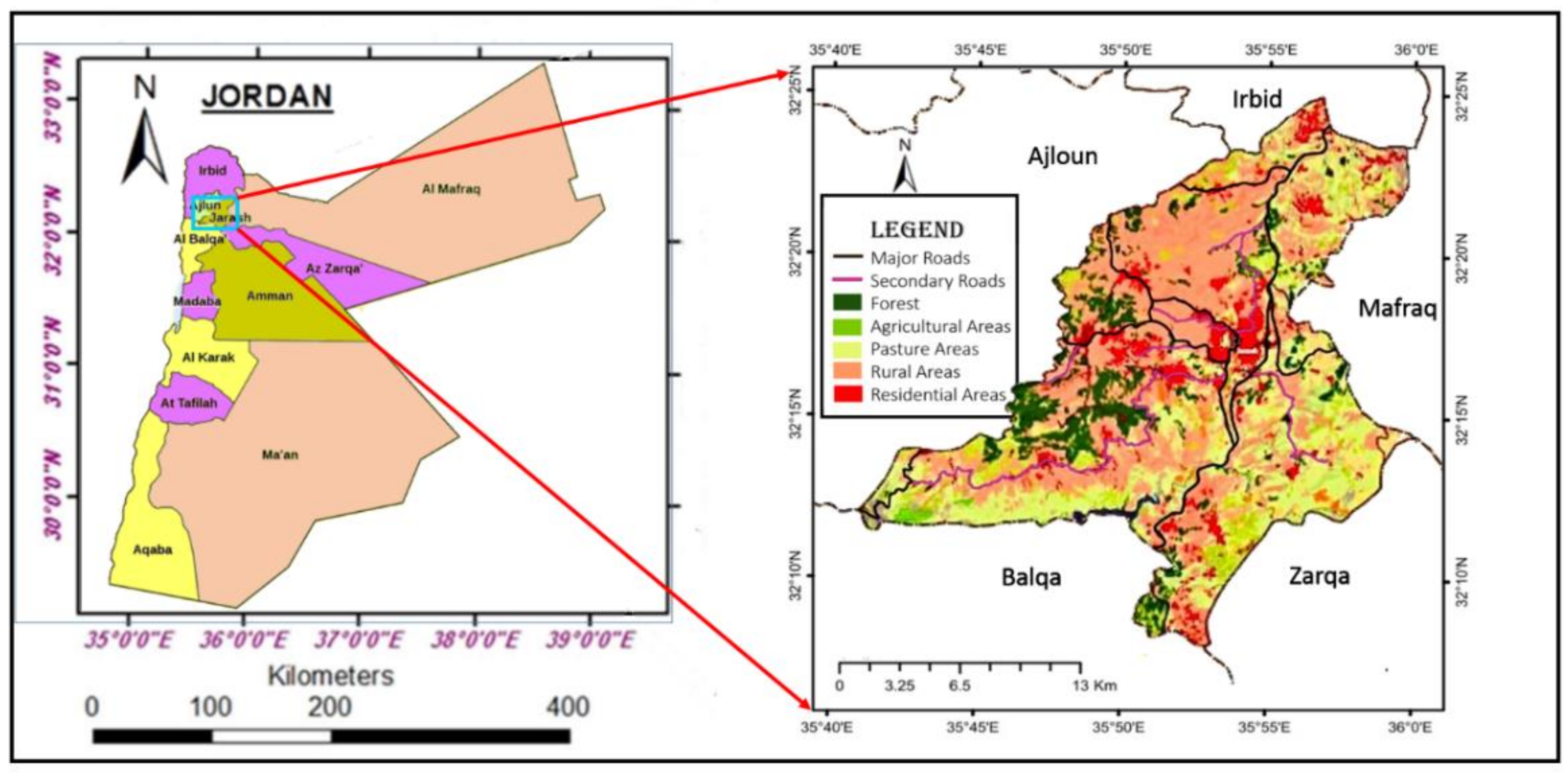
2.1. Study Area
2.2. Data Description
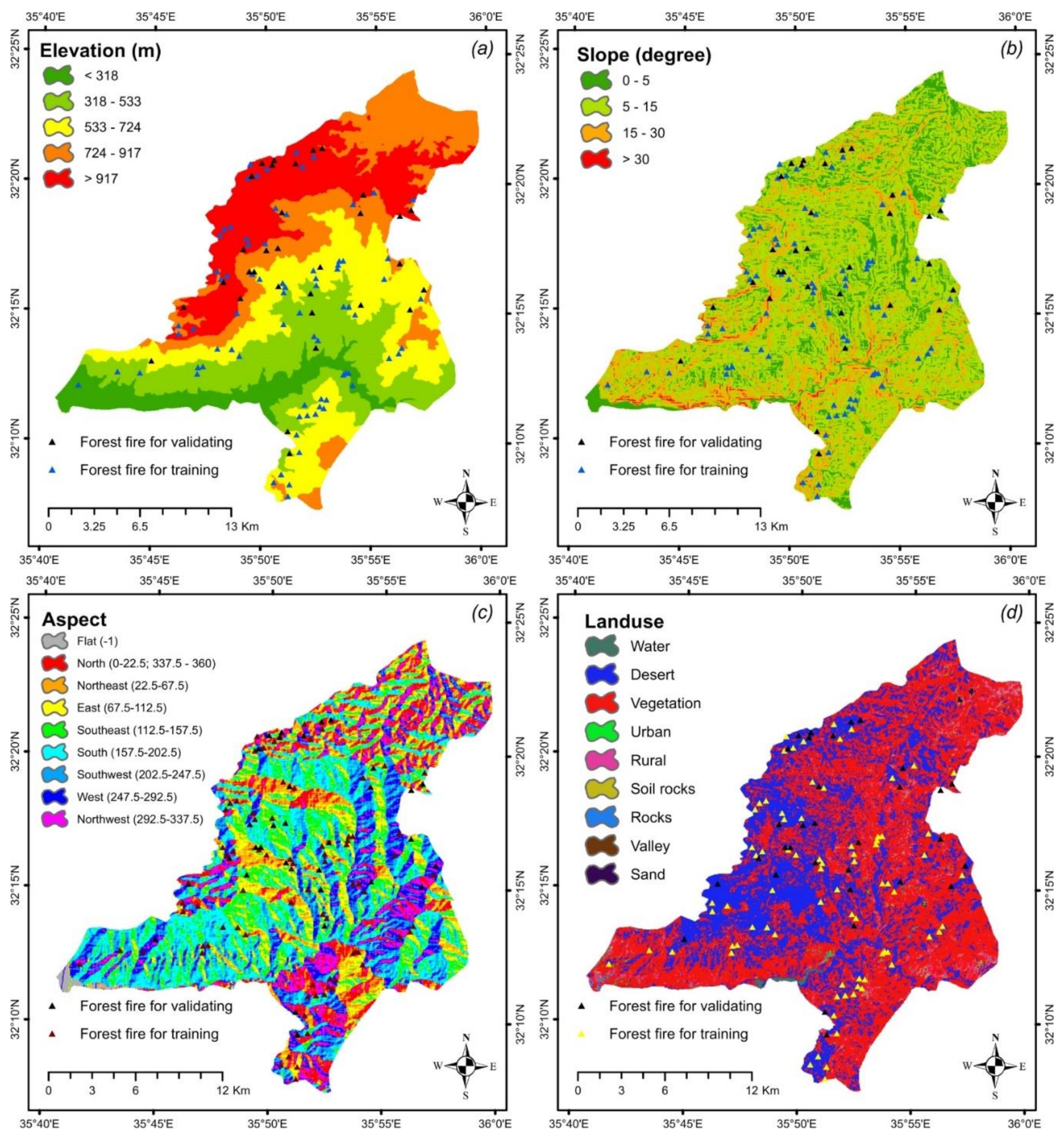
2.2.1. Elevation
2.2.2. Slope
2.2.3. Aspect
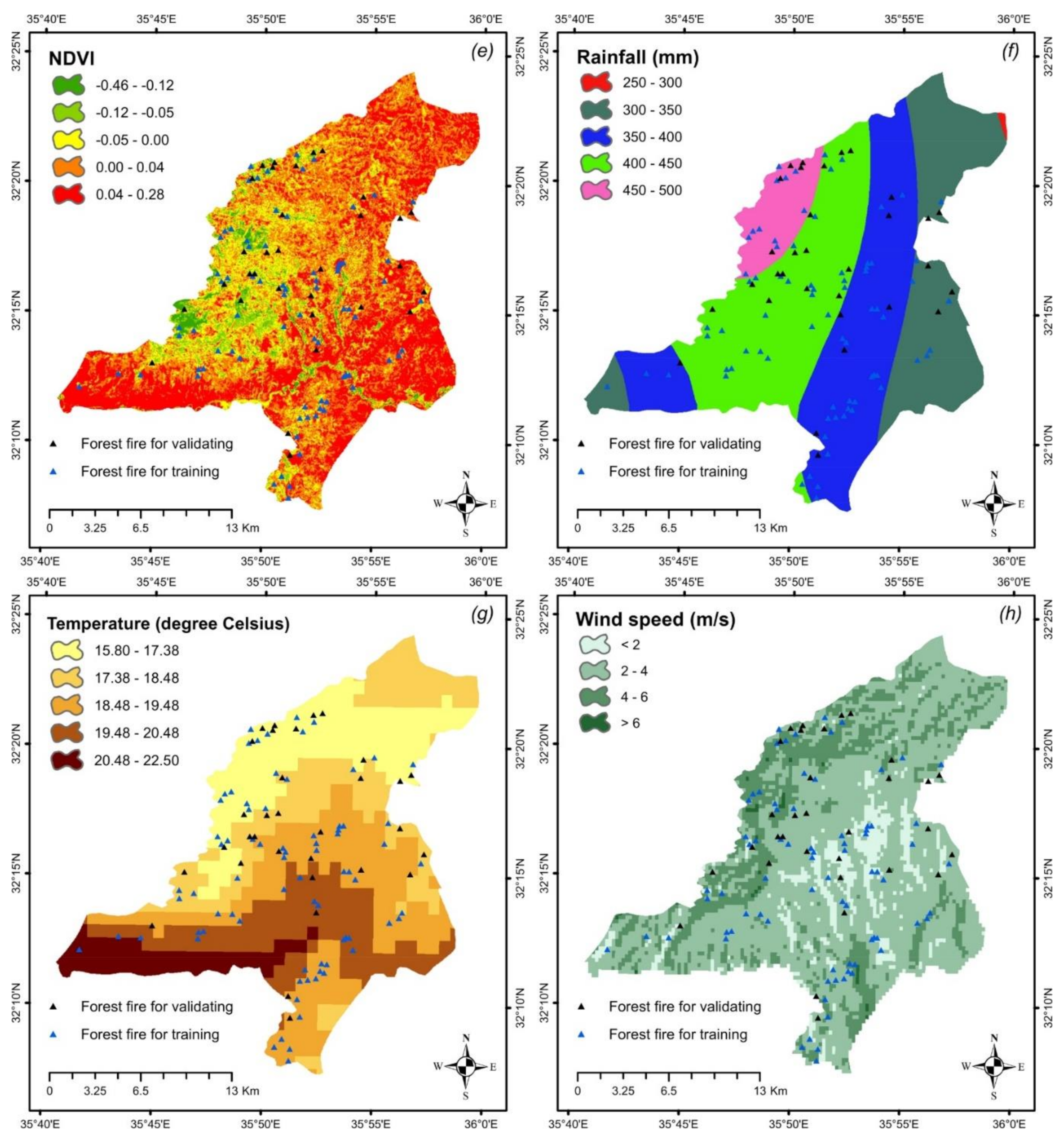
2.2.4. Wind Speed
2.2.5. TWI
2.2.6. Distance to Drainage
2.2.7. Temperature
2.2.8. Radiation
2.2.9. Rainfall
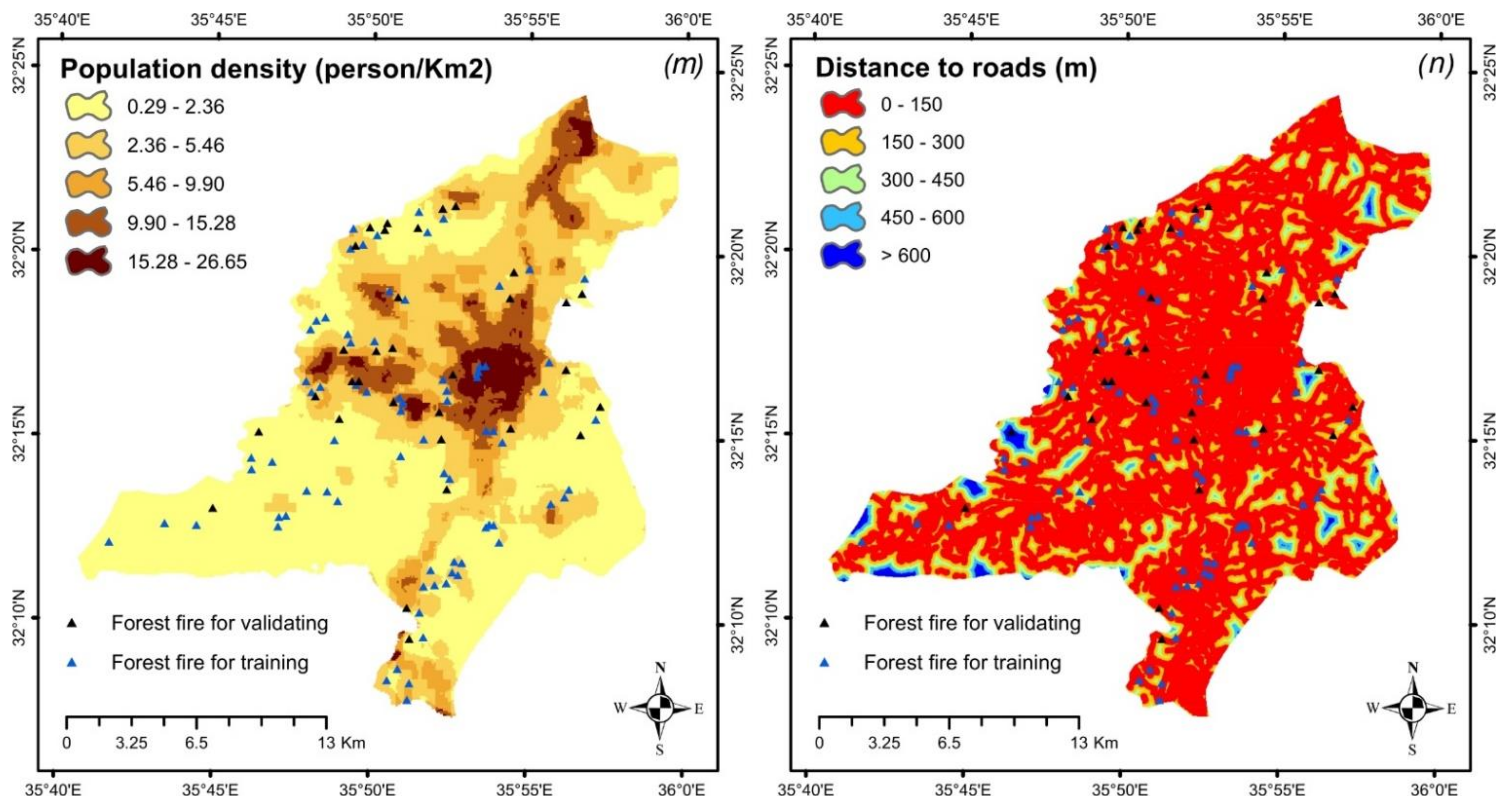
2.2.10. Population Density and Distance to Roads
2.2.11. Land Use Land Cover
2.2.12. NDVI
2.2.13. Soil Texture
3. Methodology
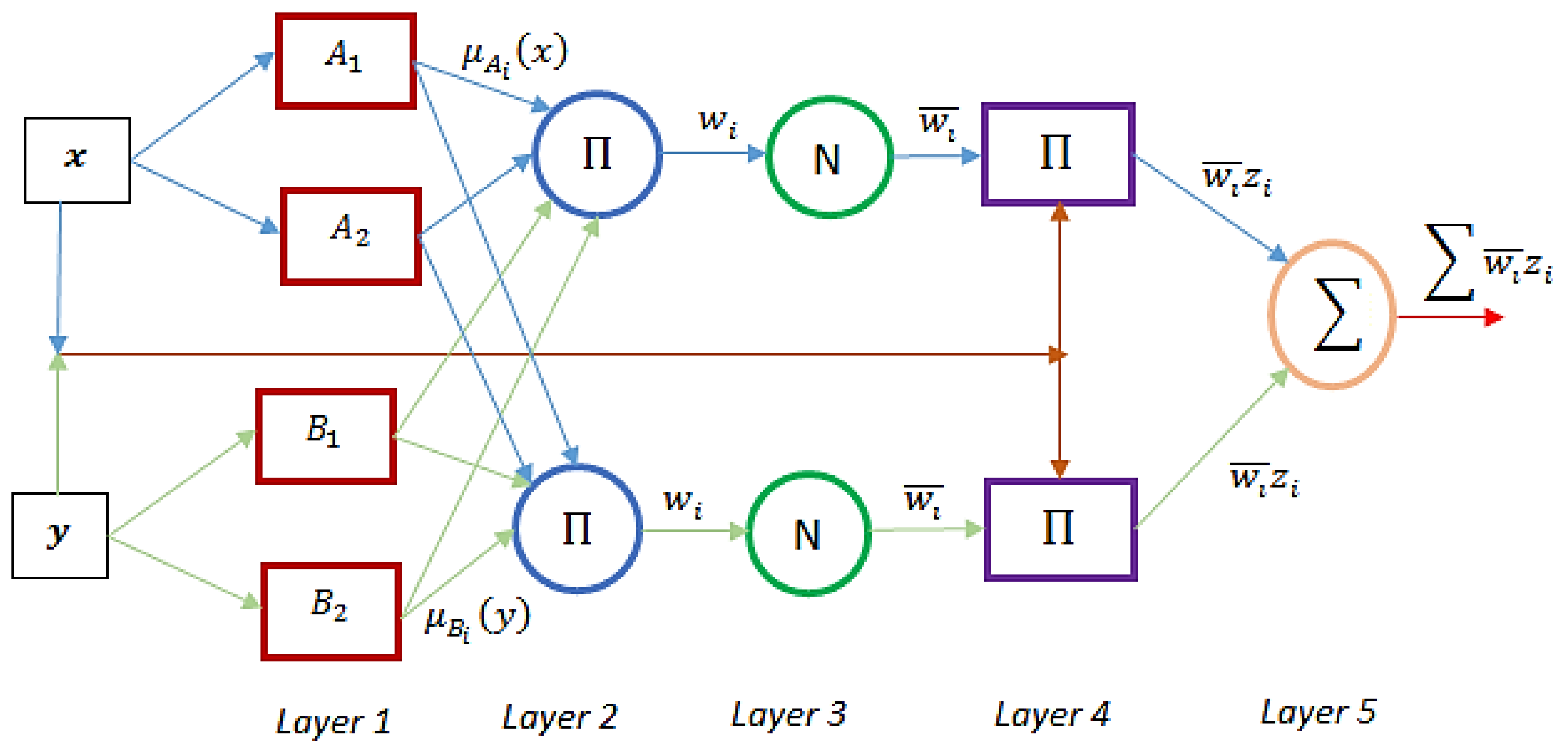
3.1. ANFIS
3.2. SVR
3.3. WOA
3.4. SA
3.5. Hybrid Models
3.6. Frequency Ratio (FR)
3.7. Feature Selection Process
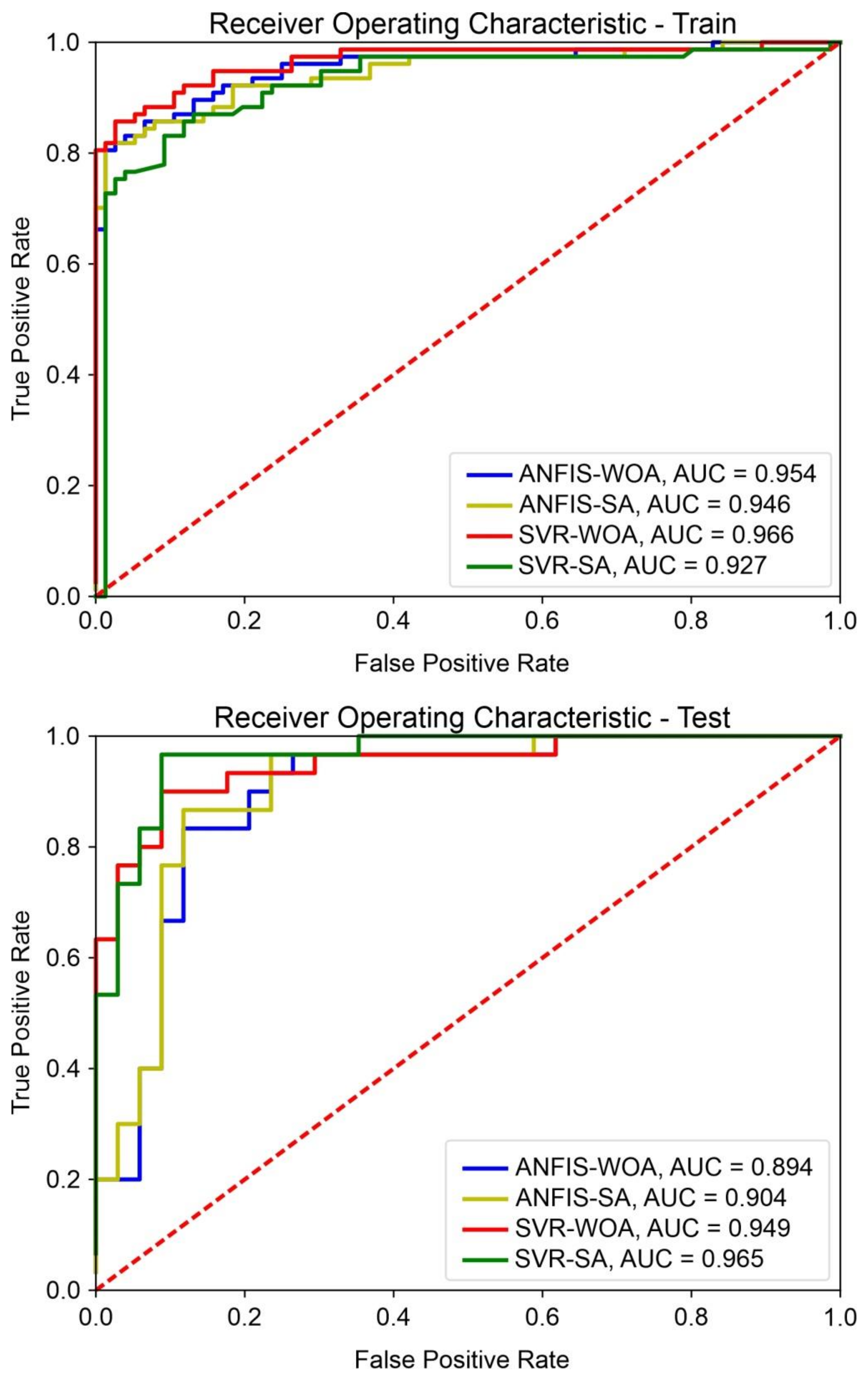
3.8. Relative Operating Characteristics (ROC)
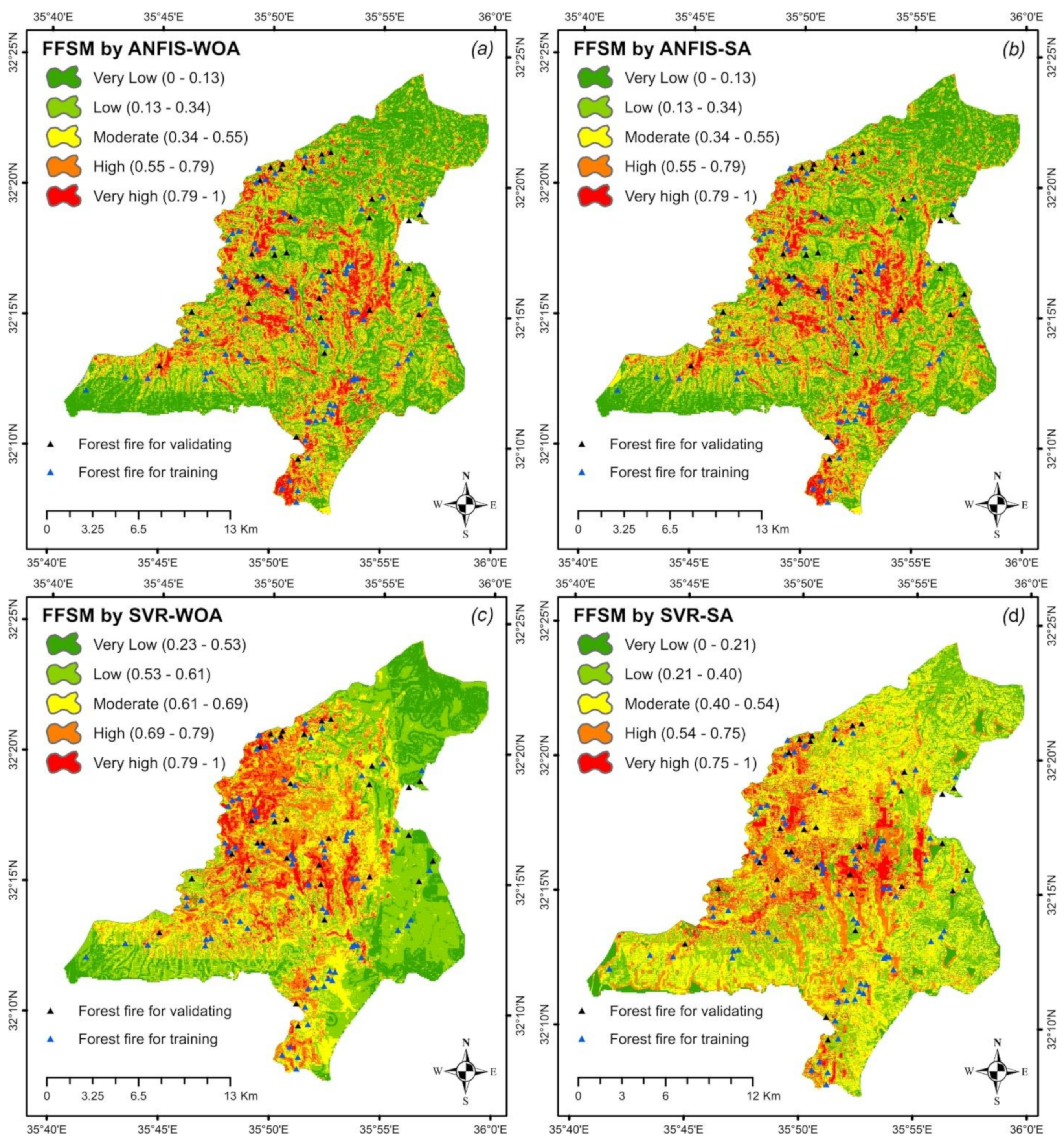
4. Results
5. Discussion
6. Conclusions
Author Contributions
Funding
Institutional Review Board Statement
Informed Consent Statement
Conflicts of Interest
References
- FAO; UNEP. The State of the World’s Forests. Forests, Biodiversity and People; FAO: Rome, Italy, 2020. [Google Scholar] [CrossRef]
- Chuvieco, E.; Allgöwer, B.; Salas, J. Integration of physical and human factors in fire danger assessment Wildland fire danger estimation and mapping: The role of remote sensing data. World Sci. 2003, 197–218. [Google Scholar] [CrossRef]
- Ganteaume, A.; Camia, A.; Jappiot, M.; San-Miguel-Ayanz, J.; Long-Fournel, M.; Lampin, C. A Review of the Main Driving Factors of Forest Fire Ignition Over Europe. Environ. Manag. 2013, 51, 651–662. [Google Scholar] [CrossRef] [PubMed] [Green Version]
- Abatzoglou, J.T.; Williams, A.P. Impact of anthropogenic climate change on wildfire across western US forests. Proc. Natl. Acad. Sci. USA 2016, 113, 11770–11775. [Google Scholar] [CrossRef] [Green Version]
- Masrur, A.; Petrov, A.N.; DeGroote, J. Circumpolar spatio-temporal patterns and contributing climatic factors of wildfire activity in the Arctic tundra from 2001–2015. Environ. Res. Lett. 2017, 13, 014019. [Google Scholar] [CrossRef] [Green Version]
- Özbayoğlu, A.M.; Bozer, R. Estimation of the Burned Area in Forest Fires Using Computational Intelligence Techniques. Procedia Comput. Sci. 2012, 12, 282–287. [Google Scholar] [CrossRef] [Green Version]
- Jaiswal, R.K.; Mukherjee, S.; Raju, K.D.; Saxena, R. Forest fire risk zone mapping from satellite imagery and GIS. Int. J. Appl. Earth Obs. Geoinf. 2002, 4, 1–10. [Google Scholar] [CrossRef]
- Vasilakos, C.; Kalabokidis, K.; Hatzopoulos, J.; Matsinos, I. Identifying wildland fire ignition factors through sensitivity analysis of a neural network. Nat. Hazards 2009, 50, 125–143. [Google Scholar] [CrossRef]
- Brown, J.K.; Smith, J.K. Wildland Fire in Ecosystems: Effects of Fire on Flora; General Technical Report RMRS-GTR-42-volume 2, Ogden, UT, USA; US Department of Agriculture, Forest Service, Rocky Mountain Research Station: Fort Collins, CO, USA, 2000; p. 42.
- Ozaki, V.A.; Goodwin, B.K.; Shirota, R. Parametric and nonparametric statistical modelling of crop yield: Implications for pricing crop insurance contracts. Appl. Econ. 2008, 40, 1151–1164. [Google Scholar] [CrossRef]
- Sheskin, D.J. Handbook of Parametric and Nonparametric Statistical Procedures, 5th ed.; CRC Press: Boca Raton, FL, USA, 2020. [Google Scholar] [CrossRef]
- Brownlee, J. Parametric and Non-Parametric Machine Learning Algorithms. Available online: http://machinelearningmastery.com/parametric-and-nonparametric-machinelearning-algorithms (accessed on 20 February 2021).
- Park, H.; Kim, N.; Lee, J. Parametric models and non-parametric machine learning models for predicting option prices: Empirical comparison study over KOSPI 200 Index options. Expert Syst. Appl. 2014, 41, 5227–5237. [Google Scholar] [CrossRef]
- Lehmann, E.L. Parametric Versus Nonparametrics: Two Alternative Methodologies; Selected Works of EL Lehmann; Springer: Berlin/Heidelberg, Germany, 2012; pp. 437–445. [Google Scholar]
- Samui, P. Support vector machine applied to settlement of shallow foundations on cohesionless soils. Comput. Geotech. 2008, 35, 419–427. [Google Scholar] [CrossRef]
- Auret, L.; Aldrich, C. Interpretation of nonlinear relationships between process variables by use of random forests. Miner. Eng. 2012, 35, 27–42. [Google Scholar] [CrossRef]
- Ahmadlou, M.; Al-Fugara, A.k.; Al-Shabeeb, A.R.; Arora, A.; Al-Adamat, R.; Pham, Q.B.; Al-Ansari, N.; Linh, N.T.T.; Sajedi, H. Flood susceptibility mapping and assessment using a novel deep learning model combining multilayer perceptron and autoencoder neural networks. J. Flood Risk Manag. 2021, 14, e12683. [Google Scholar] [CrossRef]
- Bui, Q.-T.; Nguyen, Q.-H.; Nguyen, X.L.; Pham, V.D.; Nguyen, H.D.; Pham, V.-M. Verification of novel integrations of swarm intelligence algorithms into deep learning neural network for flood susceptibility mapping. J. Hydrol. 2020, 581, 124379. [Google Scholar] [CrossRef]
- Chao, L.; Zhang, K.; Li, Z.; Zhu, Y.; Wang, J.; Yu, Z. Geographically weighted regression based methods for merging satellite and gauge precipitation. J. Hydrol. 2018, 558, 275–289. [Google Scholar] [CrossRef]
- Chen, Y.; Zheng, W.; Li, W.; Huang, Y. Large group activity security risk assessment and risk early warning based on random forest algorithm. Pattern Recognit. Lett. 2021, 144, 1–5. [Google Scholar] [CrossRef]
- Gao, N.; Luo, D.; Cheng, B.; Hou, H. Teaching-learning-based optimization of a composite metastructure in the 0–10 kHz broadband sound absorption range. J. Acoust. Soc. Am. 2020, 148, EL125–EL129. [Google Scholar] [CrossRef] [PubMed]
- Wang, J.; Zhu, P.; He, B.; Deng, G.; Zhang, C.; Huang, X. An Adaptive Neural Sliding Mode Control with ESO for Uncertain Nonlinear Systems. Int. J. Control. Autom. Syst. 2021, 19, 687–697. [Google Scholar] [CrossRef]
- Zhang, K.; Zhang, J.; Ma, X.; Yao, C.; Zhang, L.; Yang, Y.; Wang, J.; Yao, J.; Zhao, H. History Matching of Naturally Fractured Reservoirs Using a Deep Sparse Autoencoder. SPE J. 2021, 1–22. [Google Scholar] [CrossRef]
- Ahmadlou, M.; Karimi, M.; Alizadeh, S.; Shirzadi, A.; Parvinnejhad, D.; Shahabi, H.; Panahi, M. Flood susceptibility assessment using integration of adaptive network-based fuzzy inference system (ANFIS) and biogeography-based optimization (BBO) and BAT algorithms (BA). Geocarto Int. 2019, 34, 1252–1272. [Google Scholar] [CrossRef]
- Zhao, G.; Pang, B.; Xu, Z.; Peng, D.; Xu, L. Assessment of urban flood susceptibility using semi-supervised machine learning model. Sci. Total Environ. 2019, 659, 940–949. [Google Scholar] [CrossRef] [PubMed]
- Al-Fugara, A.; Ahmadlou, M.; Al-Shabeeb, A.R.; Alayyash, S.; Al-Amoush, H.; Al-Adamat, R. Spatial mapping of groundwater springs potentiality using grid search-based and genetic algorithm-based support vector regression. Geocarto Int. 2020, 1–20. [Google Scholar] [CrossRef]
- Al-Fugara, A.; Ahmadlou, M.; Shatnawi, R.; Alayyash, S.; Al-Adamat, R.; Al-Shabeeb, A.A.-R.; Soni, S. Novel hybrid models combining meta-heuristic algorithms with support vector regression (SVR) for groundwater potential mapping. Geocarto Int. 2020, 1–20. [Google Scholar] [CrossRef]
- Kumar, T.; Gautam, A.K.; Kumar, T. Appraising the accuracy of GIS-based multi-criteria decision making technique for delineation of groundwater potential zones. Water Resour. Manag. 2014, 28, 4449–4466. [Google Scholar] [CrossRef]
- Sachdeva, S.; Bhatia, T.; Verma, A.K. GIS-based evolutionary optimized Gradient Boosted Decision Trees for forest fire susceptibility mapping. Nat. Hazards 2018, 92, 1399–1418. [Google Scholar] [CrossRef]
- Bisquert, M.; Caselles, E.; Sánchez, J.M.; Caselles, V. Application of artificial neural networks and logistic regression to the prediction of forest fire danger in Galicia using MODIS data. Int. J. Wildland Fire 2012, 21, 1025–1029. [Google Scholar] [CrossRef]
- USGS. Shuttle Radar Topography Mission. Available online: https://earthexplorer.usgs.gov (accessed on 25 December 2018).
- Zhang, Z.; Luo, C.; Zhao, Z. Application of probabilistic method in maximum tsunami height prediction considering stochastic seabed topography. Nat. Hazards 2020, 104, 2511–2530. [Google Scholar] [CrossRef]
- Ertena, E.; Kurgun, V.; Musaoglu, N. Forest fire risk zone mapping from satellite imagery and GIS: A case study. In Proceedings of the XXth Congress of the International Society for Photogrammetry and Remote Sensing, Istanbul, Turkey, 12–23 July 2004; pp. 222–230. [Google Scholar]
- Ireland, G.; Petropoulos, G.P. Exploring the relationships between post-fire vegetation regeneration dynamics, topography and burn severity: A case study from the Montane Cordillera Ecozones of Western Canada. Appl. Geogr. 2015, 56, 232–248. [Google Scholar] [CrossRef]
- Ramos-Neto, M.B.; Pivello, V.R. Lightning Fires in a Brazilian Savanna National Park: Rethinking Management Strategies. Environ. Manag. 2000, 26, 675–684. [Google Scholar] [CrossRef] [PubMed]
- Renard, Q.; Pélissier, R.; Ramesh, B.R.; Kodandapani, N. Environmental susceptibility model for predicting forest fire occurrence in the Western Ghats of India. Int. J. Wildland Fire 2012, 21, 368–379. [Google Scholar] [CrossRef] [Green Version]
- Moore, I.D.; Grayson, R.B.; Ladson, A.R. Digital terrain modelling: A review of hydrological, geomorphological, and biological applications. Hydrol. Process. 1991, 5, 3–30. [Google Scholar] [CrossRef]
- Martinez, J.; Vega-Garcia, C.; Chuvieco, E. Human-caused wildre risk rating for prevention planning in Spain. J. Environ. Manag. 2009, 90, 1241–1252. [Google Scholar] [CrossRef]
- Ganteaume, A.; Marielle, J.; Corinne, L.-M.; Thomas, C.; Laurent, B. Effects of vegetation type and fire regime on flammability of undisturbed litter in Southeastern France. For. Ecol. Manag. 2011, 261, 2223–2231. [Google Scholar] [CrossRef]
- Glovis. USGS Global Visualization Viewer. 2018. Available online: http://glovis.usgs.gov (accessed on 25 December 2018).
- Jensen, J.R. Introductory Digital Image Processing A Remote Sensing Perspective Second Edition; Pearson: Hoboken, NJ, USA, 1995; ISBN 978-0-13-205840-7. [Google Scholar]
- Jang, J.-S. ANFIS: Adaptive-network-based fuzzy inference system. IEEE Trans. Syst. Mancybern. 1993, 23, 665–685. [Google Scholar] [CrossRef]
- Bergsten, P.; Palm, R.; Driankov, D. Observers for Takagi-Sugeno fuzzy systems. IEEE Trans. Syst. Mancybern. Part B 2002, 32, 114–121. [Google Scholar] [CrossRef] [PubMed]
- Gill, J.; Singh, J. Energetic and exergetic performance analysis of the vapor compression refrigeration system using adaptive neuro-fuzzy inference system approach. Exp. Therm. Fluid Sci. 2017, 88, 246–260. [Google Scholar] [CrossRef]
- Walia, N.; Singh, H.; Sharma, A. ANFIS: Adaptive Neuro-Fuzzy Inference System- A Survey. Int. J. Comput. Appl. 2015, 123, 32–38. [Google Scholar] [CrossRef]
- Awad, M.; Khanna, R. Support Vector Regression Efficient Learning Machines; Springer: Berlin/Heidelberg, Germany, 2015; pp. 67–80. [Google Scholar]
- Drucker, H.; Surges, C.J.C.; Kaufman, L.; Smola, A.; Vapnik, V. Support vector regression machines. Adv. Neural Inf. Process. Syst. 1997, 1, 155–161. [Google Scholar]
- Peng, H.; Ling, X. Predicting thermal–hydraulic performances in compact heat exchangers by support vector regression. Int. J. Heat Mass Transf. 2015, 84, 203–213. [Google Scholar] [CrossRef]
- Zaidi, S. Novel application of support vector machines to model the two phase boiling heat transfer coefficient in a vertical tube thermosiphon reboiler. Chem. Eng. Res. Des. 2015, 98, 44–58. [Google Scholar] [CrossRef]
- Belegundu, A.D.; Chandrupatla, T.R. Optimization Concepts and Applications in Engineering; Cambridge University Press: Cambridge, UK, 2019. [Google Scholar]
- Ma, X.; Zhang, K.; Zhang, L.; Yao, C.; Yao, J.; Wang, H.; Jian, W.; Yan, Y. Data-Driven Niching Differential Evolution with Adaptive Parameters Control for History Matching and Uncertainty Quantification. SPE J. 2021, 26, 993–1010. [Google Scholar] [CrossRef]
- Zhao, J.; Liu, J.; Jiang, J.; Gao, F. Efficient Deployment with Geometric Analysis for mmWave UAV Communications. IEEE Wirel. Commun. Lett. 2020, 9, 1115–1119. [Google Scholar] [CrossRef]
- Deng, Y.; Zhang, T.; Sharma, B.K.; Nie, H. Optimization and mechanism studies on cell disruption and phosphorus recovery from microalgae with magnesium modified hydrochar in assisted hydrothermal system. Sci. Total Environ. 2019, 646, 1140–1154. [Google Scholar] [CrossRef] [PubMed]
- Jiang, Q.; Shao, F.; Lin, W.; Gu, K.; Jiang, G.; Sun, H. Optimizing Multistage Discriminative Dictionaries for Blind Image Quality Assessment. IEEE Trans. Multimed. 2018, 20, 2035–2048. [Google Scholar] [CrossRef]
- Xue, X.; Zhang, K.; Tan, K.C.; Feng, L.; Wang, J.; Chen, G.; Zhao, X.; Zhang, L.; Yao, J. Affine Transformation-Enhanced Multifactorial Optimization for Heterogeneous Problems. IEEE Trans. Cybern. 2020, 1–15. [Google Scholar] [CrossRef] [PubMed]
- Zhou, Y.; Tian, L.; Zhu, C.; Jin, X.; Sun, Y. Video Coding Optimization for Virtual Reality 360-Degree Source. IEEE J. Sel. Top. Signal Process. 2020, 14, 118–129. [Google Scholar] [CrossRef]
- Mirjalili, S.; Lewis, A. The Whale Optimization Algorithm. Adv. Eng. Softw. 2016, 95, 51–67. [Google Scholar] [CrossRef]
- Kirkpatrick, S.; Gelatt, C.D.; Vecchi, M.P. Optimization by Simulated Annealing. Science 1983, 220, 671–680. [Google Scholar] [CrossRef] [PubMed]
- Van Laarhoven, P.J.; Aarts, E.H. Simulated Annealing: Theory and Applications; Springer: Berlin/Heidelberg, Germany, 1987; pp. 7–15. [Google Scholar]
- Davis, L. Genetic Algorithms and Simulated Annealing; Morgan Kaufmann Publishers: Burlington, MA, USA, 1987. [Google Scholar]
- Selim, S.Z.; Alsultan, K. A simulated annealing algorithm for the clustering problem. Pattern Recognit. 1991, 24, 1003–1008. [Google Scholar] [CrossRef]
- Fengjie, S.; He, W.; Jieqing, F. 2D Otsu Segmentation Algorithm Based on Simulated Annealing Genetic Algorithm for Iced-Cable Images. In Proceedings of the 2009 Information Technology and Applications, Chengdu, China, 15–17 May 2009; pp. 600–602. [Google Scholar] [CrossRef]
- Li, L.; Lan, H.; Guo, C.; Zhang, Y.; Li, Q.; Wu, Y. A modified frequency ratio method for landslide susceptibility assessment. Landslides 2017, 14, 727–741. [Google Scholar] [CrossRef]
- Zenggang, X.; Zhiwen, T.; Xiaowen, C.; Xue-min, Z.; Kaibin, Z.; Conghuan, Y. Research on image retrieval algorithm based on combination of color and shape features. J. Signal Process. Syst. 2019, 93, 1–8. [Google Scholar] [CrossRef]
- Mason, S.J.; Graham, N.E. Areas beneath the relative operating characteristics (ROC) and relative operating levels (ROL) curves: Statistical significance and interpretation. Q. J. R. Meteorol. Soc. 2002, 128, 2145–2166. [Google Scholar] [CrossRef]
- Boyd, K.; Eng, K.H.; Page, C.D. Area under the precision-recall curve: Point estimates and confidence intervals. In Proceedings of the Joint European Conference on Machine Learning and Knowledge Discovery in Databases, Prague, Czech Republic, 23–27 September 2013; Springer: Berlin/Heidelberg, Germany, 2013; pp. 451–466. [Google Scholar]
- Shafizadeh-Moghadam, H.; Tayyebi, A.; Ahmadlou, M.; Delavar, M.R.; Hasanlou, M. Integration of genetic algorithm and multiple kernel support vector regression for modeling urban growth. Comput. Environ. Urban Syst. 2017, 65, 28–40. [Google Scholar] [CrossRef]
- He, Z.; Wen, X.; Liu, H.; Du, J. A comparative study of artificial neural network, adaptive neuro fuzzy inference system and support vector machine for forecasting river flow in the semiarid mountain region. J. Hydrol. 2014, 509, 379–386. [Google Scholar] [CrossRef]
- Hipni, A.; El-Shafie, A.; Najah, A.; Karim, O.A.; Hussain, A.; Mukhlisin, M. Daily Forecasting of Dam Water Levels: Comparing a Support Vector Machine (SVM) Model With Adaptive Neuro Fuzzy Inference System (ANFIS). Water Resour. Manag. 2013, 27, 3803–3823. [Google Scholar] [CrossRef]
- Adab, H.; Kanniah, K.D.; Solaimani, K.; Sallehuddin, R. Modelling static fire hazard in a semi-arid region using frequency analysis. Int. J. Wildland Fire 2015, 24, 763–777. [Google Scholar] [CrossRef]
- Chen, F.; Du, Y.; Niu, S.; Zhao, J. Modeling Forest Lightning Fire Occurrence in the Daxinganling Mountains of Northeastern China with MAXENT. Forests 2015, 6, 1422–1438. [Google Scholar] [CrossRef] [Green Version]
- Oliveira, S.; Pereira, J.M.; San-Miguel-Ayanz, J.; Lourenço, L. Exploring the spatial patterns of fire density in Southern Europe using Geographically Weighted Regression. Appl. Geogr. 2014, 51, 143–157. [Google Scholar] [CrossRef]
- Eskandari, S.; Miesel, J.R. Comparison of the fuzzy AHP method, the spatial correlation method, and the Dong model to predict the re high-risk areas in Hyrcanian forests of Iran. Geomat. Nat. Hazards Risk 2017, 8, 933–949. [Google Scholar] [CrossRef] [Green Version]
- Zaghloul, M.S.; Hamza, R.A.; Iorhemen, O.T.; Tay, J.H. Comparison of adaptive neuro-fuzzy inference systems (ANFIS) and support vector regression (SVR) for data-driven modelling of aerobic granular sludge reactors. J. Environ. Chem. Eng. 2020, 8, 103742. [Google Scholar] [CrossRef]


| Model | |||
|---|---|---|---|
| Reality | Positive | Negative | |
| Positive | True Positive (TP) | False Negative (FN) | |
| Negative | False Positive (FP) | True Negative (TN) | |
| Factors | Classes | No. of Pixels | No. of Fires | FR Weights |
|---|---|---|---|---|
| Elevation (m) | <318 | 40,604 | 4 | 0.57 |
| 318–533 | 100,277 | 13 | 0.75 | |
| 533–724 | 113,580 | 32 | 1.63 | |
| 724–917 | 98,876 | 10 | 0.59 | |
| >917 | 94,337 | 18 | 1.11 | |
| Aspect | Flat | 3155 | 0 | 0 |
| North | 45,764 | 4 | 0.51 | |
| Northeast | 40,550 | 16 | 2.29 | |
| East | 57,810 | 12 | 1.21 | |
| Southeast | 68,725 | 5 | 0.42 | |
| South | 86,407 | 12 | 0.8 | |
| Southeast | 55,591 | 9 | 0.94 | |
| West | 52,336 | 14 | 1.56 | |
| Northwest | 37,333 | 5 | 0.78 | |
| Slope | 0–5 | 81,146 | 11 | 0.79 |
| 5–15 | 267,384 | 44 | 0.96 | |
| 15–30 | 92,246 | 22 | 1.39 | |
| >30 | 6895 | 0 | 0 | |
| Rainfall | 300–350 | 113,527 | 8 | 0.41 |
| 350–400 | 154,167 | 30 | 1.13 | |
| 250–300 | 721 | 0 | 0 | |
| 400–450 | 145,311 | 28 | 1.12 | |
| 450–500 | 33,945 | 11 | 1.88 | |
| NDVI | −0.46–−0.12 | 9921 | 4 | 2.34 |
| −0.12–−0.05 | 30,689 | 16 | 3.03 | |
| −0.05–0.00 | 87,641 | 22 | 1.5 | |
| 0.00–0.04 | 164,081 | 23 | 0.81 | |
| 0.04–0.28 | 155,339 | 12 | 0.45 | |
| TWI | <9 | 121,081 | 27 | 1.3 |
| 9–13 | 217,055 | 32 | 0.86 | |
| >13 | 109,535 | 18 | 0.96 | |
| Distance to rivers | 0–150 | 133,092 | 22 | 0.96 |
| 150–300 | 107,127 | 20 | 1.09 | |
| 300–450 | 87,220 | 9 | 0.6 | |
| 450–600 | 60,126 | 12 | 1.16 | |
| >600 | 60,106 | 14 | 1.35 | |
| Temperature (C) | 15.80–17.38 | 102,494 | 19 | 1.08 |
| 17.38–18.48 | 101,010 | 10 | 0.58 | |
| 18.48–19.48 | 122,338 | 34 | 1.62 | |
| 19.48–20.48 | 85,621 | 13 | 0.88 | |
| 20.48–22.50 | 36,208 | 1 | 0.16 | |
| Distance to roads | 0–150 | 336,475 | 67 | 1.16 |
| 150–300 | 77,584 | 7 | 0.52 | |
| 300–450 | 23,018 | 3 | 0.76 | |
| 450–600 | 7010 | 0 | 0 | |
| >600 | 3584 | 0 | 0 | |
| Wind speed (m/s) | <2 | 44,027 | 14 | 1.83 |
| 2–4 | 297,820 | 45 | 0.87 | |
| 4–6 | 99,681 | 17 | 0.98 | |
| >6 | 2231 | 1 | 2.58 | |
| LULC | Water | 1612 | 0 | 0 |
| Bare soil | 159,679 | 48 | 1.75 | |
| Vegetation | 256,798 | 25 | 0.57 | |
| Urban | 2020 | 2 | 5.76 | |
| Rural | 20,120 | 1 | 0.29 | |
| Soil rocks | 3953 | 0 | 0 | |
| Rocks | 1049 | 0 | 0 | |
| Valley | 1296 | 0 | 0 | |
| Sand | 1144 | 1 | 5.08 | |
| Radiation (watt/m2) | 5.43–5.64 | 18,272 | 3 | 0.95 |
| 5.64–5.70 | 81,265 | 17 | 1.22 | |
| 5.70–5.75 | 180,178 | 43 | 1.39 | |
| 5.75–5.82 | 167,956 | 14 | 0.48 | |
| Soil texture | Loam | 4698 | 1 | 1.24 |
| Silty Clay | 481 | 0 | 0 | |
| Silty Loam | 261,932 | 44 | 0.98 | |
| Clay Loam | 180,560 | 32 | 1.03 | |
| Population density | 0.29–2.36 | 227,182 | 31 | 0.79 |
| (person/km2) | 2.36–5.46 | 124,104 | 26 | 1.22 |
| 5.46–9.90 | 413,38 | 8 | 1.13 | |
| 9.90–15.28 | 39,838 | 11 | 1.61 | |
| 15.28–26.65 | 15,209 | 1 | 0.38 |
| Explanatory Variables | SVR-SA | SVR-WOA | ANFIS-SA | ANFIS-WOA |
|---|---|---|---|---|
| Elevation | ☑ | ☑ | ☑ | ☑ |
| Slope aspect | ☑ | - | - | - |
| Slope | ☑ | ☑ | ☑ | ☑ |
| Land use | ☑ | - | ☑ | ☑ |
| TWI | ☑ | ☑ | ☑ | ☑ |
| NDVI | ☑ | ☑ | ☑ | ☑ |
| Distance to drainage | ☑ | ☑ | ☑ | ☑ |
| Distance to roads | - | - | - | - |
| Soil texture | - | - | ☑ | - |
| Wind speed | - | ☑ | - | ☑ |
| Solar radiation | ☑ | ☑ | ☑ | ☑ |
| Rainfall | ☑ | ☑ | ☑ | ☑ |
| Temperature | ☑ | ☑ | ☑ | ☑ |
| Population density | ☑ | ☑ | ☑ | ☑ |
| Land Use Class | Pixel No. |
|---|---|
| Water | 0 (0.00%) |
| Bare soil | 67,614 (55.23%) |
| Vegetation | 50,032 (40.87%) |
| Urban | 387 (0.32%) |
| Rural | 3117 (2.55%) |
| Soil | 552 (0.45%) |
| Rocks | 67 (0.05%) |
| Valley | 143 (0.12%) |
| Sand | 183 (0.15%) |
Publisher’s Note: MDPI stays neutral with regard to jurisdictional claims in published maps and institutional affiliations. |
© 2021 by the authors. Licensee MDPI, Basel, Switzerland. This article is an open access article distributed under the terms and conditions of the Creative Commons Attribution (CC BY) license (https://creativecommons.org/licenses/by/4.0/).
Share and Cite
Al-Fugara, A.; Mabdeh, A.N.; Ahmadlou, M.; Pourghasemi, H.R.; Al-Adamat, R.; Pradhan, B.; Al-Shabeeb, A.R. Wildland Fire Susceptibility Mapping Using Support Vector Regression and Adaptive Neuro-Fuzzy Inference System-Based Whale Optimization Algorithm and Simulated Annealing. ISPRS Int. J. Geo-Inf. 2021, 10, 382. https://doi.org/10.3390/ijgi10060382
Al-Fugara A, Mabdeh AN, Ahmadlou M, Pourghasemi HR, Al-Adamat R, Pradhan B, Al-Shabeeb AR. Wildland Fire Susceptibility Mapping Using Support Vector Regression and Adaptive Neuro-Fuzzy Inference System-Based Whale Optimization Algorithm and Simulated Annealing. ISPRS International Journal of Geo-Information. 2021; 10(6):382. https://doi.org/10.3390/ijgi10060382
Chicago/Turabian StyleAl-Fugara, A’kif, Ali Nouh Mabdeh, Mohammad Ahmadlou, Hamid Reza Pourghasemi, Rida Al-Adamat, Biswajeet Pradhan, and Abdel Rahman Al-Shabeeb. 2021. "Wildland Fire Susceptibility Mapping Using Support Vector Regression and Adaptive Neuro-Fuzzy Inference System-Based Whale Optimization Algorithm and Simulated Annealing" ISPRS International Journal of Geo-Information 10, no. 6: 382. https://doi.org/10.3390/ijgi10060382