Article

Quest for Optimal Regression Models in SARS-CoV-2 Wastewater Based Epidemiology

1
Department of Infrastructure, University Innsbruck, 6020 Innsbruck, Austria
2
Department of Microbiology, University Innsbruck, 6020 Innsbruck, Austria
3
Institute for Water Quality and Resource Management, Technology University Vienna, 1040 Vienna, Austria
*
Author to whom correspondence should be addressed.
Int. J. Environ. Res. Public Health 2021, 18(20), 10778; https://doi.org/10.3390/ijerph182010778
Submission received: 11 September 2021 / Revised: 5 October 2021 / Accepted: 9 October 2021 / Published: 14 October 2021
(This article belongs to the Topic Wastewater-Based Epidemiology)

Abstract

:
Wastewater-based epidemiology is a recognised source of information for pandemic management. In this study, we investigated the correlation between a SARS-CoV-2 signal derived from wastewater sampling and COVID-19 incidence values monitored by means of individual testing programs. The dataset used in the study is composed of timelines (duration approx. five months) of both signals at four wastewater treatment plants across Austria, two of which drain large communities and the other two drain smaller communities. Eight regression models were investigated to predict the viral incidence under varying data inputs and pre-processing methods. It was found that population-based normalisation and smoothing as a pre-processing of the viral load data significantly influence the fitness of the regression models. Moreover, the time latency lag between the wastewater data and the incidence derived from the testing program was found to vary between 2 and 7 days depending on the time period and site. It was found to be necessary to take such a time lag into account by means of multivariate modelling to boost the performance of the regression. Comparing the models, no outstanding one could be identified as all investigated models are revealing a sufficient correlation for the task. The pre-processing of data and a multivariate model formulation is more important than the model structure.

1. Introduction

For decades, data collected from the inflow of wastewater treatment plants (WWTPs) have been recognised as an important source of information for the detection of human diseases and/or drug abuse [1,2,3,4]. Consequently, for the Sars-Cov-2 pandemic as well, multiple studies have found wastewater-based epidemiology (WBE) as a potential tool [5,6,7,8,9,10] for the monitoring and management of the disease. The virus signal found in wastewater is the true prevalence information, that is, information on all infected persons in the watershed [11,12,13,14]. However, official reporting and statistics relies on the data derived from individual test programs, which includes only a subset of the overall infection and is a function of the test strategy. The difference to the true number of infections (as determined by prevalence data) is significant due to the high number of asymptomatic and mildly infected patients [15]. Still, the latter information serves as the backbone of SARS-CoV-2 management and is usually denoted as the incidence value, typically given as the 7- or 14-day notification rate of new infections for 100,000 inhabitants.
Despite the differences in the properties of the data (WBE prevalence and test-based incidence), studies have reported a significant statistical agreement between the two [16,17], thus indicating the capability of wastewater data for the prediction of COVID-19 incidence data [18]. In terms of pandemic management, this is a profound advantage both as supplement and alternative to individual testing. Furthermore, WBE was found to give a slightly earlier signal as compared to the clinical recognition of SARS-CoV-2 [19,20,21]. Thus, a mathematical model capable to predict the incidence values from the wastewater signal is a valuable tool in pandemic management.
Whereas a simple statistical model, such as a linear regression, can correlate two signals, a thorough analysis of the mechanisms and assumptions of the models are key for a robust prediction [22,23]. For instance, in addition to the observed latency between two signals, it was shown that the inclusion of metadata on the amount of testing might have a positive effect on the model performance. It is evident that increasing the number of tests results in the identification of a higher number of positive cases. However, owing to a lack of comprehensive community monitoring [24,25,26]; untested asymptomatic individuals, who comprise a significant number of patients [27,28,29,30,31]; and data security concerns, detailed test data—allowing for prevalence estimation—is unavailable on a general basis, thereby restricting the development of rigorous statistical models.
In relation to WBE modelling, researchers have taken advantage of regression models as a powerful technique for predicting and identifying the use and spread of substances in the population [32,33]. Regarding COVID-19, [10,34,35,36,37,38,39] published statistical models for the prediction of the number of active cases based on clinical information. However, only a few studies were dedicated to the regression between the viral load from wastewater and incidence values from individual testing [40,41]. The time latency between two signals, when considering the testing data, and the role of appropriate signal treatments such as signal filtering [42] and population-based normalisation [43,44] have typically been disregarded.
In this study, we go beyond a simple application of regression but aim to find optimal machine learning techniques to predict COVID-19 incidence. The innovation of the paper is the development and application of the rigorous methodology to derive the optimal model structure. We used monitoring data from four prototypical wastewater treatment plants in Austria to achieve the task.

2. Methodology

2.1. Modelling Procedure

To implement and analyse the various regression models, a standardised modelling procedure was applied, as depicted in Figure 1. The investigation follows two categories depending on the data availability and pre-processing.
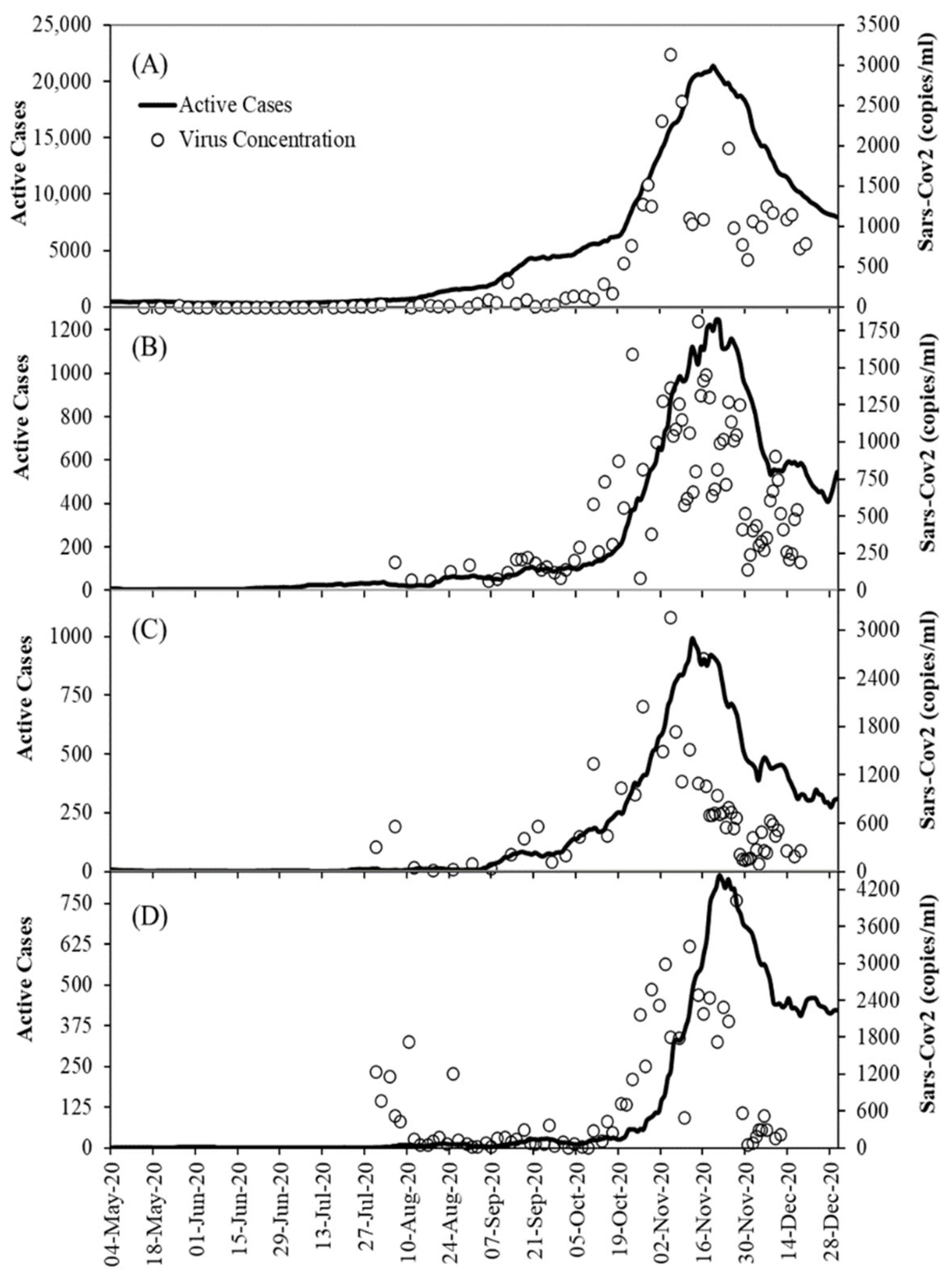
  • In the first category of the proposed modelling algorithm, the only source of information is the timeline of the wastewater signal, that is, the SARS-CoV-2 N1-gene copy numbers. Typically, this signal comes with significant noise and outliers, which influence the model training performance [45] Thus, a time series filtering method (the Spline method is used herein; [46]) is applied to filter out the noisy information adhered to the gene copy numbers.
  • In the second category, in addition to the gene copy number, the information on the number of tests taken in the communities is used where available (in only two of the case studies). In addition, we apply further data pre-processing steps such as population-normalisation of the viral load, time lag, and time series filtering (as in the first category), the details of which are discussed in Section 2.3, Section 2.4 and Section 2.5.
For both categories, the regressors were standardised because statistical models are sensitive to the data scales and units [47].
Parametric statistical models must be provided with basic parameter information prior to training, for example, the number of neighbours in the K-nearest neighbour method (KNN). To tune these parameters, a range of feasible values was initiated for each method investigated. Next, for each (parameter) option, a k-fold cross validation [48] is performed to assess the model performance, where the regressors are shuffled and split into training/testing subsets. Given the selected statistical models with different structural architectures, the models are trained and tested for both calibration and validation horizons. The regressors are then re-shuffled and partitioned for k trials, and the models are recalibrated and evaluated for each trial. Based on the model performance for all trials (folds) of the test subset, the optimum parameter values are determined according to the performance indicators (PI), that is, the mean and variance of the root mean square error (RMSE) and the Pearson’s correlation coefficient (R2).
Given the calibrated parameter values, for example, the number of neurons for an ANN-MLP, a k-fold cross validation is conducted again to estimate the model performance metrics under different subsets of data to compare model performances.

2.2. Dataset

The data used in this study stem from two different sources, that is, health agency information and wastewater-based epidemiology measurements taken at four treatment plants across Austria. The information taken from health services includes the daily time series of the number of COVID tests (total and positive cases) as well as the number of deaths and recovered patients. The number of currently active cases (A) is computed by the sum of daily confirmed cases ( N c ), the sum of deaths ( N d ), and the sum of (infected and then) recovered patients ( N r ) over the whole data series as follows:
A = N c N d N r
While incidence is typically expressed as the sum of new infections over a period of 7 or 14 days and scaled to 100,000 inhabitants, we use in the following “active cases” (A) as proxy. The advantage is that parameter A accounts directly for the duration of the infection and not by arbitrary summation over 7 or 14 days. From the treatment plants, not only are SARS-CoV-2 signals available, so are the inflow data and NH4-N concentration, which are used as population markers. The WWTPs are anonymised by the letters A–D, with the mean of the data given in Table 1 and the timeline of the raw SARS-CoV-2 signal as well as the active cases depicted in Figure 2. Details of the measurement programs are given elsewhere [21,45] and not repeated herein. Note that the wastewater composition in these four case studies is in the range typically found in industrialised countries and will thus not influence the methodology.
Note that the information on health services (regarding the test regime and active infection cases) is regional and is thus not entirely accurate for the WWTP catchments in question. That is, whereas the information on the urban environment coincides with the drained catchment, which is less accurate for suburbs and scattered communities. For instance, the calculated active cases for WWTP ‘B’ (Table 1) belong to the urban sub-catchment of the plant coverage area but only approximately. Half of the total number of active cases were measured at WWTP ‘B’. However, assuming B t and b t , as the time series of the number of active cases corresponding to the WWTP network and its main community, respectively, it was found that there is a nearly perfect linear relationship between B t and b t with a constant multiplier B t = k b t . For the WWTPs, ‘A’, ‘C’, and ‘D’, the multiplier was calculated as 1 k < 1.2 , and for ‘B’, we derive k = 2 . Given the linear relation, we must obtain a similar performance of the regression models for using a subset of the health information data instead of the accurate information.

2.3. Normalisation

Wastewater epidemiology assumes that each infected person sheds a certain amount of virus into the sewer network. For the normalisation of the SARS-Cov-2 signal, we compute the (theoretical) daily virus load per person based on the virus measurements in the WWTP by neglecting virus loss in transport and sampling:
L v i r u s = c v i r u s Q t P t
where L v i r u s is the daily virus load per person [genomes/cap/d], c v i r u s is the measured virus concentration at WWTP [genomes/m3/d], Q is the inflow to the WWTP [m3/d], and P is the population connected to the treatment plant. To estimate the dynamics of the population in the catchment, population-based biomarkers are suggested [43,44]. To capture the temporal dynamics, we assume that the population can be estimated by means of the daily personal biomarker load f b m [M/m3/d/cap] as follows:
P t = c b m Q t f b m
where c b m is the biomarker concentration (M/m3). Substituting Equation (3) into Equation (2) gives
L v i r u s = f b m   c v i r u s c b m
The use of an appropriate biomarker is the subject of many studies [49]; however, in this study, NH4-N was routinely monitored. To estimate the representative value f N H 4 N , the 50th percentile of the daily personal NH4-N load was determined during the period of the first lockdown in Austria (16 February to 13 April 2020) because the inflow fluctuations to the WWTPs are minimal during that period (see also [45]). fNH4N was found to range between 6.5 and 10.7 g NH4_N/m3/cap/d.

2.4. Filtering

The time series of both raw and normalised surveillance data comes with stochastic noise, resulting in misleading outputs caused by an overfitting to noisy data. In this study, the Spline algorithm was used to filter both the raw and normalised SARS-CoV-2 signals. The applicability and details of the Spline technique are widely discussed [50,51] and are also suggested by [45] specifically for WBE. The parameters for Spline smoothing are determined by calibration, using performance indicators such as mean absolute error, variability and Akaike information criterion [45].

2.5. Lagging

There is a temporal mismatch between the virus load measured at WWTP and the virological information released from clinical studies [21] which lags behind the wastewater signal. To adjust the time difference between the measured signals at the WWTPs and confirmed (active) cases, a cross-correlation analysis (CCA) was conducted to determine the best lagged explanatory variables. CCA is applied to a range of lagged time-series to determine significantly correlated signals with a at the level of 95% confidence. The CC significance limit is calculated as below [52]:
l = ± 1.96 n
where n is the number of observations. With the derived candidate lags (approximately 2–10 days) from the CCA, a linear model (LM) and ANOVA was set up for all possible combinations of lagged variables and the number of clinical tests where available. Finally, among the statistically meaningful model structures, we selected those with the lowest Akaike information criterion [53].

2.6. Regression Models

In this study, eight regression models that are popular in science and engineering prediction problems were evaluated and compared to predict their capability. The structure of the models in other studies and their application to COVID-19 modelling are presented in Table 2.

2.7. Evaluation

Under data limitations, a cross-validation procedure is applied to evaluate the performance of the regression models [67]. With this method, data are randomly shuffled and divided into training/testing subsets for model calibration and assessment. This is iterated k-times (k-fold) to ensure that the sampling process is unbiased. Herein, we apply a nine-fold cross-validation scheme to assess each implemented model. The results of a k-fold cross-validation are summarised with the mean and variance of the squared Pearson’s correlation coefficient (R2) and root mean square error (RMSE). The equations for R2 and RMSE are presented in the Appendix A.

3. Results and discussion

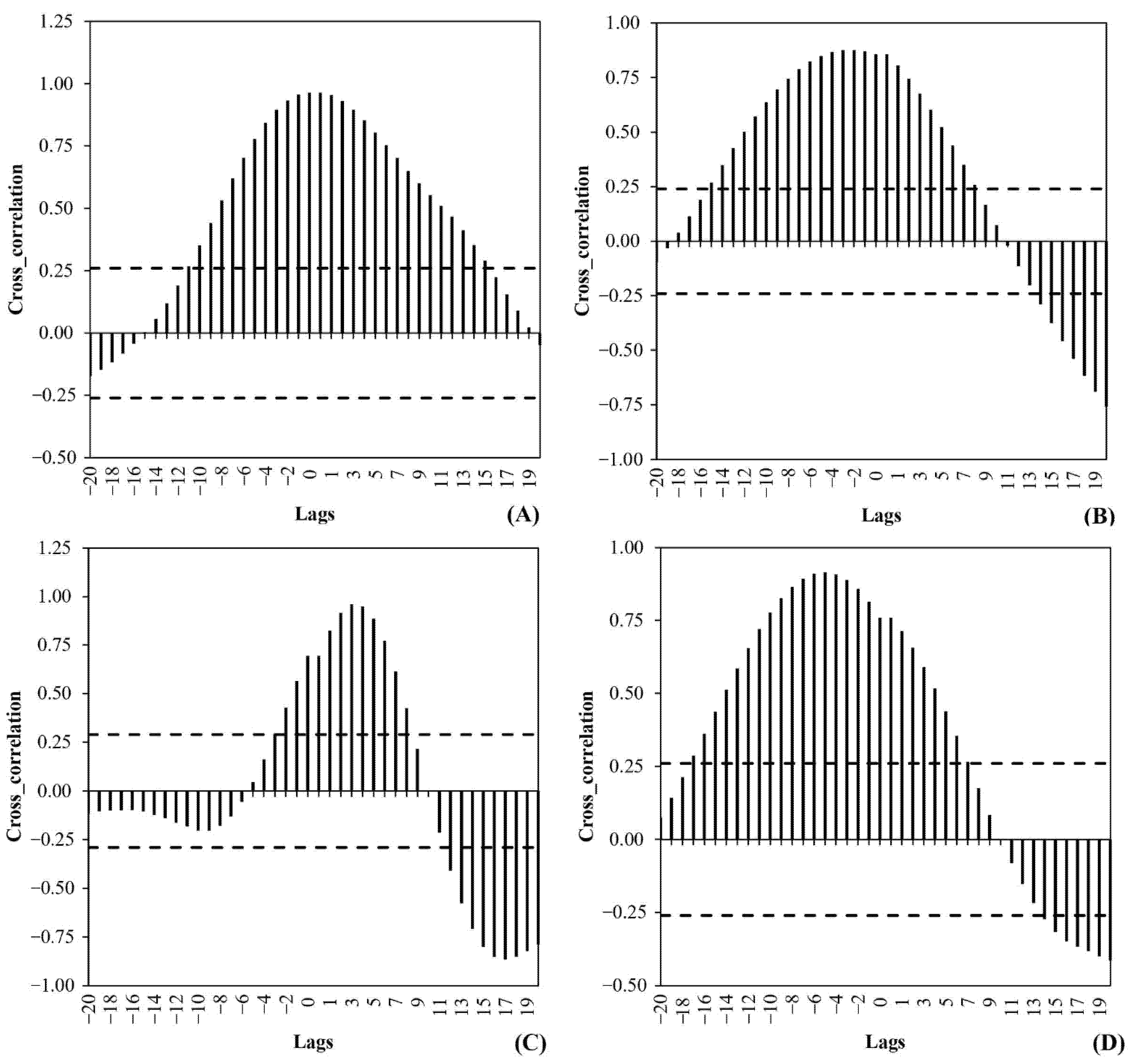
3.1. Time Series Lag

To identify the existing time lags between the viral load and the clinical information (see Section 2.5), the cross-correlation shown in Figure 3. Using Equation (5), CC significance limits are calculated, varying from ±0.25 to ±0.04.
For instance, in WWTP A, there is a significant correlation of between −11 and +15 days, whereas in WWTP B, it is approximately −15 to +8 days. Similarly, in WWTP D, a range of −16 to +7 days is computed as significant time shifts, whereas WWTP C has a significant time shift of −3 to +8 days. In general, in WWTPs A, B, and D, the corresponding CC plots show a similar time shift of (−14 ± 3) to (+10 ± 5), indicating WWTP C with different time-series characteristics.
In compliance with the objective of this study, which is the establishment of predictive regression models for active cases based on WWTP data, the forward correlation lags are neglected and model regressors are populated based on active backward-lagging time-series cases. To this end, assuming a bivariate model input, the combinations of active time-series cases with different lags were considered and analysed using an analysis of variance (ANOVA). For each treatment plant and under a confidence of 95%, the best time-series lags were selected using AIC [53]. In addition to the viral load, the number of tested persons available in the catchment of two WWTPs, A and B, is also considered as an ANOVA input.
Table 3 presents the results of the best linear model structures derived using AIC. Based on the table, the adjusted R2 values for WWTPs A and B are approximately 8% higher than those for WWTPs C and D, denoting the importance of the additional exogenous variable (number of tests), information that is missing for WWTPs C and D. Under a 95% confidence level, the model parameters (with the exception of the model A intercept) contribute significantly to the explanation of their respective variance in active cases. According to the results, SARS-CoV-2 signals with lags of (2, 4), (2, 7), (5, 7), and (3, 7) were found to be optimum regressors for the investigated cases.
The heat map shown in Figure 4 allows the identification of the significant values of the Pearson correlation coefficient [68] for different input signals: univariate (category 1) and multivariate (category 2) models.

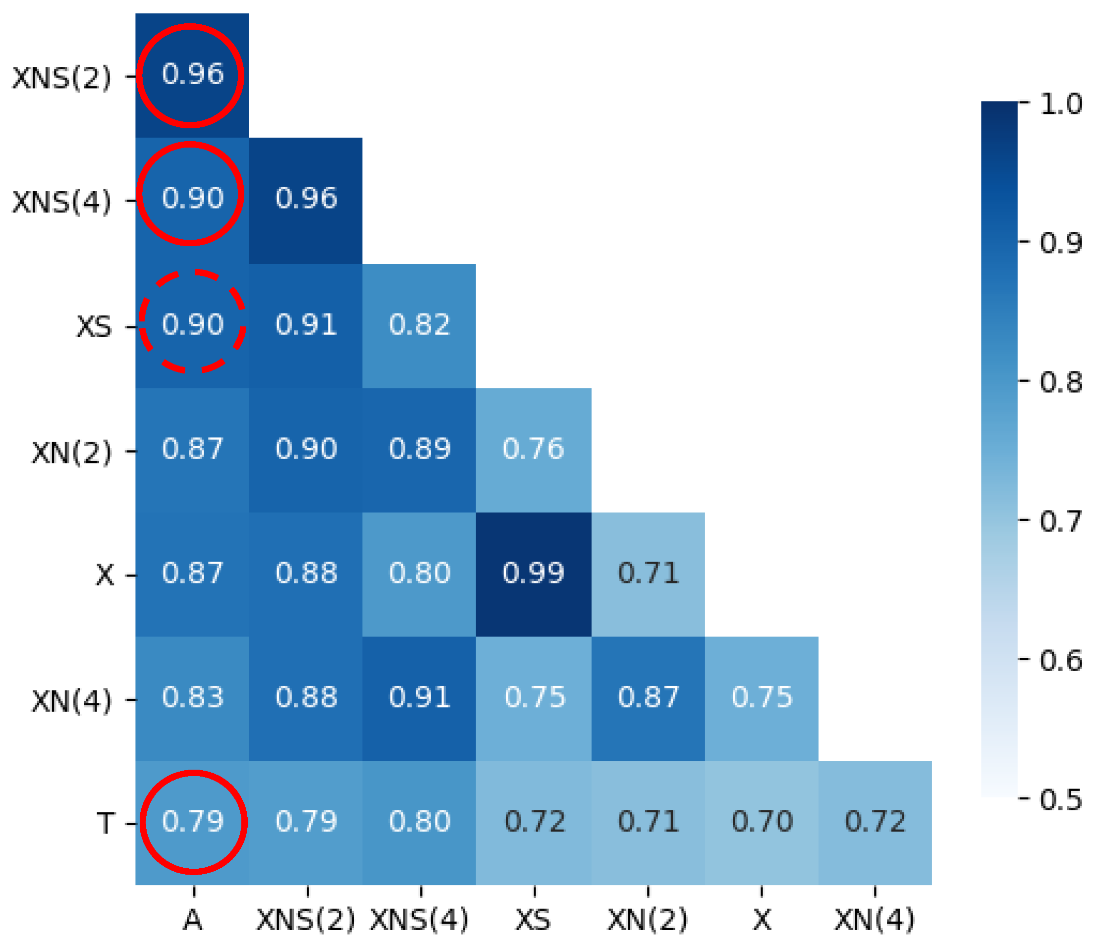
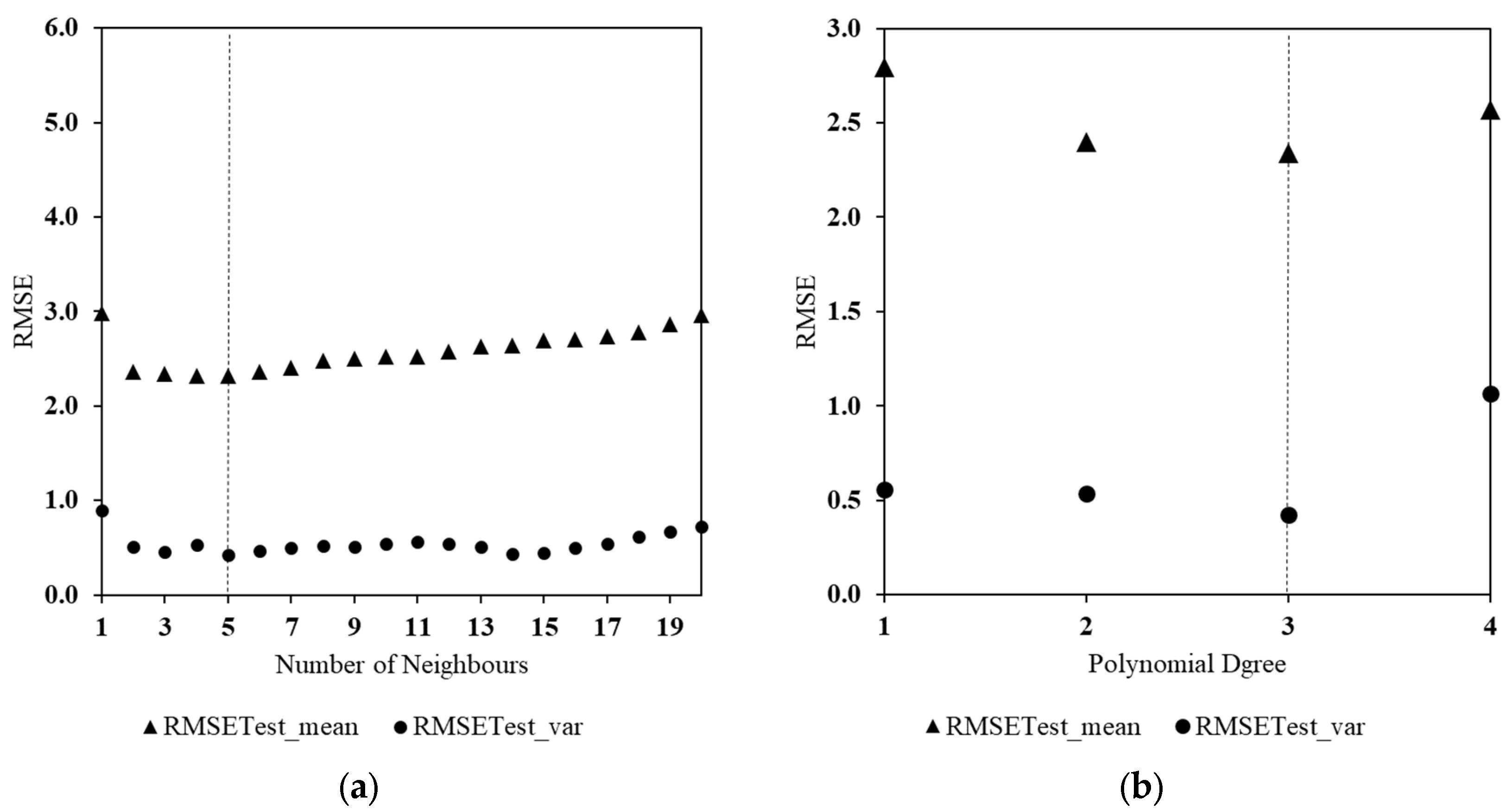
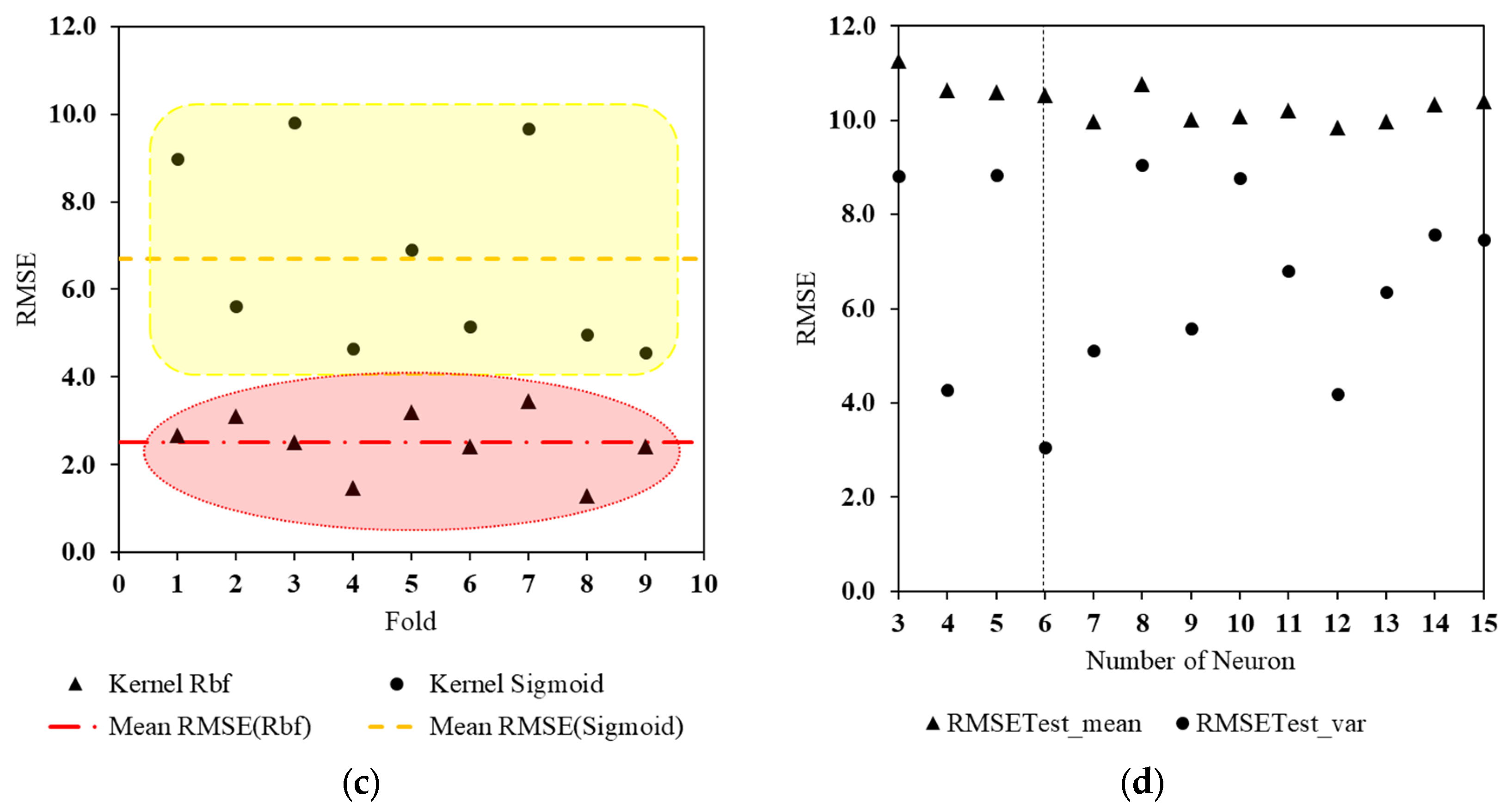
3.2. Global Parameter Tuning
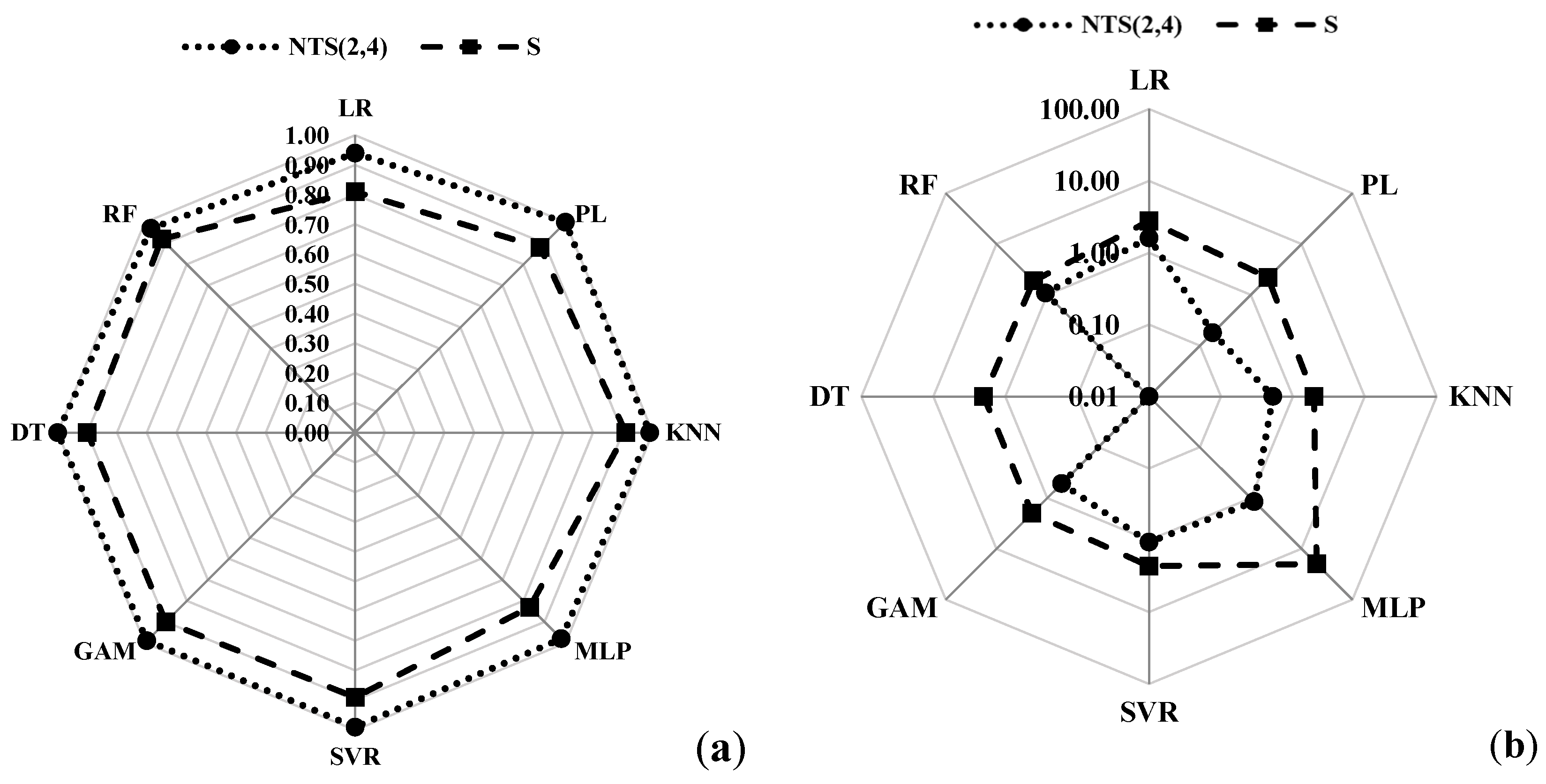
Given that most of the selected statistical models are parametric, a grid search is conducted to find the basic setup values that are optimum for those parameters (e.g., number of neurons). Accordingly, a multitude of regression models for different parameter ranges were evaluated. The models were calibrated and evaluated for the test subsets based on the mean and variance of the RMSE performance indicator. Figure 5 shows the resulting metrics of nine-fold randomly selected test subsets against the calibrated setup parameters of the models (e.g., KNN, MLP, SVR, polynomial, decision tree, and random forest) applied to the WWTP A data:
For example, as indicated in Figure 5, the order of the polynomial method and the depth of the random forest are calculated as 3 and 2, respectively. The same process was applied to all models at all WWTPs to ensure the model optimality.
Regarding the actual values of the parameters a comparison (and analysis of variation) is not meaningful as the values differ widely—especially for complex models. Only for linear models could a more rigorous comparison be conducted, but also here the variations are heavily influenced by the time lag. To conclude, it is not possible to derive a unique set of parameter values that result in a fair overall regression, but tuning is necessary for each site.

3.3. Model Metrics

Evaluating the regression models for the two input data categories (as described in Section 2.1), the R2 and RMSE metrics calculated for the different statistical models are plotted in Appendix B Figure A1 for the example of WWTP A. It is worth mentioning that the PI values for each station are based on the average of the metrics over a nine-fold trial. Models containing additional information (category 2) outweigh models that are fed only with a filtered SARS-CoV-2 signal (S), proving the importance of signal lagging, normalisation (N), and the number of tests taken (T) within the target communities. An increase in the model performance of approximately 10% to 20% and 1.0% to 5.0% in terms of R2 and RMSE, respectively, is observed (data found in Supplementary Materials Figures S1–S3).
Although the improvement varies for the different regression models, it can be deduced that all models perform better with additional information. In Figure 6, the model predictions regarding active cases are plotted for all implemented regression models in both univariate and multivariate approaches for the testing/training subsets for WWTP A. As shown in the figure, all models depict a superior fitness under the multivariate approach, particularly in terms of bias. An evaluation of the models for the test subset indicates a significant underestimation in the univariate models, whereas when applying additional information and conducting a multivariate analysis, a smaller bias is observed. Despite the improvement in the model metrics with multivariate data inputs, LR achieves the worst performance in both the training and test subsets. Because models such as RF, DT, and MLP tend to overfit in terms of calibration, they propagate larger biases during testing. Conversely, models such as KNN, PL, SVR, and GAM achieve an outstanding performance for both the testing and training subsets because they prevent an overfitting during the calibration. The results for the other three WWTPs are included in the Supplementary Materials (Figures S4–S6), the patterns of which are similar.

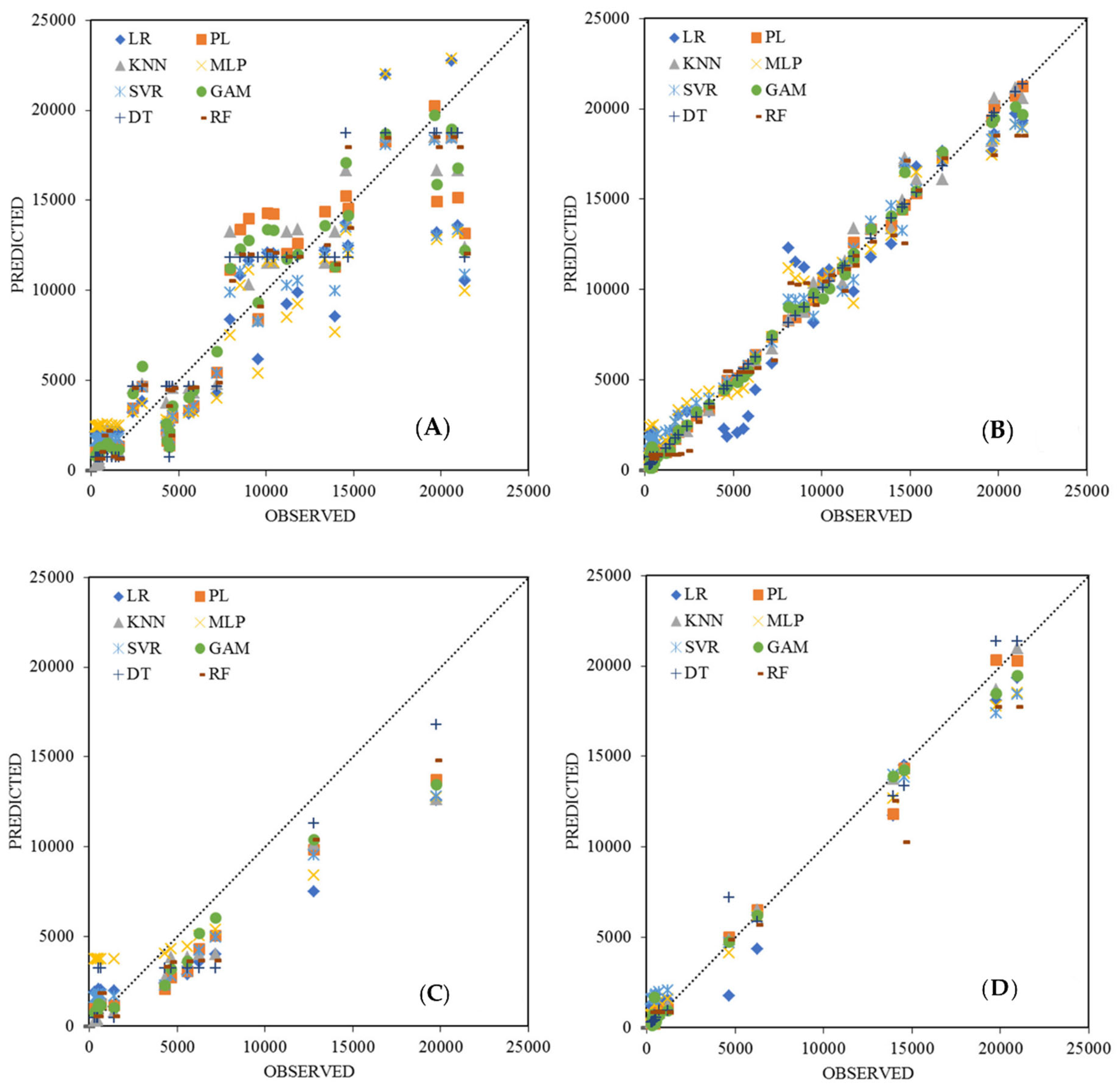
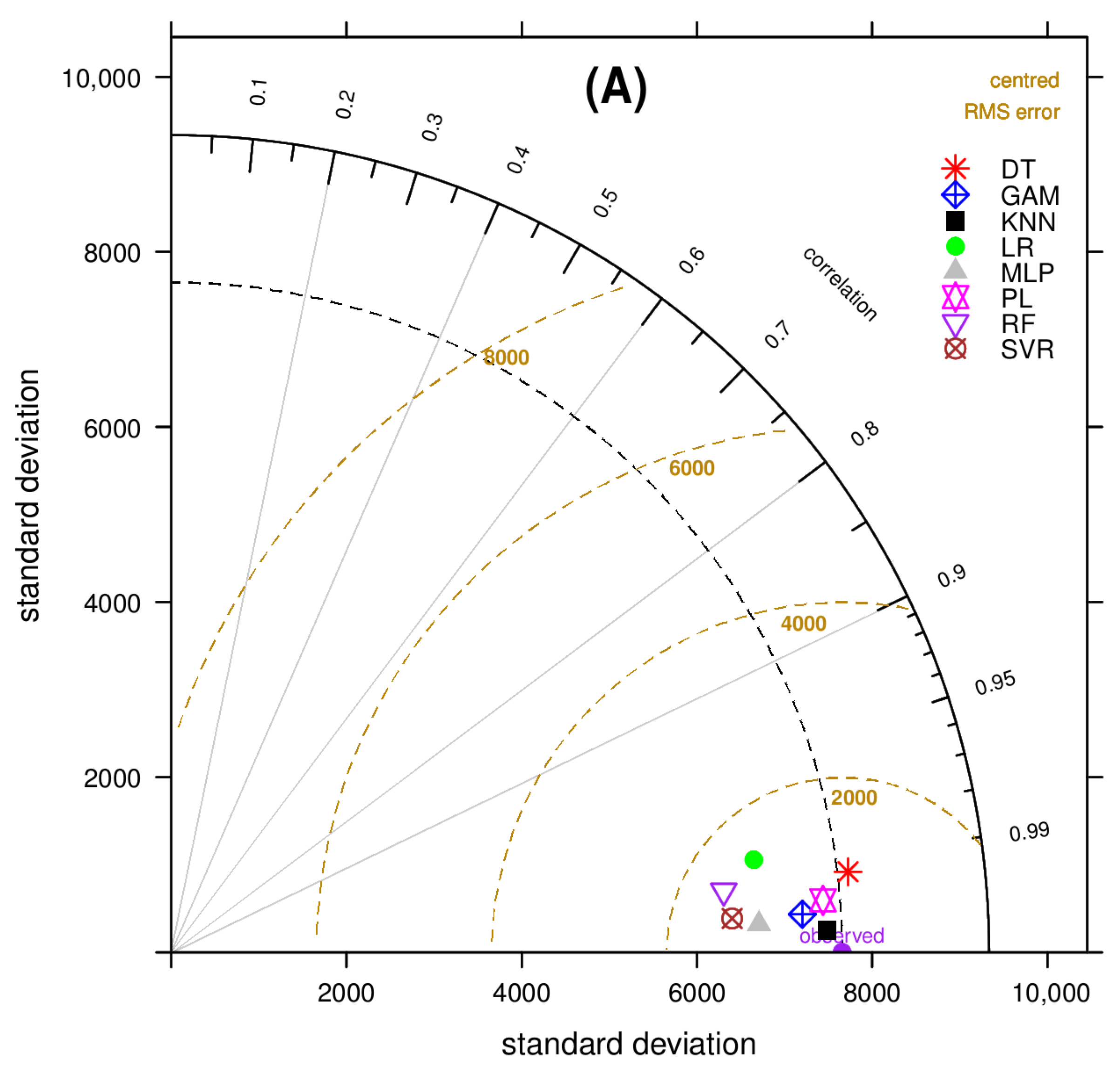
3.4. Model Comparison

To measure the degree of correspondence between the observed values and the predictions by the implemented models, a Taylor diagram (TD) [69] was drawn for the multivariate models under the test horizon (Figure 7). The closer the plotted model to the x-axis (indicating the observations), the lower the relative RMSE and the higher the correlation. The WWTP A, KNN, GAM, and PL models are closer to the point marked ‘observed’ data, with KNN appearing to be optimal. The TDs for the other three WWTPs are presented in the Supplementary Materials (Figure S7).
The TD of WWTP B indicates that the KNN, GAM, and PL models achieve a higher prediction accuracy, and KNN was again found to be the best option. For WWTPs C and D, the three best-simulated models are MLP, PL, and SVR, and SVR, KNN, and PL, respectively, where MLP and SVR are selected as the best regression models. In summary, Table 4 makes the following key conclusions from the Taylor diagram analysis: (i) the PL model is found most frequently to be among the top three options across all studied WWTPs, with a slight difference from the best model; (ii) the KNN model is the best model in the two larger communities (WWTPs A and B), followed by GAM; (iii) in the smaller communities, namely C and D, the SVR model tends to be more accurate, and was found to be the best and second best in WWTPs D and C, respectively, and iv) all models operate satisfactorily on a general level, even the multivariate LR model.
Based on the description in Section 3.3, and owing to the comparatively poor performance of the univariate models, only the results of the top-rated multivariate models categorised in Table 4 are shown in Figure 8. As can be seen, there is a better fit between the predicted values and the observed time series at WWTPs A and B, which is attributed to the availability of the number of tests taken in these case studies. Note that the timeline of the SARS-CoV-2 data in Figure 8 is the smoothed and normalized signal only, but without the influence of lagging—as taken into account in the modelling.

4. Conclusions

In the present study, we systematically investigated the correlation of the SARS-CoV-2 gene copy number found by WBE and the incidence values derived from individual testing. The study compared eight different regression models for a dataset monitored for four WWTPs in Austria. The key findings are as follows:
  • There is a consistent time shift between the (earlier) wastewater signal and the clinical test records, varying from 2 to 7 days in our dataset—depending both on time period and site;
  • A thorough pre-processing of the data, such as population-based normalisation and smoothing, leads to more robust models and is important for practical application;
  • The inclusion of additional information (most importantly the time lag and number of tests taken) by applying multivariate models significantly increases the performance of all investigated models;
  • All multivariate models are generally applicable for the regression, and even a simple linear regression can be used, despite showing the poorest performance.
  • While the differences are small, PL and KNN outperform more complex models such as GAM, SVR, and MLP;
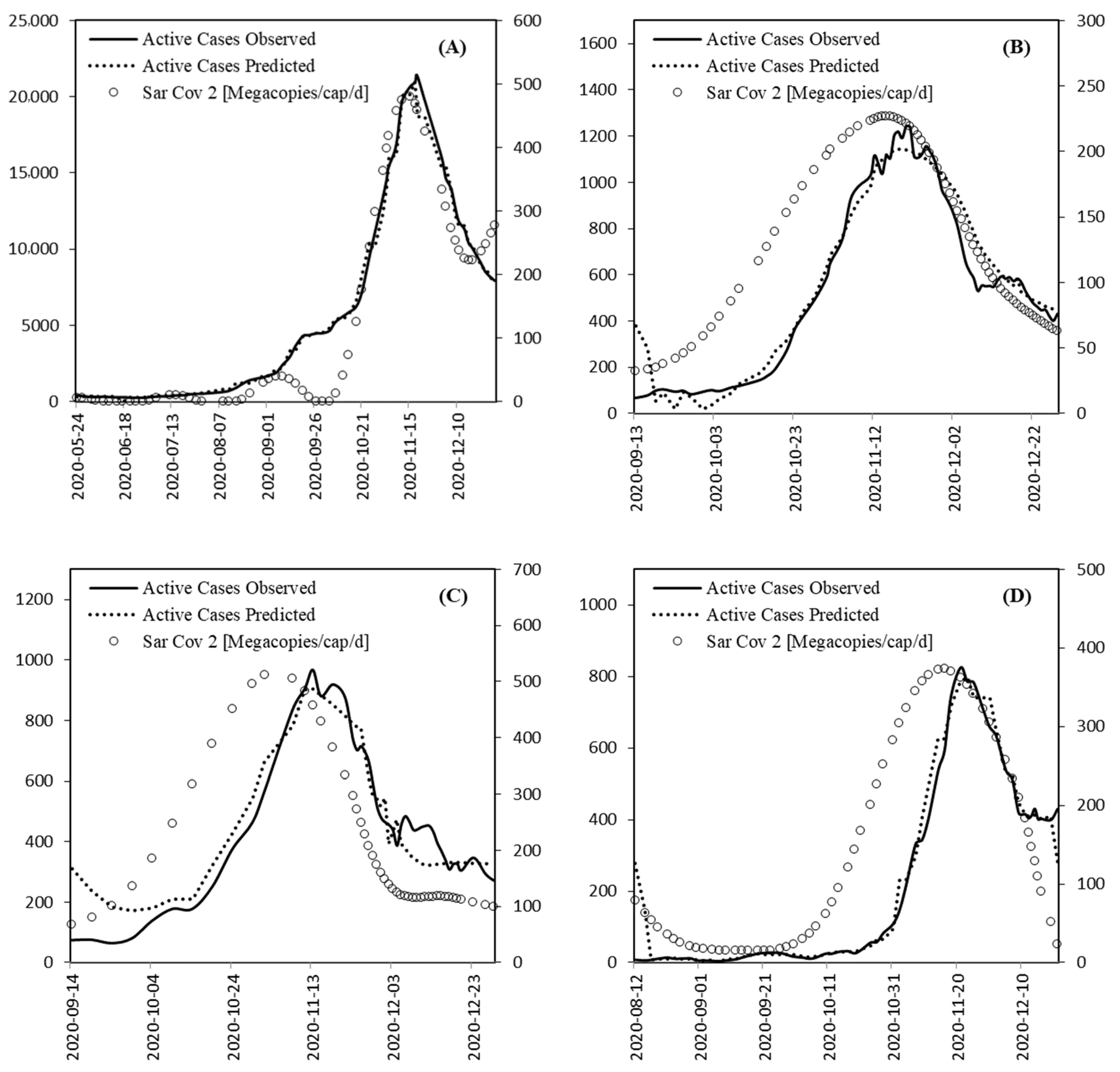
  • As seen from above, regression between the wastewater signal and incidence values is derived easily—also, in a practical context. The information supplements—but could even replace—individual testing for incidence.

Supplementary Materials

The following are available online at https://www.mdpi.com/article/10.3390/ijerph182010778/s1, Figure S1: Model performance as spider chart—WWTP B. Left: RMSE and right: RSQ metric comparing signal (S) only with combined information of signal (S), normalisation (N) and tests taken (T). Figure S2: Model performance as spider chart—WWTP C. Left: RMSE and right: RSQ metric comparing signal (S) only with combined information of signal (S), normalisation (N) and tests taken (T). Figure S3: Model performance as spider chart—WWTP D. Left: RMSE and right: RSQ metric comparing signal (S) only with combined information of signal (S), normalisation (N) and tests taken (T). Figure S4: Visualisation of the number of active cases recorded versus model prediction in WWTP B: (i) and (ii) model predictions against recorded data for training subset under univariate and multivariate inputs, respectively, and (iii) and (iv) the same plots for the testing subset. Figure S5: Visualisation of the number of active cases recorded versus model prediction in WWTP C: (i) and (ii) model predictions against recorded data for training subset under univariate and multivariate inputs, respectively, and (iii) and (iv) the same plots for the testing subset. Figure S6: Visualisation of the number of active cases recorded versus model prediction in WWTP D: (i) and (ii) model predictions against recorded data for training subset under univariate and multivariate inputs, respectively, and (iii) and (iv) the same plots for the testing subset. Figure S7: Taylor diagram, displaying statistical comparison of the eight model predictions against the actual number of recorded active cases—WWTP B, C and D.

Author Contributions

Conceptualization, P.A., R.A. and W.R.; methodology, P.A. and R.A.; software, P.A. and R.A.; validation R.M. and M.M.; investigation, R.M. and N.K.; data curation, M.M.; writing—original draft preparation, P.A.; writing—review and editing, W.R., H.I. and R.M.; supervision, W.R.; project administration, W.R. and H.I.; funding acquisition, W.R. and H.I. All authors have read and agreed to the published version of the manuscript.

Funding

This study was funded by the Austrian Federal Ministry of Education, Science and Research, the Austrian Federal Ministry of Agriculture, Regions and Tourism, the City of Vienna, the Federal States of Carinthia, Salzburg, and Vorarlberg as well as the Austrian Association of Cities and Towns. The APC was funded by University Innsbruck.

Institutional Review Board Statement

Not applicable.

Informed Consent Statement

Not applicable.

Data Availability Statement

Publicly available data used in this study can be found at https://covid19-dashboard.ages.at (accessed on 10 February 2021).

Acknowledgments

We would like to thank the staff of the treatment plants involved for their support and the use of the wastewater titer measurement data.

Conflicts of Interest

The authors declare no conflict of interest. The funders had no role in the design of the study; in the collection, analyses, or interpretation of data; in the writing of the manuscript, or in the decision to publish the results.

Appendix A

The equation of the coefficient of determination is:
R 2 = SS res SS tot
where {\displaystyle R^{2}=1-{SS_{\rm {res}}\over SS_{\rm {tot}}}\,} S S r e s refers to the residual sum of squares and S S t o t is the total sum of squares. In the ideal condition of any model, when both observation and simulated dataset are perfectly fitted, the result of R2 is 1.
To measure errors as a result of model prediction/fitness the RMSE is calculated as:
RMSE = i = 1 N ( X i X ^ i ) 2 N
where X i is the measured output, X ^ i is the model fitness/prediction output, and N is the number of observations. The lower RMSE, the better the fitness; becoming zero when the model fitness/prediction is perfectly matching the observation records.

Appendix B

Figure A1. Model performance as spider chart—WWTP A. (a) RMSE, and (b) RSQ metric comparing signal (S) only with combined information of signal (S), normalisation (N) and tests taken (T).
Ijerph 18 10778 g0a1

References

  1. Metcalf, T.G.; Melnick, J.L.; Estes, M.K. Environmental Virology: From Detection of Virus in Sewage and Water by Isolation to Identification by Molecular Biology—A Trip of over 50 Years. Annu. Rev. Microbiol. 1995, 49, 461–487. [Google Scholar] [CrossRef] [PubMed]
  2. Kittigul, L.; Raengsakulrach, B.; Siritantikorn, S.; Kanyok, R.; Utrarachkij, F.; Diraphat, P.; Thirawuth, V.; Siripanichgon, K.; Pungchitton, S.; Chitpirom, K.; et al. Detection of Poliovirus, Hepatitis A Virus and Rotavirus from Sewage and Water Samples. Southeast Asian J. Trop. Med. Public Health 2000, 31, 41–46. [Google Scholar] [PubMed]
  3. Medema, G.; Heijnen, L.; Elsinga, G.; Italiaander, R.; Brouwer, A. Presence of SARS-Coronavirus-2 RNA in Sewage and Correlation with Reported COVID-19 Prevalence in the Early Stage of the Epidemic in the Netherlands. Environ. Sci. Technol. Lett. 2020, 7, 511–516. [Google Scholar] [CrossRef]
  4. Heijnen, L.; Medema, G. Surveillance of Influenza A and the Pandemic Influenza A (H1N1) 2009 in Sewage and Surface Water in the Netherlands. J. Water Health 2011, 9, 434–442. [Google Scholar] [CrossRef] [Green Version]
  5. Prado, T.; Fumian, T.M.; Mannarino, C.F.; Resende, P.C.; Motta, F.C.; Eppinghaus, A.L.F.; Chagas do Vale, V.H.; Braz, R.M.S.; de Andrade, J.D.S.R.; Maranhão, A.G.; et al. Wastewater-Based Epidemiology as a Useful Tool to Track SARS-CoV-2 and Support Public Health Policies at Municipal Level in Brazil. Water Res. 2021, 191, 116810. [Google Scholar] [CrossRef]
  6. Sims, N.; Kasprzyk-Hordern, B. Future Perspectives of Wastewater-Based Epidemiology: Monitoring Infectious Disease Spread and Resistance to the Community Level. Environ. Int. 2020, 139, 105689. [Google Scholar] [CrossRef]
  7. Ahmed, W.; Angel, N.; Edson, J.; Bibby, K.; Bivins, A.; O’Brien, J.W.; Mueller, J.F. First confirmed detection of SARS-CoV-2 in untreated wastewater in Australia: A proof of concept for the wastewater surveillance of COVID-19 in the community. Sci. Total Environ. 2020, 728, 138764. [Google Scholar] [CrossRef]
  8. Mallapaty, S. How Sewage Could Reveal True Scale of Coronavirus Outbreak. Nature 2020, 580, 176–177. [Google Scholar] [CrossRef] [Green Version]
  9. Mlejnkova, H.; Sovova, K.; Vasickova, P.; Ocenaskova, V.; Jasikova, L.; Juranova, E. Preliminary Study of SARS-CoV-2 Occurrence in Wastewater in the Czech Republic. Int. J. Environ. Res. Public Health 2020, 17, 5508. [Google Scholar] [CrossRef]
  10. Zhang, D.; Wang, X.; Gao, L.; Gong, Y. Predict and Analyze Exchange Rate Fluctuations Accordingly Based on Quantile Regression Model and K-Nearest Neighbor. J. Phys. Conf. Ser. 2021, 1813, 012016. [Google Scholar] [CrossRef]
  11. Arora, S.; Nag, A.; Sethi, J.; Rajvanshi, J.; Saxena, S.; Shrivastava, S.K.; Gupta, A.B. Sewage surveillance for the presence of SARS-CoV-2 genome as a useful wastewater based epidemiology (WBE) tracking tool in India. Water Sci. Technol. 2020, 82, 2823–2836. [Google Scholar] [CrossRef]
  12. Murakami, M.; Hata, A.; Honda, R.; Watanabe, T. Letter to the Editor: Wastewater-Based Epidemiology Can Overcome Representativeness and Stigma Issues Related to COVID-19. Environ. Sci. Technol. 2020, 54, 5311. [Google Scholar] [CrossRef] [PubMed] [Green Version]
  13. Xagoraraki, I.; O’Brien, E. Wastewater-Based Epidemiology for Early Detection of Viral Outbreaks. In Women in Engineering and Science; Springer: Cham, Switzerland, 2020; pp. 75–97. [Google Scholar] [CrossRef] [Green Version]
  14. Gonzalez, R.; Curtis, K.; Bivins, A.; Bibby, K.; Weir, M.H.; Yetka, K.; Thompson, H.; Keeling, D.; Mitchell, J.; Gonzalez, D. COVID-19 Surveillance in Southeastern Virginia Using Wastewater-Based Epidemiology. Water Res. 2020, 186, 116296. [Google Scholar] [CrossRef] [PubMed]
  15. Breiman, L. Random Forests. Mach. Learn. 2001, 45, 5–32. [Google Scholar] [CrossRef] [Green Version]
  16. Wurtzer, S.; Marechal, V.; Mouchel, J.M.; Maday, Y.; Teyssou, R.; Richard, E.; Almayrac, J.L.; Moulin, L. Evaluation of Lockdown Impact on SARS-CoV-2 Dynamics Through Viral Genome Quantification in Paris Wastewaters. medRxiv 2020. [Google Scholar] [CrossRef]
  17. Kumar, M.; Patel, A.K.; Shah, A.V.; Raval, J.; Rajpara, N.; Joshi, M.; Joshi, C.G. First Proof of the Capability of Wastewater Surveillance for COVID-19 in India through Detection of Genetic Material of SARS-CoV-2. Sci. Total Environ. 2020, 746, 141326. [Google Scholar] [CrossRef]
  18. Wu, F.; Zhang, J.; Xiao, A.; Gu, X.; Lee, W.L.; Armas, F.; Kauffman, K.; Hanage, W.; Matus, M.; Ghaeli, N.; et al. SARS-CoV-2 Titers in Wastewater Are Higher than Expected from Clinically Confirmed Cases. mSystems 2020, 5, e00614-20. [Google Scholar] [CrossRef] [PubMed]
  19. D’Aoust, P.M.; Graber, T.E.; Mercier, E.; Montpetit, D.; Alexandrov, I.; Neault, N.; Baig, A.T.; Mayne, J.; Zhang, X.; Alain, T.; et al. Catching a Resurgence: Increase in SARS-CoV-2 Viral RNA Identified in Wastewater 48 h before COVID-19 Clinical Tests and 96 h before Hospitalizations. Sci. Total Environ. 2021, 770, 145319. [Google Scholar] [CrossRef] [PubMed]
  20. Randazzo, W.; Truchado, P.; Cuevas-Ferrando, E.; Simón, P.; Allende, A.; Sánchez, G. SARS-CoV-2 RNA in Wastewater Anticipated COVID-19 Occurrence in a Low Prevalence Area. Water Res. 2020, 181, 115942. [Google Scholar] [CrossRef]
  21. Markt, R.; Bergthaler, A.; Bock, C.; Büchel-Marxer, M.; Grünbacher, D.; Mayr, M.; Peer, E.; Pedrazzini, M.; Penz, T.; Rauch, W.; et al. First detection and abundance of SARS-CoV-2 in wastewater in Liechtenstein: A surveillance in estimation of prevalence and impact of the SARS-CoV-2 B. 1.1.7 variant. 2021, submitted. [Google Scholar]
  22. Breslow, N.E. Generalized Linear Models: Checking Assumptions and Strengthening Conclusions. Stat. Appl. 1996, 8, 23–41. [Google Scholar]
  23. Osborne, J.W.; Waters, E. Four Assumptions of Multiple Regression That Researchers Should Always Test. Pract. Assess. Res. Eval. 2002, 8, 2. [Google Scholar]
  24. Centers for Disease Control and Prevention. Evaluating and Testing Persons for Coronavirus Disease 2019 (COVID-19); Centers for Disease Control and Prevention: Atlanta, GA, USA, 2020. [Google Scholar]
  25. Pettit, S.D.; Jerome, K.R.; Rouquié, D.; Mari, B.; Barbry, P.; Kanda, Y.; Matsumoto, M.; Hester, S.; Wehmas, L.; Botten, J.W.; et al. “All In”: A Pragmatic Framework for COVID-19 Testing and Action on a Global Scale. EMBO Mol. Med. 2020, 12, e12634. [Google Scholar] [CrossRef]
  26. Rashid, Z.Z.; Othman, S.N.; Abdul Samat, M.N.; Ali, U.K.; Wong, K.K. Diagnostic Performance of COVID-19 Serology Assays. Malays. J. Pathol. 2020, 42, 13–21. [Google Scholar]
  27. Gudbjartsson, D.F.; Helgason, A.; Jonsson, H.; Magnusson, O.T.; Melsted, P.; Norddahl, G.L.; Saemundsdottir, J.; Sigurdsson, A.; Sulem, P.; Agustsdottir, A.B.; et al. Spread of SARS-CoV-2 in the Icelandic Population. N. Engl. J. Med. 2020, 382, 2302–2315. [Google Scholar] [CrossRef] [PubMed]
  28. Chen, Y.; Chen, L.; Deng, Q.; Zhang, G.; Wu, K.; Ni, L.; Yang, Y.; Liu, B.; Wang, W.; Wei, C.; et al. The Presence of SARS-CoV-2 RNA in the Feces of COVID-19 Patients. J. Med. Virol. 2020, 92, 833–840. [Google Scholar] [CrossRef] [PubMed] [Green Version]
  29. Yang, R.; Gui, X.; Xiong, Y. Comparison of Clinical Characteristics of Patients with Asymptomatic vs. Symptomatic Coronavirus Disease 2019 in Wuhan, China. JAMA Netw. Open 2020, 3, e2010182. [Google Scholar] [CrossRef]
  30. Bi, Q.; Wu, Y.; Mei, S.; Ye, C.; Zou, X.; Zhang, Z.; Liu, X.; Wei, L.; Truelove, S.A.; Zhang, T.; et al. Epidemiology and transmission of COVID-19 in 391 cases and 1286 of their close contacts in Shenzhen, China: A retrospective cohort study. Lancet Infect Dis. 2020, 20, 911–919. [Google Scholar] [CrossRef]
  31. Tang, A.N.; Tong, Z.D.; Wang, H.L.; Dai, Y.X.; Li, K.F.; Liu, J.N.; Wu, W.J.; Yuan, C.; Yu, M.L.; Li, P.; et al. Detection of Novel Coronavirus by RT-PCR in Stool Specimen from Asymptomatic Child, China. Emerg. Infect. Dis. 2020, 26, 1337–1339. [Google Scholar] [CrossRef]
  32. Banks, A.P.; Lai, F.Y.; Mueller, J.F.; Jiang, G.; Carter, S.; Thai, P.K. Potential impact of the sewer system on the applicability of alcohol and tobacco biomarkers in wastewater-based epidemiology. Drug Test. Anal. 2020, 10, 530–538. [Google Scholar] [CrossRef] [PubMed]
  33. Eramo, A.; Morales Medina, W.R.M.; Fahrenfeld, N.L. Factors Associated with Elevated Levels of Antibiotic Resistance Genes in Sewer Sediments and Wastewater. Environ. Sci. Water Res. Technol. 2020, 6, 1697–1710. [Google Scholar] [CrossRef] [PubMed]
  34. Rath, S.; Tripathy, A.; Tripathy, A.R. Prediction of New Active Cases of Coronavirus Disease (COVID-19) Pandemic Using Multiple Linear Regression Model. Diabetes Metab. Syndr. 2020, 14, 1467–1474. [Google Scholar] [CrossRef] [PubMed]
  35. Muhammad, L.J.; Islam, M.M.; Usman, S.S.; Ayon, S.I. Predictive Data Mining Models for Novel Coronavirus (COVID-19) Infected Patients’ Recovery. SN Comput. Sci. 2020, 1, 206. [Google Scholar] [CrossRef] [PubMed]
  36. Sujath, R.; Chatterjee, J.M.; Hassanien, A.E. A Machine Learning Forecasting Model for COVID-19 Pandemic in India. Stoch. Environ. Res. Risk Assess. 2020, 34, 959–972. [Google Scholar] [CrossRef] [PubMed]
  37. Saqib, M. Forecasting COVID-19 Outbreak Progression Using Hybrid Polynomial-Bayesian Ridge Regression Model. Appl. Intell. 2021, 51, 2703–2713. [Google Scholar] [CrossRef]
  38. Parbat, D.; Chakraborty, M. A Python Based Support Vector Regression Model for Prediction of COVID19 Cases in India. Chaos Solitons Fract. 2020, 138, 109942. [Google Scholar] [CrossRef] [PubMed]
  39. Fayyoumi, E.; Idwan, S.; AboShindi, H. Machine Learning and Statistical Modelling for Prediction of Novel COVID-19 Patients Case Study: Jordan. IJACSA Int. J. Adv. Comput. Sci. Appl. 2020, 11, 122–126. [Google Scholar] [CrossRef]
  40. Vallejo, J.A.; Rumbo-Feal, S.; Conde-Pérez, K.; López-Oriona, Á.; Tarrío, J.; Reif, R.; Ladra, S.; Rodiño-Janeiro, B.K.; Nasser, M.; Cid, Á.; et al. Highly Predictive Regression Model of Active Cases of COVID-19 in a Population by Screening Wastewater Viral Load. medRxiv 2020. [Google Scholar] [CrossRef]
  41. Hemalatha, M.; Kiran, U.; Kuncha, S.K.; Kopperi, H.; Gokulan, C.G.; Mohan, S.V.; Mishra, R.K. Surveillance of SARS-CoV-2 Spread Using Wastewater-Based Epidemiology: Comprehensive Study. Sci. Total Environ. 2021, 768, 144704. [Google Scholar] [CrossRef]
  42. Huang, Y.; Zhang, Y.; Li, N.; Chambers, J. Robust Student’st Based Nonlinear Filter and Smoother. IEEE Trans. Aerosp. Electron. Syst. 2016, 52, 2586–2596. [Google Scholar] [CrossRef] [Green Version]
  43. Been, F.; Rossi, L.; Ort, C.; Rudaz, S.; Delémont, O.; Esseiva, P. Population normalization with ammonium in wastewater-based epidemiology: Application to illicit drug monitoring. Environ. Sci. Technol. 2014, 48, 8162–8169. [Google Scholar] [CrossRef] [PubMed]
  44. Tscharke, B.J.; O’Brien, J.W.; Ort, C.; Grant, S.; Gerber, C.; Bade, R.; Thai, P.K.; Thomas, K.V.; Mueller, J.F. Harnessing the Power of the Census: Characterizing Wastewater Treatment Plant Catchment Populations for Wastewater-Based Epidemiology. Environ. Sci. Technol. 2019, 53, 10303–10311. [Google Scholar] [CrossRef] [PubMed]
  45. Arabzadeh, R.; Gruenbacher, D.M.; Insam, H.; Kreuzinger, N.; Markt, R.; Rauch, W. Data filtering methods for SARS-CoV-2 wastewater surveillance. Water Sci. Technol. 2021, 84, 1324–1339. [Google Scholar] [CrossRef] [PubMed]
  46. Reinsch, C.H. Smoothing by Spline Functions. Numer. Math. 1967, 10, 177–183. [Google Scholar] [CrossRef]
  47. Sharma, P.; Singh, J. Machine Learning Based Effort Estimation Using Standardization. In Proceedings of the 2018 International Conference on Computing, Power and Communication Technologies (GUCON), Greater Noida, India, 28–29 September 2018; IEEE Publications: Piscataway, NJ, USA, 2019; pp. 716–720. [Google Scholar]
  48. Stone, M. An Asymptotic Equivalence of Choice of Model by Cross-Validation and Akaike’s Criterion. J. R. Stat. Soc. B 1977, 39, 44–47. [Google Scholar] [CrossRef]
  49. Choi, P.M.; Tscharke, B.J.; Donner, E.; O’Brien, J.W.; Grant, S.C.; Kaserzon, S.L.; Mackie, R.; O’Malley, E.; Crosbie, N.D.; Thomas, K.V.; et al. Wastewater-Based Epidemiology Biomarkers: Past, Present and Future. TrAC Trends Anal. Chem. 2018, 105, 453–469. [Google Scholar] [CrossRef]
  50. Eubank, R.L. Spline Smoothing and Nonparametric Regression; Marcel Dekker Inc.: New York, NY, USA, 1988. [Google Scholar]
  51. Silverman, B.W. Some Aspects of the Spline Smoothing Approach to Non-Parametric Regression Curve Fitting. J. R. Stat. Soc. B 1985, 47, 1–21. [Google Scholar] [CrossRef]
  52. Dean, R.T.; Dunsmuir, W.T. Dangers and Uses of Cross-Correlation in Analyzing Time Series in Perception, Performance, Movement, and Neuroscience: The Importance of Constructing Transfer Function Autoregressive Models. Behav. Res. Methods 2016, 48, 783–802. [Google Scholar] [CrossRef] [Green Version]
  53. Akaike, H. A new look at the statistical model identification. IEEE Trans. Automat. Contr. 1974, 19, 716–723. [Google Scholar] [CrossRef]
  54. Yan, X.; Su, X. Linear Regression Analysis: Theory and Computing; World Scientific Publishing: Singapore, 2009. [Google Scholar]
  55. Stigler, S.M. Gergonne’s 1815 Paper on the Design and Analysis of Polynomial Regression Experiments. Hist. Math. 1974, 1, 431–439. [Google Scholar] [CrossRef] [Green Version]
  56. Amar, L.A.; Taha, A.A.; Mohamed, M.Y. Prediction of the final size for COVID-19 epidemic using machine learning: A case study of Egypt. Infect. Dis. Model. 2020, 5, 622–634. [Google Scholar] [CrossRef]
  57. Zhang, S.; Li, X.; Zong, M.; Zhu, X.; Cheng, D. Learning k for kNN Classification. ACM Trans. Intell. Syst. Technol. 2017, 8, 1–19. [Google Scholar] [CrossRef] [Green Version]
  58. Pourhomayoun, M.; Shakibi, M. Predicting Mortality Risk in Patients with COVID-19 Using Artificial Intelligence to Help Medical Decision-Making. medRxiv 2020. [Google Scholar] [CrossRef] [Green Version]
  59. Hastie, T.; Tibshirani, R.; Friedman, J. The Elements of Statistical Learning: Data Mining, Inference, and Prediction; Springer: Berlin/Heidelberg, Germany, 2009. [Google Scholar]
  60. Awad, M.; Khanna, R. Support vector regression. In Efficient Learning Machines; Apress: Berkeley, CA, USA, 2015; pp. 67–80. [Google Scholar]
  61. Ribeiro, M.H.D.M.; da Silva, R.G.; Mariani, V.C.; Coelho, L.D.S. Short-Term Forecasting COVID-19 Cumulative Confirmed Cases: Perspectives for Brazil. Chaos Solitons Fract. 2020, 135, 109853. [Google Scholar] [CrossRef]
  62. Hastie, T.J.; Tibshirani, R.J. Generalized Additive Models. Stat. Sci. 1986, 1, 297–310. [Google Scholar] [CrossRef]
  63. Prata, D.N.; Rodrigues, W.; Bermejo, P.H. Temperature Significantly Changes COVID-19 Transmission in (Sub) Tropical Cities of Brazil. Sci. Total Environ. 2020, 729, 138862. [Google Scholar] [CrossRef] [PubMed]
  64. Loh, W.Y. Classification and Regression Trees. WIREs Data Min. Knowl. Discov. 2011, 1, 14–23. [Google Scholar] [CrossRef]
  65. Karnon, J. A Simple Decision Analysis of a Mandatory Lockdown Response to the COVID-19 Pandemic. Appl. Health Econ. Health Policy 2020, 18, 329–331. [Google Scholar] [CrossRef] [PubMed] [Green Version]
  66. Prakash, K.B.; Imambi, S.S.; Ismail, M.; Kumar, T.P.; Pawan, Y.N. Analysis, Prediction and Evaluation of COVID-19 Datasets Using Machine Learning Algorithms. Int. J. Emerg. Trends Eng. Res. 2020, 5, 2199–2204. [Google Scholar] [CrossRef]
  67. Picard, R.R.; Cook, R.D. Cross-Validation of Regression Models. J. Am. Stat. Assoc. 1984, 79, 575–583. [Google Scholar] [CrossRef]
  68. Benesty, J.; Chen, J.; Huang, Y.; Cohen, I. Pearson correlation coefficient. In Noise Reduction in Speech Processing; Springer: Berlin/Heidelberg, Germany, 2009; pp. 1–4. [Google Scholar] [CrossRef]
  69. Taylor, K.E. Summarizing Multiple Aspects of Model Performance in a Single Diagram. J. Geophys. Res. 2001, 106, 7183–7192. [Google Scholar] [CrossRef]
Figure 1. Modelling workflow.
Ijerph 18 10778 g001
Figure 2. Raw data timeline of SARS-CoV-2 gene copy numbers (copies/mL) and epidemiological timelines at the four sampling sites, where (AD) corresponds to WWTPs A–D.
Ijerph 18 10778 g002
Figure 3. Cross-correlation (CC) plots between SARS-CoV-2 signals and active cases in WWTPs (AD). The negative and positive lags correspond to the forward and backward lags between the incidence time series and viral load time series. The solid dashed lines indicate the significant levels at 95% confidence.
Ijerph 18 10778 g003
Figure 4. Correlation matrix for model regressors. Solid circles indicate Pearson’s correlation coefficients for multivariate models, and the dashed circle shows the same metric for a univariate model. Notations: A, active cases; X, SARS-CoV-2 load; N, normalised signal; S, smoothed signal; T, number of tests taken; and (number), a signal with number time step delay.
Ijerph 18 10778 g004
Figure 5. Evaluation of regression models ((a) KNN, (b) polynomial, (c) SVR, (d) MLP), for different ranges of parameters using the mean and variance of RMSE for the test data—WWTP A.
Ijerph 18 10778 g005aIjerph 18 10778 g005b
Figure 6. Visualisation of the number of active cases recorded versus model prediction in WWTP A: (A,B) model predictions against recorded data for training subset under univariate and multivariate inputs, respectively, and (C,D) the same plots for the testing subset.
Ijerph 18 10778 g006
Figure 7. Taylor diagram, displaying statistical comparison of the eight model predictions against the actual number of recorded active cases—WWTP A.
Ijerph 18 10778 g007
Figure 8. Data timeline of smoothed and normalized SARS-CoV-2 titer values (Megacopies/cap/d) versus active cases in observed/predicted timelines for the best models in WWTPs (AD).
Ijerph 18 10778 g008
Table 1. Summary of wastewater treatment plant datasets.
WWTPStart DateEnd DateAvg. Daily SARS-CoV-2 Gene Copies/mLAvg. Daily Active CasesAvg. Daily Number of TestsAvg. Daily Inflow (m3/d)Population (1 January 2020)Avg. Daily NH4-N (mg/L)
A4 May 202030 Dec 202046453254218539,4501,900,00038.09
B3 Aug 202028 Dec 2020609249112683,187320,68129.49
C27 Jul 202028 Dec 2020658186 16,34441,69628.90
D27 Jul 202021 Dec 2020781136 489923,60034.18
Table 2. Regression models applied to predicting the number of active cases.
ModelReferenceApplication in Covid 19 Modeling
Linear (LR)[54][34]
Polynomial (PL)[55][56]
K Nearest Neighbor (KNN)[57][58]
Multilayer Perceptron (MLP)[59][36]
Support Vector Regression (SVR)[60][61]
Generalized Additive Models (GAM)[62][63]
Decision Tree (DT)[64][65]
Random Forest (RF)[15][66]
Table 3. Results of ANOVA for best linear model structures for WWTPs A–D.
WWTPModels Metrics
R-SquaredAdj. R-SquaredF_StatisticProb (F-Statistic)Log-LikelihoodAICBIC
A0.9390.936303.6000.000−554.1001116.0001125.000
B0.9420.939365.6000.000−425.690859.400868.500
C0.8680.862148.3000.000−280.880567.800573.400
D0.8730.869196.8000.000−356.860719.700726.000
Models parameters
Const.S2 *S3S4S5S7T **
A573.15049.890-−16.710--0.003
B−278.6603.230---2.0400.001
C167.425---2.482−1.060-
D−69.215-1.035--0.916-
Parameters significance: P > │t│
A0.1930.000-0.001--0.010
B0.0000.000---0.0000.000
C0.000---0.0000.000-
D0.001-0.000--0.000-
* SN: Sars-Cov2 Signal with ‘N’ days delay ** Number of persons tested in the WWTP catchment.
Table 4. Top-three regression models for prediction in each WWTP.
Model/WWTPABCD
DT
GAM
KNN
LR
MLP
PL
RF
SVR
●: The best model; ○: The second-best models.
Publisher’s Note: MDPI stays neutral with regard to jurisdictional claims in published maps and institutional affiliations.

