Article

The Earth’s Population Can Reach 14 Billion in the 23rd Century without Significant Adverse Effects on Survivability

by
Vladimir F. Krapivin
1,
Costas A. Varotsos
2,* and
Vladimir Yu. Soldatov
1
1
Kotelnikov Institute of Radio engineering and Electronics, Russian Academy of Sciences, Moscow 125009, Russian Federation
2
Department of Environmental Physics and Meteorology, Faculty of Physics, National and Kapodistrian University of Athens, Athens 157 72, Greece
*
Author to whom correspondence should be addressed.
Int. J. Environ. Res. Public Health 2017, 14(8), 885; https://doi.org/10.3390/ijerph14080885
Submission received: 16 July 2017 / Revised: 4 August 2017 / Accepted: 5 August 2017 / Published: 7 August 2017
(This article belongs to the Section Environmental Science and Engineering)

Abstract

:
This paper presents the results obtained from the study of the sustainable state between nature and human society on a global scale, focusing on the most critical interactions between the natural and anthropogenic processes. Apart from the conventional global models, the basic tool employed herein is the newly proposed complex model entitled “nature-society system (NSS) model”, through which a reliable modeling of the processes taking place in the global climate-nature-society system (CNSS) is achieved. This universal tool is mainly based on the information technology that allows the adaptive conformance of the parametric and functional space of this model. The structure of this model includes the global biogeochemical cycles, the hydrological cycle, the demographic processes and a simple climate model. In this model, the survivability indicator is used as a criterion for the survival of humanity, which defines a trend in the dynamics of the total biomass of the biosphere, taking into account the trends of the biocomplexity dynamics of the land and hydrosphere ecosystems. It should be stressed that there are no other complex global models comparable to those of the CNSS model developed here. The potential of this global model is demonstrated through specific examples in which the classification of the terrestrial ecosystem is accomplished by separating 30 soil-plant formations for geographic pixels 4° × 5°. In addition, humanity is considered to be represented by three groups of economic development status (high, transition, developing) and the World Ocean is parameterized by three latitude zones (low, middle, high). The modelling results obtained show the dynamics of the CNSS at the beginning of the 23rd century, according to which the world population can reach the level of 14 billion without the occurrence of major negative impacts.

1. Introduction

Nowadays, the environmental impacts of human activities have expanded to a large spatial scale and have become more rapid [1,2]. Initially, these activities transformed places or areas, while today they are transforming almost all of Earth [3]. Changes that have taken place in decades or centuries are now happening in a few years. This is due to the fact that atmospheric and climatic processes obey non-linear dynamics [4,5,6,7,8].
The problem of the sustainable development of human society has not been alleviated. On the contrary, it has been strengthened in the 21st century. If human society had been actually on the brink of nuclear war in the mid-20th century (when there was a crisis in the Caribbean), the climate-nature-society system (CNSS) would now be in critical condition for a number of reasons, such as:
  • The premature increase in the world population compared to the increase in productivity of agricultural and natural ecosystems would lead to a decrease in the volume of food per capita. The food deficit is a fact in many areas. Food per person decreases over time and an increase in hungry people is expected [9].
  • The environmental response to anthropogenic intervention to natural cycles would be manifested by the intensification of natural disasters, including the emergence of new incurable diseases [10,11].
  • Global climate change due to the disturbance of cycles of greenhouse gases and water resources leads to a modification of spatial distribution of water resources, including drinking water [12].
  • The development of new powerful weapons would contribute additional uncertainties in the problem of human population survivability [13].
  • The intensification of both international and regional conflicts would be followed by dramatic changes in the globalization and decentralization processes which would not encourage the improvement of the living conditions of the population [14].
  • There would be ecological consequences of mobile communication media including mobile phones [15].
Under these circumstances, the strained global relations would have as result to put aside the solution of the survivability problem. which is impossible on a regional scale. It is necessary to develop an information technology that allows a comprehensive description of the global ecological, demographic, social-economic and climatic processes that take place in the CNSS. This technique would allow to search for constructive strategies for the CNSS survivability taking into account existing assessments and forecasts of environmental resources. A cornerstone of the concept of sustainable co-existence of nature and humans is the convention that all countries should seek appropriate strategies for the evolution of the biosphere-population system, taking into account the reserves of the biosphere. The global population in its tendency to the reduction of poverty must realise that the reserves of biosphere are exhaustible. Therefore, the complex objectives of the global population must be research and monitoring related to conservation and sustainability. As for this problem, there are many investigations based on global models [16,17,18,19,20,21,22,23]. These and others studies of global environmental processes are based on different models of the present view of the CNSS structure. Many of them have a virtual character based on the philosophy-ideology of the world state. The constructive approach to the global environmental modeling was proposed by Moisseev [24] who formulated a well-defined conceptual model for the biosphere that differs greatly from the known global models of the Club of Rome [25,26,27,28,29]. After many researches a credible mathematical approach to the global environmental model was finally developed, and provided simulation experiments with global environmental processes including assessments of the effects of anthropogenic impacts on biosphere ecosystems [30,31,32,33,34].
The difference between the models of the Club of Rome and the other models lies mainly in the following methodological principles [35]:
  • The authors of the models of the Club of Rome focused their main attention both on global economic processes which connect to separate environmental processes and secondly selecting the demographic block as a key element of the global model.
  • Moisseev’s [24] starting position was the research of the biosphere considering the human as an element of the biosphere and that the demographic and economic processes are only taken into account in the systematic analysis of the global ecological evolution.
The present socio-economic theories of sustainable development are far from Moisseev’s ideas and certainly from Vernadsky’s noosphere theory [36]. Many indicators such as Happy Planet Index (HPI), Human development Index (HDI), Food Production Index (FPI), Gross Domestic Product (GDP) and others undoubtedly help to assess the development tendencies in a particular CNSS section but have difficulties in the complex evaluation of the CNSS evolution. It is possible only by using a global model that allows to taking into account the maximum number of direct and indirect couplings present in the CNSS.
The trend towards improving global models is characterized by efforts to improve their precision and reduce the provision of information requirements. At the same time the complexity of organized reality prevents this approach of improvement and brings a set of constraints associated with chaotic environmental processes and the multidimensional problem [32,37,38,39,40,41]. Indeed, each global model has an individual character and focuses on a limited set of environmental processes and elements. Krapivin et al. [42,43] proposed a new approach to the development of a global model based on the use of high-level tools for the utilization of separate operations associated with the description of processes in the CNSS. In particular, the geoecological information-modeling system (GIMS) was developed whose architecture is based on the combined use of GIS-technology and modeling tools.
This paper proposes the use of GIMS as a universal tool for the complex parameterization of the most important global processes for the investigation of a sustainable state between nature and human society, taking into account existing global models that describe different processes in the CNSS [43,44,45]. The GIMS/CNSS consists of many mechanisms, which operate autonomously to represent a part of the desired functionality. Therefore, the architecture of the complex GIMS/CNSS Global Model was developed in such a way to demonstrate an integrated pattern of direct and indirect relationships between the traditional processes in the CNSS.

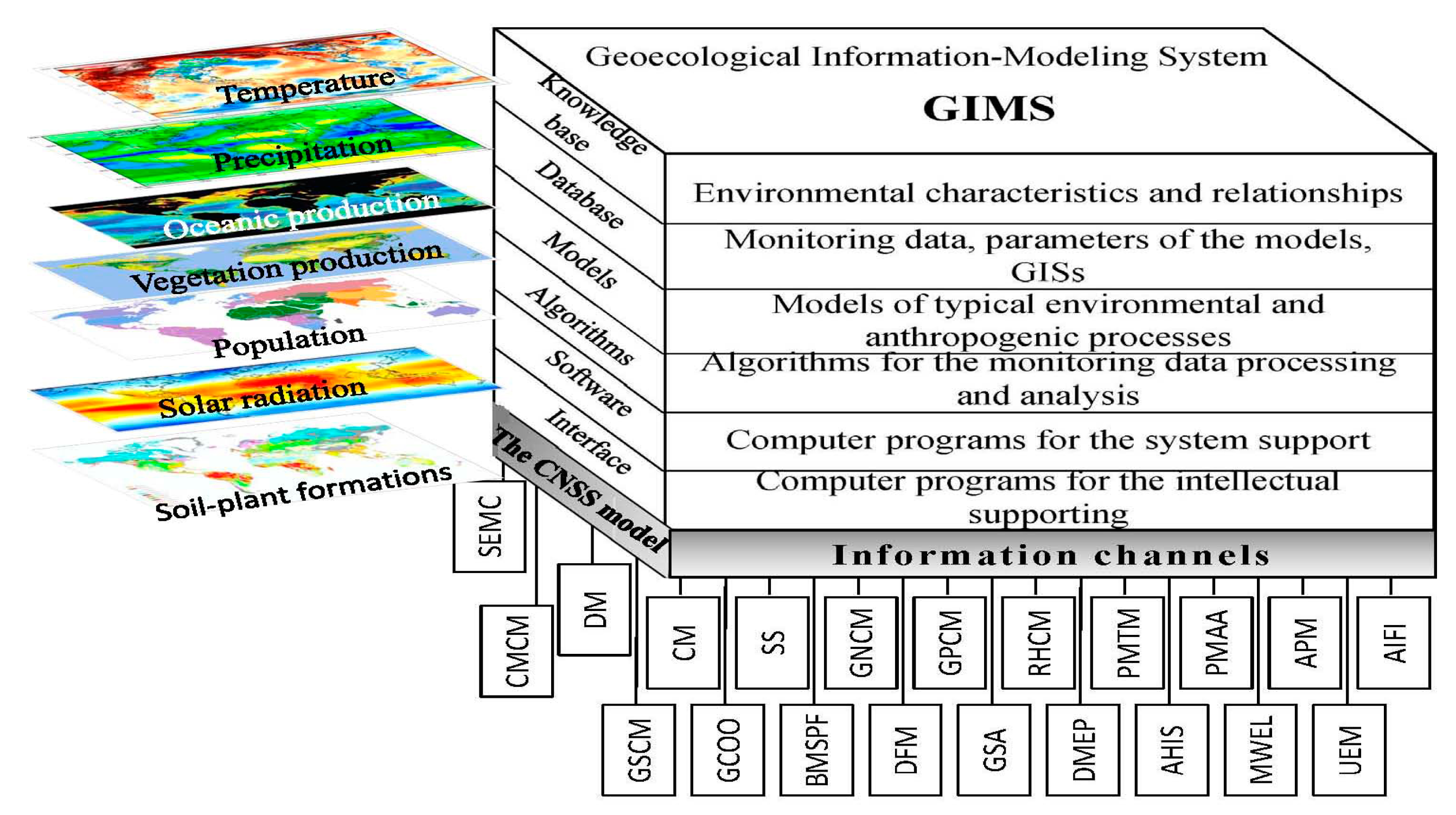
2. General Description of the GIMS/CNSS Model

Key aspect of the assessment of the humanity survivability is the ecological status of the natural evolution of the Earth, which determines food production and other conditions already said. Certainly, the level of self-organization and the structure of the CNSS depends on many factors of the co-evolution of nature-population as elements of the biosphere. Consequently, the composition of the CNSS model is only possible by a synergistic approach that dictates the form and structure of the GIMS/CNSS. GIMS plays a management role by providing coordination between CNSS components and expanding their operations.
Following this approach, the key components of the GIMS/CNSS are defined as the information core for ecological, geophysical, hydrological, biocenotic and demographic processes taking place across the globe. The Earth’s surface Ξ is divided into World Ocean ΞO and the land ΞL (Ξ = ΞL∪ΞO). The land surface ΞL is covered by a geographical grid with discrete steps of Δϕi and Δλj of latitude and longitude, respectively, so that all processes within the pixel ΞLij = {(ϕ, λ): ϕiϕϕi + Δϕi; λjλλj + Δλj} are considered uniform and parameterized by the point models. Each pixel area σij = χϕχλΔϕiΔλj is occupied by the soil-plant formation (r1th part), the agricultural vegetation (r2th part), the hydrophysical objects (r3th part), and the anthropogenic objects ((1−r1r2r3)th part), where χϕ(≈111 km) and χλ(=111.3 cos ϕ) are the number of kilometers to a degree of latitude and longitude, respectively.
In the case of the World Ocean, three latitudinal zones are separated: the equatorial zone ΞO1 = {(ϕ, λ): ϕ∈[0° N, 30° N]∪[0° S, 30° S]; 0° ≤ λ ≤ 360°}, temperate latitudes ΞO2 = {(ϕ, λ): ϕ∈[30° N, 60° N]∪[30°S, 60°S]; 0° ≤ λ ≤ 360°} and Arctic and Antarctic zone ΞO3 = {(ϕ, λ): ϕ∈[60° N, 90° N]∪[60° S, 90° S]; 0° ≤ λ ≤ 360°}. Pelagic ΞO1P and upwelling ΞO1U aquatories are selected in the ΞO1 zone to differ in productivity and gas exchange rate on the air-water boundary [46,47].
Figure 1 and Table 1 show the GIMS/CNSS block structure that is synthesized by taking into account the components and parameters of the global bio-geosystem, managed by geoinformatics monitoring systems. The spatial structure of GIMS/CNSS is defined by the available database and knowledge base. The simplest version of the point model is made when the World Ocean and land are considered as unique element of the planet. The spatial heterogeneity is carried out by the various forms of global space sampling. A basic form of spatial digitization is the choice of a uniform grid Δϕ × Δλ. The GIMS allows the different spatial grids for each CNSS model item that supports the integration of pixels ΞLij. This kind of spatial structure of the biosphere allows the model to be adapted to the heterogeneities of the databases and to perform simulation experiments with the realization of the individual regions.
Depending on the peculiarities of the natural process under consideration, a regional structure can be identified with the climatic and geographic zones, the continents, the natural bio-forms and the socio-administrative structures. For example, Krapivin and Vilkova [48] divided the land’s biosphere into the pixels of magnitude Δϕ = 4° and Δλ = 5°. In more details, the biogeocenotic processes are studied in Δϕ = Δλ = 0.5° [31]; the socio-economic processes are usually represented by three or nine regions, according to the status of the country development [49]; the atmospheric processes in biogeochemical cycles of long-living elements are approached with the point models [50,51]; the functioning of the oceanic ecosystems are represented by the heterogeneous spatial structure including pixels ΞOij of shelf zone and pelagic zones of four oceans [46]. Tarko [52] developed the Moscow Global Biosphere Model, where the World Ocean is represented by the upper quasi-uniform and deep layers separately for four latitudinal zones in the north and south aquatories. It is emphasized that GIMS allows for the combined use of these parameterizations.

3. Description of the GIMS/CNSS Items

The GIMS/CNSS items listed in Table 1 perform the calculations of the energy and matter flows between the spatial digitization pixels of the biosphere taking into account its components. The GIMS/CNSS stability is provided by the information channels linking the functional items so that the change or modification of the item does not affect other items.
Item GSA provides the symbol-parametric identification for pixel components including the soil-plant formations, pollutant sources, water ecosystems and population. As a result, the matrix structures are formed as spatial identifiers of the CNSS elements. Item AHIS focuses on the task of the assessment of the survivability level of population based on available indicators. One of these is the survivability indicator:
J ( t ) = 1 σ { ( i , j ) Ξ L σ i j [ r 1 R Φ 1 ( i , j , t ) R Φ 1 ( i , j , t 0 ) + r 2 R Φ 2 ( i , j , t ) R Φ 2 ( i , j , t 0 ) + r 3 R Φ 3 ( i , j , t ) R Φ 3 ( i , j , t 0 ) ] + s = 1 3 σ O s R P ( s , t ) R P ( s , t 0 ) }
where
R Φ k ( i , j , t ) = R Φ k ( i , j ) min { a C C A ( t ) Γ ( i ) b C + C A ( t ) + Γ ( i ) ,   a E E ( i , t ) b E + E ( i , t ) ,   a W W ( i , j , t ) b W + W ( i , j , t ) , R T ( i , t ) } + M Φ k ( i , j , t ) R T ( i , t ) = max { 0 ,   T ( i , t ) T min ( κ ) T o p t ( κ ) T min ( κ ) exp [ a T b T T ( i , t ) T min ( κ ) T o p t ( κ ) T min ( κ ) ] } , M Φ k ( i , j , t ) = K B Φ k ( i , j ) max { 0 ,   ρ T T ( i , t ) d T + T ( i , t ) ,   d a W ( i , j , t ) d b + W ( i , j , t ) } , T ( i , t ) = T g ( t ) + ( T N ( t ) T e ( t ) ) ( sin 2 ϕ T sin 2 ( 4 i ) ) , R P ( s , t ) = R P s min { Υ 0 ( T W ) ,   Υ 1 ( E ) ,   Υ 2 ( n ) ,   Υ 3 ( P ) } ,   s = 1 , 2 , 3 , Υ 0 ( T W ) = T W T W o p t exp [ θ W ( 1 T W T W o p t ) ] ,   Υ 1 ( E ) = E E max exp [ θ E ( 1 E E max ) ] , Υ 2 ( n ) = [ 1 exp { γ n n ( s , t ) n ( s , t 0 ) } ] θ n ,   Υ 3 ( P ) = 1 exp { γ P P ( s , t ) P ( s , t 0 ) } ,
Table 2 lists the model parameters determined by taking into account the data of separate models from Table 1 and minimizing the disagreement between the pre-historic trends of CO2, the global population size and the relevant model results during 2000–2015. A comparative analysis of the results of the model and of the global temperature trend over the period 2000–2015 showed credibility of the appropriate results at the level of 7–10%.
CA is the CO2 content in the atmosphere (ppmv), E is the solar radiation (W/m2), W is the precipitation (mm/year), TN and Te are the global temperatures at the pole and equator, respectively (°C); Tg is the global average temperature (°C); Tmin and Topt are the critical and optimal temperatures for photosynthesis (°C), respectively [63,64]; ϕT is the latitude at which T(i,t) = Tg; Emax is the solar radiation corresponding to maximal photosynthesis; n is the content of the biogenic salts (mg/m2); P is the phytoplankton biomass (mg/m2); t0(2015) is the starting time, when global average production is assessed by R Φ (2015) = 48.7 PgC/year and R P (2015) = 56.2 PgC/year. Under this R P 1 = 0.049   P g C / day in ΞO3, R P 2 = 0.033   P g C / day in ΞO1, and R P 3 = 0.072   P g C / day in ΞO3 [65,66,67].
Indicator J(t) is an integral feature of the CNSS complexity that reflects the individuality of its structure and its evolution at the time t. According to the laws of natural evolution the decrease or increase of J(t) will reflect the ability of C NSS to survive. Moreover, the reduction of J(t) corresponds to the negative disturbance of the biogeochemical cycles that intensify resource-depletion processes and shift the vector of energetic exchange between the basic functions of the CNSS. In particular, the reduction in J(t) leads to a reduction in total food reserves which may be reflected by the food production index (FDI) which is a function of climate, scientific-technical progress and economic factors [68].
The item CM provides the calculation of the spatial distribution of the mean annual temperature of the atmosphere based on the simple climate model developed by Mintzer [54] and modified by Krapivin et al. [42] as:
ΔTg = ΔTCO2 + ΔTN2O + ΔTCH4 + ΔTO3 + ΔTCFC11 + ΔTCFC12, T(ϕ) = Tg + γ(sin2ϕTsin2ϕ),
where γ is the difference of atmospheric temperatures between the pole and equator, ϕT is the latitude, where T(ϕ) = Tg,
ΔTCO2 = −0.677 + 3.019ln[CА(t)/CА(t*)], ΔTN2O = 0.057[N2O(t)1/2 − N2O(t*)1/2],
ΔTCH4 = 0.019[CH4(t)1/2 − CH4(t*)1/2], ΔTO3 = 0.7[O3(t) − O3(t*)]/15,
ΔTCFC11 = 0.14[CFC11(t) − CFC11(t*)], ΔTCFC12 = 0.16[CFC12(t) − CFC12(t*)].
The value of t* is identified by the year 1980, when the GHG concentration were known (CO2 337.7 ppmv; N2O 270 ppb; CH4 722 ppb; CFC11 167.99 ppb; CFC12 307.75 ppb). Items CMCM, GNCM and GCOO calculate concentrations of CА(t), N2O(t), CH4(t), O3(t) using the corresponding models and CFC11(t), and CFC12(t) taking into account data provided by Butler and Montzka [69].
The item DM refers to the development of a model of population dynamics G(I,j,t) taking into account the environmental factors:
dG(I,j,t)/dt = RG(I,j,t) − MG(I,j,t),
where RG and MG are the indicators of birth rate and mortality, respectively. Birth rate and mortality are mainly functions of the food supply and environmental characteristics. Detailed description of these functions is given in [53].
According to [53] the functions RG(I,j,t) and MG(I,j,t) in (4) are linked to each other with the following equations:
RG(I,j,t) = μBG(I,j,t),
Where μB and μd are the coefficients characterizing the birth rate and mortality, respectively; ϖ is the index of the influence of the population density on mortality. These coefficients are functions of environmental and anthropogenic characteristics, notably:
μB = ρmin{μ1(1 − HDI) + μ2HDI; μ1(1 − HPI) + μ2HPI; μ1exp[−ξ1FPI/FPI(t0)] + μ2[1 − exp{−ξ1FPI/FPI(t0)};
μ1exp[−ξ2GDP/GDP(t0)] + μ2[1 − exp{−ξ2GDP/GDP(t0)}; μ1exp[−ξ3VG] + μ2(1 − exp[−ξ3VG])}
μd = βmin{η1(1 − HDI) + η2HDI; η1(1 − HPI) + η2HPI; η1exp[−χ1FPI/FPI(t0)] + η2[1 − exp{−χ1FPI/FPI(t0)};
η1exp[−χ2GDP/GDP(t0)] + η2[1 − exp{−χ2GDP/GDP(t0)]}; η1exp[−χ3VG] + η2(1 − exp[−χ3VG])}
where μ1 and μ2 are coefficients of maximal and minimal birth rates, respectively; η1 and η2 are maximal and minimal mortalities, respectively; ρ, β, χ1, χ2, χ3, ξ1, ξ2 and ξ3 are adaptation coefficients; VG is the efficient food amount that is defined as weighed sum of the components of personal food spectrum (calculated by the items UEM, PMAA, MWEL, and PMTM).
In the common case we have:
V G ( t ) = { ( i , j ) Ξ L σ i j [ r 1 d 1 R Φ 1 ( i , j , t ) + r 2 d 2 R Φ 2 ( i , j , t ) + + r 3 d 3 R Φ 3 ( i , j , t ) ] + d 4 s = 1 3 R P ( s , t ) } / ( i , j ) Ξ L σ i j G ( i , j , t )
where d1 (0.023), d2 (0.65), d3 (0.11)and d4 (0.013) are coefficients determining the contribution of the production of the natural vegetation, agricultural plants, land water systems and oceans, to the population food spectrum, respectively.
Each pixel Ξij is characterized by the biocomplexity level and participates in the food production as an element of restricted area that can consolidate different biomes, ecosystems and anthropogenic territories. In order to determine the typical description of the spatial structure of CNSS, the following three socio-economic groups of countries are selected to be represented by respective areas of the land ΞL:
-
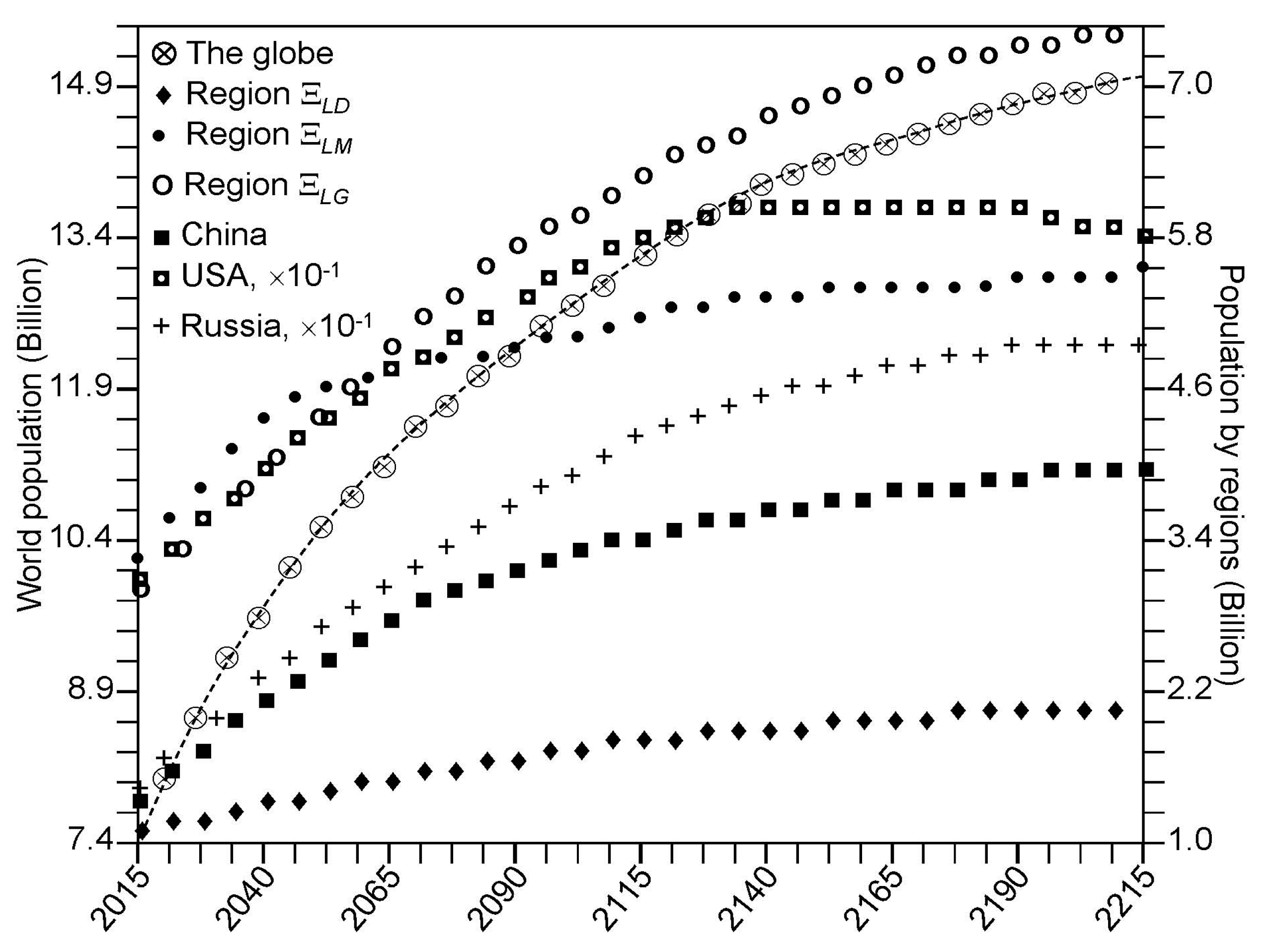
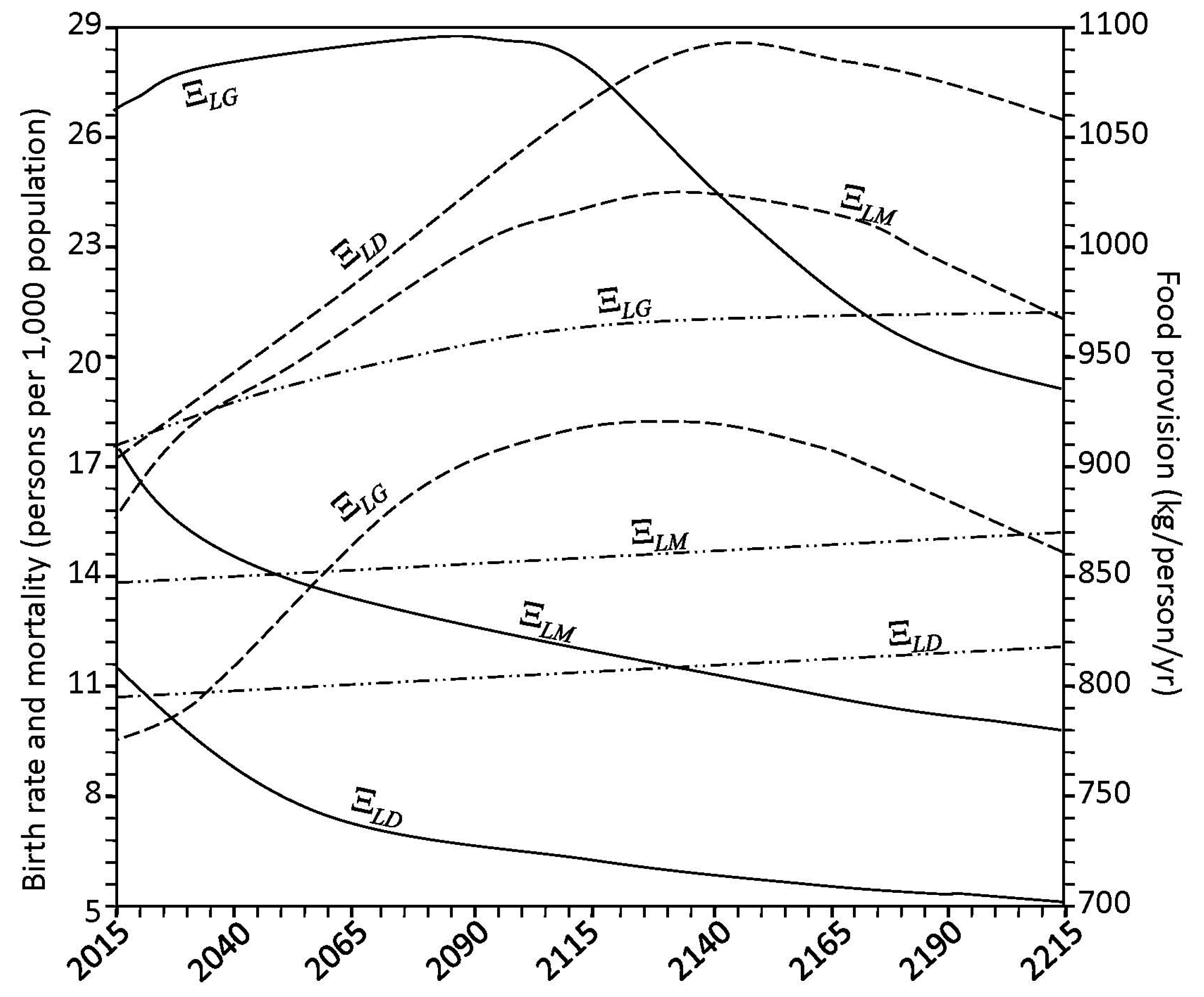
ΞLD the area occupied by countries with HDI ∈ [0.85,1]
-
ΞLM the area occupied by the countries with transition economy (HDI ∈ (0.65,0.85)), and
-
ΞLG correspond to the territory of the developing countries (HDI ∈ [0,0.65]).
Social costs, economic growth, food insecurity, and environmental disruption in each territory are presented with different intensity. The food supply is made from the following available sources:
  • Agricultural technologies are the main food producers that can promote food safety and nutrition security. Global agriculture supplies 2940 kcal per person at present with a forecast of up to 3050 in 2030. Existing protein support per person is estimated at 60 g a day when the medical standard is 70 g. The total protein deficit is estimated at 10 to 25 million tons. Nearly half of the world’s population (7.5 billion) suffers from a lack of protein [70].
  • The second major source of the food is fishing and cultivation of fish in natural lakes and reservoirs. In 2016 each person consumed about 22 kg of fish production. At present, the ecosystems of the World Ocean and the seas provide about 20% of the world’s needs for proteins of animal origin. Mainly, oceanic biomass is estimated around 150 thousands of the animal species and 10 thousands of the water-plants with a total weight of about 35 billion tons which is sufficient to survive 35 billion people [71].
  • Natural plants and forest in the first series can be considered hypothetical sources of food including wild animals and edible plants, hazelnuts, etc. Further development of the food industry and corresponding science allows the expansion of primary use of natural biomass for food production.
As can be seen from Figure 2, Figure 3 and Figure 4, the general trend of food production in various countries is characterized by a steady increase in food production. Practically, in the early 21st century, the majority of countries have achieved comparable levels of the food production. However the problem of the food distribution by the individual has not been solved. This problem is quite complex and is connected with socio-economic and culture-ideological area, the parts of which can be distinguished in cardinals depending on the ideology and the traditional conception of the social justice, whose search is carried out with different indicators [72]. According to the results of Figure 5 and Figure 6, the CNSS space indicator has many uncertainties that can be linked to existing causes of non-uniform distribution of vital resources.
Under the premise of peaceful coexistence, the problem of population survivability lies in providing food to those who have to look after the dependencies of global distribution of food and water supplies on the path of globalization.

4. Simulation Experiments

The GIMS/CNSS allows the emulation of different environmental situations using the information and data that define specific characteristics of the land surface, distribution of the soil-plant formations and hydrosphere. The land surface is covered by a discrete number of land cover types depicted in Figure 7 and Table 3. Numerical values of the GIMS/CNSS parameters are given in Table 4. Certainly, these parameters can change over time, but not significantly. Therefore, the parameters of the regions can be interchanged with each other.
It is clear that the accuracy of a forecast can be estimated only after many years or decades. Nevertheless, a complex set of ideas and assumptions in the GIMS/CNSS structure determine a complete picture of the world and form the mechanisms for constructively describing the direct and inverse relationships in which the CNSS survivability is defined by criterion (1).
The biocomplexity of the environment precisely determines the level of food supply for the world population. As can be seen from Figure 8, a contribution of nature to this conservation has a non-uniform spatial distribution. The corresponding modern spatial distribution is specific for agriculture and fishery productions.
The GIMS/CNSS items that calculate average regional temperature (CM) and simulate regional hydrological balance (RHCM) allow the estimation of surface vegetation production (item BMSPF) depending on temperature and precipitation (a few estimates are given in Table 5).
It will be assumed that the survivability level J(t) is the most important for each region. The GIMS/CNSS forms a comprehensive picture of the population dynamics in the pixel structure of the world and taking into account the respective interactions between the biosphere and climatic system. Undoubtedly, the implementation of GIMS/CNSS that is proposed here improves the structure of existing global models and provides more accurately the calculation of the population dynamics.
The internal resources for each region are determined by the level of Gross Domestic Product (GDP) and its distribution from the strategic goals. The curves in Figure 9 show the dependence of the system survivability on investment distribution and indicate the level of life of the population according to the distribution of GDP by the economic sectors that is correct over the closest limited time period. Overall, the GIMS/CNSS allows evaluation of the population dynamics under certain assumptions. Let’s look at some of them. Figure 10 represents such evaluations in the context of the following assumptions (scenario SP—scientific progress):
  • the problems arising from the limitation of energy sources will be overcome by 2050;
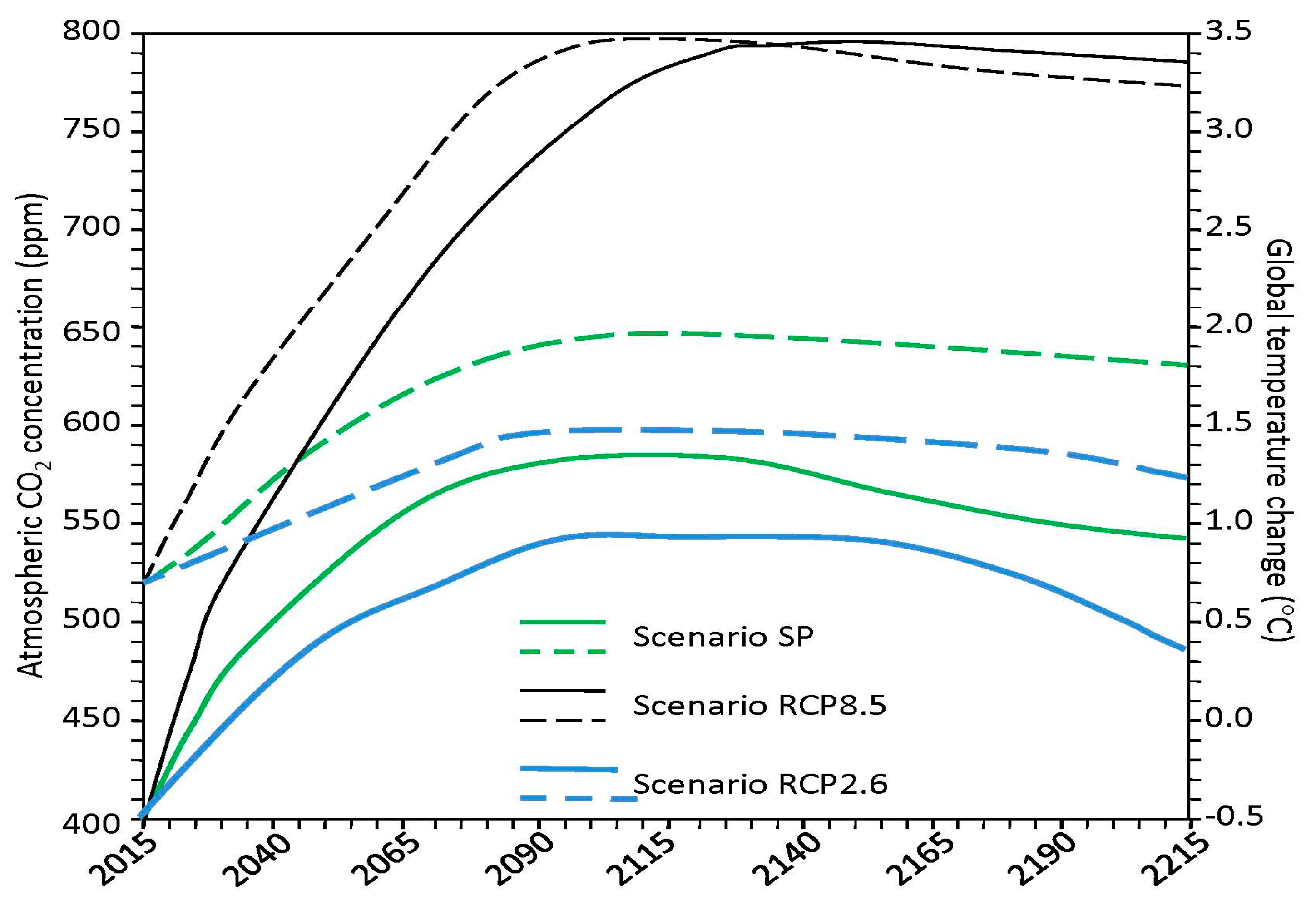
  • the emissions of greenhouse gases will increase by 10% by 2050 compared to 2015 and then begin to fall evenly to 2200 up to 5%;
  • agricultural technologies to increase productivity by 100% by 2050 and by 200% by the end of the 22nd century will be production;
  • the speed of replacement of forest ecosystems by avifauna will be reduced by 10 times in 2050 compared to 2015 and then the forested pixels will not be disturbed; and
  • the contribution of World Ocean resources to food production will increase from 1% in 2015 to 5% in 2050 and then increase steadily to 10% in 2200.
As can be seen from the results of Figure 10, population size can reach 14.9 billion at the beginning of 23rd century with a tendency for low growth. The percentage distribution of the population from the regions will change in the direction of the 6.9% increase in the part of the developing countries. Contributions of the regions ΞLD and ΞLM to population growth declined by 2.1% and 4.8%, respectively. These changes are linked to the different rates of birth and mortality in Equations (6) and (7) as functions of the community status and food supply, as well as climatic parameters. Figure 11 shows some of these characteristics in their dynamics by 2215. It seems that a-priori assumptions about the dynamics of different anthropogenic environmental impacts play an important role in the dynamics of all CNSS components. Unfortunately, these assumptions only occur as specific scenarios.
The implementation of the RCP8.5 scenario (of comparatively high GHS emissions [77]) results in an increase in CO2 concentration to 800 ppm in the 23rd century, beginning with the achievement of a maximal surface temperature increase of almost 3 °C. On the other hand, the fairly realistic scenario RCP2.6 (exploring the possibility of maintaining global mean temperature rise below 2 °C [78]) leads to corresponding levels of 520 ppm for CO2 and 0.8 °C for temperature change in the middle of 22nd century and after lowering these levels. Therefore, the most accurate forecast requires a detailed analysis by the experts of the current trends in the socio-economic developments of the different regions. However, even these hypothetical scenarios provide information to think about the possible safe ways of population growth when survivability is maintained for a long time.
Figure 12 shows a dynamics of the key factors that are linked with evolution process of the society development. The birth rate coefficients μB for the ΞLD, ΞLM and ΞLG regions are change from 0.0115, 0.0177 and 0.0267 in 2015 to 0.005, 0.0098 and 0.0191 in 2200, respectively. According to this, the birth rate coefficients of the ΞLD and ΞLM regions will decrease evenly with time, and the birth rate coefficient will reach the maximal value 0.034 in the ΞLG region in 2060 and then decrease. The mortality coefficients μd are similarly modified in the ΞLD, ΞLM and ΞLG regions from 0.0107, 0.0138 and 0.0175 in 2015, to 0.0121, 0.0153 and 0.0211 in 2200, respectively.

5. Conclusions

The proposed version of the global geo-ecological information-modeling system provides tools for studying and evaluating the limiting anthropogenic impacts on the biosphere and allows for the understanding of its responses and identification of the exclusion area for possible human activity. In this context, the GIMS/CNSS provides the capability to detect regional ecological responses to the effects identified in the limited number of spatial pixels. The GIMS/CNSS is based on combined use of specific models of particular environmental processes listed in Table 1 and tested separately. The parameters of the model such as ρ, β, χ1, χ2, χ3, ξ1, ξ2 and ξ3 are corrected, based on the minimal discrepancy between modeling results and the prehistory of trends in the global population and atmospheric CO2 during 2000–2015. The model verification is based on a comparison of the prehistory trends of the real global temperature with those deduced by the model. In this case the average deviation for the period 2000–2015 was no more 7%.
The GIMS/CNSS can be used to evaluate the consequences of the implementation of anthropogenic scenarios, such as spatial reconstruction of soil-plant formations or changes in the vegetation cover as a result of wildfires. The modelled changes are accomplished by replacing literal symbols in the map of the soil-plant formations (Figure 7). Preliminary calculations have shown a strong dependence of the CO2 cycle [79,80] on changes in vegetation cover.
Undoubtedly, the GIMS/CNSS reflects the limited range of feedbacks in CNSS with emphasis on ecological interactions. The GIMS/CNSS allows the modernization its structure through additional items that shape the socio-economic and living feedbacks in the global climate system.
It should be noted that the GIMS/CNSS Global Model developed here is not comparable to other available complex global models. The model of global environmental processes based on the GIMS-technology differs largely from other global models from the ability to evolutionary adapt to pre-history using informative indicators on the state of CNSS. Certainly, the adaptation process and the selection of informative indicators are needed in the additional surveys.
The results of this study show that survivability problem will not be critical over the next two centuries, depending on the population growth. Restrictions on the availability of food production resources will occur at the end of 21st century when, as shown in Figure 12, the global nuclear power plant (NPP) is slowly declining due to climate change and changes in regional hydrological balances. In particular, the rise in temperature in tropical latitudes causes a decrease in water content in the soil due to the evaporation which leads to the NPP decrease. In contrast, in northern pixels, the rise in temperature leads to a 16–20 day extension in the 22nd century, starting with a 9–12% increase in the NPP. These negative and positive feedbacks are not evenly distributed by the pixels. As a result, the food production dynamics illustrated in Figure 12 shows that the export of excess of food stocks of the region ΞLG to other regions is only possible until the end of 21st century, as the human population expands the effectiveness of such strategies, such as expansion of the land area used for agriculture, the expansion of fishing, and the increase in agricultural productivity. Current trends in increasing the regional population suggest that satisfying food demands is unlikely to occur if human society does not seek sustainable interactions with nature. Realized food production estimates are approximate and can be more accurate when spatial digitization of land and oceans will be, for example, 0.5° × 0.5° or less. It is known that changes in net primary production in the ocean vary from 1800 g/m2/year in estuaries to 50 g/m2/year in the open ocean. Biomass variations and biomass production of the land vegetation have a wide range as well. This circumstance is an additional reserve to make the results of the global model more accurate. Certainly, the GIMS/CNSS model allows for a more detailed description of the soil-plant formations depicted in Figure 7 taking into account the existing site variations and productivity, as well as the specifications of agricultural ecosystems. Additional enlargement and identification of global and regional environmental databases are required. Furthermore, the analysis presented showed that all the given assumptions are closely related to the results of the presented model. In addition, the potential use of the presented model at regional and global level is presented in [22,23,46,47]. It would be of particular interest to apply this model to investigate the impact on public health from modern environmental problems, such as the depletion of the ozone layer and the induced increase in solar ultraviolet radiation reaching the ground [81,82,83,84,85,86,87].

Author Contributions

Vladimir F. Krapivin and Costas A. Varotsos conceived and designed the experimental application and validation of the NSS, CNSS and GIMS/CNSS models; Vladimir Yu. Soldatov performed the simulation experiments.

Conflicts of Interest

The authors declare no conflict of interest.

References

  1. Varotsos, C.A.; Franzke, C.L.; Efstathiou, M.N.; Degermendzhi, A.G. Evidence for two abrupt warming events of SST in the last century. Theor. Appl. Climatol. 2014, 116, 51–60. [Google Scholar] [CrossRef]
  2. Kondratyev, K.Y.; Varotsos, C. Atmospheric greenhouse effect in the context of global climate change. Nuovo Cimento C 1995, 18, 123–151. [Google Scholar] [CrossRef]
  3. Varotsos, C.A. The global signature of the ENSO and SST-like fields. Theor. Appl. Climatol. 2013, 113, 197–204. [Google Scholar] [CrossRef]
  4. Varotsos, C.; Assimakopoulos, M.N.; Efstathiou, M. Long-term memory effect in the atmospheric CO2 concentration at Mauna Loa. Atmos. Chem. Phys. 2007, 7, 629–634. [Google Scholar] [CrossRef]
  5. Efstathiou, M.N.; Varotsos, C.A. On the altitude dependence of the temperature scaling behaviour at the global troposphere. Int. J. Remote Sens. 2010, 31, 343–349. [Google Scholar] [CrossRef]
  6. Efstathiou, M.N.; Tzanis, C.; Cracknell, A.P.; Varotsos, C.A. New features of land and sea surface temperature anomalies. Int. J. Remote Sens. 2011, 32, 3231–3238. [Google Scholar] [CrossRef]
  7. Efstathiou, M.N.; Varotsos, C.A. Intrinsic properties of Sahel precipitation anomalies and rainfall. Theor. Appl. Climatol. 2012, 109, 627–633. [Google Scholar] [CrossRef]
  8. Varotsos, C.A.; Efstathiou, M.N.; Cracknell, A.P. On the scaling effect in global surface air temperature anomalies. Atmos. Chem. Phys. 2013, 13, 5243–5253. [Google Scholar] [CrossRef]
  9. Mayhew, R.J. (Ed.) New Perspectives on Malthus; Cambridge University Press: Cambridge, UK, 2016. [Google Scholar]
  10. Shaw, P. A Treatise of Incurable Diseases; BiblioBazaar: Charleston, SC, USA, 2010. [Google Scholar]
  11. Okazaki, K. Good-Bye Incurable Diseases! iUniverse, Inc.: Bloomington, IN, USA, 2011. [Google Scholar]
  12. Weart, S.R. The Discovery of Global Warming; Harvard University Press: Harvard, MA, USA, 2008. [Google Scholar]
  13. Cimbala, S.J. Nuclear Weapons in the Information Age; Continuum International Publishing Group: London, UK, 2012. [Google Scholar]
  14. Daun, H. (Ed.) School decentralization in the context of globalizing governance. In International Comparison of Grassroots Responses; Springer: Dordrecht, The Netherlands, 2007. [Google Scholar]
  15. Sahib, S.S. Impact of mobile phones on the density of honeybees. J. Publ. Admin. Pol. Res. 2011, 3, 131–133. [Google Scholar]
  16. Anderson, B.A. World Population Dynamics: An Introduction to Demography; Pearson Publ. Ltd.: Cambridge, UK, 2015. [Google Scholar]
  17. Berthelot, M.; Friedlingstein, P.; Ciais, P.; Monfray, P. Global response of the terrestrial biosphere to CO2 and climate change using a coupled climate-carbon cycle model. Glob. Biogeochem. Cycles 2002, 16, 31. [Google Scholar] [CrossRef]
  18. Dufresne, J.-L.; Foujols, M.-A.; Denvil, S.; Caubel, A.; Marti, O. Climate change projections using the IPSL-CM5 Earth System Model: From CMIP3 to CMIP5. Clim. Dyn. 2013, 40, 2123–2165. [Google Scholar] [CrossRef] [Green Version]
  19. Kondratyev, K.Y.; Krapivin, V.F.; Phillips, G.W. Arctic Basin pollution dynamics. In Arctic Environment Variability in the Context of Global Change; Bobylev, L.P., Kondratyev, K.Y., Johannesses, O.M., Eds.; Springer: Chichester, UK, 2003; pp. 309–362. [Google Scholar]
  20. Kondratyev, K.Y.; Krapivin, V.F.; Varotsos, C.A. Global Carbon Cycle and Climate Change; Springer: Chichester, UK, 2003. [Google Scholar]
  21. Krapivin, V.F.; Varotsos, C.A. Globalization and Sustainable Development; Springer: Chichester, UK, 2007; 304p. [Google Scholar]
  22. Krapivin, V.F.; Varotsos, C.A. Biogeochemical Cycles in Globalization and Sustainable Development; Springer: Chichester, UK, 2008. [Google Scholar]
  23. Krapivin, V.F.; Varotsos, C.A.; Soldatov, V.Y. New Ecoinformatics Tools in Environmental Science: Applications and Decision-Making; Springer: London, UK, 2015. [Google Scholar]
  24. Moisseev, N.N. Mathematics Produces an Experiment; Science Publ.: Moscow, Russia, 1979; 223p. (In Russian) [Google Scholar]
  25. Forrester, J.W. World Dynamics; Wright-Allen Press: Cambridge, MA, USA, 1971. [Google Scholar]
  26. Forrester, J.W. World Dynamics; Productivity Press Publishing: New York, NY, USA, 1979. [Google Scholar]
  27. Meadows, D.H.; Meadows, D.L.; Randers, J.; Behrens, W.W., III. The Limits to Growth; Universe Books: New York, NY, USA, 1972. [Google Scholar]
  28. Meadows, D.H.; Randers, J.; Meadows, D.L. Limits of Grows: The 30-Years Update; Chelsea Green Publishing: White River Junction, VT, USA, 2004. [Google Scholar]
  29. Pestel, E. Beyond the Limits to Growth: A Report to Club of Rome; Universe Books: New York, NY, USA, 1989. [Google Scholar]
  30. Krapivin, V.F. Mathematical model for global ecological investigations. Ecol. Model. 1993, 67, 103–127. [Google Scholar] [CrossRef]
  31. Sellers, P.J.; Los, S.O.; Tucker, C.J.; Justice, C.O.; Dazlich, D.A.; Collatz, G.J.; Randall, D.A. A revised land surface parametrization (SiB2) for atmospheric GCMs. Part II: The generation of global fields of terrestrial biophysical parameters from satellite data. J. Clim. 1996, 9, 708–737. [Google Scholar]
  32. Degermendzhi, A.G. New directions in biophysical ecology. In Global Climatology and Ecodynamics; Cracknell, A.P., Krapivin, V.F., Varotsos, C.A., Eds.; Springer: Chichester, UK, 2009; pp. 379–396. [Google Scholar]
  33. Degermendzhi, A.G.; Bartsev, S.I.; Gubanov, V.G.; Erokhin, D.V.; Shevirnogov, A.P. Forecast of biosphere dynamics using small-scale models. In Global Climatology and Ecodynamics; Cracknell, A.P., Krapivin, V.F., Varotsos, C.A., Eds.; Springer: Chichester, UK, 2009; pp. 241–300. [Google Scholar]
  34. Krapivin, V.F.; Kelley, J.J. Model-based method for the assessment of global change in a nature-society system. In Problems of Global Climatology and Ecodynamics; Cracknell, A.P., Krapivin, V.F., Varotsos, C.A., Eds.; Springer: Chichester, UK, 2009; pp. 133–184. [Google Scholar]
  35. Saavedra-Rivano, N. A critical analysis of the Mesarovic-Pestel world model. Appl. Math. Model. 1979, 3, 384–390. [Google Scholar] [CrossRef]
  36. Vernadsky, W.I. Problems of biogeochemistry II. Trans. Conn. Acad. Arts Sci. 1944, 35, 493–494. [Google Scholar]
  37. Xue, Y.; Sellers, P.J.; Kinter, J.L.; Shukla, J. A simplified biosphere model for global climate studies. J. Clim. Am. Meteorol. Soc. 1991, 4, 345–364. [Google Scholar] [CrossRef]
  38. Ondov, J.M.; Buckley, T.J.; Hopke, P.K.; Ogulei, D.; Parlange, M.B.; Rogge, W.F.; Squibb, K.S.; Johnston, M.V.; Wexler, A.S. Baltimore Supersite: Highly time- and size-resolved concentrations of urban PM2.5 and its constituents for resolution of sources and immune responses. Atmos. Environ. 2006, 40, 224–237. [Google Scholar] [CrossRef]
  39. Xue, Y.; He, X.W.; Xu, H.; Guang, J.; Guo, J.P.; Mei, L.L. China Collection 2.0: The aerosol optical depth dataset from the synergetic retrieval of aerosol properties algorithm. Atmos. Environ. 2014, 95, 45–58. [Google Scholar] [CrossRef]
  40. Ebel, A.; Memmesheimer, M.; Jakobs, H.J. Chemical perturbations in the planetary boundary layer and their relevance for chemistry transport modelling. Bound.-Lay. Meteorol. 2007, 125, 265–278. [Google Scholar] [CrossRef]
  41. Chattopadhyay, G.; Chakraborthy, P.; Chattopadhyay, S. Mann-Kendall trend analysis of tropospheric ozone and its modeling using ARIMA. Theor. Appl. Climatol. 2012, 110, 321–328. [Google Scholar] [CrossRef]
  42. Krapivin, V.F.; Mkrtchyan, F.A.; Van, T.D. Constructive method for the vegetation microwave monitoring. In Proceedings of the International Symposium on Engineering Ecology, Moscow, Russia, 2–4 December 2015; The Russian Sciences Engineering A.S. Popov Society for Radio, Electronics and Communication: Moscow, Russia, 2015; pp. 21–27. [Google Scholar]
  43. Krapivin, V.F.; Mkrtchyan, F.A.; Nazaryan, N.A. Development of GIMS-technology for environmental monitoring of ocean ecosystems. In Proceedings of the 31st International Symposium on Okhotsk Sea & Sea Ice, Mombetsu, Hokaido, Japan, 21–24 February 2016; The Okhotsk Sea & Polar Oceans Research Association: Mombetsy, Hokkaido, Japan, 2016; pp. 116–119. [Google Scholar]
  44. Nitu, C.; Krapivin, V.F.; Bruno, A. Intelligent Techniques in Ecology; Printech: Bucharest, Romania, 2000. [Google Scholar]
  45. Pawłowski, A. Sustainable development as a civilizational revolution. In A Multidisciplinary Approach to the Challenges of the 21st Century; CRC Press: New York, NY, USA, 2011. [Google Scholar]
  46. Krapivin, V.F.; Varotsos, C.A. Modelling the CO2 atmosphere-ocean flux in the upwelling zones using radiative transfer tools. J. Atmos. Sol.-Terr. Phys. 2016, 150–151, 47–54. [Google Scholar] [CrossRef]
  47. Krapivin, V.F.; Varotsos, C.A.; Soldatov, V.Y. Simulation results from a coupled model of carbon dioxide and methane global cycles. Ecol. Model. 2017, 359, 69–79. [Google Scholar] [CrossRef]
  48. Krapivin, V.F.; Vilkova, L.P. Model estimation of excess CO2 distribution in biosphere structure. Ecol. Model. 1990, 50, 57–78. [Google Scholar] [CrossRef]
  49. Korotaev, A.; Zinkina, J. On the structure of the present-day convergence. Campus-Wide Inf. Syst. 2014, 31, 139–152. [Google Scholar] [CrossRef]
  50. Nitu, C.; Krapivin, V.F.; Pruteanu, E. Ecoinformatics: Intelligent Systems in Ecology; Magic Print Onesti: Bucharest, Romania, 2004. [Google Scholar]
  51. Nitu, C.; Krapivin, V.F.; Soldatov, V.Y. Information-Modeling Technology for Environmental Investigations; Matrix Rom: Bucharest, Romania, 2013. [Google Scholar]
  52. Tarko, A.M. Analysis of Global and Regional Changes in Biogeochemical Carbon Cycle: A Spatially Distributed Model; IR-03-041; IIASA, Inter. Rep.: Laxenburg, Austria, 2003. [Google Scholar]
  53. Kondratyev, K.Y.; Krapivin, V.F.; Savinykh, V.P.; Varotsos, C.A. Global Ecodynamics: A Multidimensional Analysis; Springer: Chichester, UK, 2004. [Google Scholar]
  54. Mintzer, I.M. A Matter of Degrees: The Potential for Controlling the Greenhouse Effect; World Resources Institute: Washitong, DC, USA, 1987. [Google Scholar]
  55. Varotsos, C.A.; Krapivin, V.F.; Soldatov, V.Yu. Modeling the carbon and nitrogen cycles. Front. Environ. Sci. Air Pollut. 2014, 2. [Google Scholar] [CrossRef]
  56. Kondratyev, K.Y.; Ivlev, L.S.; Krapivin, V.F.; Varotsos, C.A. Atmospheric Aerosol Properties: Formation, Processes and Impacts; Springer: Chichester, UK, 2006. [Google Scholar]
  57. Krapivin, V.F.; Shutko, A.M. Information Technologies for Remote Monitoring of the Environment; Springer: Chichester, UK, 2012. [Google Scholar]
  58. Krapivin, V.F. The estimation of the Peruvian current ecosystem by a mathematical model of biosphere. Ecol. Model. 1996, 91, 1–14. [Google Scholar] [CrossRef]
  59. Kondratyev, K.Y.; Krapivin, V.F.; Phillips, G.W. High Latitude Environmental Pollution Problems; Cankt-Petersburg State University Publ.: Sankt-Petersburg, Russia, 2002. [Google Scholar]
  60. Krapivin, V.F.; Mkrtchyan, F.A.; Soldatov, V.Y. Simulation model of the Arctic Basin ecosystem. In Proceedings of the 32nd International Symposium on Okhotsk Sea & Polar Oceans, Mombetsu, Hokkaido, Japan, 19–22 February 2017; Okhotsk Sea and Polar Oceans Research Association: Mombetsu, Hokkaido, Japan, 2017; pp. 337–340. [Google Scholar]
  61. Van Tuyet, D.; Man, N.X.; Van, L.T.T.; Krapivin, V.F.; Mkrtchyan, F.A.; Hung, N.T.; Thanh, L.N. Global model of carbon cycle as instrument of primary agriculture production assessment. In Proceedings of the International Symposium “Some Aspects of Contemporary Issues in Ecoinformatics”, Hochiminh City, Vietnam, 20 March 2015; Institute of Applied Mechanics and Informatics, Vietnam Academy of Science and Technology: Hochiminh City, Vietnam, 2015; pp. 50–58. [Google Scholar]
  62. Nitu, C.; Dumitrasku, A.; Krapivin, V.F.; Mkrtchyan, F.A. Reducing risks in agriculture. In Proceedings of the 20th International Conference on Control Systems and Computer Science, Bucharest, Romania, 27–29 May 2015; University Politehnica of Bucharest Campus: Bucharest, Romania, 2015; pp. 941–945. [Google Scholar]
  63. Kaduk, J.; Heimann, M. A prognostic phenology scheme for global terrestrial carbon cycle models. Clim. Res. 1996, 6, 1–19. [Google Scholar] [CrossRef]
  64. Hatfield, J.L.; Prueger, J.H. Temperature extremes: Effect on plant growth and development. Weather Clim. Extrem. 2015, 10, 4–10. [Google Scholar] [CrossRef]
  65. Coupel, P.; Ruiz-Pino, D.; Sicre, M.A.; Chen, J.F.; Lee, S.H.; Schiffrine, N.; Li, H.L.; Gascard, J.C. The impact of freshening on phytoplankton production in the Pacific Arctic Ocean. Prog. Oceanogr. 2015, 131, 113–125. [Google Scholar] [CrossRef] [Green Version]
  66. Burford, M.A.; Rothlisberg, P.C. Factors limiting phytoplankton production in a tropical continental shelf ecosystem estuarine. Coast. Shelf Sci. 1999, 48, 541–549. [Google Scholar] [CrossRef]
  67. Raymont, J.E.G. Plankton and Productivity in the Oceans; Vol. 1: Phytoplankton; Pergamon Press: New York, NY, USA, 1980. [Google Scholar]
  68. Alexandratos, N.; Bruinsma, J. World Agriculture Forwards 2030/2050; FAO: Rome, Italy, 2012. [Google Scholar]
  69. Butler, J.H.; Montzka, S.A. The NOAA Annual Greenhouse Gas Index (AGGI); NOAA Earth System Research Laboratory, Global Monitoring Division. Available online: www.esrl.noaa.gov/gmd/aggi/aggi.html (accessed on 6 August 2017).
  70. Debertin, D.L. Agricultural Production Economics; Macmillan Publish Company: London, UK, 2012. [Google Scholar]
  71. Lucas, J.S.; Southgate, P.C. Aquaculture: Farming Aquatic Animals and Plants; John Wiley and Sons: New York, NY, USA, 2012. [Google Scholar]
  72. Card, D.; Raphael, S. Immigration, Poverty, and Socioeconomic Inequality; Russel Sage Foundation: New York, NY, USA, 2013. [Google Scholar]
  73. Dixon, A.P.; Faber-Langendoen, D.; Josse, C.; Morrison, J.; Loucks, C.J. Distribution mapping of world grassland types. J. Biogeogr. 2014, 41, 2003–2019. [Google Scholar] [CrossRef]
  74. Shvidenko, A.Z.; Schepaschenko, D.C.; Nilsson, S.; Buluy, Y.I. Tables and Models of Growth and Productivity of Forests of Major Forest Forming Species of Northern Eurasia; Federal Agency of Forest Management: Moscow, Russia, 2008. [Google Scholar]
  75. Riahi, K.; Krey, V.; Rao, S.; Chirkov, V.; Fischer, G.; Kolp, P.; Kindermann, G.; Nakicenovic, N.; Rafai, P. RCP-8.5: Exploring the consequence of high emission trajectories. Clim. Chang. 2011, 109. [Google Scholar] [CrossRef]
  76. Van Vuuren, D.P.; Stehfest, E.; den Elzen, M.G.J.; Kram, T.; van Vliet, J.; Deetman, S.; Isaac, M.; Goldewijk, K.K.; Hof, A.; Beltran, A.M.; et al. RCP2. 6: Exploring the possibility to keep global mean temperature increase below 2 C. Clim. Chang. 2011, 109. [Google Scholar] [CrossRef]
  77. Li, J.; Mao, J. Changes in the boreal summer intraseasonal oscillation projected by the CNRM-CM5 model under the RCP 8.5 scenario. Clim. Dyn. 2016, 47, 3713–3736. [Google Scholar] [CrossRef]
  78. Wayne, G.P. The beginner’s guide to representative concentration pathways. Scept. Sci. 2013, 25. Available online: http://denning.atmos.colostate.edu/ats760/Readings/RCP_Guide.pdf (accessed on 6 August 2017).
  79. Varotsos, C. Solar ultraviolet radiation and total ozone, as derived from satellite and ground-based instrumentation. Geophys. Res. Lett. 1994, 21, 1787–1790. [Google Scholar] [CrossRef]
  80. Varotsos, C. Climate change problems and carbon dioxide emissions: Expecting ‘Rio + 10’. Environ. Sci. Pollut. Res. 2002, 9, 97–98. [Google Scholar] [CrossRef]
  81. Cracknell, A.P.; Varotsos, C.A. Ozone depletion over Scotland as derived from Nimbus-7 TOMS measurements. Int. J. Remote Sens. 1994, 15, 2659–2668. [Google Scholar] [CrossRef]
  82. Cracknell, A.P.; Varotsos, C.A. The present status of the total ozone depletion over Greece and Scotland: A comparison between Mediterranean and more northerly latitudes. Int. J. Remote Sens. 1995, 16, 1751–1763. [Google Scholar] [CrossRef]
  83. Varotsos, C.; Kalabokas, P.; Chronopoulos, G. Association of the laminated vertical ozone structure with the lower-stratospheric circulation. J. Appl. Meteorol. 1994, 33, 473–476. [Google Scholar] [CrossRef]
  84. Varotsos, C. The southern hemisphere ozone hole split in 2002. Environ. Sci. Pollut. Res. 2002, 9, 375–376. [Google Scholar] [CrossRef]
  85. Varotsos, C.; Cartalis, C. Re-evaluation of surface ozone over Athens, Greece, for the period 1901–1940. Atmos. Res. 1991, 26, 303–310. [Google Scholar] [CrossRef]
  86. Varotsos, C.A.; Cracknell, A.P. Ozone depletion over Greece as deduced from Nimbus-7 TOMS measurements. Int. J. Remote Sens. 1993, 14, 2053–2059. [Google Scholar] [CrossRef]
  87. Varotsos, C. Airborne measurements of aerosol, ozone, and solar ultraviolet irradiance in the troposphere. J. Geophys. Res.-Atmos. 2005, 110, D09202. [Google Scholar] [CrossRef]
Figure 1. The GIMS/CNSS block-diagram. Abbreviation expansion is given in Table 1.
Ijerph 14 00885 g001
Figure 2. Food production indicators in major countries.
Ijerph 14 00885 g002
Figure 3. Comparison of food production indicators for developed and developing countries.
Ijerph 14 00885 g003
Figure 4. Comparison of food production indicators in developed countries and weakly developed countries.
Ijerph 14 00885 g004
Figure 5. Birth rates and mortality dependencies on the Human Development Index adopted by the countries.
Ijerph 14 00885 g005
Figure 6. An interdependence of the Food Production Index (FPI) and Human Development Index (HDI) for the different countries.
Ijerph 14 00885 g006
Figure 7. Spatial distribution of the types of soil-plant formations presented in Table 3. Biome indicator is explained in Table 3.
Ijerph 14 00885 g007
Figure 8. A map-scheme of the productivity of soil-plant formations shown in Table 2 in digital scale with spatial resolution 4° × 5°.
Ijerph 14 00885 g008
Figure 9. Survivability indicator depending on the GDP distribution by agriculture (solid lines) and industry (dashed lines). Numbers located on the right of the curves show the time periods for the investments: 1–25 years, 2–50 years, 3–75 years, and 4–100 years.
Ijerph 14 00885 g009
Figure 10. The global and regional population dynamics.
Ijerph 14 00885 g010
Figure 11. The dynamics of the climatic factors (CO2 concentration and temperature are represented by the solid and dashed lines, respectively). A comparison of the results obtained from the implementation of the SP scenario with those from the RCP8.5 and RCP2.6 scenarios [75,76].
Ijerph 14 00885 g011
Figure 12. The dynamics of the vital factors (supply of food by region, birth rate, and mortality are represented by the broken, solid, and chain lines, respectively). Regional identifiers are placed on the curves.
Ijerph 14 00885 g012
Table 1. The GIMS/CNSS functional items.
ItemItem Functions
DMDemographic model [53].
CMClimate model [42,54].
CMCMCoupled model of the carbon dioxide and methane cycles [47].
GSCMGlobal sulphur cycle model [22].
GCOOCoupled model of global cycles of oxygen and ozone [22].
GNCMGlobal nitrogen cycle model [55].
GPCMGlobal phosphorus cycle model [56].
RHCMRegional hydrological cycle model [57].
BMSPFBiocenotic model of the soil-plant formations [48,50].
PMTMPhotosynthesis model for the tropical and moderate oceanic zones [58].
PMAAPhotosynthesis model for the Arctic and Antarctic zones of the World Ocean [19,59,60].
APMAgriculture production model [61,62].
AIFIEvolutionary algorithm for the indicator calculation of the food industry [44,50].
UEMAn upwelling ecosystem model [46].
MWELModel of the typical water ecosystem on the land [57].
AHISAn algorithm for the human indicator survivability calculation.
DMEPDynamic model of the environmental pollutants [56].
GSAThe GIMS structure adaptation to the simulation experiment conditions [23,42].
DFMDatabase formation and management.
SSSynthesis of the scenarios for the interaction of population with the environment.
SEMCSimulation experiment management and control.
Table 2. List of the model parameters.
ParameterSymbolParameter Evaluation
Photosynthesis compensation constant: Γ, ppmv
Equator5
Pole50
Coefficient reflecting the effect of the CO2 factor on plant production.aC3.226
Constant of the photosynthetic responses to atmospheric CO2 changes.bC, ppmv930.03
Coefficient reflecting the impact of solar radiation on plant production.aE1.177
Parameter indicating the solar radiation in which the stability of plant production is achieved.bE, W/m260.538
Coefficient reflecting the effect of precipitation on plant production.aW4.742
Parameter indicating the precipitation in which the stability of plant production is achieved.bW mm/year592.357
Parameter indicating the maximal rate of growth of plant biomass under temperature change.aT0.56
Indicator of declining plant production under temperature change.bT0.42
Maximal rate of loss of plant biomass under temperature change.ρT1.214
Parameter that controls early delay to achieve a maximal rate of loss of plant biomass due to temperature change.dT, °C5.714
Maximal rate of loss of plant biomass under change of soil moisture. da0.0267
Parameter that controls early delay to achieve a maximal rate of loss of plant biomass to precipitation change.db, mm/year208.333
Ratio coefficient that characterizes phytoplankton rate dependence on temperature.θW0.21
Ratio coefficient that characterizes phytoplankton rate dependence on solar energy.θE0.25
Constant that determines the characteristics of phytoplankton species dependent on biogenic salts.γN0.1
Constant that determines phytoplankton production as a function of its biomass.γP0.25
The area of the biosphere.σ, km2510.1 × 106
Model start time.t02015
Table 3. Quantitative characteristics of the formation types of the land vegetation [60,63,73,74]. Notation: σS is the biome area (mln km2), R Φ 1 is the annual increment of plants (kg/m2/year), Φ* is the phytomass (kg/m2). Tmin and Topt are minimal and optimal temperatures for photosynthesis, respectively.
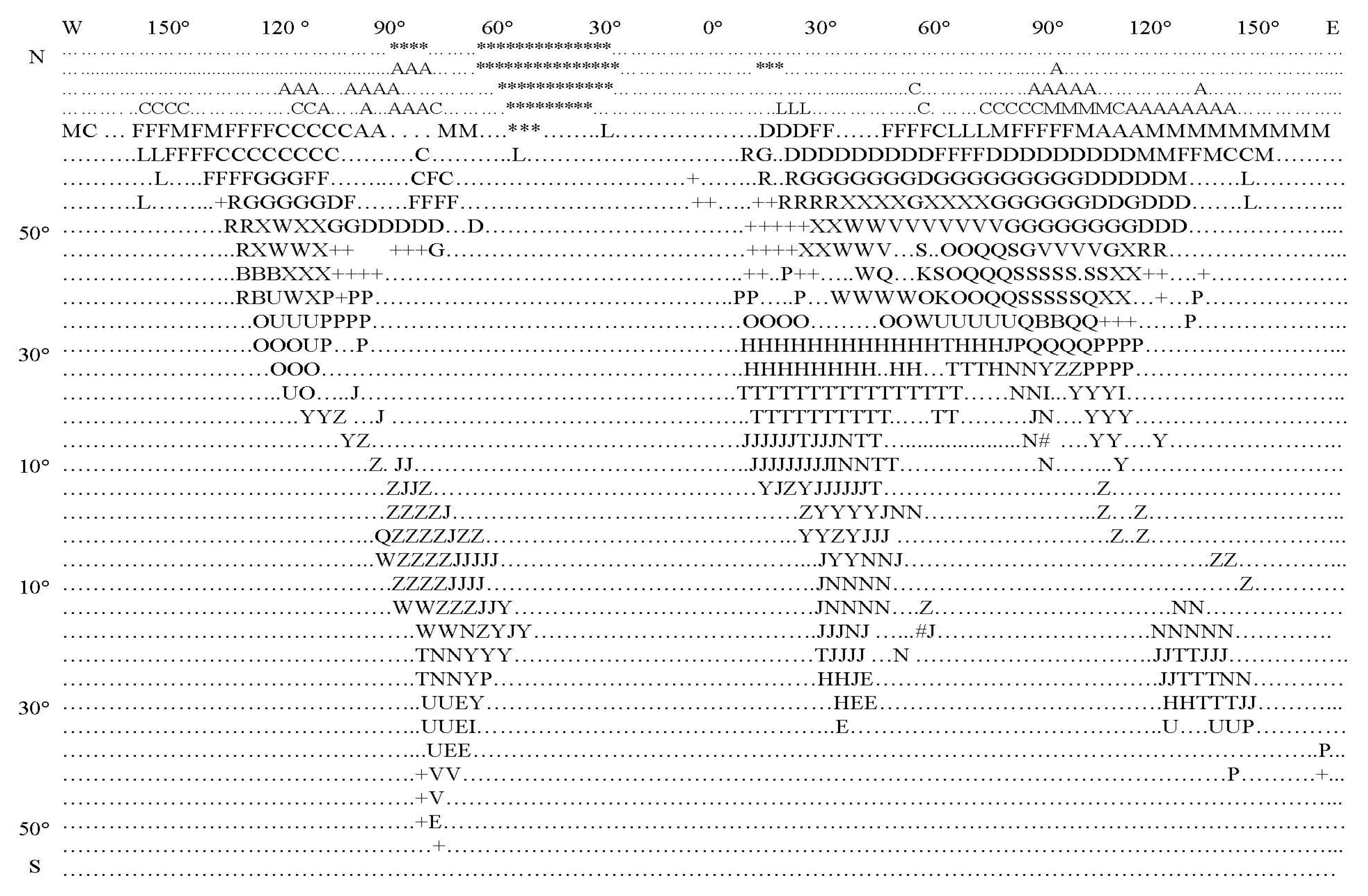
Indicator and Type of Soil-Plant FormationσS R Φ 1 Φ*Tmin (°C)Topt (°C)
A—Arctic deserts and tundra2.550.170.4−540
C—Tundra2.930.361.9−540
M—Mountain tundra2.330.381.9−335
L—Forest tundra1.550.653.8−540
F—North-taiga forests5.450.5410−540
D—Mid-taiga forests5.730.6322.5−540
6.60.6523.5−540
G—South-taiga forests2.120.8725−143
7.211.2545−143
R—Broad-leaved coniferous forests5.751.7243043
+Broad-leaved forests3.910.563.8043
P—Sub-tropical broad-leaved and coniferous forests3.720.741.9243
U—Xerophytic open woodlands and shrubs4.290.791.9243
X—Forest-steppes (meadow steppes)1.661.113.8545
WModerately arid and arid (mountain including) steppes2.660.380.8545
EPampas and grass savannas2.080.450.4545
VDry steppes2.690.250.2550
#Mangrove forests1.990.350.8530
SSub-boreal and saltwort deserts7.160.120.1545
&Sub-tropical semi-deserts1.150.470.8−310
HSub-tropical deserts3.540.761.9−310
B—Alpine deserts10.43.1760550
QAlpine and sub-alpine meadows7.812.4660550
ZHumid evergreen tropical forests9.181.4210550
YVariably-humid deciduous tropical forests17.11.350.1545
NTropical xerophytic open woodlands13.520.180.4545
JTropical savannas0.380.1845450
TTropical deserts0.91.9645445
K—Saline lands14.600--
I—Sub-tropical & tropical grass-tree thickets of the tugai type
*Lack of vegetation
Table 4. Coefficients of the GIMS/CNSS for the land surface.
CoefficientRegion ΞLDRegion ΞLMRegion ΞLG
ρ, year−11.191.261.32
β, year−11.211.231.25
η10.010.0110.014
η20.0030.0050.009
ξ10.0310.0270.025
ξ20.0120.0110.009
ξ30.0060.0050.004
χ10.0350.0320.031
χ20.0140.0120.011
χ30.0030.0020.001
μ10.020.030.04
μ20.0050.0090.012
γ, °C343434
ϖ0.560.610.67
Table 5. The dependence of the annual vegetation production RΦ(TΞ,WΞ) (kg/m2/year) on the average annual temperature (TΞ) and full precipitation (WΞ).
Precipitation, WΞ (mm/Year)Atmospheric Temperature, TΞ (°C)
−14−10−6−226101418222630
3130 3.393.493.683.813.924.01
2880 3.273.363.473.633.733.82
2630 3.093.273.313.443.543.65
2380 2.852.933.093.123.223.33
2130 2.572.692.672.942.913.03
1880 1.632.382.382.432.552.622.74
1630 0.390.621.342.042.142.122.262.352.42
1380 0.180.310.410.731.161.751.911.952.132.182.09
11300.190.260.320.430.771.051.661.841.921.841.831.75
8800.210.280.420.520.830.921.531.431.331.361.271.24
6300.280.290.530.570.890.910.920.850.840.730.720.71
3800.390.410.540.690.660.640.670.570.560.550.430.42
1300.140.320.310.220.240.240.240.240.230.140.130.11

