Impact of Inflow Boundary Conditions on the Calculation of CT-Based FFR


1
UCL EPSRC CDT for Medical Imaging, Department of Medical Physics and Biomedical Engineering, University College London, London WC1E 6BT, UK
2
UCL Institute of Nuclear Medicine, NIHR University College London Hospitals Biomedical Research Centre, London W1T 7DN, UK
3
Department of Mechanical Engineering, University College London, London WC1E 6BT, UK
*
Author to whom correspondence should be addressed.
Fluids 2019, 4(2), 60; https://doi.org/10.3390/fluids4020060
Submission received: 21 December 2018
/
Revised: 13 February 2019
/
Accepted: 12 March 2019
/
Published: 28 March 2019
(This article belongs to the Special Issue Cardiovascular Flows)
Abstract
:Background: Calculation of fractional flow reserve (FFR) using computed tomography (CT)-based 3D anatomical models and computational fluid dynamics (CFD) has become a common method to non-invasively assess the functional severity of atherosclerotic narrowing in coronary arteries. We examined the impact of various inflow boundary conditions on computation of FFR to shed light on the requirements for inflow boundary conditions to ensure model representation. Methods: Three-dimensional anatomical models of coronary arteries for four patients with mild to severe stenosis were reconstructed from CT images. FFR and its commonly-used alternatives were derived using the models and CFD. A combination of four types of inflow boundary conditions (BC) was employed: pulsatile, steady, patient-specific and population average. Results: The maximum difference of FFR between pulsatile and steady inflow conditions was 0.02 (2.4%), approximately at a level similar to a reported uncertainty level of clinical FFR measurement (3–4%). The flow with steady BC appeared to represent well the diastolic phase of pulsatile flow, where FFR is measured. Though the difference between patient-specific and population average BCs affected the flow more, the maximum discrepancy of FFR was 0.07 (8.3%), despite the patient-specific inflow of one patient being nearly twice as the population average. Conclusions: In the patients investigated, the type of inflow boundary condition, especially flow pulsatility, does not have a significant impact on computed FFRs in narrowed coronary arteries.
1. Introduction
Coronary arteries supply the heart muscle (myocardium) with oxygenated blood; when these are obstructed or blocked, the myocardium begins to fail in a process known as ischaemia. Coronary artery disease (CAD) or ischaemic heart disease is the leading cause of death globally, and accounts for 12% of deaths annually in the UK [1]. Most commonly, obstructions in the epicardial vessels are the primary cause of ischaemia.
In the clinic, CAD is most commonly diagnosed invasively using X-ray coronary angiography where projection images of the arteries are taken and assessed visually by a physician to determine the percentage of the artery cross section that is obstructed. However, visual assessment of intermediate obstructions tends to be poor, with high inter-observer variability as well as being a weak predictor of ischaemia [2,3]. Moreover, anatomical constriction by itself does not necessarily represent the functional severity of the obstruction [4]. A more robust measure of physiological function was needed.
Fractional flow reserve (FFR) is a measure of the severity of an obstructive epicardial stenosis. It represents the flow limitation as a ratio between the flow across the stenosis and flow if epicardial vessel were unobstructed [5]. In practice, it is represented by the pressure ratio between the coronary artery region distal to the obstruction and the aortic pressure drop across a stenosis during hyperaemia, when the coronary arteries are maximally dilated using adenosine. FFR has been demonstrated, in the FAME and DEFER trials [6], to be an effective metric in predicting the need for a stent. Coronary blood pressure proximal and distal to a lesion is conventionally measured during invasive coronary angiography (ICA) using a pressure wire inserted into the coronary arteries, and the ratio is used to calculate FFR. Invasive FFR is currently the gold standard for coronary artery disease diagnosis [7].
In the catheterisation, the pressure proximal to the stenosis and the pressure distal to the stenosis are monitored across multiple cycles spanning minimum 2 min, which are 100–250 full cardiac cycles depending on the patient [8]. The FFR value is taken as the lowest pressure ratio measured, with the caveat that there are various artefacts that are ignored, and that FFR drops much lower at the systolic peak before it gets stabilised in the diastole. This diastolic-quasi-steady state is considered more representative of the vascular resistance [9], and the lowest FFR value measured in this period is normally taken as the single numerical indicator, as the final form of FFR, to be used in diagnoses. Additionally, it has been suggested end-diastolic FFR (dFFR)—FFR measured at end-diastole—is a better representation of flow limitation caused by the stenosis [9,10]. Similar justification is made with the instantaneous wave-free ratio (iFR), an alternative to FFR, for which the pressures at rest are used. The primary advantage of iFR is that there is no involvement of adenosine to induce hyperaemia, which results in the reduction of cost and adverse effects associated with the drug [11]. The rationale behind iFR lies in the nature of the cardiac cycle, where during the period immediately following systole, both flow and pressure begin to decay, and the gradient at this time is most closely matched, making the analogous use of pressure drop to represent flow limitation most appropriate. It is currently debated whether resting state measurements can be used to determine CAD severity; however, it has been well demonstrated that iFR, to an extent, and a similar ratio of baseline Pd/Pa can be used in a hybrid approach with FFR to rule out the majority of patients before administering vasodilators for FFR measurements [12].
Recently, with an increase in the use of computed tomography coronary angiography (CTCA), the determination of FFR has been proposed to utilise coronary CT images and computational fluid dynamics (CFD). A 3D model of the aorta and coronary arteries is segmented from the CTCA images, and the pressure profile across the model can be calculated using CFD. There have been many attempts at simulating the conditions in the coronary arteries, including commercial organisations that performs the CT-based FFR analysis for clinical diagnoses. This approach has been demonstrated in various clinical trials and studies [13,14,15]. The challenges that face a technique like CT-based FFR is the availability of input parameters, computational time and its accuracy in producing reliable values of FFR.
Despite invasive FFR being the gold standard, it is currently utilised in fewer than 10% of CAD assessments, with CT-based FFR even fewer still [14]. There is significant demand for faster and more automated simulations with the ultimate goal of on-site calculation of FFR in the matter of minutes or seconds prompting the need for more efficient simulations [16,17]. Currently, a full 3D transient (or pulsatile flow) simulation can take over 36 h [14] and commercial systems still require 24 h [18]. The ability to reduce this speed to be comparable or faster than an invasive FFR measurement will likely increase the use of FFR-based assessments, in general, due to its lower cost (32% lower cost, Heartflow Inc., Redwood City, CA, USA [19]), fewer adverse effects from vasodilators and no invasive or additional procedures.
There is yet to be a solid consensus established for CT-based FFR calculation or coronary blood flow simulation in general, with various groups using a varied set of patient parameters, boundary conditions and simulation types. For example, in inflow parameters, a successful attempt has been reported only using population average, rather than patient-specific values of cardiac output, heart rate and typical vasodilatory response in the presence of hyperaemia or exercise [20], which raises a question about the value of patient-specific boundary conditions. Pressure boundary condition is also a debatable issue. Coronary artery blood pressure in the distal regions of the vasculature have been characterised well using a steady state rigid wall simulation, with a very small margin of difference when compared to both a pulsatile simulation and invasively measured pressure, though conversely this study relies upon patient-specific inlet conditions that have been measured invasively [21]. It has been demonstrated in a highly controlled simulation, where boundary conditions are known or measured invasively, that the steady-state simulations, pulsatile/transient simulations and measured FFR are close to equivalent, suggesting that transient effects may not be necessary [22].
In this study, we aimed to investigate the variability of computed FFR when the simulation models are simplified. Firstly, our goal was to assess the importance of a pulsatile flow simulation, replicating the heartbeat, versus a simplified steady-state simulation in a practical setting where boundary conditions are not fully known a priori. Secondly, to study the importance of patient specific inflow parameters such as heart rate, stroke volume, blood pressure and flow waveform in comparison to general population average metrics.
2. Materials and Methods
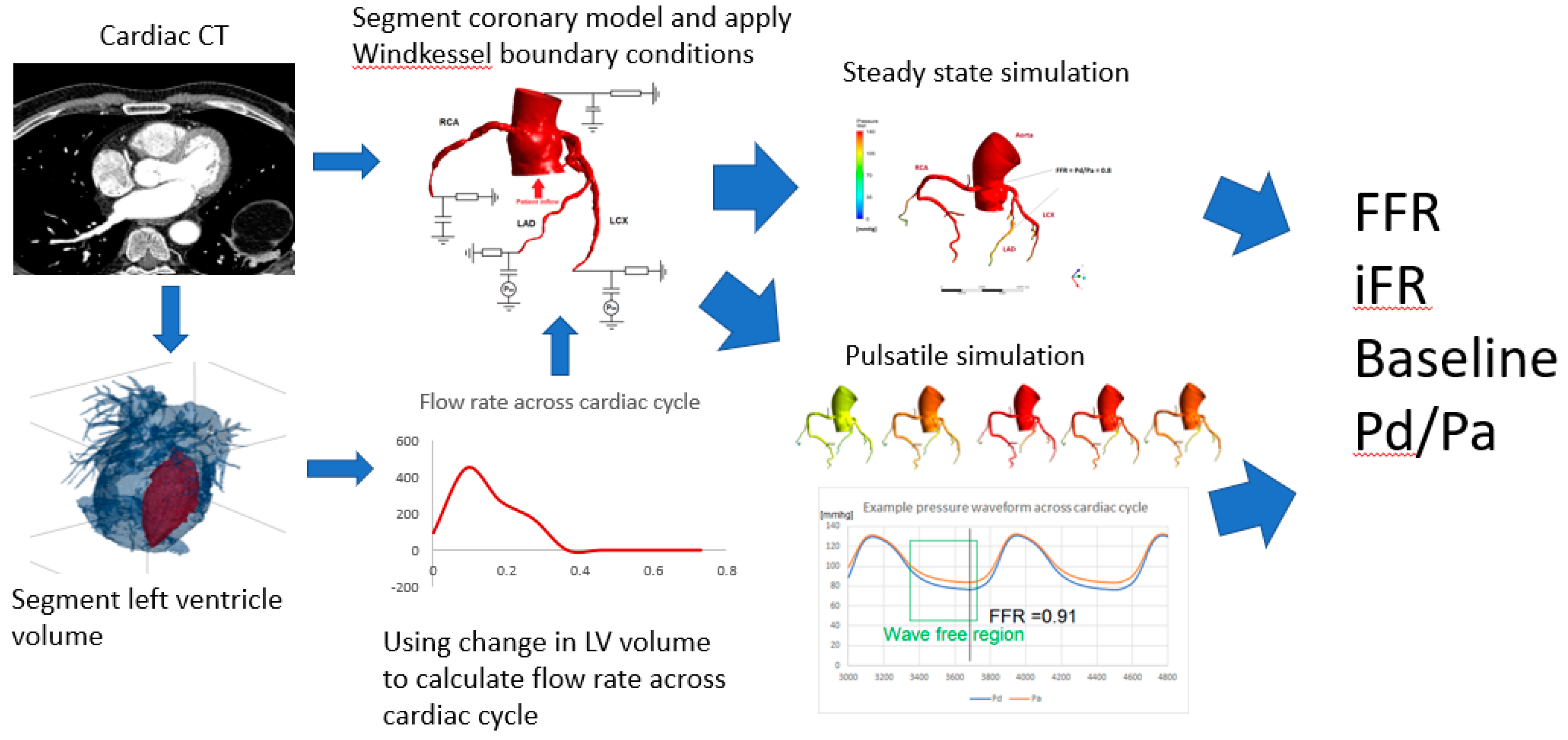
Our analyses were computational fluid dynamics applied to a 3D patient-specific anatomical model, following the steps summarized in Figure 1. To investigate the dependency of FFR values on boundary conditions, we varied the inflow conditions in 4 ways: (1) pulsatile patient-specific, (2) steady inflow patient-specific, (3) pulsatile population average and (4) steady inflow population average. Additionally, the same conditions were also applied to calculate FFR alternatives such as iFR and baseline Pd/Pa. Details of the procedure in each stage of the analysis were described in the following sections.
2.1. Patients
We selected 4 patients (2 males, 2 females, age: 58 + 6 years) of various levels of angiographically determined epicardial stenosis (2 mild, 1 moderate and 1 severe case). The patients presented chest pain and other symptoms that indicated an intermediate risk of coronary artery disease. All patients underwent cardiac CT angiography for anatomical assessment. The study was carried out in accordance with the recommendations of the South East Research Ethics Research Committee, Aylesford, Kent, UK, with written informed consent from all subjects. All subjects gave written informed consent in accordance with the Declaration of Helsinki.
2.2. Image Segmentation and Meshing
Three-dimensional anatomical models of the coronary arteries were obtained by segmenting the coronary CT angiography images using the Simpleware ScanIP package (Synopsys, Mountain View, CA, USA). Due to the limiting resolution of CT, approximately 0.488 mm per pixel in-plane and 0.625 mm slice thickness, the anatomical model included arteries whose diameter was larger than 2 mm. The 3D anatomical model was meshed using tetrahedral elements with 6 layers of prism elements near the wall. Total number of elements resulted in the order of 106 for all patients.
2.3. Computational Model of Blood Flow
The blood flow in the anatomical models was computed by numerically solving the incompressible 3D Navier–Stokes equations below, using a commercial package ANSYS CFX 17.0 (ANSYS, Inc., Cannonsburg, MI, USA).
Here, is velocity vector, is pressure and and are density and viscosity of the blood, respectively. Blood was assumed to be homogenous and a Newtonian fluid, with its density and dynamic viscosity being 1060 kg/m3 and 0.004 Pa s, respectively. Although the blood is a non-Newtonian fluid, it was assumed to be Newtonian, i.e., with a constant viscosity, considering the shear-thinning nature of the blood with almost constant apparent viscosity for shear rate over 100 s−1 that is typically seen in the coronary arteries [23,24]. Because the Reynolds number is below 1000 in the coronary arteries even considering an extremely high velocity of 1.0 m/s with 3.0 mm vessel diameter, density and viscosity of the blood as above, the flow was assumed to be laminar. The vessel wall was approximated as rigid wall, where non-slip boundary conditions were applied, and cardiac-induced wall motion was not incorporated.
2.4. Patient Specific Inflow Boundary Conditions
Retrospectively gated CT was performed/acquired, with the data binned into 10% R–R intervals, to enable segmentation of the LV cavity. Using these CT snapshots, the left ventricular cavity was segmented. By calculating the change in volume across each time point, the aortic outflow, which subsequently splits into the systemic and coronary outflow, was calculated as a function of time (Figure 2). Here, the flow was assumed to be zero in the diastolic phase of the cardiac cycle after the LV cavity volume started to increase.
For the steady-state simulation, the patient-specific stroke volume was calculated from the difference between the end-diastolic and end-systolic volumes, and combined with the measured heart rate of the patient to obtain their time-averaged flow rate. For the pulsatile flow simulation, the patient-specific flow waveform was used directly as an inflow condition at the aortic inlet.
2.5. Two-Element Windkessel Model for Outlet Boundaries
The two-element or RC Windkessel model is a 0D hydraulic–electric analogue where vascular resistance and vessel compliance are represented analogous to electrical resistance and capacitance [25,26]. Similarly, flow properties like a pressure difference and mass flow is analogous to a potential difference and electrical current. The downstream boundary condition after the RC component is essentially the venous bed approximated to have zero pressure.
There have been many Windkessel models developed, e.g., the three-element, four-element modified Windkessel and others [26,27,28]; however, complex models require more parameter estimation for each individual component in the circuit. We chose to use two-element model for simplicity. The limitation of the two-element Windkessel model is its inability to accurately replicate the high frequency component in the pressure waveform during systole, because it is essentially a low-pass filter. However, for the purpose of estimating the behavior in the diastolic wave-free region, it performs similar to more complex models [26].
There are two parameters that need to be determined: vessel downstream resistance and compliance. The methods of calculating these will be outlined below for the various outlet boundaries in the model.
2.6. Aortic Outflow Boundary Condition
The aortic outflow is a single boundary located just prior to the aortic arch and accounts for the cardiac output to the rest of the body. Here, it is a simple two-element Windkessel model with systemic resistance tuned to account for 95% of the cardiac output when compared to the resistance values of the coronary outputs. The compliance values were chosen to produce realistic pressure waveforms at the outlet based on literature data [20]. The total resistance of all the outlets—systemic and coronary—was scaled to the patient-specific or population systolic and a diastolic pressure.
2.7. Coronary Outflow Boundary Condition
The coronary arteries in the anatomical model were terminated at approximately 2 mm vessel diameter, as it approached the limitations of the CT resolution. To incorporate the resistance of further downstream geometry, a structured tree model proposed by Olufsen [29] was used. In this method, the vascular network after the terminal boundary was modelled with a tree of asymmetric fractal-like bifurcations where each daughter branch of a bifurcation further divided into asymmetric branches recursively. The method was based on empirical studies on geometry of the coronary microvasculature and had been shown to produce realistic resistance conditions for coronary flow simulations [30].
This process was terminated when the smallest of the daughter branches reached a size that was the limiting size for arterioles—this was 0.05 mm in our model following Olufsen et al. [29]. The resistance of entire tree was calculated and represented the resistance component of two-element Windkessel model, as shown in Figure 3. Note that as the simulation is for FFR, they need to be adjusted for adenosine-induced hyperaemia, which is explained in the next section. The capacitance parameter was determined by setting the time constant (=1/RC) equal to 0.063 s following the literature [20].
2.8. Modelling the Effect of Adenosine
Adenosine induces direct coronary arteriolar vasodilation through specific activation of the A2A receptor. This usually results in a 3.5- to 4-fold increase in myocardial blood flow. Under such hyperaemic conditions, coronary blood flow is directly proportional to perfusion pressure and a reduction in perfusion pressure due to a coronary stenosis will thus proportionally decrease coronary flow during hyperaemia.
In some extreme cases of disease, it is possible for the absolute flow to be lower than that at the resting state; this is known as Coronary Steal [31]. To mimic the effect of vasodilation on our model, the resistance values (obtained using the structured tree method) in our Windkessel boundary condition is uniformly decreased to 30% of the resistance at rest; this is a typical adenosine response and used in previous coronary simulations [20]. Here, the increase of the flow by adenosine administration from the baseline state (Qadenosine/Qbaseline) is called coronary flow reserve (CFR), indicating the ability of vasodilation in a branch and its downstream vasculature.
Adenosine has also been found to increase the heart rate by 40–50% of baseline [32,33] as well as stroke volume to a much lesser extent (by approximately 10% [32]), ultimately increasing the average cardiac output. The patients in this study had their heart rates and blood pressures measured already during adenosine-induced hyperaemia. Population average haemodynamic parameters (heart rate, etc.) for patients under hyperaemia were adopted from population average baseline cardiac statistics [34,35], and the typical adenosine response was applied as mentioned above [32,33].
2.9. Modelling Intramyocardial Pressure
It is well known that the pressure and flow waveforms in coronary arteries are out of sync, i.e., the flow is not systolic-dominant, which is strongly influenced by the intramyocardial pressure. Intramyocardial pressure is assumed to be purely dependent on and linearly proportional to left ventricular pressure [36,37], and left ventricular pressure closely traces aortic pressure during systole but drops down to nearly zero during diastole. In our model, we applied an intramyocardial pressure on the surrounding pressure across the capacitive component of the Windkessel model boundary condition, as indicated in Figure 3, in the coronary arteries that supply the left ventricle, primarily to the main branches of the left anterior descending artery (LAD) and left circumflex artery (LCx). We adopted the intramyocardial pressure waveform from the literature, which was scaled to patient-specific systolic pressure, while the diastolic pressure was kept zero [38].
2.10. Computational Schemes and Parameters
In ANSYS CFX, the governing equations were discretised in space using element-based finite volume method, where volume and surface integrations were performed at the Gaussian integration points on each element/face using tri-linear shape function, interpolating nodal values of velocity and pressure in 3D within each element. The time integration was performed using 2nd order backward Euler scheme. Stabilization of the advection term was achieved by adaptive 2nd order upwinding scheme, in which 1st order upwinding was blended with the 2nd order scheme such that the nodal value of any variable did not exceed the maximum/minimum bounds of surrounding nodal values. For more details, readers are referred to CFX theory manual [39].
The time step for pulsatile/transient simulations used was 0.001 s, and the convergence criteria for the linear iterative solver was set to 1.0 × 10⁻⁵ based on the root-mean-square of the residual at every node. Pulsatile simulations required 3 cycles before it stabilised to a consistent waveform, and therefore all simulations were performed up to 5 cycles. The actual time of simulation and total number of time steps varied between patients, as their heart rate determined the length of the simulation. The steady inflow simulations were carried out in quasi-steady condition, i.e., transient simulations were conducted with the steady inflow boundary condition. This was required to account for the transient response of the downstream impedance. Here, the same time steps (0.001 s) and convergence criteria (1.0 × 10⁻⁵) as the fully-transient simulations were used. Sensitivity tests of the computational results to both mesh and time step size were carried out such that the pressure drop across a stenosis computed with the finally-chosen mesh and time step was less than 1% of difference compared to a mesh with doubled number of elements. Computations were conducted using 2 cores on standard desktop workstations (Intel Core i7 6700K 4 GHz, 16 GB RAM, 4 cores and Intel Xeon E5-2670 2.6 GHz, 128 GB RAM, 32 cores).
2.11. Calculation of FFR and Other Metrics
Monitor points were placed at the coronary ostium and in the coronary artery at a point approximately 4 cm distal to the stenosis. FFR standards in invasive measurements specify at least 2–3 cm distally [40]. In the steady inflow simulation, the pressure ratio of the two points when the simulation had stabilized and converged was used to represent FFR. In the pulsatile flow simulation, pressure values at each monitor point were recorded across the cardiac cycles to calculate FFR (Figure 4). FFR was taken as the lowest value measured (i.e., the most severe measure) following common clinical practice. FFR of less than 0.8 is deemed as a physiologically significant stenosis that should be best treated by stenting.
The instantaneous wave-free ratio or iFR was similar to the pressure ratio across the stenosis; however, it was measured during rest (no induced hyperaemia) and it was the average value across the “wave-free” region of the cardiac cycle, where the competing forces of aortic compression and microvascular compression were minimal and where pressure and flow became linearly related. In this region, vessel resistance was at a minimum and stable throughout. The cutoff threshold of iFR indicating significant stenosis was <0.89 [11].
2.12. Comparison of Patient-Specific Parameters and Population Average-Based Inflow Parameters
Simplification of models by using population average data for boundary conditions is a widely-accepted approach. While that may not reduce the simulation time required to produce FFR values, it reduces the burden on clinicians to record every patient-specific parameter for each individual. Adequate level of patient information must be thoroughly investigated by assessing whether the pressure profile and FFR is sensitive to patient specificity in the inflow parameters and in what cases might this cause a significant discrepancy. The population average data under induced hyperaemia [34,35] is listed in Table 1.
3. Results
Typical pressure profiles obtained from the patient-specific CFD simulations, with steady patient-specific inflow and with pulsatile patient-specific inflow, are shown in Figure 5 and Figure 6. The pulsatile simulation result is also accompanied by pressure waveforms in the coronary ostium (Pa) and distal to the stenosis (Pd). Comparison of the two series of the results shows that the pressure profiles are, in general, similar, especially the steady inflow profile and the pulsatile inflow profile at t = 0.2 s appear to be close to each other. In both steady and pulsatile inflow cases, a marked difference in pressure is observed across the stenosis (red-orange-yellow). It is also important to mention that the pressure difference across the stenosis (Pd vs Pa) is nearly constant from the peak flow (~2.5 s) to the end of the cycle in Figure 6. Note that in Figure 4 and Figure 6, the proximal–distal pressure difference is larger in the diastolic period. This is because of the diastolic dominant flow in coronary arteries, shown in Figure 7.
We first examined the impact of the type of inflow boundary conditions—pulsatile, steady, patient-specific and population average—on FFR. Table 2 summarises the result of computations for all four patients and four inflow conditions, in terms of FFR values in various definitions. Note that the conditions of the present study are all hyperemic, which is required for the calculation of FFR. The FFR are, in general, nearly independent of the boundary conditions for Patients 1–3 (approximately 0.6, 0.8, 0.95, respectively) but more variable for Patient 4 (range 0.84–0.94). From the direct comparison between pulsatile and steady conditions for each patient, the maximum discrepancy of FFR due to flow pulsatility is 0.02 for Patient 2. Likewise, the maximum discrepancy of FFR owing to the difference between patient-specific and population-averaged conditions is 0.07 for Patient 4.
Next, we studied the impact of hyperaemic conditions on the flow reserve indicators including iFR—an indicator based on the non-hyperaemic condition. The comparison of various flow reserve indicators is presented in Table 3. Here, all indicators are based on the pressure drop across the stenosis and the difference between those in the baseline and hyperemic conditions are shown. Because FFR by definition requires hyperemia, non-hyperaemic (baseline) pressure drop is shown as Pd/Pa—ratio of the pressure downstream of the stenosis to the aortic pressure. The results were derived with patient-specific flow conditions. The pulsatile FFR was calculated as the average of Pd/Pa throughout the cardiac cycle, whereas iFR was only in the wave-free (diastolic) region. The hyperemic indicators are consistently lower than the baseline ones, and the indicators are in agreement with one another within each category. This is also in agreement with the lower cutoff value of FFR (0.80 [4,6]) in comparison to baseline indicators (e.g., 0.91 for iFR [12]). Among the patients in this study, only Patient 1 appears to be a severe case with a baseline Pd/Pa and iFR below their respective diagnostic cutoffs (0.91 and 0.89). For the same patient, the discrepancy between its baseline Pd/Pa and iFR is also the largest, 0.88 and 0.85. The patients with the higher FFRs also had baseline Pd/Pa and iFR well above the cutoffs, indicating good diagnostic agreement in the two metrics.
Lastly, the distribution of the flows to the stenosed coronary branch and the other non-stenosed branches were investigated under the various inflow boundary conditions. The results are summarised in Table 4. The flow rates through the stenosed branches are closely matched between the two simulation types while the difference in the healthy branch flows tend to be higher. The largest discrepancy in stenosed branch flow rate between pulsatile and steady flow conditions was observed in Patient 3 (2.18 mL/s versus 1.83 mL/s). At the same time, Patient 3 has the highest FFR (i.e., least functionally severe stenosis) and, therefore, it is likely that the pressure drop across the mildly stenosed branch is not affected by the difference of the flow rates.
4. Discussion
4.1. Effect of Flow Pulsatility on FFR
The high correlation between the FFR values obtained using a pulsatile simulation and that of a steady-state simulation indicates that the use of simple steady flow condition may be acceptable. Across the range of coronary artery stenosis from healthy to significantly diseased, the discrepancy of FFR between the steady state and the pulsatile simulation is small (maximum discrepancy of 0.02). This remains true for diseased LAD and LCx arteries, where the systolic–diastolic discrepancy of the flow is particularly high due to its higher impact of intramyocardial pressure that inhibits relatively low level of systolic flow.
The cycle-averaged Pd/Pa ratio from the pulsatile flow simulation is naturally higher than the FFR because of its definition, i.e., FFR is the smallest Pd/Pa throughout the cycle. However, dFFR is not necessarily the smallest FFR, although it tends to approximate closely to FFR. The minimal pressure ratio (=FFR) is almost always found in the wave-free region and usually at the end of diastole, although not always. This is well explained by the fact that the downstream microvascular resistance is stable and minimal in the wave-free region [11], therefore inviting high flow rate that results in a much larger pressure drop in the epicardial stenosis.
The steady-state FFR values are more closely aligned with the standard FFR as opposed to the pulsatile average despite both simulations having the same average flow rate/cardiac output. Referring to the flow distributions (Table 4), the flow in the stenosed branch seems not sensitive to the difference between steady and pulsatile conditions, relative to the non-stenosed branches. This indicates that a stenosis is likely to cause redirections in flow, which make it less sensitive to fluctuations in inflow. This is also consistent with the waveforms presented in Figure 7; the flow in the stenosed branch (LAD) varies less than the healthy branch (LCx).
Additionally, when iFR as well as baseline Pd/Pa in the pulsatile simulation are compared with the steady-state baseline Pd/Pa, the steady-state Pd/Pa tends to be closer in approximating iFR than the cycle-averaged pulsatile baseline Pd/Pa. It is most apparent in the case of Patient 1 where the discrepancy between cycle-averaged pulsatile baseline Pd/Pa and pulsatile iFR is the largest. This suggests that the steady inflow simulations in both resting and hyperaemic states may tend to be more representative of the conditions in the wave-free region of the cardiac cycle. The wave-free region is defined as the time interval within the cardiac cycle where pressure and flow are linearly related [11]. In a steady inflow simulation, the pressure and flows converge to a static value, therefore satisfying this condition.
Steady-state simulations would not be the replacement to pulsatile simulations in all coronary flow simulations; however, there is much value in using them when the focus is on studying the flow limiting effects of a coronary obstruction. It is far simpler to simulate, with less input parameters needed and completed in a much shorter time. The computational time was approximately 2 h for the steady-state simulation, whereas a pulsatile simulation that observes 5 cardiac cycles required approximately 16 h. Using steady-state simulations may vastly improve the efficiency of blood-pressure-focused coronary haemodynamic research and medical diagnostics, especially when a larger population is looked at.
4.2. Importance of Patient Specificity in Inflow Parameters
The largest discrepancy of FFR was observed for Patient 4, approximately 7% larger in the population average simulation than with the patient’s own inflow parameters. The largest disparity between the patient-specific inflow parameters and population-averaged was indeed in Patient 4 (Table 1); the patient-specific cardiac output, heart rate and stroke volume are all universally higher than that of the population average. The lower FFR (i.e., less functionally normal) in Patient 4 is found with patient-specific inflow in both pulsatile and steady-state simulations; therefore, the likely cause of the FFR discrepancy is the cardiac output, not heart rate or stroke volume. Patient 4′s cardiac output is 1.9 times as large as the population average. Using patient-specific inflow, the flow diverted to the stenosed branch is about 1.7 times (5.6 mL/s versus 3.3 mL/s) more than using population average inflow. The discrepancy between the inflow difference (×1.9) and the stenosed branch outflow (×1.7) suggests that the stenosis redirected the increased flow more to healthy branches.
Using the equation for laminar flow resistance: , where Q is flow rate, is pressure drop and R is vascular resistance, a higher flow rate should lead to a proportionately higher pressure drop for the same coronary artery system having the same vascular resistance. With the systolic and diastolic pressures comparable (patient-specific, 128/68 versus population average, 122/71) between patient-specific and the population average conditions for Patient 4, it is reasonable to assume that the pressure drop difference is proportionate to the flow rate difference between the patient-specific and population average inflows (i.e., patient-specific is 1.7 times higher). This is indeed true as the FFR for the patient-specific case indicates a pressure drop of approximately 1.75 times larger than that of population average. However, the definition of FFR (Pd/Pa = (Pa − ∆P)/Pa; ∆P is the pressure drop across the stenosed vessel) reduces the impact of pressure drop, which is why the discrepancy in inflow conditions are not reflected to FFRs. At the same time, the flow in the branches is sensitive to the inflow condition, which indicates that if the focused parameter is not FFR but shear stress, impact of inflow conditions would be more significant.
It has been documented that FFR is related to the relationship between coronary artery lumen volume (V) and left ventricular mass (M). Left ventricular mass is linearly correlated with left ventricular chamber volume (volume/mass ratio 0.80 mL/g + 0.15 mL/g) [42]. Low V/M ratio indicates that a small lumen volume is available for large blood demand (i.e., large volumetric flow) for a large ventricular mass, thus a lower V/M ratio tends towards a lower FFR (high pressure drop) and higher overall likelihood of CAD [43]. It has also been suggested that an obstruction in a small coronary artery lumen volume is likely to cause ischaemia, and more so for a larger LV mass that demands a higher volume of blood [43].
4.3. Various Definitions of Flow Reserve Parameters
The various metrics alternative to FFR—for gauging physiological severity of an obstruction—fundamentally evaluate the pressure ratio Pd/Pa in various definitions, each of which has its own merits. The main advantage of iFR, or baseline/resting Pd/Pa, lies in its measurement procedure, i.e., the intravascular pressure measurement is free from adenosine. From a simulation perspective, it may seem irrelevant; however, setting microvascular resistance and appropriately determining its response to vasodilatory drugs as the coronary outlet conditions is crucially important, although acquisition of such data in patient-specific manner is a challenge. It has been reported that coronary artery haemodynamic simulations are particularly sensitive to their outlet conditions [14,21]. While a typical adenosine response is often used, e.g., reduction of peripheral resistance to 30% of baseline, the response in reality is highly variable and more importantly, diseased patients’ vasodilatory response is typically less than optimal. Therefore, using an adenosine/vasodilator-free method even in simulation provides a substantial advantage by potentially mitigating the unknown.
Among the patients, Patient 2 is a borderline case according to the FFR; both pulsatile and steady-state simulations gave a value of 0.80–0.81, which is right at the cutoff for stenting treatment. On the other hand, the baseline Pd/Pa for both pulsatile and steady-state simulation (0.92 and 0.94) indicate that they are both above the optimal cutoff of 0.91 [11] for determining a significant stenosis. Similarly, the iFR obtained from measuring the Pd/Pa ratio at the wave-free region (0.93) indicates that the stenosis is not severely flow limiting, using the iFR cutoff of 0.89. Adenosine-free methods such as iFR and baseline Pd/Pa is not only beneficial for invasive assessment but also for simulation-based assessment of coronary artery disease. As mentioned in the introduction, a hybrid approach using multiple flow reserve parameters (e.g., FFR and iFR) has been considered. The results demonstrate that computationally-derived flow reserve parameters could provide a more consolidated indication when one parameter shows a borderline result.
4.4. Limitations and Future Work
This investigation is a pilot study with a small sample size, including mild to severe range of coronary artery disease. The inflow waveform was taken from a series of chest 4D CTs across the cardiac cycle divided into 10 equal intervals. A more in-depth examination of the pulsatile effects especially around the systolic peak will require waveforms with more sampling points over the cycle, which may be acquired with 4D CT of a much higher temporal resolution, time-resolved MRI or invasive flow measurements. However, as FFR and iFR tend to be measured during diastole in the wave-free region, an increased complexity in simulating the systolic region may not provide any additional benefit.
We focused on CT-based calculation of FFR in this paper, but other approaches exist. For example, quantitative flow ratio (QFR), an FFR-equivalent parameter was calculated based on the 3D model reconstructed from 2 projections of X-ray angiograms [44]. Such approaches have their own advantages and disadvantages, but the discussion of that is out of the scope of our paper.
Although the trend of flow reserve parameters we observed in this study—they are not strongly sensitive to the inflow boundary conditions—appears consistent, this research can be furthered in two major directions: (1) using a larger sample size comparing the various inflow boundary conditions, and (2) verifying the result with the gold standard, i.e., invasively measured FFR. There are other factors, such as outflow boundary conditions, that potentially affect FFR, and future studies to examine those factors are also warranted.
Author Contributions
Conceptualization, R.T. and L.J.M.; methodology, E.W.C.L. and R.T.; formal analysis, E.W.C.L. and R.T.; investigation, E.W.C.L., L.J.M. and R.T.; resources, R.T.; data curation, L.J.M.; writing—original draft preparation, E.W.C.L.; writing—review and editing, E.W.C.L., L.J.M. and R.T.; visualization, E.W.C.L.; supervision, R.T. and L.J.M.; funding acquisition, L.J.M. and R.T.
Funding
This work was supported by the EPSRC-funded UCL Centre for Doctoral Training in Medical Imaging (EP/L016478/1) and the Department of Health’s NIHR-funded Biomedical Research Centre at University College London Hospitals.
Acknowledgments
The authors acknowledge Raymond Endozo (Nuclear Medicine, UCL Hospital) for his help on data collection.
Conflicts of Interest
The authors declare there is no conflict of interest.
References
- Townsend, N.; Williams, J.; Bhatnagar, P.; Wickramasinghe, K.; Rayner, M. Cardiovascular Disease Statistics 2014; British Heart Found: London, UK, 2014. [Google Scholar]
- Montalescot, G.; Sechtem, U. 2013 ESC guidelines on the management of stable coronary artery disease—Addenda. Eur. Heart J. 2013, 34, 2949–3003. [Google Scholar] [CrossRef] [PubMed]
- Hachamovitch, R.; Hayes, S.W. Comparison of the short-term survival benefit associated with revascularization compared with medical therapy in patients with no prior coronary artery disease undergoing stress myocardial perfusion single photon emission computed tomography. Circulation 2013, 107, 2900–2906. [Google Scholar] [CrossRef] [PubMed]
- Tonino, P.A.; Fearon, W.F. Angiographic Versus Functional Severity of Coronary Artery Stenosis in the FAME Study. Fractional Flow Reserve Versus Angiography in Multivessel Evaluation. J. Am. Coll. Cardiol. 2010, 55, 2816–2821. [Google Scholar] [CrossRef] [PubMed]
- De Bruyne, B.; Sarma, J. Fractional flow reserve: A review. Heart 2008, 94, 949–959. [Google Scholar] [CrossRef] [PubMed]
- Heyndrickx, G.R.; Toth, G.G. The FAME Trials: Impact on Clinical Decision Making. Int. Cardiol. Rev. 2016, 11, 116–119. [Google Scholar] [CrossRef] [Green Version]
- De Bruyne, B.; Pijls, N. Fractional flow reserve guided PCI versus medical therapy in stable coronary disease. N. Engl. J. Med. 2012, 367, 991–1001. [Google Scholar] [CrossRef]
- Achenbach, S.; Rudolph, T. Performing and Interpreting Fractional Flow Reserve Measurements in Clinical Practice: An Expert Consensus Document. Interv. Cardiol. 2017, 12, 97–109. [Google Scholar] [CrossRef] [Green Version]
- Abe, M.; Tomiyama, H. Diastolic fractional flow reserve to assess the functional severity of moderate coronary artery stenoses: Comparison with fractional flow reserve and coronary flow velocity reserve. Circulation 2000, 102, 2365–2370. [Google Scholar] [CrossRef]
- Chalyan, D.A.; Zhang, Z. End-Diastolic Fractional Flow Reserve. Circul. Cardiovasc. Interv. 2014, 7, 28–34. [Google Scholar] [CrossRef] [Green Version]
- Sen, S.; Escaned, J. Development and Validation of a New Adenosine-Independent Index of Stenosis Severity from Coronary Wave–Intensity Analysis: Results of the ADVISE (ADenosine Vasodilator Independent Stenosis Evaluation) Study. J. Am. Coll. Cardiol. 2012, 59, 1392–1402. [Google Scholar] [CrossRef]
- Escaned, J.; Ryan, N. Safety of the Deferral of Coronary Revascularization on the Basis of Instantaneous Wave-Free Ratio and Fractional Flow Reserve Measurements in Stable Coronary Artery Disease and Acute Coronary Syndromes. JACC Cardiovasc. Interv. 2018, 11, 1437–1449. [Google Scholar] [CrossRef] [PubMed]
- Gaur, S.; Achenbach, S. Rationale and design of the HeartFlowNXT (HeartFlow analysis of coronary blood flow using CT angiography: NeXt sTeps) study. J. Cardiovasc. Comput. Tomogr. 2013, 7, 279–288. [Google Scholar] [CrossRef] [PubMed]
- Morris, P.D.; van de Vosse, P. “Virtual” (Computed) Fractional Flow Reserve. JACC Cardiovasc. Interv. 2015, 8, 1009–1017. [Google Scholar] [CrossRef] [Green Version]
- Norgaard, B.L.; Leipsic, J. Diagnostic performance of noninvasive fractional flow reserve derived from coronary computed tomography angiography in suspected coronary artery disease: The NXT trial (Analysis of Coronary Blood Flow Using CT Angiography: Next Steps). J. Am. Coll. Cardiol. 2014, 63, 1145–1155. [Google Scholar] [CrossRef] [PubMed]
- Faster. On-Site FFRCT May Be on the Horizon Through Innovation and Collaboration. Available online: https://www.tctmd.com/news/faster-site-ffrct-may-be-horizon-through-innovation-and-collaboration (accessed on 20 November 2018).
- Boileau, E.; Pant, S. Estimating the accuracy of a reduced-order model for the calculation of fractional flow reserve (FFR). Int. J. Numer. Methods Biomed. Eng. 2018, 34, e2908. [Google Scholar] [CrossRef] [PubMed]
- HeartFlowNXT—HeartFlow Analysis of Coronary Blood Flow Using Coronary CT Angiography (HFNXT). Available online: https://clinicaltrials.gov/ct2/show/NCT01757678 (accessed on 20 November 2018).
- Trial Demonstrates HeartFlow FFRCT Analysis Significantly Lowers Cost of Care, Improves Quality of Life for Coronary Artery Disease. Available online: https://hfdc-corpweb.s3-us-west-2.amazonaws.com/assets/docs/TCT-PLATFORM-Press-Release/TCT-PLATFORM-Press-Release.html (accessed on 20 November 2018).
- Kim, H.; Vignon-Clementel, I. Patient-specific modeling of blood flow and pressure in human coronary arteries. Ann. Biomed. Eng. 2010, 39, 3195–3209. [Google Scholar] [CrossRef] [PubMed]
- Siogkas, P.; Papafaklis, A. Patient-Specific Simulation of Coronary Artery Pressure Measurements: An In Vivo Three-Dimensional Validation Study in Humans. BioMed Res. Int. 2015, 2015, 628416. [Google Scholar] [CrossRef]
- Morris, P.D.; Soto, D.A.S. Fast Virtual Fractional Flow Reserve Based Upon Steady-State Computational Fluid Dynamics Analysis: Results From the VIRTU-Fast Study. JACC Basic Transl. Sci. 2017, 2, 434–446. [Google Scholar] [CrossRef]
- Hanson, S.R.; Sakariassen, K.S. Blood flow and antithrombotic drug effects. Am. Heart J. 1998, 135, 132–145. [Google Scholar] [CrossRef]
- Tenekecioglu, E.; Torii, R. Difference in haemodynamic microenvironment in vessels scaffolded with Absorb BVS and Mirage BRMS: Insights from a preclinical endothelial shear stress study. EuroIntervention 2017, 13, 1327–1335. [Google Scholar] [CrossRef]
- Sagawa, K.; Lie, R.K. Translation of Otto frank’s paper “Die Grundform des arteriellen Pulses” zeitschrift für biologie 37: 483–526 (1899). J. Mol. Cell. Cardiol. 1990, 22, 253–254. [Google Scholar] [CrossRef]
- Westerhof, N.; Lankhaar, J. The arterial windkessel. Med. Biol. Eng. Comput. 2009, 47, 131–141. [Google Scholar] [CrossRef] [PubMed]
- Mantero, S.; Pietrabissa, R. The coronary bed and its role in the cardiovascular system: A review and an introductory single-branch model. J. Biomed. Eng. 1992, 14, 109–116. [Google Scholar] [CrossRef]
- Francis, S.E. Continuous Estimation of Cardiac Output and Arterial Resistance from Arterial Blood Pressure Using a Third-Order Windkessel Model. Master’s Thesis, Massachusetts Institute of Technology, Department of Electrical Engineering and Computer Science, Cambridge, MA, USA, 2007. [Google Scholar]
- Olufsen, M.S. Structured tree outflow condition for blood flow in larger systemic arteries. Am. J. Physiol.-Heart Circ. Physiol. 1999, 276, H257–H268. [Google Scholar] [CrossRef]
- Olufsen, M.S.; Peskin, C.S. Numerical simulation and experimental validation of blood flow in arteries with structured-tree outflow conditions. Ann. Biomed. Eng. 2000, 28, 1281–1299. [Google Scholar] [CrossRef] [PubMed]
- Gould, K.L. Coronary steal. Is it clinically important? Chest 1989, 96, 227–228. [Google Scholar] [CrossRef] [PubMed]
- Reyes, E.; Loong, C.Y. High-Dose Adenosine Overcomes the Attenuation of Myocardial Perfusion Reserve Caused by Caffeine. J. Am. Coll. Cardiol. 2008, 52, 2008–2016. [Google Scholar] [CrossRef] [PubMed] [Green Version]
- Morgan, J.M.; McCormack, D.G. Adenosine Vasodilator in Primary Pulmonary Hypertension. Circulation 1991, 84, 1145–1149. [Google Scholar] [CrossRef] [PubMed]
- NCD Risk Factor Collaboration (NCD-RisC). Worldwide trends in blood pressure from 1975 to 2015: A pooled analysis of 1479 population-based measurement studies with 19.1 million participants. Lancet 2017, 389, 37–55. [Google Scholar] [CrossRef]
- Wright, J.D.; Hughes, J.P. Mean Systolic and Diastolic Blood Pressure in Adults Aged 18 and Over in the United States, 2001–2008. Natl. Health Stat. Rep. 2011, 35, 1–22, 24. [Google Scholar]
- Bovendeerd, P.H.M.; Borsje, T. Artsetal. Dependence of intramyocardial pressure and coronary flow on ventricular loading and contractility: A model study. Ann. Biomed. Eng. 2016, 34, 1833–1845. [Google Scholar] [CrossRef] [PubMed]
- Sun, Y.; Gewirtz, H. Estimation of intramyocardial pressure and coronary blood flow distribution. Am. J. Physiol.-Heart Circ. Physiol. 1988, 255, H664–H674. [Google Scholar] [CrossRef] [PubMed]
- Salisbury, P.F.; Cross, C.E. Intramyocardial pressure and strength of left ventricular contraction. Circ. Res. 1962, 10, 608–623. [Google Scholar] [CrossRef] [PubMed]
- CFX Solver Theory Manual; ANSYS: Canonsburg, PA, USA, 2006.
- Solecki, M.; Kruk, M. What is the optimal anatomic location for coronary artery pressure measurement at CT-derived FFR? J. Cardiovasc. Comput. Tomogr. 2017, 11, 397–403. [Google Scholar] [CrossRef] [PubMed]
- Sen, S.; Petraco, R. Wave intensity analysis in the human coronary circulation in health and disease. Curr. Cardiol. Rev. 2014, 10, 17–23. [Google Scholar] [CrossRef]
- Byrd, B.F.; Wahr, D. Left Ventricular Mass and Volume/Mass Ratio Determined by Two-Dimensional Echocardiography in Normal Adults. J. Am. Coll. Cardiol. 1985, 6, 1021–1025. [Google Scholar] [CrossRef]
- Taylor, C.A.; Gaur, S. Effect of the ratio of coronary arterial lumen volume to left ventricle myocardial mass derived from coronary CT angiography on fractional flow reserve. J. Cardiovasc. Comput. Tomogr. 2017, 11, 429–436. [Google Scholar] [CrossRef] [PubMed]
- Tu, S.; Westra, J.; Yang, J.; von Birgelen, C.; Ferrara, A.; Pellicano, M.; Nef, H.; Tebaldi, M.; Murasato, Y.; Lansky, A.; et al. Diagnostic Accuracy of Fast Computational Approaches to Derive Fractional Flow Reserve from Diagnostic Coronary Angiography: The International Multicenter FAVOR Pilot Study. JACC Cardiovasc. Interv. 2016, 9, 2024–2035. [Google Scholar] [CrossRef]
Figure 1.
Flow chart of computational procedure.

Figure 2.
Red line indicates the aortic flow rate across the cardiac cycle, derived from the changing volume of the left ventricular cavity contracting and relaxing across the cardiac cycle, shown by the green line.
Figure 2.
Red line indicates the aortic flow rate across the cardiac cycle, derived from the changing volume of the left ventricular cavity contracting and relaxing across the cardiac cycle, shown by the green line.

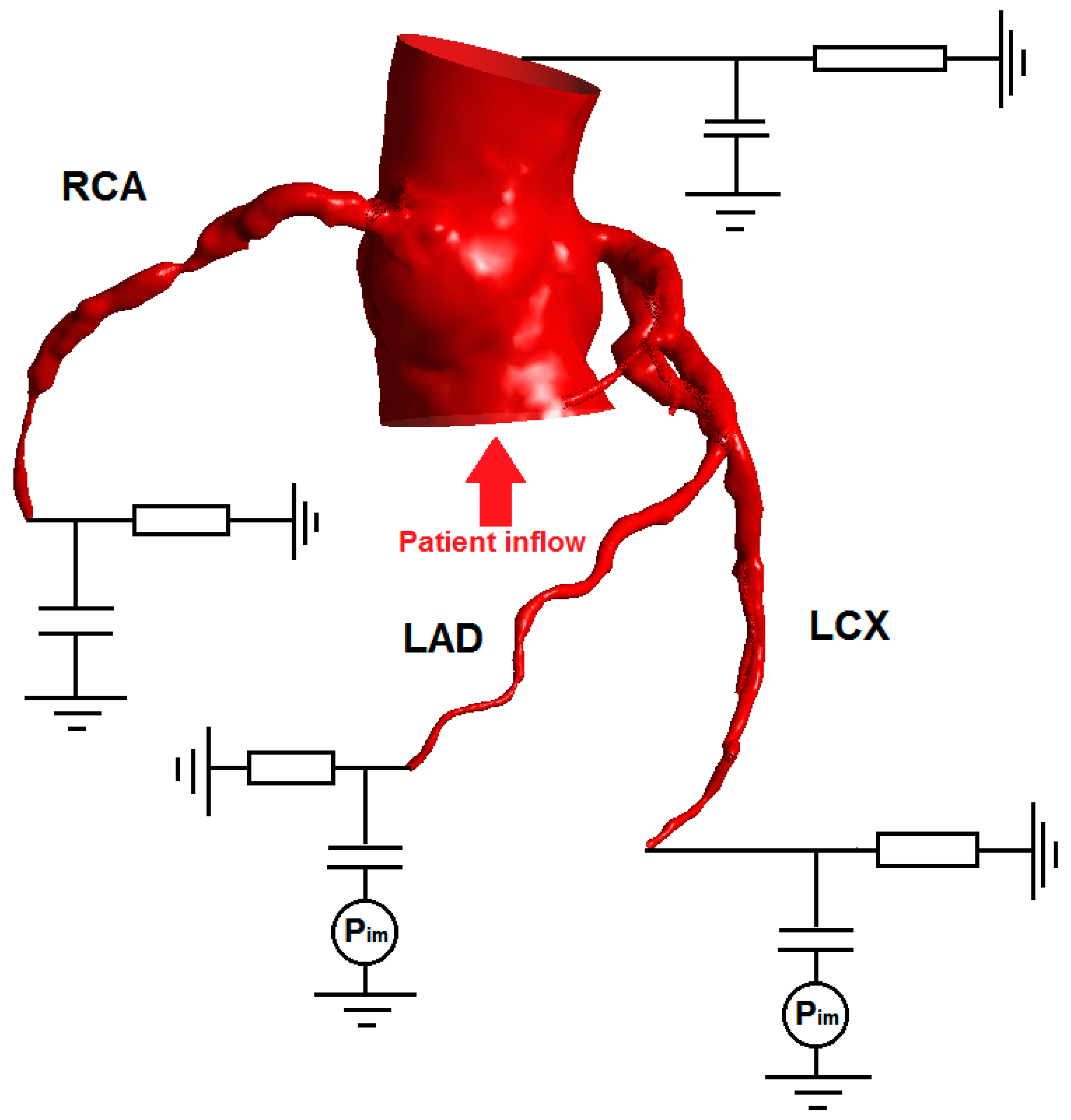
Figure 3.
Schematic showing various outlet boundary conditions. All the boundary conditions are two-element Windkessel models represented in the circuit diagram. In this patient, both the left anterior descending artery (LAD) and left circumflex artery (LCx) supply the left ventricle, which is susceptible to higher levels of intramyocardial pressure. Thus a pressure term is applied to the boundary condition for LAD and LCx, to mimic the contraction of the left ventricle causing the embedded coronary arteries to be compressed and reduced flow. However, the intramyocardial pressure was not included in the right coronary artery (RCA) outlet boundary condition.

Figure 4.
Pressure waveform of a patient under induced hyperaemia, showing the pressure at the coronary ostium (Pa) and pressure distal to an obstruction (Pd) across the cardiac cycle. Fractional flow reserve (FFR) is measured as the lowest ratio Pd/Pa measured. Note that there is a region in diastole known as the wave- free region, where the gradient of both pressure and flow are aligned and peripheral resistance is minimized. This is when the pressure drop is usually the most prominent across an obstruction. Instantaneous wave-free ratio (iFR) is measured in that region if the patient is at rest.

Figure 5.
Pressure profile of patient with an obstruction in the LAD. At 0.8 FFR, this patient is in the borderline area where stenting is only marginally better than optimal medical therapy. This pressure profile is obtained from the steady inflow simulation.
Figure 5.
Pressure profile of patient with an obstruction in the LAD. At 0.8 FFR, this patient is in the borderline area where stenting is only marginally better than optimal medical therapy. This pressure profile is obtained from the steady inflow simulation.

Figure 6.
Pressure profile of the same patient as Figure 5 for a pulsatile flow simulation. The stenosis is located on the LAD. In the time history of pressure, result from the last 3 cycles are shown.
Figure 6.
Pressure profile of the same patient as Figure 5 for a pulsatile flow simulation. The stenosis is located on the LAD. In the time history of pressure, result from the last 3 cycles are shown.

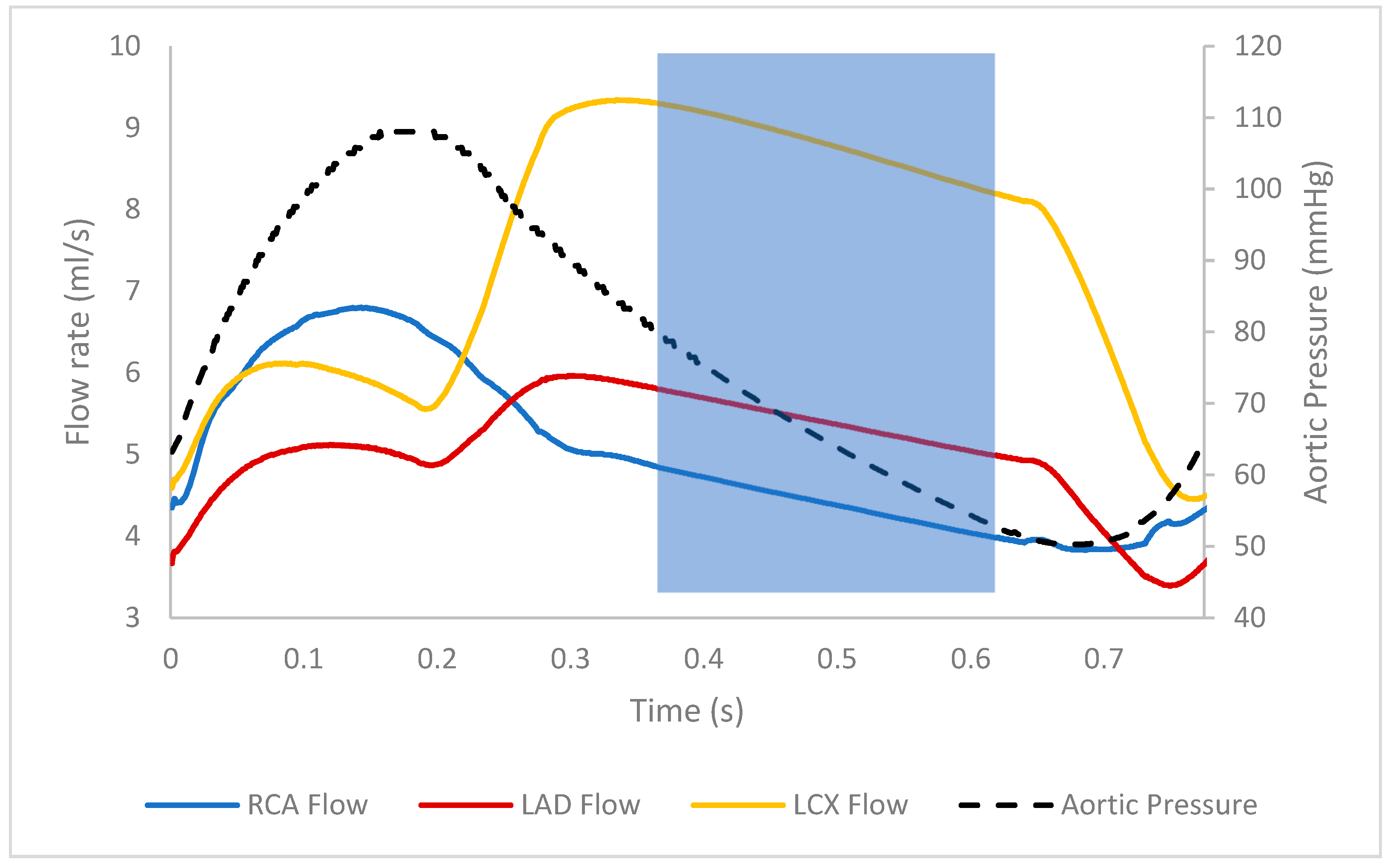
Figure 7.
Flow rates of the various coronary branches across the cardiac cycle. In the left coronary arteries, flow is the highest during diastole due to high intramyocardial pressure during systole inhibiting flow. Note that there is a stenosis in LAD of this patient. The highlighted region shows the diastolic wave-free region, where flow and pressure decline together [11,41].


Table 1.
Patient-specific and population average inflow parameters during hyperaemia. Note: the heart rate is elevated due to adenosine administration.
Table 1.
Patient-specific and population average inflow parameters during hyperaemia. Note: the heart rate is elevated due to adenosine administration.
| Patient | Heart Rate (bpm) | Pressure (mmHg) | Stroke Volume (mL) | Cardiac Output (mL/min) |
|---|---|---|---|---|
| 1 | 106 | 114/68 | 98 | 7200 |
| 2 | 79 | 140/58 | 114 | 9000 |
| 3 | 99 | 108/46 | 68 | 6800 |
| 4 | 115 | 128/68 | 124 | 14,300 |
| Population average [35,36] | 98 | 122/71 | 77 | 7500 |
Table 2.
Comparison of pressure ratio/FFR values obtained using various types of simulation.
| Patient | With Patient-Specific Inflow | With Population Average Inflow | ||||||
|---|---|---|---|---|---|---|---|---|
| Pulsatile Average Pd/Pa | Puls. End-Diastole (dFFR) | Puls. Min (FFR) | Steady State (FFR) | Puls. Average Pd/Pa | Puls. End-Diastole (dFFR) | Puls. Min (FFR) | Steady State (FFR) | |
| 1 | 0.63 | 0.59 | 0.59 | 0.60 | 0.62 | 0.59 | 0.59 | 0.59 |
| 2 | 0.84 | 0.81 | 0.80 | 0.80 | 0.85 | 0.81 | 0.80 | 0.81 |
| 3 | 0.96 | 0.94 | 0.94 | 0.95 | 0.97 | 0.96 | 0.95 | 0.96 |
| 4 | 0.88 | 0.84 | 0.84 | 0.86 | 0.94 | 0.91 | 0.91 | 0.92 |
Table 3.
Comparison of pulsatile FFR, iFR, resting Pd/Pa, steady-state FFR and resting Pd/Pa. Simulations were done using patient-specific inflows.
Table 3.
Comparison of pulsatile FFR, iFR, resting Pd/Pa, steady-state FFR and resting Pd/Pa. Simulations were done using patient-specific inflows.
| Patient | Hyperamic Indicators | Baseline Indicators | |||
|---|---|---|---|---|---|
| Pulsatile FFR | Steady-State FFR | Pulsatile iFR | Pulsatile Baseline Pd/Pa | Steady-State Baseline Pd/Pa | |
| 1 | 0.59 | 0.60 | 0.85 | 0.88 | 0.85 |
| 2 | 0.80 | 0.80 | 0.93 | 0.94 | 0.92 |
| 3 | 0.94 | 0.95 | 0.98 | 0.99 | 0.98 |
| 4 | 0.84 | 0.86 | 0.95 | 0.96 | 0.95 |
Table 4.
Comparison of flow rates out of stenosed and healthy branches, pulsatile versus steady. Simulations were done using patient-specific inflows.
Table 4.
Comparison of flow rates out of stenosed and healthy branches, pulsatile versus steady. Simulations were done using patient-specific inflows.
| Patient | Stenosed Branch Flow Rate | Healthy Branch Flow Rate 1 | ||
|---|---|---|---|---|
| Pulsatile Inflow 2 (mL/s) | Steady Inflow (mL/s) | Pulsatile Inflow 2 (mL/s) | Steady Inflow (mL/s) | |
| 1 | 4.44 | 4.28 | 14.3 | 11.6 |
| 2 | 1.18 | 1.15 | 14.6 | 11.0 |
| 3 | 2.18 | 1.83 | 11.6 | 9.10 |
| 4 | 5.74 | 5.59 | 20.8 | 18.6 |
1 Sum of flow out of branches that are not diseased; 2 instantaneous flow rates measured at the time point of FFR measurement.
© 2019 by the authors. Licensee MDPI, Basel, Switzerland. This article is an open access article distributed under the terms and conditions of the Creative Commons Attribution (CC BY) license (http://creativecommons.org/licenses/by/4.0/).
Share and Cite
MDPI and ACS Style
Lo, E.W.C.; Menezes, L.J.; Torii, R. Impact of Inflow Boundary Conditions on the Calculation of CT-Based FFR. Fluids 2019, 4, 60. https://doi.org/10.3390/fluids4020060
AMA Style
Lo EWC, Menezes LJ, Torii R. Impact of Inflow Boundary Conditions on the Calculation of CT-Based FFR. Fluids. 2019; 4(2):60. https://doi.org/10.3390/fluids4020060
Chicago/Turabian StyleLo, Ernest W. C., Leon J. Menezes, and Ryo Torii. 2019. "Impact of Inflow Boundary Conditions on the Calculation of CT-Based FFR" Fluids 4, no. 2: 60. https://doi.org/10.3390/fluids4020060