Article

Does Quantification of Ecosystem Services Depend Upon Scale (Resolution and Extent)? A Case Study Using the InVEST Nutrient Delivery Ratio Model in Georgia, United States

by
Fabio Jose Benez-Secanho
* and
Puneet Dwivedi
Warnell School of Forestry and Natural Resources, University of Georgia, 180 E Green St, Athens, GA 30602, USA
*
Author to whom correspondence should be addressed.
Environments 2019, 6(5), 52; https://doi.org/10.3390/environments6050052
Submission received: 19 April 2019 / Revised: 4 May 2019 / Accepted: 11 May 2019 / Published: 15 May 2019

Abstract

:
Modeling ecosystem services (ESs) intrinsically involves the use of spatial and temporal data. Correct estimates of ecosystem services are inherently dependent upon the scale (resolution and extent) of the input spatial data. Sensitivity of modeling platforms typically used for quantifying ESs to simultaneous changes in the resolution and extent of spatial data is not particularly clear at present. This study used the Nutrient Delivery Ratio (NDR) model embedded in InVEST (Integrated Valuation of Ecosystem Services and Tradeoffs) for ascertaining the sensitivity of the outputs to three digital elevation models (DEM), two land cover datasets, and three precipitation grids for 57 watersheds located in Georgia, United States. Multivariate regression models were developed to verify the influence of the spatial resolution of input data on the NDR model output at two spatial extents (the state of Georgia and six physiographical regions within the state). Discrepancies in nutrient exports up to 77.4% and 168.1% were found among scenarios at the state level for nitrogen and phosphorus, respectively. Land cover datasets differing in resolution were responsible for the highest differences in nutrient exports. Significance (at 5% level) of spatial variables on the model outputs were different for the two spatial extents, demonstrating the influence of scale when modeling nutrient runoff and its importance for better policy prescriptions.

Graphical Abstract

1. Introduction

Ecosystem services (ESs) are defined as the direct and indirect benefits people obtain from ecological systems [1,2]. Although ESs play a critical role in ensuring overall human wellbeing, current estimates suggest that most of them are declining worldwide. For example, Costanza et al. [3] reported that the global loss in ESs due to land use changes was between $4.3 and $20.2 trillion/year from 1997 to 2011. Assigning monetary values to these ESs is important for raising awareness about ESs to decision makers [4,5] and society, at large [6]. Correct valuation of ESs is inherently dependent upon the quantification of ESs [7] which in turn is dependent upon the scale of the input data. Defining the role of scale on the models which are typically used for quantifying ESs is essential for developing an understanding about the possible changes in ESs relative to changes in resolution and extent of the input data. This is especially true, as existing studies use different scales for quantifying ESs [8]. This information could directly feed into policies which focus on maintaining or enhancing ESs over a landscape [9].
The process of quantifying ESs typically integrates spatial and temporal data within a modeling platform resulting in a situation where the outputs are sensitive to the characteristics of the input data [10]. Coarser datasets aggregate information and are more likely to lose heterogeneity and variation [11], causing rare land cover classes with small patch sizes to disappear [12] or altering the terrain’s surface water flow itself [13]. Similarly, substantial differences in the provision of ESs occur when coarser and finer resolution land use datasets are used for quantifying ESs for the same geographical area [12]. Kandziora et al. [14] found that ESs were overestimated in coarser land use maps relative to finer datasets. However, Konarska et al. [15] found a difference of 200% in the monetary values of ESs while comparing outputs obtained using the International Geosphere Biosphere Programme (IGBP) land cover dataset with 1 km spatial resolution with the outputs obtained using National Land Cover Dataset (NLCD) with 30 m spatial resolution. Apart from land cover data, another crucial data for modeling ESs is the digital elevation model (DEM). Although finer spatial data resolution is recommended as the input data in modeling ESs [13], the impact of different DEM resolutions on the model output is not linear and, therefore, unpredictable [16]. For instance, Redhead et al. [17] found that the model output was little affected by DEM and land cover when spatial resolutions less or equal to 100 m were used, but significant effects were found when datasets coarser than 100 m were used.
The complexity of nature is studied using three perspectives particularly in landscape ecology: process, pattern, and scale [18]. The interactions between process and pattern are investigated under a selected scale. Moreover, the scale can be divided into two components of resolution and the extent of the mapped area [8]. A challenge for assigning social, economic, and ecological values to ESs is the inconsistency in methods used for quantifying and mapping ESs across existing studies [19,20]. One major cause of this inconsistency is the use of different spatial data resolution across studies, resulting in outputs which are hard to compare. In addition, studies modeling ESs have a large variation in the spatial extent [8]. In this context, analyzing the effects of simultaneous changes in spatial data resolution and the spatial extent on the outcome of ESs is crucial for better understanding the full effect of scale on the quantification of ESs [9]. This becomes even more important as there is a lack of studies comparing the impact of simultaneous changes in resolution and extent on ESs using similar modeling assumptions for a selected geographical area [21].
Many studies had applied ES models to map and quantify provision of ESs to clarify key areas for conservation and to serve as guidelines for policymakers. For instance, Krueger and Jordan [22] applied the Watershed Management Priority Index (WMPI) to identify conservation priorities aiming to maintain water quality within the Lower Savannah watershed in Georgia, USA, mainly by protecting forests and well-managed agricultural fields. Brown and Quinn [23] used several InVEST (Integrated Valuation of Ecosystem Services and Tradeoffs) models, including the NDR (Nutrient Delivery Ratio) model, to determine the effects of zoning regulations in improving or maintaining provision of ESs in urban watersheds and found that zoning was effective in preventing degradation of only one ES out of five. Butsic et al. [24] also used the NDR model in their analysis that applied InVEST models to assess the effectiveness of the establishment of conservation easements in providing a variety of ESs and their results suggested that protected areas have relatively higher values of ESs. All these modeling approaches require a prior definition of which scale to use in the analysis. Moreover, such studies have the potential to influence decision makers when allocating funds for conservation. However, a question remains: How would the outcome and conclusions of these studies have changed if other scales, including spatial resolution and extent, were used instead? As a result, this study becomes even more important as we bring an alternative perspective for increasing the comprehensiveness of the policymaking process through better modeling of ESs.
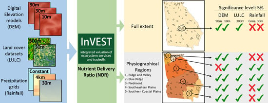
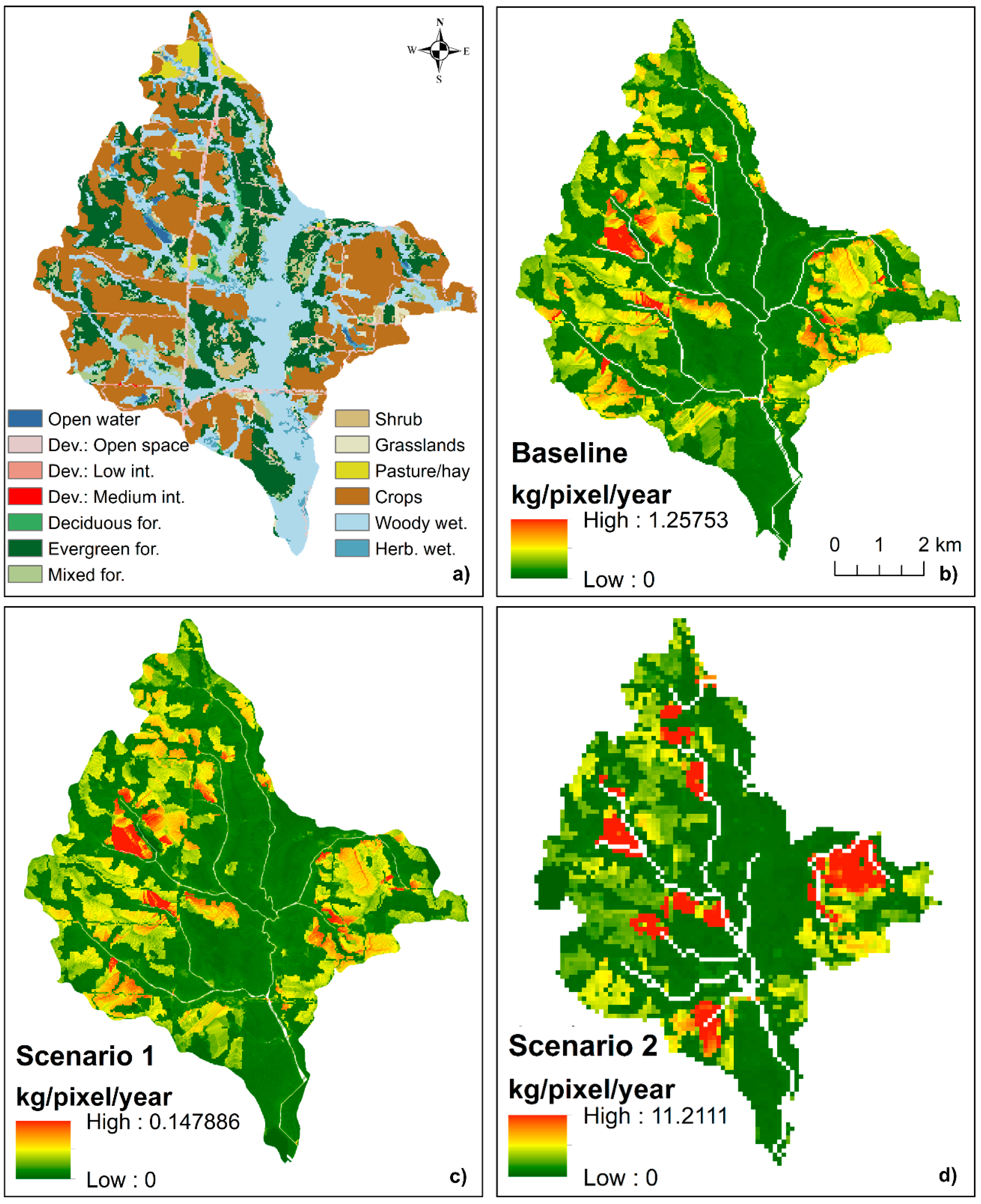
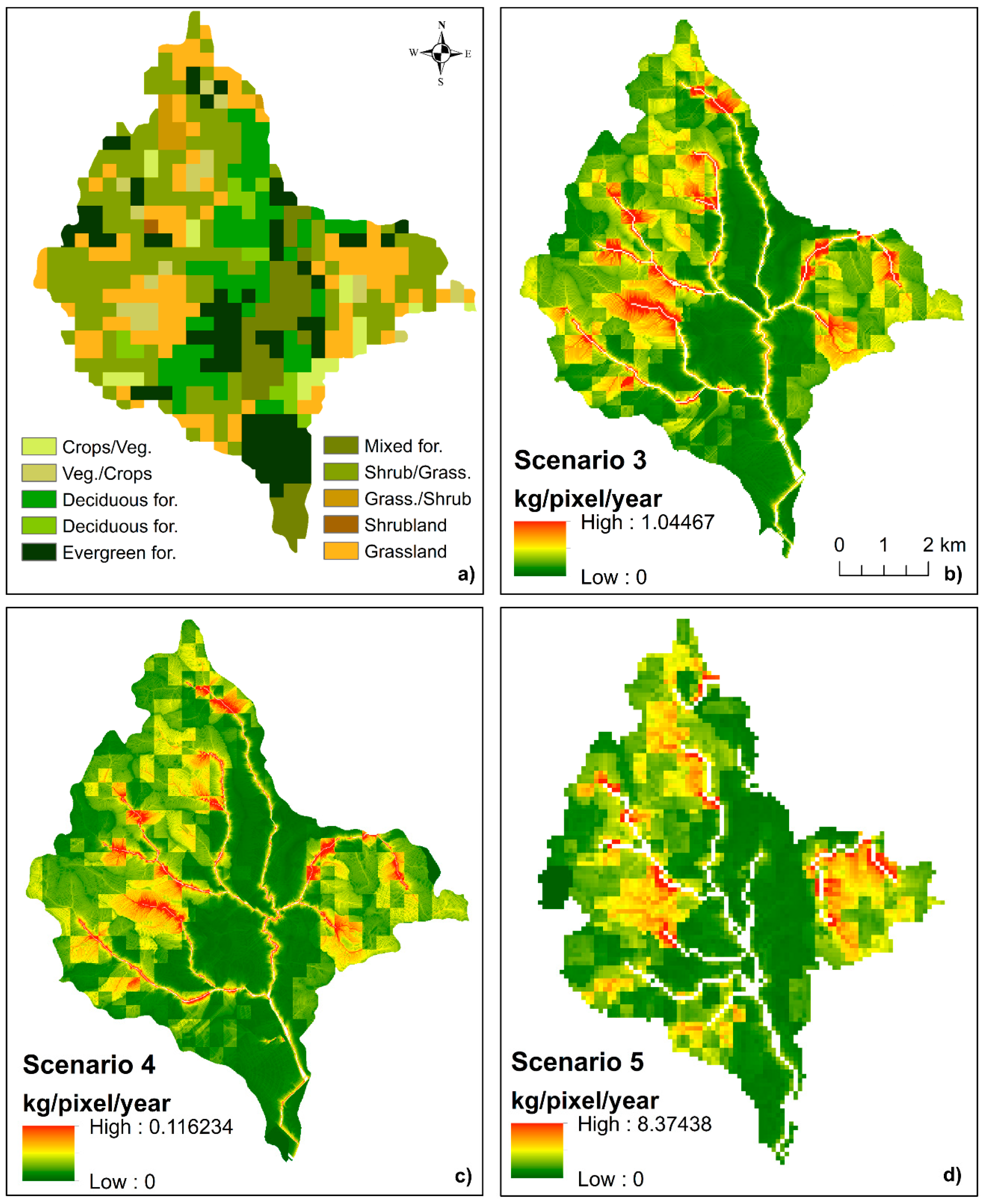
To assist practitioners in addressing the role that different scales play on ES modeling, this study used the InVEST NDR model, which maps and quantifies the delivery of nutrients (nitrogen and phosphorus) to water streams and is one of the most employed models within all the models present in InVEST. The NDR model was used for investigating the joint effects of resolution of input spatial data (land cover, DEM, and precipitation) and spatial extent on the outputs generated by this model under common modeling assumptions. This study focused on a set of 57 watersheds divided into six physiographical regions [25] located within the state of Georgia in the southern USA and covering more than half a million hectares. The developed understanding about the impact of scale on ESs would directly feed into landscape level planning processes which will further guide practices for managing natural resources in a manner where ESs are not only maintained but enhanced for society welfare.

2. Materials and Methods

2.1. Study Area

The United States Geological Survey (USGS) hydrologic unit code (HUC) 12 watershed classification system was used to select the watersheds for the study. There are 1659 HUC 12 watersheds within the state of Georgia, and they have an average area of 8491 hectares (ha), which is adequate for nutrient delivery analysis [13]. To capture the landscape heterogeneity, 57 watersheds were randomly selected such that no watershed was further than 60 km to the nearest watershed and to the nearest weather station. Georgia is divided into six distinct physiographical regions [25], and the chosen watersheds represent variations in elevation, precipitation, land cover, and demographics across these regions (Figure 1).
The Blue Ridge region is located in the northeast of the state and is characterized by a sequence of mountains and ridges covered by forest, with an elevation ranging from 480 to 1410 m. Within this region, 11 watersheds were selected. The Piedmont region is located in the central portion of Georgia and is the most populous region in the state, as Atlanta is located in this region. This region has vast pasture and mixed forest lands. Thirteen watersheds were selected in this area. The Ridge and Valley region, located in northwestern Georgia has most of its lands covered by pasture, and it is somehow flat, with an elevation ranging from 210 to 240 m. Five watersheds were selected from this region. The Southeastern Plains is the region with most of the agricultural lands in the state. Some important cities of Georgia are partially located in the upper part of this region, such as Augusta and Columbus. Twenty-one watersheds fell within this region. The Southern Coastal Plains is located in the south portion of the state and has an expressive acreage of wetlands. Six watersheds were selected in this region. Finally, the Southwestern Appalachians region is a relatively small area in the extreme northwest portion of the state mostly covered by forest. Only one watershed was chosen in this region. For the statistical analysis, this watershed was included with watersheds located in the Ridge and Valley region. The total area of selected watersheds was 560,910 ha.

2.2. The InVEST Nutrient Delivery Ratio Model

The modular toolset InVEST combines tabular and spatial data with biophysical models to quantify and evaluate selected ESs and is widely used in the literature [13,24,26,27,28]. This study used the InVEST NDR model version 3.4.2 for mapping and quantifying nutrient (nitrogen and phosphorus) delivery to local water streams. Although the model was modified from previous versions (3.1) to reduce the sensitivity to spatial data resolution [13], this study tested the influence of this factor on the output by creating scenarios using a variety of combinations of input spatial data and keeping other parameters constant. Spatial data resolution is especially important because the NDR model only accounts for diffuse nutrient sources (non-point sources) when mapping and quantifying nutrient delivery [10]. More details about the NDR model can be found in the InVEST User Guide [13], and alternatively in other publications that tested the sensitivity of this model mostly for changes in spatial resolution under different conditions [16,17].

2.3. Input Data for the InVEST NDR Model

2.3.1. Land Use/Land Cover

The NDR Model needs a land use/land cover raster file to represent how different classes influence the nutrient delivery to streams within a watershed. This study selected two land cover datasets to conduct the analysis, the NLCD and the Global Land Cover (GlobCover). The most recent NLCD dataset represents the year of 2011, and the last version of GlobCover is relative to 2009. Fortunately, there is an NLCD available for the year of 2006, and a GlobCover available for the year of 2005 with some data obtained in 2006. Therefore, 2006 was chosen as the base year to minimize the influence of land cover change across time on the model outputs. The NLCD has a spatial resolution of 30 m and is created by the Multi-Resolution Land Characteristics (MRLC) Consortium using circa 2006 Landsat satellite data based on a decision-tree classification [29]. This dataset uses 16 land cover classes for the conterminous United States and has an overall accuracy of 78% [30].
The European Space Agency (ESA) alongside with the Université Catholique de Louvain (Belgium) provided the GlobCover, which is a public access land cover dataset with 300 m spatial resolution covering all continents, except for Antarctica [31]. This dataset is a 19-class land cover classification system and has an overall accuracy of 73% when the weight of each land cover class is accounted for [32]. This study used the GlobCover covering the period from December 2004 to June 2006, originally created based on the ENVISAT (Environmental Satellite) mission using the MERIS (MEdium Resolution Imaging Spectrometer) sensor. Both land cover datasets and all spatial data used in this study were projected to the same coordinate system (WGS 1984 UTM Zone 17N). To illustrate the difference between these two land cover datasets, Figure 2 depicts the Wildcat Creek watershed classified according to NLCD 2006 (a) and GlobCover 2005 (b), respectively.

2.3.2. Digital Elevation Model

A critical input data of the NDR model is the DEM, as it displays the surface water flow patterns across the study area [13]. In addition, the DEM should extend beyond the boundary of the study area. The toolbox ArcHydro contained within the ESRI® ArcMap 10.5 was used to fill in sinks on DEM files, which are cells that the flow direction cannot be assigned and can cause errors in the output of the NDR model [13]. For testing the influence of DEM on the output of the NDR model, three DEMs with different resolutions (1/3 arcsec, 1 arcsec, and 5 arcsec) were selected. Both 1/3 and 1 arcsec DEM datasets were retrieved from the National Elevation Dataset (NED) provided by the USGS [33]. The NED is public domain data and is updated every two months to integrate the newest and best elevation data available. This dataset covers the conterminous United States, Hawaii, and Alaska (only lower resolution data are available to Alaska).
The 5 arcsec ASTER (Advanced Spaceborne Thermal Emission and Reflection Radiometer) GDEM (Global Digital Elevation Map) is a product of National Aeronautics and Space Administration (NASA) and Ministry of Economy, Trade, and Industry (METI) of Japan and was obtained from the online Data Pool, courtesy of the NASA Land Processes Distributed Active Archive Center (LP DAAC) [34]. Although this dataset has coarser data than the first two aforementioned DEMs, it is available at a global scale and could be an option for researchers conducting studies in countries that do not offer finer resolution DEM.
The threshold flow accumulation (TFA) is a parameter associated with the DEM, which is used to generate a water streams layer and can be calculated using the formula provided by the InVEST User Guide, which is 1 over the pixel area in km2 [13]. All DEMs used in this study, alongside their data sources, spatial resolutions, and TFAs are reported in Table 1.

2.3.3. Precipitation (Nutrient Runoff Proxy)

The dominant effect when determining the production of nutrient runoff within a watershed is the spatial variability of precipitation, and averaging the rainfall or using a single rain gauge or station to calculate precipitation will potentially decrease the accuracy of results [35]. The NDR model requires a dataset showing the spatial variability in runoff potential of the study area, which is the capacity to transport nutrient downstream. An annual precipitation grid can be used as the input data [13]. This study used three different precipitation grids. One was retrieved from PRISM (Parameter-elevation Regressions on Independent Slopes Model) Climate Group at Oregon State University [36] as a 4 km resolution raster file for the year of 2006. Climatologically-aided interpolation (CAI) was used to model the grids, which is an adequate technique to handle large variations in weather station data density for a longer time [36]. Datasets with 4 km resolution are available from the PRISM Climate Group website, along with annual datasets with an 800m spatial resolution for a fee.
The two other grids were created using rainfall data for the year of 2006 from 66 weather stations in Georgia managed by the University of Georgia Weather Network [37]. Although there are 86 weather stations within this network, 20 of them did not have rainfall data for 2006. To test the influence of the spatial distribution of rainfall across the landscape in the output of the NDR model, the average precipitation for the year of 2006 was calculated (1000.65 mm) using data from the weather stations and a homogeneous precipitation grid was created and used as one of the input precipitation grids.
Weather stations data were interpolated to create the third precipitation grid. The general idea of performing a spatial interpolation for producing a precipitation grid was to estimate regional values of rainfall to unsampled points based on data collected in the same region [38,39,40]. There are many techniques to interpolate precipitation data, and they can be divided into two groups: geostatistical and deterministic. The former connects mathematics and earth science, and a good example of the geostatistical technique is kriging, introduced by Matheron [41]. This technique uses autocorrelation for determining the relationships among measured points and interpolates values of unknown points. Deterministic techniques basically forecast rainfall to unsampled points by basing the calculations on the weight of the data collected on that region [42].
Results comparing interpolation methods differ among studies, and there is no unanimous method selected as the best interpolation method in the literature [43,44,45]. However, geostatistical methods apparently perform better than deterministic ones for annual and monthly rainfall, especially if elevation is included as a variable in the model [46,47,48,49]. Therefore, this study used one deterministic method (IDW) and four geostatistical methods (simple kriging (SK), ordinary kriging (ORK), universal kriging (UNK), and cokriging including elevation of stations (OCK)) to create five precipitation grids and chose one for the NDR model analysis.
Statistics associated with each interpolation method (Table 2) suggested OCK had the smallest difference between RMS error and ASE, and its RMS standardized was closest to 1. Since these are the most important components to select the best method [50], the OCK interpolation was used to create a 30 m spatial resolution precipitation grid for the analysis. Figure 3 shows all the weather stations used to create the precipitation grids, the watersheds selected for this study, the precipitation grid generated by the OCK model (3a), and the 4 km resolution precipitation grid retrieved from the PRISM Climate Group (3b).

2.3.4. Parameters

In addition to spatial data, the NDR model requires a series of other parameters. The Borselli kb parameter is used to calibrate the model by determining the relationship between the model itself and the hydrologic connectivity, which is the degree of connection from land patches to the stream [13]. Redhead et al. [17] conducted a sensitivity analysis and concluded that this relationship is site-specific due to different responses obtained in different catchments when a variety of kb parameters were used. However, this study had the objective to vary only spatial data rather than parameters and used the default value (2) suggested by Sharp et al. [13].
Moreover, a biophysical table containing information on nutrient loads for each land use/land cover (LULC) class is required for each different LULC dataset used. This table contains data related to nitrogen and phosphorus and requires values of nutrient load associated with LULC classes (kg/ha/year), maximum retention efficiency displaying the percentage of nutrient retained by vegetation, critical distance that a patch of LULC will retain nutrient in its maximum capacity (set to pixel resolution according to each LULC dataset), and proportion of nutrient that travels via surface and subsurface (set to default value, which is zero). If this last parameter is set to a value different than zero, then two more parameters are added to the model: subsurface maximum retention efficiency and subsurface critical length. Nutrient loads and efficiency coefficients were derived from a variety of published studies [17,51,52,53,54]. Finally, land cover classes from NLCD and GlobCover were matched and assigned with the same coefficients. The biophysical tables used in this study are available in the Appendix A.

2.4. Scenarios for the Assessment

All variations of DEM, land cover, and precipitation were combined in a unique manner to generate a total of 18 different scenarios (Table 3). Each scenario served the purpose of testing the influence of different input spatial data in the results of the NDR model. These 18 scenarios were used to run the NDR model for nitrogen and phosphorus export in all 57 watersheds of the study area. For each scenario, the total nutrient export of each watershed was quantified using the tool “Cell Statistics” of ArcMap. Finally, the relative nutrient load of each watershed was calculated dividing the total nutrient export by the area of the watershed.

2.5. Statistical Analysis

The statistical analysis of this study was conducted using the software R version 1.0.153 [55]. Twelve multivariate linear regression models (six for each nutrient: nitrogen and phosphorus) were developed for testing the significance of different input spatial data on the output of the NDR model. Two models were fit for the full study area, and the other ten tested each physiographical region in Georgia.
The relative nutrient export, represented as kilograms of nitrogen or phosphorus per hectare per year (kg/ha/yr) delivered to water streams, was first set to 100% for each watershed for the Baseline Scenario. Then, a percentage was calculated for each scenario and for each watershed with respect to the Baseline. This percentage was used as the continuous dependent variable in the regression model (“%Nut.load” in Equation (1)).
% Nut . load i = β 0 + β 1 DEM . 10 m i + β 2 DEM . 90 m i + β 3 GlobCover i + β 4 Stations i + β 5 A v g + ε i i = 1 , 2 , , 57
The independent variables were discrete indicators for the presence or absence of each spatial data used in the study, represented by “DEM.10m”, “DEM.90m”, “GlobCover”, “Stations”, and “Average” (precipitation grids) in Equation (1). All discrete indicators used the Baseline Scenario as contrast, and coefficients of Equation (1) should be interpreted as the percentage change with respect to the Baseline. Consistently, if all variables are set to zero (absence), the model yields the Baseline percentage, which should be as close to 100% as possible. All analyses were conducted using a significance level of 5% (α = 0.05).

3. Results

3.1. Overall Nutrient Export

Scenario 8, which combined a 90 m DEM with the NLCD land cover, yielded the highest aggregated nitrogen export among all the scenarios and the precipitation grid created using weather stations data (Figure 4). This scenario modeled a total export of 242,953 kg of nitrogen for all watersheds combined, which gives an average of 0.433 kg/ha/year of nitrogen. This relative nitrogen export is equivalent to 136.2% of the Baseline. The smallest nitrogen export was modeled in Scenario 16, which used a 10 m DEM combined with the GlobCover land cover and the average precipitation grid. This scenario yielded a total nitrogen export of 136,953 kg for all watersheds combined, with a relative nitrogen export of 0.244 kg/ha/year, which is equivalent to 76.8% of the Baseline.
The phosphorus export was highest in Scenario 8 (39,840 kg for all watersheds) with an average of 0.071 kg/ha/year of this nutrient being delivered to water streams (Figure 5). This export was relatively the highest among all scenarios including nitrogen and phosphorus, representing 138.4% of the Baseline. Scenario 16 yielded the smallest phosphorus export, with a total export of 14,861 kg for all watersheds combined, averaging 0.026 kg/ha/year of runoff to streams. In percentage terms, this scenario produced the overall smallest export, including nitrogen and phosphorus, yielding a result equivalent to 51.6% of the Baseline.
Overall, results for scenarios with varying the precipitation grid did not present high differences, relative to the Baseline. For example, Scenarios 6 and 12, which used the same DEM and land cover maps but different precipitation grids yielded nitrogen exports equivalent to 99.9% and 98.8% of the Baseline, respectively. Similarly, for phosphorus, these scenarios yielded very similar results, with nutrient exports equivalent to 99.9% and 97.8% of the Baseline, respectively. Clearly, the results differed when different DEMs were used, and all other variables were held constant.
Figure 6 illustrates the difference in the output caused by the DEM using the Griffin Lake–Ochlockonee River watershed extracted from the output of the NDR model to display the relative nitrogen exports relative to the Baseline for Scenarios 1 and 2. These scenarios used the NLCD land cover, PRISM precipitation grid, and DEMs with 30 m, 10 m, and 90 m spatial resolution, respectively. The spatial resolution of the NDR model output is the same as the DEM used.
Land cover is another variable that presented high variance among all scenarios. Figure 7 shows the relative nitrogen exports for Scenarios 3, 4, and 5, which are a combination of GlobCover land cover, PRISM precipitation grid, and DEMs with 30 m, 10 m, and 90 m spatial resolution, respectively. A similar nitrogen exports spatial pattern was observed in all outputs and is visible in Figure 6 and Figure 7. The same was observed for phosphorus export.

3.2. Scale of Input Spatial Data

When the full extent of the study area was considered, the NDR model was sensitive to changes in DEM and land cover at a 5% significance level (Table 4). According to the output of the regression model, reductions of 15.5% for nitrogen and 14.1% for phosphorus are expected if a DEM with 10 m spatial resolution is used relative to the 30 m DEM. On the other hand, increments of 10.6% for nitrogen and 13.5% for phosphorus are predicted when a 90 m DEM is used keeping all other variables constant. The highest impact in the NDR output modeling phosphorus export was observed for a change in land cover. When GlobCover was used, and all other variables held constant, the regression model predicted a reduction of 37.4% in this nutrient export compared to the Baseline. Finally, both precipitation grids were not significant at the 5% significance level.
To account for geographic, climate, and demographic variations across the study area, the watersheds were then divided into physiographical regions. Similar regression models were fit for each of the five regions, with the percentage of nutrient export with respect to the Baseline serving as the dependent variable, and the presence or absence of input spatial data being the independent indicator variables. Replacing the 30 m DEM used in the Baseline by a 10 m DEM significantly impacted the output of all models, causing a decrease in the nitrogen export (Table 5). When a 90 m DEM was used, a significant increase in export was predicted in all regions, except by the Blue Ridge, where this variable was not significant.
Land cover was significant in all regions, but when GlobCover was used in the Blue Ridge region, an export increase of 8.2% was predicted, while all other regions had negative predictions for this variable. The weather stations precipitation grid was significant in two regions, predicting a negative change of 13.2% in nitrogen export for the Blue Ridge, and an increase of 9.4% in Piedmont. The grid using the average rainfall was significant in four regions, with a negative prediction of 26.7% for the Blue Ridge, and a positive prediction of 13.5% for the Southern Coastal Plains. All regional nitrogen models had higher R2 (proportion of the variance in the dependent variable explained by the independent variables) compared to the nitrogen model fit to all watersheds (R2 = 0.232). The Southern Coastal Plains model presented the highest R2 among all nitrogen models (R2 = 0.632).
The same approach was followed for estimating phosphorus export in all five regions, but results had some important differences compared to nitrogen (Table 6). The 10 m DEM was significant in four models when replacing the 30 m DEM of the Baseline, causing a negative impact in the phosphorus export, while the 90 m DEM significantly impacted three models, but with positive effect in the output. Land cover was significant in all regions, except for the Southern Coastal Plains, with GlobCover causing a negative impact of 61.72% in the Ridge/Appalachian model, which was the highest impact across all models, including nitrogen. The precipitation grid using weather stations data was significant in two regions, predicting a negative change of 11.7% in the Blue Ridge model, and an increase of 8.2% in the Piedmont model.
The average precipitation grid was significant only in the Blue Ridge model, predicting a decrease of 23.8% in phosphorus export. Two regional phosphorus models yielded lower R2 than the model using all watersheds (R2 = 0.345), and the highest R2 among all models, including nitrogen, was observed in the Ridge/Appalachian phosphorus model (R2 = 0.878). All p-values of nitrogen and phosphorus regional models were significant, suggesting a relationship between independent variables and the dependent variables.

4. Discussion

This study aimed to provide information to researchers on how the results of the NDR model can vary with respect to the resolution of spatial data and spatial extent. A total of three DEMs, two land cover datasets, and three precipitation grids were used in unique combinations as input spatial data for the model. All parameters required, except by TFA which was calculated according to DEM spatial resolution as suggested by Sharp et al. [13], were set the same across all scenarios, so the variation in the output can be attributed solely to different spatial data used. A control scenario (Baseline) using a 30 m DEM, the NLCD land cover, and the precipitation grid retrieved from PRISM was set. Suitable multivariate regression models were employed to verify the influence of the spatial resolution of input data on the NDR model output at two spatial extents (the state of Georgia and six physiographical regions within the state).
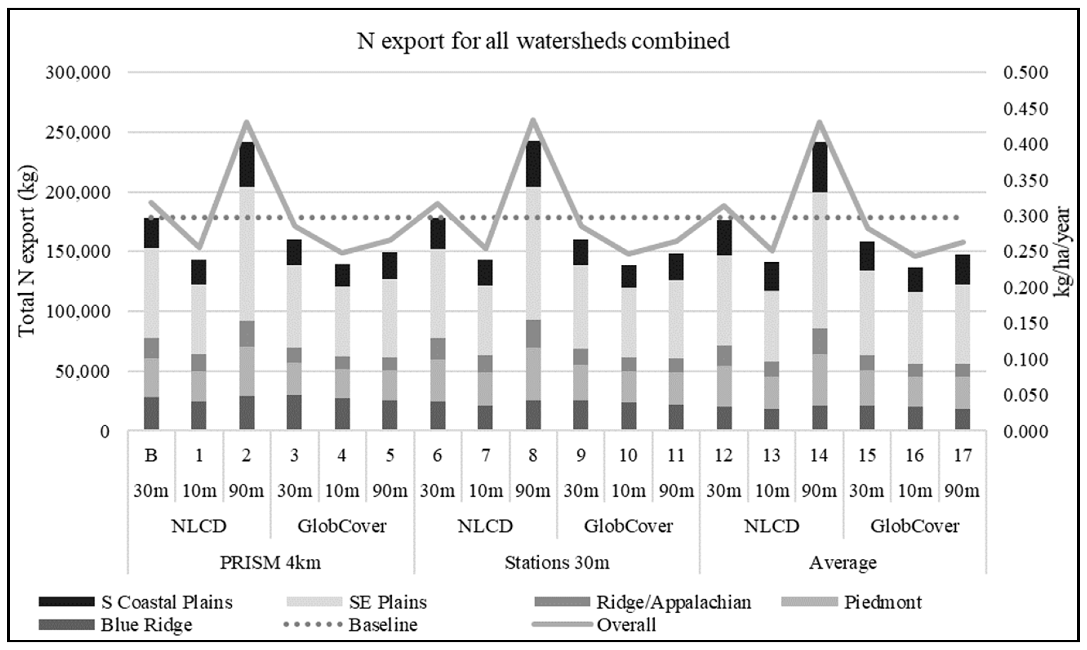
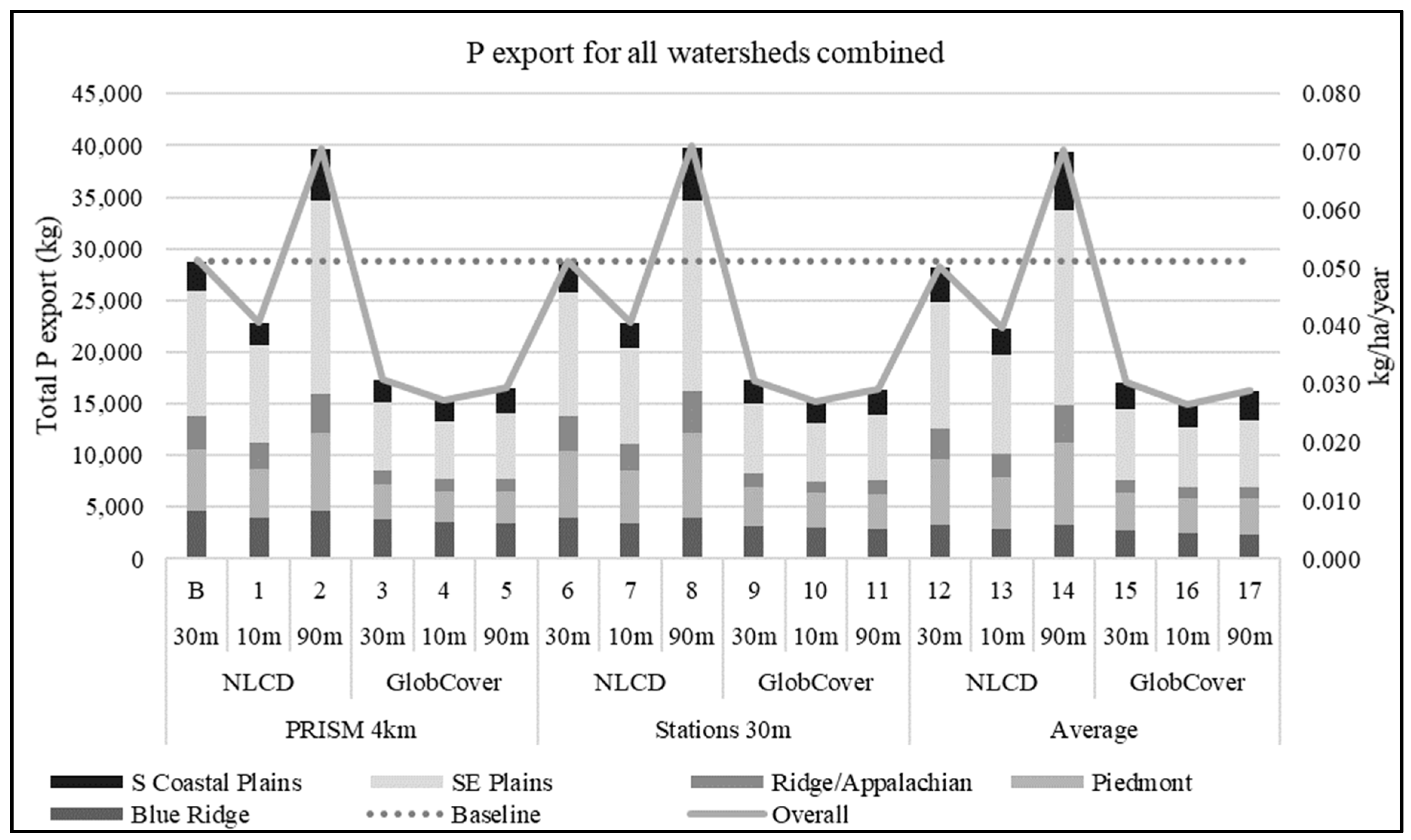
Although the nitrogen and phosphorus export fit models for all watersheds had low R2 (nitrogen: 0.232 and phosphorus: 0.345), DEM and land cover were significant at a 5% significance level. The model may not be used to precisely predict the percentage of nutrient export according to changes in spatial data resolution, but as the F-statistic and p-value of both nitrogen and phosphorus models indicated, there was a relationship among independent variables and the dependent variable, which can certainly be interpreted as an evidence that these DEM and land cover datasets significantly affected the nutrient export.
Consistently with other studies [16,17], changes in DEM caused a significant impact on the output, but the direction of this impact varied across models. Nutrient export of scenarios using NLCD was highest when the 90 m DEM were used, and lowest for 10 m DEM for all watersheds. Alternatively, a different trend was observed in scenarios using the GlobCover, where highest exports were modeled in 30 m DEM scenarios and lowest in 10 m DEM scenarios. These results indicated finer DEM resolutions do not necessarily imply higher or lower nutrient export, and it was not possible to devise an absolute trend regarding DEM resolution for the full study area.
When regression models were fit using watersheds grouped by physiographical regions, the 90 m DEM was not significant predicting nitrogen exports only in the Blue Ridge, while this variable was not significant in the aforementioned region and Piedmont for phosphorus, which indicated that replacing the 30 m DEM by the 90 m DEM did not have a significant impact in the output of these regions. The outputs of both nutrients for the other three regions were significantly affected when the 90 m DEM was used, with these models predicting an increase in nutrient export relative to the Baseline. The presence of the 10 m DEM had a negative effect in all models but was not found significant in the model predicting phosphorus export in the Southern Coastal Plains region. In addition, models using the 10 m DEM predicted overall lowest exports when all other variables were constant in the model, suggesting that such DEM resolution may be associated with lower exports.
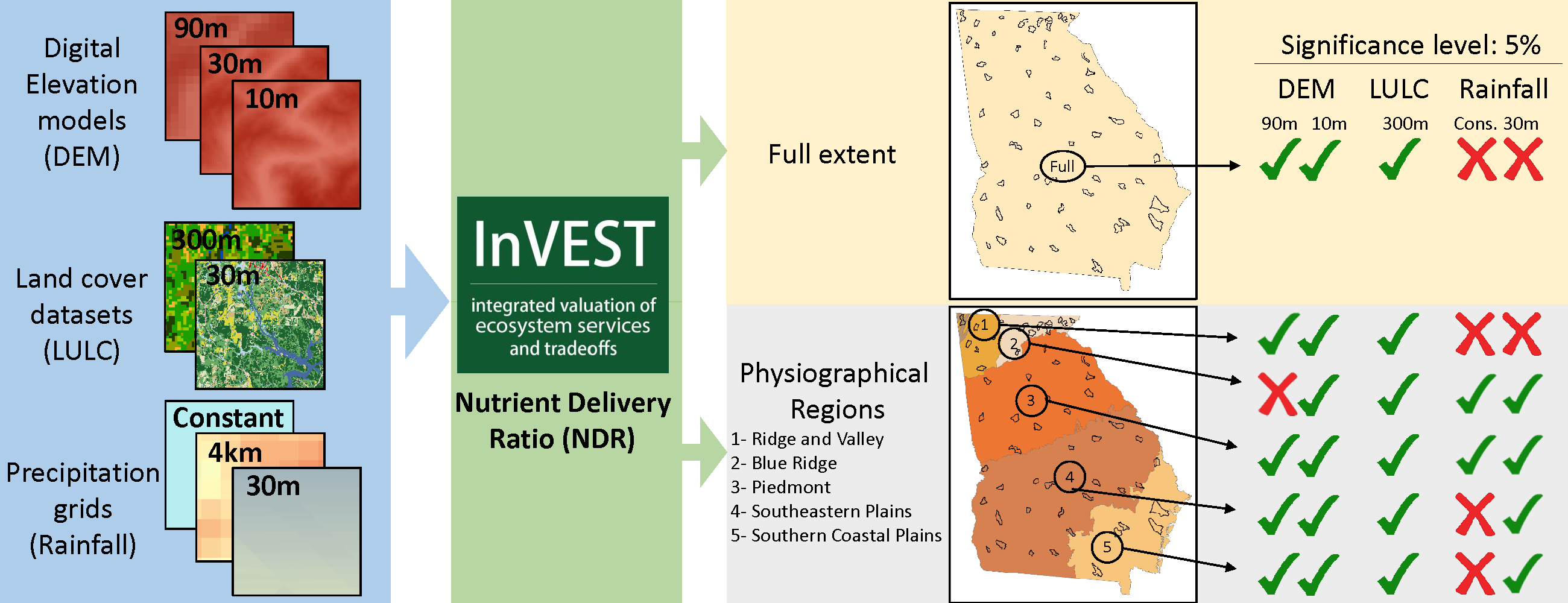
As expected due to possible inconsistencies matching land cover classes between the two datasets used in this study, and to a difference in spatial resolution, land cover significantly influenced nutrient export in both models’ fit in the full study area. Although the GlobCover is a coarser land cover dataset and consequently aggregates smaller and sparse land cover classes into more representative classes causing the disappearance of sensitive areas from the final grid, such as wetlands, this aggregation also causes agricultural, pasture, and urban lands with presence of trees and shrubs to be classified into a mosaic category, and be finally assigned lower levels of nutrient loads, as previously investigated by Avelino et al. [11] and Grêt-Regamey et al. [12].
Among all regression models predicting nutrient export for the five physiographical regions, the nitrogen model for the Blue Ridge was the only one that the presence of the GlobCover positively impacted the output. Moreover, the phosphorus model for this region was negatively impacted by this variable, but this impact was the smallest due to the presence of GlobCover in terms of magnitude. Apparently, the watersheds within this region have fragmented occurrence of agricultural and urban lands according to the NLCD, which were aggregated into more common land cover classes present in this region, such as evergreen and deciduous forest, in the GlobCover dataset. This aggregation itself would cause a nitrogen export decrease in GlobCover models outputs compared to NLCD models, due to higher nutrient loads associated with agricultural and urban lands. However, the GlobCover identifies vast areas of evergreen forests in this region while the NLCD classifies these areas mainly as deciduous forest. Since evergreen forests were assigned with higher nutrient loads, it was expected that areas covered by this class would export more nutrients to water bodies than deciduous forest areas.
The overall highest impact in regional models was predicted by the phosphorus model fit for the Ridge/Appalachian region, with an expected decrease of 61.7% when GlobCover replaced NLCD. This high decrease can be explained by differences in land cover classification in these two datasets. Many pixels that the GlobCover classified as deciduous forest in this region were classified as pasture by the NLCD and consequently assigned with very distinct nutrient loads. The Southern Coastal Plains nitrogen regional model was negatively affected by GlobCover, which was not significant for phosphorus. Vast wetlands areas identified by NLCD in this region were classified mostly as mixed or evergreen forest, less often as deciduous, by GlobCover. Although lower nutrient loads were assigned to wetlands compared to forests, and an increase in the nutrient export was expected when using GlobCover, agricultural lands were mostly classified into mosaic categories or grasslands and assigned lower nutrient loads, resulting in this predicted decrease.
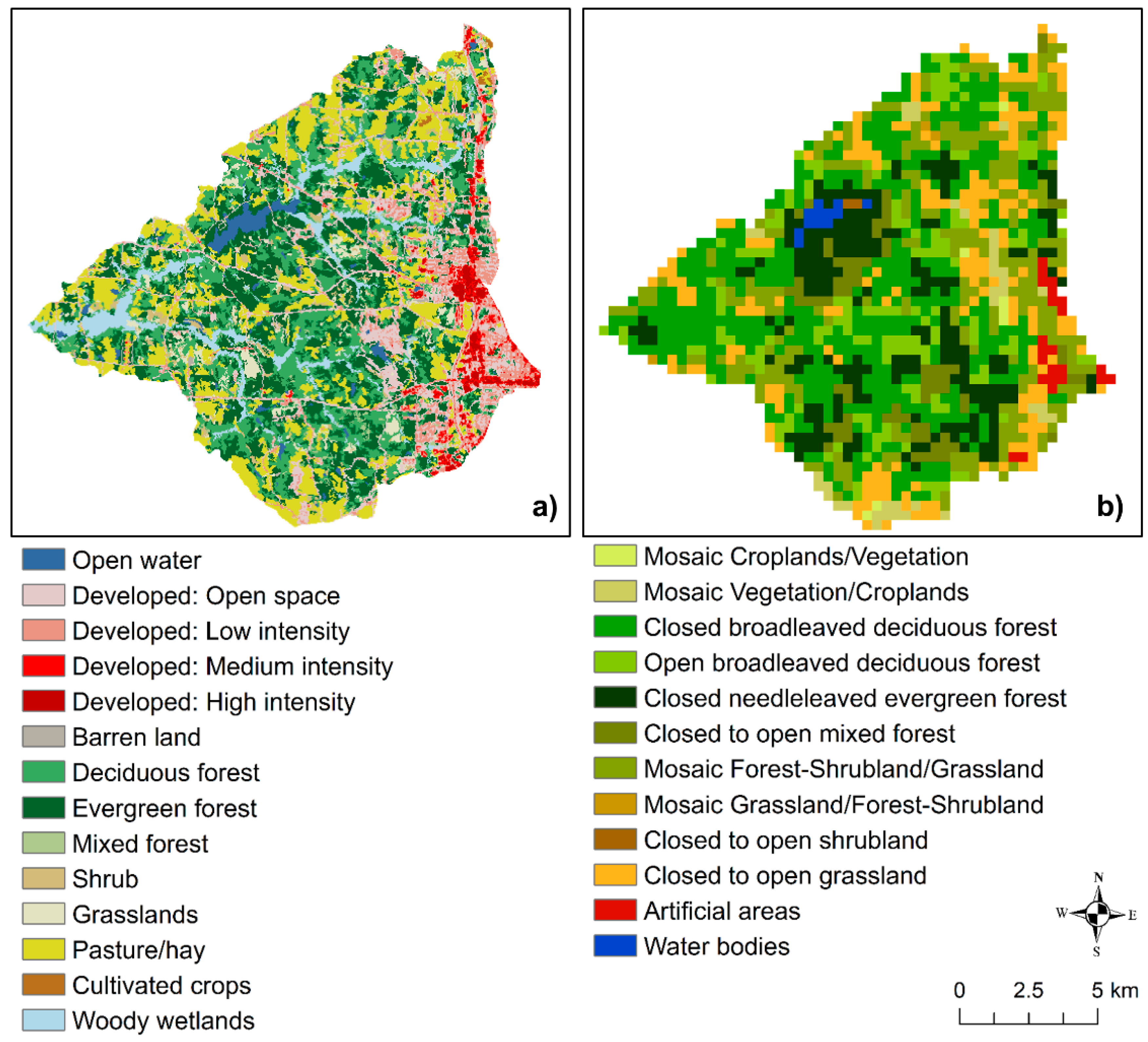
Three precipitation grids were tested to verify the influence of rainfall modeling nutrient exports using the NDR model. The PRISM grid was used in the Baseline Scenario, but when it was replaced by other grids, no significant effect was observed in the output for all watersheds combined. As shown in Figure 3, this grid had a similar spatial distribution compared to the grid created using data collected from weather stations in Georgia. Due to this similar distribution, results were not expected to vary drastically in scenarios switching only these two spatial data as suggested by Redhead et al. [17], and in fact, this lack of variation was observed for the models using all watersheds of the study area. The average precipitation grid had an obvious different distribution compared to the others, and it was expected that these differences would be reflected in the outputs, causing a significant change in nutrient exports predictions. Surprisingly, this precipitation grid was not significant for all watersheds combined, suggesting that all precipitation grids used in this study yielded overall similar results by holding all other variables at constant values.
Results were clearly different when watersheds were grouped according to physiographical regions. For both nitrogen and phosphorus export, the precipitation grid created using weather stations data was significant in two regions (Blue Ridge and Piedmont), indicating that although the rainfall distribution looks similar in these two grids, this distribution was different enough in these two regions for significantly changing the outputs for both nutrients. The Blue Ridge region historically has the highest annual average precipitation in the state [37]. Since the NDR model relates the average of the precipitation grid with the pixel value for rainfall to account for runoff potential [13], regions with extreme values of precipitation within the study area, such as the Blue Ridge, may be more sensitive to changes in precipitation grid. The PRISM grid provided the highest rainfall for this region compared to the other two grids. This is consistent with the coefficients of the regional model for this region, which predicted a decrease in nitrogen and phosphorus exports when the PRISM grid was replaced by the weather stations grid.
Regional models outputs for nitrogen exports were significantly influenced by the replacement of the PRISM grid by the average grid in all regions, except Ridge/Appalachian. It was observed that in drier regions, such as the Southern Coastal Plains, this grid was significant with a positive coefficient, indicating that when the average grid was used in this region, an increase in nitrogen export was predicted compared to results using the PRISM grid. Moreover, the regional model of the Blue Ridge, which has a precipitation level above the average, predicted a negative coefficient for the presence of the average grid, suggesting a significant decrease in nitrogen export compared to the presence of PRISM. This was somehow expected because the average grid leveled out rainfall across all regions. However, the presence of the average grid was not significant in four of the regional phosphorus models. This grid significantly affected only the Blue Ridge model, predicting a decrease when the PRISM was replaced by the average grid.

5. Conclusions

InVEST models are experiencing an increase in popularity, and many studies have been using them to quantify and valuate ESs for a variety of reasons, such as policy-making and scientific research. Sensitivity analyses of these models help the users’ community to understand possible changes in the outputs caused by variations in input data. This study provided an analysis on how the results of the NDR model were affected by variations in the required input spatial data, which are DEM, land cover, and precipitation. In addition, the influence of these spatial variables under two different extents were analyzed. Overall, the DEMs used in this study caused a significant impact on the model’s output. However, this impact did not follow a consistent trend across spatial resolution and extent.
The results in both extents were significantly affected by the two land cover datasets. These changes could have been caused mainly by inconsistency when matching the land cover classes of these two datasets or by differences in land cover classification itself. The GlobCover is a coarse dataset and aggregates less representative areas into broad classes. This aggregation can cause both negative and positive changes in the NDR model’s output compared to finer resolution datasets (e.g., NLCD). Classes assigned with low nutrient loads, such as wetlands, can be incorporated into more common classes assigned with higher nutrient loads, such as forests. Alternatively, agricultural fields, pasture, and low intensity developed areas can be classified as a mosaic of vegetation, being assigned with lower nutrient loads. The precipitation grids used to analyze the model did not significantly impact the output when used in the full extent of the study area. However, different grids yielded distinct results in some models applied to physiographical regions in Georgia.
Our study clearly indicates that the resolution and extent of the input data could significantly affect the quantification of ESs. This further suggests that policymakers should be cognizant about the resolution and extent of input data used in any analysis before using the same for policies on ESs. There also exists a need for better empirical data on nutrient export for further demonstrating the influence of resolution of input spatial data and extent using the NDR model or other similar models for quantifying and validating the models. We hope that this study will guide future research on ESs for informed policymaking in the context of ESs worldwide.

Author Contributions

Conceptualization, F.J.B.-S.; methodology, F.J.B.-S. and P.D.; software, F.J.B.-S.; formal analysis, F.J.B.-S. and P.D.; investigation, F.J.B.-S. and P.D.; resources, F.J.B.-S. and P.D.; writing—original draft preparation, F.J.B.-S.; writing—review and editing, P.D.

Funding

This research received no external funding.

Acknowledgments

We thank Marguerite Madden for her thoughtful insights during the conceptualization of this study.

Conflicts of Interest

The authors declare no conflict of interest.

Appendix A

Table A1. Biophysical table used for scenarios using the NLCD land cover dataset.
LucodeLULC_descload_neff_nload_peff_p
24Developed, High intensity14.950.074.850.05
23Developed Medium intensity12.780.084.170.05
82Cultivated crops12.420.252.210.25
81Pasture/Hay6.280.11.350.25
71Grasslands/Herbaceous5.670.60.150.4
22Developed, Low intensity4.970.090.530.05
52Shrub/Scrub30.650.150.4
21Developed, Open Space2.60.10.180.05
42Evergreen forest2.380.80.2980.8
43Mixed forest2.20.830.2750.8
41Deciduous forest20.850.250.8
90Woody wetlands1.30.70.070.8
95Emergent herbaceous wetlands1.50.60.080.8
31Bare rock/Sand/Clay10.050.10.05
11Water0000
Other parameters kept constant in all land cover classes: “crit_len_n”: 30, “crit_len_p”: 30 and “proportion_subsurface_n”: 0.
Table A2. Biophysical table used for scenarios using the GlobCover land cover dataset.
LucodeLULC_descload_neff_nload_peff_p
190Artificial surfaces (Urban areas >50%)12.780.084.850.05
11Post-flooding/irrigated croplands (or aquatic)12.420.252.210.25
14Rainfed croplands12.420.252.210.25
20Mosaic cropland (50–70%)/natural vegetation (20–50%)6.280.11.350.25
30Mosaic natural vegetation (50–70%)/cropland (20–50%)5.670.60.150.4
120Mosaic grassland (50–70%)/forest or shrubland (20–50%)5.670.60.150.4
140Closed to open (>15%) herbaceous vegetation5.670.60.150.4
110Mosaic forest or shrubland (50–70%)/grassland (20–50%)30.650.150.4
130Closed to open (>15%) shrubland (<5m)30.650.150.4
150Sparse (<15%) vegetation30.650.150.4
70Closed (>40%) needleleaved forest (>5m)2.380.80.2980.8
40Closed to open (>15%) broadleaved forest (>5m)2.20.830.2750.83
90Open (15–40%) needleleaved forest (>5m)2.20.830.2750.83
100Closed to open (>15%) mixed forest (>5m)2.20.830.2750.83
50Closed (>40%) broadleaved forest (>5m)20.850.250.8
60Open (15–40%) broadleaved forest (>5m)20.850.250.8
160Closed to open (>15%) broadleaved forest regularly flooded1.30.70.070.8
170Closed (>40%) broadleaved forest/shrubland permanently flooded1.30.70.070.8
180Closed to open (>15%) grassland/woody vegetation regularly flooded1.50.60.080.8
200Bare areas10.050.10.05
210Water bodies0100
Other parameters kept constant in all land cover classes: “crit_len_n”: 290, “crit_len_p”: 290 and “proportion_subsurface_n”: 0.

References

  1. Millennium Ecosystem Assessment. Millennium Ecosystem Assessment Synthesis Report; Island Press: Washington, DC, USA, 2005. [Google Scholar]
  2. Sukhdev, P. The Economics of Ecosystems & Biodiversity: An Interim Report; European Union Commission for the Environment: Brüssel, Belgium, 2008. [Google Scholar]
  3. Costanza, R.; de Groot, R.; Sutton, P.; van der Ploeg, S.; Anderson, S.J.; Kubiszewski, I.; Farber, S.; Turner, R.K. Changes in the global value of ecosystem services. Glob. Environ. Change 2014, 26, 152–158. [Google Scholar] [CrossRef]
  4. Costanza, R.; D’Arge, R.; de Groot, R.; Farber, S.; Grasso, M.; Hannon, B.; Limburg, K.; Naeem, S.; O’Neill, R.V.; Paruelo, J.; et al. The value of the world’s ecosystem services and natural capital. Nature 1997, 387, 253–260. [Google Scholar] [CrossRef]
  5. de Groot, R.; Brander, L.; van der Ploeg, S.; Costanza, R.; Bernard, F.; Braat, L.; Christie, M.; Crossman, N.; Ghermandi, A.; Hein, L.; et al. Global estimates of the value of ecosystems and their services in monetary units. Ecosyst. Serv. 2012, 1, 50–61. [Google Scholar] [CrossRef] [Green Version]
  6. Chen, N.; Li, H.; Wang, L. A GIS-based approach for mapping direct use value of ecosystem services at a county scale: Management implications. Ecol. Econ. 2009, 68, 2768–2776. [Google Scholar] [CrossRef]
  7. Daily, G.C.; Polasky, S.; Goldstein, J.; Kareiva, P.M.; Mooney, H.A.; Pejchar, L.; Ricketts, T.H.; Salzman, J.; Shallenberger, R. Ecosystem services in decision making: Time to deliver. Front. Ecol. Environ. 2009, 7, 21–28. [Google Scholar] [CrossRef]
  8. Malinga, R.; Gordon, L.J.; Jewitt, G.; Lindborg, R. Mapping ecosystem services across scales and continents—A review. Ecosyst. Serv. 2015, 13, 57–63. [Google Scholar] [CrossRef]
  9. Raudsepp-Hearne, C.; Peterson, G.D. Scale and ecosystem services: How do observation, management, and analysis shift with scale—Lessons from Québec. Ecol. Soc. 2016, 21. [Google Scholar] [CrossRef]
  10. Sharps, K.; Masante, D.; Thomas, A.; Jackson, B.; Redhead, J.; Prosser, H.; Cosby, B.; Emmett, B.; Jones, L. Comparing strengths and weaknesses of three ecosystem services modelling tools in a diverse UK river catchment. Sci. Total Environ. 2017, 584–585, 118–130. [Google Scholar] [CrossRef] [PubMed]
  11. Avelino, A.F.T.; Baylis, K.; Honey-Rosés, J. Goldilocks and the raster grid: Selecting scale when evaluating conservation programs. PLoS ONE 2016, 11, 1–24. [Google Scholar] [CrossRef]
  12. Grêt-Regamey, A.; Weibel, B.; Bagstad, K.J.; Ferrari, M.; Geneletti, D.; Klug, H.; Schirpke, U.; Tappeiner, U. On the effects of scale for ecosystem services mapping. PLoS ONE 2014, 9, 1–26. [Google Scholar] [CrossRef]
  13. Sharp, R.; Tallis, H.T.; Ricketts, T.; Guerry, A.D.; Wood, S.A.; Chaplin-Kramer, R.; Nelson, E.; Ennaanay, D.; Wolny, S.; Olwero, N.; et al. InVEST +VERSION 3.4.0+ User’s Guide; The Natural Capital Project, Stanford University: Stanford, CA, USA; University of Minnesota: Minneapolis, MN, USA; The Nature Conservancy: Arlington County, VA, USA; World Wildlife Fund: Gland, Switzerland, 2016. [Google Scholar]
  14. Kandziora, M.; Burkhard, B.; Müller, F. Mapping provisioning ecosystem services at the local scale using data of varying spatial and temporal resolution. Ecosyst. Serv. 2013, 4, 47–59. [Google Scholar] [CrossRef]
  15. Konarska, K.M.; Sutton, P.C.; Castellon, M. Evaluating scale dependence of ecosystem service valuation: A comparison of NOAA-AVHRR and Landsat TM datasets. Ecol. Econ. 2002, 41, 491–507. [Google Scholar] [CrossRef]
  16. Salata, S.; Garnero, G.; Barbieri, C.; Giaimo, C. The integration of ecosystem services in planning: An evaluation of the Nutrient Retention Model using InVEST software. Land 2017, 6, 48. [Google Scholar] [CrossRef]
  17. Redhead, J.W.; May, L.; Oliver, T.H.; Hamel, P.; Sharp, R.; Bullock, J.M. National scale evaluation of the InVEST nutrient retention model in the United Kingdom. Sci. Total Environ. 2018, 610–611, 666–677. [Google Scholar] [CrossRef] [PubMed]
  18. Fu, B.; Liang, D.; Lu, N. Landscape ecology: Coupling of pattern, process, and scale. Chinese Geogr. Sci. 2011, 21, 385–391. [Google Scholar] [CrossRef]
  19. Eppink, F.V.; Werntze, A.; Mäs, S.; Popp, A.; Seppelt, R. Land Management and Ecosystem Services. How Collaborative Research Programmes Can Support Better Policies; Oekom Verlag: Munich, Germany, 2012; Volume 1, pp. 55–63. [Google Scholar]
  20. Crossman, N.D.; Burkhard, B.; Nedkov, S.; Willemen, L.; Petz, K.; Palomo, I.; Drakou, E.G.; Martín-Lopez, B.; McPhearson, T.; Boyanova, K.; et al. A blueprint for mapping and modelling ecosystem services. Ecosyst. Serv. 2013, 4, 4–14. [Google Scholar] [CrossRef]
  21. Bagstad, K.J.; Cohen, E.; Ancona, Z.H.; Mcnulty, S.G.; Sun, G. The sensitivity of ecosystem service models to choices of input data and spatial resolution. Appl. Geogr. 2018, 93, 25–36. [Google Scholar] [CrossRef]
  22. Krueger, E.; Jordan, N. Preserving Water Quality in the Savannah River. Available online: https://s3.amazonaws.com/tnc-craft/library/Savannah-Potable-White-Paper-Final-091614.pdf?mtime=20180822151837 (accessed on 19 April 2019).
  23. Brown, M.G.; Quinn, J.E. Zoning does not improve the availability of ecosystem services in urban watersheds. A case study from Upstate South Carolina, USA. Ecosyst. Serv. 2018, 34, 254–265. [Google Scholar] [CrossRef]
  24. Butsic, V.; Shapero, M.; Moanga, D.; Larson, S. Using InVEST to assess ecosystem services on conserved properties in Sonoma County, CA. Calif. Agric. 2017, 71, 81–89. [Google Scholar] [CrossRef] [Green Version]
  25. Hodler, T.W.; Schretter, H.A. The Atlas of Georgia; University of Georgia Press: Athens, GA, USA, 1986. [Google Scholar]
  26. Nelson, E.; Mendoza, G.; Regetz, J.; Polasky, S.; Tallis, H.; Cameron, D.R.; Chan, K.M.A.; Daily, G.C.; Goldstein, J.; Kareiva, P.M.; et al. Modeling multiple ecosystem services, biodiversity conservation, commodity production, and tradeoffs at landscape scales. Front. Ecol. Environ. 2009, 7, 4–11. [Google Scholar] [CrossRef] [Green Version]
  27. Polasky, S.; Nelson, E.; Pennington, D.; Johnson, K.A. The impact of land-use change on ecosystem services, biodiversity and returns to landowners: A case study in the state of Minnesota. Environ. Resour. Econ. 2011, 48, 219–242. [Google Scholar] [CrossRef]
  28. Kovacs, K.; Polasky, S.; Nelson, E.; Keeler, B.L.; Pennington, D.; Plantinga, A.J.; Taff, S.J. Evaluating the return in ecosystem services from investment in public land acquisitions. PLoS ONE 2013, 8, 1–17. [Google Scholar] [CrossRef] [PubMed]
  29. Fry, J.; Xian, G.; Jin, S.; Dewitz, J.; Homer, C.; Yang, L.; Barnes, C.; Herold, N.; Wickham, J. Completion of the 2006 National Land Cover Database for the conterminous United States. Photogramm. Eng. Remote Sens. 2011, 77, 858–864. [Google Scholar]
  30. Wickham, J.D.; Stehman, S.V.; Gass, L.; Dewitz, J.; Fry, J.A.; Wade, T.G. Accuracy assessment of NLCD 2006 land cover and impervious surface. Remote Sens. Environ. 2013, 130, 294–304. [Google Scholar] [CrossRef]
  31. ESA. GlobCover 2005. Available online: http://due.esrin.esa.int/page_globcover.php (accessed on 19 April 2019).
  32. Defourny, P.; Schouten, L.; Bartalev, S.; Bontemps, S.; Caccetta, P.; Bella, C.D.; Gond, V.; Hazeu, G.W.; Heinimann, A.; Herold, M.; et al. Accuracy Assessment of a 300 m Global Land Cover Map: The GlobCover Experience. In Proceedings of the 33rd International Symposium on Remote Sensing of Environment, Sustaining the Millennium Development Goals, Stresa, Italy, 4–9 May 2009. [Google Scholar]
  33. Gesch, D.B.; Evans, G.A.; Oimoen, M.J.; Arundel, S. The National Elevation Dataset (NED); American Society for Photogrammetry and Remote Sensing: Bethesda, MD, USA, 2018. [Google Scholar]
  34. NASA, METI. ASTER Global Digital Elevation Model (GDEM) v2 data. Available online: https://gdex.cr.usgs.gov/gdex/ (accessed on 19 April 2019).
  35. Segond, M.-L.; Wheater, H.S.; Onof, C. The significance of spatial rainfall representation for flood runoff estimation: A numerical evaluation based on the Lee catchment, UK. J. Hydrol. 2007, 347, 116–131. [Google Scholar] [CrossRef]
  36. PRISM Climate Group. 4 km Resolution Annual Precipitation. Available online: http://prism.oregonstate.edu/ (accessed on 19 April 2019).
  37. University of Georgia Weather Network. Georgia Weather Stations. Available online: http://www.georgiaweather.net/ (accessed on 19 April 2019).
  38. Caruso, C.; Quarta, F. Interpolation methods comparison. Comput. Math. Appl. 1998, 35, 109–126. [Google Scholar] [CrossRef] [Green Version]
  39. Lanza, L.G.; Ramírez, J.A.; Todini, E. Stochastic rainfall interpolation and downscaling. Hydrol. Earth Syst. Sci. 2001, 5, 139–143. [Google Scholar] [CrossRef] [Green Version]
  40. Ly, S.; Charles, C.; Degré, A. Different methods for spatial interpolation of rainfall data for operational hydrology and hydrological modeling at watershed scale: a review. Biotechnol. Agron. Société. Environ. 2013, 17, 392–406. [Google Scholar]
  41. Matheron, G. The Theory of Regionalized Variables and its Applications; Ecole Nationale Superieure des Mines de Paris: Paris, France, 1971. [Google Scholar]
  42. Nalder, I.A.; Wein, R.W. Spatial interpolation of climatic Normals: Test of a new method in the Canadian boreal forest. Agric. Meteorol. 1998, 92, 211–225. [Google Scholar] [CrossRef]
  43. Dirks, K.N.; Hay, J.E.; Stow, C.D.; Harris, D. High-resolution studies of rainfall on Norfolk Island. Part II: Interpolation of rainfall data. J. Hydrol. 1998, 208, 187–193. [Google Scholar] [CrossRef]
  44. Ruelland, D.; Ardoin-Bardin, S.; Billen, G.; Servat, E. Sensitivity of a lumped and semi-distributed hydrological model to several methods of rainfall interpolation on a large basin in West Africa. J. Hydrol. 2008, 361, 96–117. [Google Scholar] [CrossRef]
  45. Masih, I.; Maskey, S.; Uhlenbrook, S.; Smakhtin, V. Assessing the impact of areal precipitation input on streamflow simulations using the SWAT model. J. Am. Water Resour. Assoc. 2011, 47, 179–195. [Google Scholar] [CrossRef]
  46. Goovaerts, P. Geostatistical approaches for incorporating elevation into the spatial interpolation of rainfall. J. Hydrol. 2000, 228, 113–129. [Google Scholar] [CrossRef] [Green Version]
  47. Diodato, N. The influence of topographic co-variables on the spatial variability of precipitation over small regions of complex terrain. Int. J. Climatol. 2005, 25, 351–363. [Google Scholar] [CrossRef] [Green Version]
  48. Basistha, A.; Arya, D.S.; Goel, N.K. Spatial distribution of rainfall in Indian Himalayas—A case study of Uttarakhand Region. Water Resour. Manag. 2008, 22, 1325–1346. [Google Scholar] [CrossRef]
  49. Moral, F.J. Comparison of different geostatistical approaches to map climate variables: Application to precipitation. Int. J. Climatol. 2010, 30, 620–631. [Google Scholar] [CrossRef]
  50. Webster, R.; Oliver, M.A. Geostatistics for Environmental Scientists, 2nd ed.; John Wiley & Sons, Ltd.: West Sussex, UK, 2007. [Google Scholar]
  51. Reckhow, K.H.; Beaulac, M.N.; Simpson, J.T. Modeling phosphorus loading response under uncertain. A manual and compilation of export coefficients. Water Resour. Res. 1980, 30, 1–214. [Google Scholar]
  52. Northeast Florida Water Management District. St. Marks and Wakulla Rivers Resource Assessment and Greenway Protection Plan; United States Government Printing Office: Washington, DC, USA, 1994.
  53. Harmel, D.; Potter, S.; Casebolt, P.; Reckhow, K.; Green, C.; Haney, R. Compilation of measured nutrient load data for agricultural land uses in the United States. J. Am. Water Resour. Assoc. 2006, 42, 1163–1178. [Google Scholar] [CrossRef]
  54. Jeje, Y. Export coefficients for total phosphorus, total nitrogen and total suspended solids in the Southern Alberta Region—A review of literature. Alberta Environ. 2006, 27, 1–22. [Google Scholar]
  55. Core Team, R. R: A Language and Environment for Statistical Computing; R Foundation for Statistical Computing: Vienna, Austria, 2014. [Google Scholar]
Figure 1. The full extent of the study area is a set of 57 watersheds within the state of Georgia in southern United States. Georgia can be divided in six physiographical regions, as displayed on the map. The Wildcat Creek and Griffin Lake–Ochlockonee River watersheds are highlighted on the map as they are mentioned in the text.
Environments 06 00052 g001
Figure 2. The Wildcat Creek watershed represented by the NLCD 2006 (a) as a land cover map with 30 m spatial resolution (https://www.mrlc.gov/nlcd2006.php), and by the GlobCover 2005 (b) with 300 m spatial resolution (© ESA 2010 and UCLouvain. http://due.esrin.esa.int/page_globcover.php).
Environments 06 00052 g002
Figure 3. Precipitation grid with 30 m spatial resolution created interpolating rainfall and elevation (cokriging) data from weather stations in Georgia (a) [37], and precipitation grid with 4 km spatial resolution created by PRISM (b) (Copyright © 2018, PRISM Climate Group, Oregon State University, http://prism.oregonstate.edu. Map created on 03/16/2018) [36]. All watersheds used in this study are displayed in both maps. Precipitation is displayed as millimeters per year.
Environments 06 00052 g003
Figure 4. Total and relative nitrogen export for all scenarios aggregated from all watersheds. The bars show the total nitrogen export (kg) broken down by physiographical regions, the line provides the overall average of relative nitrogen export (kg/ha/year), and the dotted line displays the total export yielded by the Baseline (kg).
Environments 06 00052 g004
Figure 5. Total and relative phosphorus export for all scenarios aggregated from all watersheds. The bars show the total phosphorus export (kg) broken down by physiographical regions, the line provides the overall average of relative phosphorus export (kg/ha/year), and the dotted line displays the total export yielded by the Baseline (kg).
Environments 06 00052 g005
Figure 6. Land cover of the Griffin Lake–Ochlockonee River watershed according to the NLCD (a), and the outputs of the NDR models for the Baseline (b), Scenarios 1 (c), and 2 (d) showing the nitrogen export (kg/pixel/year) to water streams within this watershed. Figure 6a,b have a spatial resolution of 30 m, Figure 6c has a spatial resolution of 10 m, and Figure 6d has a spatial resolution of 90 m.
Environments 06 00052 g006
Figure 7. Land cover of the Griffin Lake–Ochlockonee River watershed according to the GlobCover (a), and the outputs of the NDR models for the Scenarios 3 (b), 4 (c), and 5 (d) showing the nitrogen export (kg/pixel/year) to water streams within this watershed. Spatial resolutions of Figure 7a–d are 300 m, 30 m, 10 m, and 90 m, respectively.
Environments 06 00052 g007
Table 1. Digital elevation models (DEMs) with their respective data sources, spatial resolutions in arcsec and meters, and threshold flow accumulation (TFA).
SourceResolution (arcsec)Resolution (m)Threshold Flow Accumulation (TFA)
USGS 11/3~1010,000
USGS 11301111
NASA 25~90123
1 USGS: United States Geological Survey [33]. 2 NASA: National Aeronautics and Space Administration [34].
Table 2. Output displaying the statistics of deterministic and geostatistical interpolation methods used to create precipitation grids based on all available data collected from weather stations in Georgia managed by the University of Georgia Weather Network.
Interpolation Method
DeterministicGeostatistical
IDWORKSKUNKOCK
Mean−11.393−7.086−0.467−7.086−0.113
Mean Standardized-−0.037−0.001−0.0370.003
Root-Mean-Square (RMS)138.691138.921137.618138.921150.429
Root-Mean-Square Standardized-1.0051.1111.0050.996
Average Standard Error (ASE)-135.032123.152135.032150.451
Difference (RMS-ASE) 3.88914.4663.889−0.022
Abbreviations: Inverse Distance Weighting (IDW), Ordinary Kriging (ORK), Simple Kriging (SK), Universal Kriging (UNK), and Cokriging (OCK).
Table 3. Scenarios used in this study are a unique combination of input spatial data of the Nutrient Delivery Ratio (NDR) model. Digital elevation models (DEM), land cover datasets, and precipitation grids used are displayed with their respective data source and spatial resolution.
ScenarioDEMLand CoverPrecipitation
SourceResolution (m)SourceResolution (m)SourceResolution (m)
BaselineUSGS 130NLCD 2006 330PRISM 54000
1USGS 110NLCD 2006 330PRISM 54000
2NASA 290NLCD 2006 330PRISM 54000
3USGS 130GlobCover 2005 4300PRISM 54000
4USGS 110GlobCover 2005 4300PRISM 54000
5NASA 290GlobCover 2005 4300PRISM 54000
6USGS 130NLCD 2006 330Stations 630
7USGS 110NLCD 2006 330Stations 630
8NASA 290NLCD 2006 330Stations 630
9USGS 130GlobCover 2005 4300Stations 630
10USGS 110GlobCover 2005 4300Stations 630
11NASA 290GlobCover 2005 4300Stations 630
12USGS 130NLCD 2006 330Average 64000
13USGS 110NLCD 2006 330Average 64000
14NASA 290NLCD 2006 330Average 64000
15USGS 130GlobCover 2005 4300Average 64000
16USGS 110GlobCover 2005 4300Average 64000
17NASA 290GlobCover 2005 4300Average 64000
1 USGS: United States Geological Survey [33]. 2 NASA: National Aeronautics and Space Administration [34]. 3 NLCD: National Land Cover Dataset [29]. 4 GlobCover: Global Land Cover [31]. 5 PRISM: Climate Group at Oregon State University [36]. 6 Stations: University of Georgia Weather Network [37].
Table 4. Outputs of the multivariate linear regression models predicting the percentage change in nitrogen and phosphorus export (kg/ha/year) with respect to the Baseline Scenario for the full extent of the study area using input spatial data as independent variables (digital elevation model (DEM), land cover, and precipitation).
VariableNitrogenPhosphorus
Coefficientp-ValueCoefficientp-Value
Intercept105.489<0.001104.635<0.001
DEM: 10 m−15.537<0.001−14.051<0.001
DEM: 90 m10.594<0.00113.482<0.001
GlobCover−15.136<0.001−37.392<0.001
Stations1.3570.4591.0900.637
Average−0.2530.8900.0490.983
F-statistic61.68107.30
p-value<0.001<0.001
R20.2320.345
n10261026
Table 5. Outputs of the multivariate linear regression models predicting the percentage change in nitrogen export (kg/ha/year) with respect to the Baseline Scenario for the five physiographical regions of Georgia using input spatial data as independent variables (digital elevation model (DEM), land cover and precipitation).
Blue RidgePiedmontRidge/AppalachianSE PlainsS Coastal Plains
VariableCoeff.p-ValueCoeff.p-ValueCoeff.p-ValueCoeff.p-ValueCoeff.p-Value
Intercept102.093<0.001105.061<0.001104.085<0.001107.695<0.001106.322<0.001
DEM: 10 m−7.9940.029−16.881<0.001−15.550<0.001−18.562<0.001−15.851<0.001
DEM: 90 m−5.6020.1256.5800.0436.7770.04318.966<0.00123.505<0.001
GlobCover8.2210.006−16.928<0.001−33.141<0.001−16.769<0.001−30.352<0.001
Stations−13.192<0.0019.3670.0044.8700.1452.5860.3822.8640.501
Average−26.696<0.0017.3710.023−3.9730.2336.0200.04213.4730.002
F-statistic13.3421.3240.9942.7035.03
p-value<0.001<0.001<0.001<0.001<0.001
R20.2580.3190.6680.3650.632
n198234108378108
Table 6. Outputs of the multivariate linear regression models predicting the percentage change in phosphorus export (kg/ha/year) with respect to the Baseline Scenario for the five physiographical regions of Georgia using input spatial data as independent variables (digital elevation model (DEM), land cover and precipitation).
Blue RidgePiedmontRidge/AppalachianSE PlainsS Coastal Plains
VariableCoeff.p-ValueCoeff.p-ValueCoeff.p-ValueCoeff.p-ValueCoeff.p-Value
Intercept99.586<0.001103.738<0.001101.398<0.001107.645<0.001108.539<0.001
DEM: 10 m−7.3290.019−14.988<0.001−12.924<0.001−16.444<0.001−17.0950.141
DEM: 90 m−4.9100.1145.8290.0907.1770.01522.561<0.00138.3100.001
GlobCover−9.450<0.001−39.117<0.001−61.716<0.001−49.691<0.001−17.5090.066
Stations−11.721<0.0018.2040.0173.8250.1902.1460.4892.7370.813
Average−23.797<0.0016.5670.056−3.3110.2565.2550.09114.7850.203
F-statistic15.7848.41147.30109.905.903
p-value<0.001<0.001<0.001<0.001<0.001
R20.2910.5150.8780.5960.224
n198234108378108

