
A Data-Driven Method to Monitor Carbon Dioxide Emissions of Coal-Fired Power Plants

1
Digital Grid Research Institute, China Southern Power Grid, Guangzhou 510663, China
2
School of Electronic Information and Communications, Huazhong University of Science and Technology, Wuhan 430074, China
*
Author to whom correspondence should be addressed.
Energies 2023, 16(4), 1646; https://doi.org/10.3390/en16041646
Submission received: 16 December 2022
/
Revised: 18 January 2023
/
Accepted: 2 February 2023
/
Published: 7 February 2023
(This article belongs to the Special Issue Energy Intensity, Economic Growth and Environmental Quality)
Abstract
:Reducing CO emissions from coal-fired power plants is an urgent global issue. Effective and precise monitoring of CO emissions is a prerequisite for optimizing electricity production processes and achieving such reductions. To obtain the high temporal resolution emissions status of power plants, a lot of research has been done. Currently, typical solutions are utilizing Continuous Emission Monitoring System (CEMS) to measure CO emissions. However, these methods are too expensive and complicated because they require the installation of a large number of devices and require periodic maintenance to obtain accurate measurements. According to this limitation, this paper attempts to provide a novel data-driven method using net power generation to achieve near-real-time monitoring. First, we study the key elements of CO emissions from coal-fired power plants (CFPPs) in depth and design a regression and physical variable model-based emission simulator. We then present Emission Estimation Network (EEN), a heterogeneous network-based deep learning model, to estimate CO emissions from CFPPs in near-real-time. We use artificial data generated by the simulator to train it and apply a few real-world datasets to complete the adaptation. The experimental results show that our proposal is a competitive approach that not only has accurate measurements but is also easy to implement.
1. Introduction
Global climate change is mainly caused by the emissions of greenhouse gases from anthropogenic activities [1]. In recent years, CO has become the most important greenhouse gas in the world [2]. Specifically, coal-fired power plants (CFPPs), the primary CO emission source, contributed roughly 40% of energy-related emissions from 2010 [3,4]. In response to global climate change, a number of groups and world governments have developed detailed plans and programs and taken action to reduce emissions. In particular, the Chinese government has solemnly committed to peak its carbon emissions by 2030 and achieve carbon neutrality by 2060 at the General Debate of the General Assembly’s seventy-fifth session [5]. However, in the coming decades, coal-fired power plants are still expected to be the dominant contributors of CO emissions [6]. In China, due to rich coal, poor oil, and less gas energy resource endowment, coal accounts for more than half of the country’s primary energy sources [5]. It is reported that China’s coal consumption will reach 2.8 billion tons of standard coal in 2025, accounting for about 50% of the total energy consumption [7]. Therefore, reducing CO emissions from coal-fired power plants is an important and urgent task.
With the improvement of coal quality in recent years, the coal consumption for power generation is declining year by year [8]. Nevertheless, the percentage of direct CO emissions from CFPPs still reached 90% [9,10]. To reduce CO emissions, many new technologies have been developed and utilized, such as combining coal-fired power plants with solar energy to reduce total emissions [11], or Co-Firing Carbonized Wood Pellets [12], or installing suites of Ultra-Low Emission (ULE) technologies [13], or implementing Carbon Capture and Storage (CCS) to capture the CO emitted by CFPPs [14,15], and so on. Numerous studies have demonstrated that these technologies result in significant reductions in CO emissions. At the same time, all of these studies emphasize that it is necessary to enhance CO emissions monitoring throughout the life cycle. It is becoming an important question of how to effectively and in near-real-time monitor CO emissions from CFPPs. Firstly, it helps determine emission source characteristics and supports air quality modeling, allows a better optimized electricity production process, and achieves such reduction [16]. Second, it is helpful to determine the CO emission reduction effect of ULE, CCS, or similar devices, and it also poses an auxiliary method to optimize these devices’ configuration to achieve the best state [13]. Finally, it would support policy-making to reduce emission levels [17,18], and to be the basis of other related industrial policies [19].
1.1. Early Work
To quantify CO emissions from coal-fired power plants, a lot of research has been done.
According to the Guidelines for National Greenhouse Gas Inventories produced by the Intergovernmental Panel on Climate Change [20], CO emissions from power plants are typically quantified based on bottom-up approaches using fuel consumption and fuel quality. Hence, the Emission-Factor approach is the most important element. Besides the series of default emission factors provided by IPCC, a lot of improved emission factors were proposed [21,22,23,24,25,26,27]. However, most of these emission factors have been developed on long-term emissions, even some studies based on the life cycle model [8,13]. Especially, Alfredo et al. [28] developed a novel bottom-up approach to estimate and forecast emissions, which implemented a series of elements, such as demand, fuel price, etc. However, their temporal resolution is difficult to meet the requirements of CO emission reduction techniques. Although some inventories provide hourly profiles, these profiles do not change from one day to another or from one region to another [29,30]. Liu et al. [13], Chen et al. [31], and Akpan et al. [32] attempted to construct an hourly emission factor, while Liu et al. and Chen et al. did not consider CO emissions [13,31] and Akpan’s approach implemented a power plant-related model to determine the CO emission factor [32]. Therefore, current emission factor inventories are not suitable for monitoring short-term emissions.
To enhance the capability of CO emission monitoring, the U.S. EPA (Environmental Protection Agency) requires CFPPs to equip continuous emission monitoring system (CEMS) and to send the data back continuously [33]. Obviously, the data have a high temporal resolution. However, just a few countries make policies to ask CFPPs to install CEMS [4] because it is expensive to install and maintain [19]. Furthermore, not all CEMS systems are capable of monitoring CO. For example, most CEMS equipped with CFPPs in China do not support measuring CO [13], so that many related studies have to avoid discussing CO emissions based on CEMS in China [13,31].
Unlike CEMS, satellite-based CO emission quantification is a novel and convenient method. In recent decades, several satellites have been equipped with special sensors to monitor atmospheric pollution and greenhouse gas, such as SCIAMACHY [34], GOSAT [35], and OCO-2 [36]. Based on these projects, many related works have been done [37,38,39,40]. Because of the narrow scanning area, past studies could not focus on individual point CO emission sources. According to this question, Liu et al. utilized the Ozone Monitoring Instrument to estimate NOx emissions and the CEMS NOx/CO emissions ratio to infer CO emissions [4]. Hu et al. [41] provided a similar resolution, but the difference is that they implemented emission inventories as auxiliary data to estimate the CO emissions of CFPPs. Further, Hu et al. [41] interpolated the resolution of OCO-2 observations by using wind data with higher temporal and spatial resolutions to improve the estimation. However, due to the half-monthly scanning cycle of the satellite, they can hardly observe CO emissions continuously and timely. According to this restriction, Alnaim et al. [19] proposed a near-real-time method to monitor greenhouse gas emissions; however, it could not quantify CO emissions.
Throughout the above studies of accounting and monitoring of CO emissions, there are not only advantages but also various shortcomings. The lack of absolutely precise CO emission data makes it difficult to assess the accuracy of each method. In addition, there are significant differences between the CO emission data obtained by different techniques. For example, Ackerman et al. compared the CO emission data obtained by the U.S. EIA’s and EPA’s databases, which were obtained by different techniques, and found that the difference between the two databases was more than 20% [42]. Therefore, some researchers believe that emission estimates of multiple independent and different technical sources should be a desirable complement for validating and improving the current CO emission inventories [4]. Therefore, this paper attempts to present a novel method for estimating CO emissions from CFPPs using net power generation and other auxiliary emission information.
Machine learning (ML) is a sort of artificial intelligence where classification, prediction, regression, and decision processes can be applied in various fields by creating a mathematical model. Currently, Deep learning (DL) is becoming the most important branch of the ML technique in solving complex problems. Deep neural network (DNN) simulates the brain’s structure with multiple layers of neurons, fitting complex functions, and characterizing the input data distribution, and has demonstrated excellent capacity of automatically learning features. It is widely adopted in computer vision [43], speech-recognition [44], natural language processing [45], etc. Due to the huge success achieved by machine learning and deep learning, a lot of related methods have been proposed to forecast CO emissions at the country level [46,47,48,49]. Beyond that, there is some research focus on special zones or application areas, such as Huang et al. provided a support vector regression (SVR) and long short-term memory network (LSTM) based joint model to predict CO emissions of the Yangtze River Economic Zone [50]. In addition, Alfaseeh et al. applied LSTM to predict greenhouse gas emissions of a road network [51]. Singh et al. proposed an LSTM-based model which uses vehicle On-Board Diagnostics (OBD-II) port data to infer CO emissions of the vehicle [52]. Since the above studies gained amazing performance with implementing ML or DL on estimating CO emissions, this paper attempts to provide a DL model to discover the relationship between power generation and CO emissions, and use electricity data to infer CO emissions from CFPPs.
1.2. Challenges
Using electricity data to infer CO emissions is a cheap and convenient way to monitor CO emissions from CFPPs. Especially for China, it is an important method to support reducing CO emissions and achieve the national vision of carbon peaking by 2030 and carbon neutrality by 2060. Referring to the above related work, a purely data-driven approach of estimating CO emissions would meet a series of challenges as follows:
- How to design a suitable deep learning model to estimate short-term CO emissions from CFPPs? Most current research is around long-term and total CO emissions. They belong to the question of point prediction, while estimating short-term CO emissions is a question of sequence prediction. That is to say, the requirement of short-term estimation not only focuses on the accuracy of total prediction but also the progress information within a certain time range. Hence, designing a model focus on the macroscopic and microcosmic CO emissions from CFPPs is a challenge to us.
- How to obtain enough data to train the DL-based model? The larger the dataset in DL, the better the learning process takes place and the better results are obtained. However, in the real world, high temporal resolution CO emission information of CFPPs is extremely limited. Hence, to prepare enough training data is a precondition to build a DL-based estimator.
- How does the CO emission estimation model adapt to different CFPPs? It is well known that different CFPPs own different generating units in different techniques and capacities, and use different types of coal. Finally, all of these result in different CO emission inventories, especially the short-term CO emitting behavior. Obviously, the unified CO emission model is impossible and unacceptable. How to make a well-trained model adapt to different CFPPs is the primary constraint to implement.
1.3. Purpose of This Study
According to the above challenges, the primary work and contributions of this paper are as follows:
- This paper analyzes the importance of various inherent factors contributing to the CO emissions from CFPPs.
- This paper provides a novel and purely data-driven approach to estimate near-real-time CO emissions from CFPPs through a heterogeneous neural network by utilizing hourly readings of a power meter at the link between CFPPs and the smart grid.
- A coal-fired unit-oriented CO emission simulator is proposed and generates a large number of training data to allow heterogeneous neural networks to be well trained.
- This paper proposes an adaptation method to help the model trained by simulating data to adapt any given CFPP and gain satisfied performance.
- Comparison of the results with other baselines, and demonstration of the strengths and limitations associated with each.
This work is organized as follows. Section 2 analyzes the inherent factors contributing to the CO emissions from CFPPs. The methodology related to the utilized DL model is in Section 3, which includes the simulation and estimation model about CO emissions. Results and discussion are in Section 4. Finally, concluding remarks and future outlook are presented in Section 5.
2. Study on the Mechanism of CO2 Emissions from CFPPs
2.1. Accounting Boundary
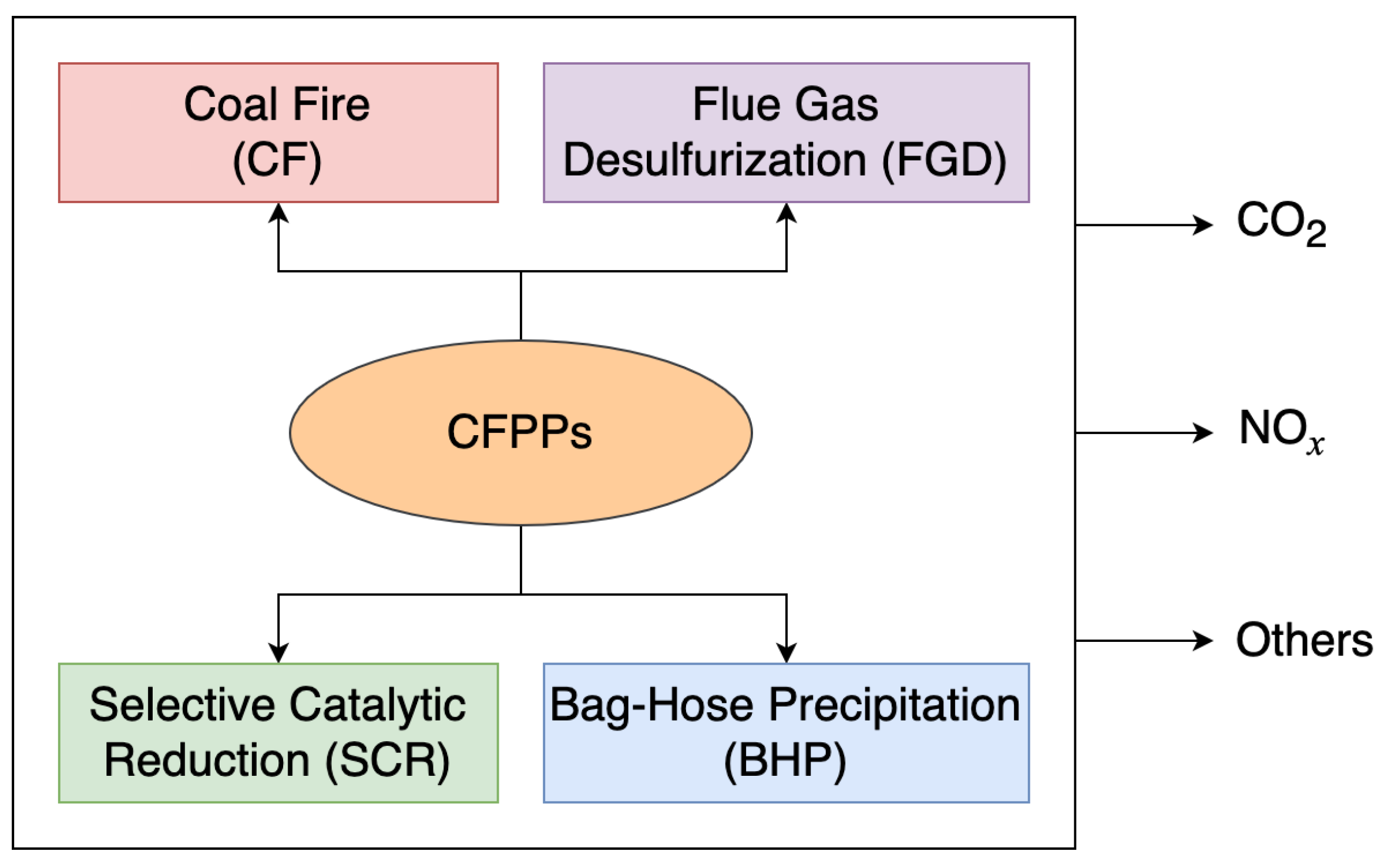
The boundary of CO emissions from CFPPs throughout the life cycle includes 5 stages: coal production, processing, transportation, coal-fired power generation, and resource utilization [8]. This paper primarily investigates the CO emissions among the stage of coal-fired power generation. Hence, the calculation was provided at the facility level of individual power plants. Considering the wide applicability and foundation of facility estimating, the boundary of CO emissions from CFPPs is described in Figure 1.
In the process of coal-fired power generation, coal consumption is the most important energy source of power plants, but also the largest direct CO emission source. The emissions mainly depend on the type of coal, combustion technology, operation conditions, maintenance quality, and the service life of the coal-fired unit. Furthermore, most of CFPPs are also equipped with flue gas desulfurization (FGD), selective catalytic reduction (SCR), and bag-hose precipitation (BHP) devices. Referring to these processes, they also produce direct CO emissions.
According to the above boundary and bottom-up approach, the CO emissions from CFPPs can be calculated as follow:
where is total CO emission from CFPPs, are CO emissions produced in the processes of coal-fired power generating units, flue gas desulfurization, selective catalytic reduction, and bag-hose precipitation, respectively. Referring to the bottom-up approach, most work is around constructing the model about these four parts. However, these works are dominated by the physical model of CFPPs and can hardly adapt to technology upgrading of CFPPs in the future. According to this problem, the following subsections introduce the basis of this research and study the key factors of .
2.2. Research Basis of This Work
CFPPs emit both direct and indirect CO emissions, where the emission factor of the direct part is closely related to the standard coal consumption for power supply. Referring to the above accounting model (1), it is obvious that coal-fired CO emissions are the primary part. To demonstrate it, this paper collected and extracted statistical data of CFPPs from related research [32,53,54,55] where the capacity of units are between 200 MW and 1000 MW. First, we analyze the emission intensity of varying stages and provide the distribution of it in Figure 2a. It shows that CO emissions of FGD, SCR, and BHP are maintained at a small level, especially, since the SCR and BHP are far smaller than 1 g/kWh. Further, Figure 2b clearly shows that the proportion of CO emissions from coal-fired plants is almost close to 99%. Hence, it is possible to infer the total CO emissions from CFPPs through power generation.
In addition, this paper presents the monthly profiles of power generation and CO emissions in Figure 3, and discovers the phenomenon that their monthly fractions of the annual amount are almost the same. Referring to Liu et al. [30], their study also supports this opinion. It means that it is possible to disaggregate long-term CO emissions (such as annual or monthly) to short-term behavior (such as monthly or weekly). It is necessary to note that the data in Figure 3 only show the monthly decomposed result. Nevertheless, shorter-period emission is easier to be affected by fluctuations in units’ load rates or any other factors. Hence, it is necessary to study all possible elements that might influence the inference near-real-time CO emissions from long-term data and net power generation.
2.3. Key Factors Contributing to the CO2 Emissions from CFPPs
2.3.1. Boiler Type
According to boiler steam parameters, such as main steam pressure and temperature, boiler types primarily are categorized into subcritical, supercritical, ultra-supercritical, and high-efficiency ultra-supercritical. Figure 4 compares the emission intensity of various boiler types and capacities.
As shown in Figure 4, for 300 MW class units, when the boilers are raised from subcritical to supercritical, the emission intensity could be decreased by ~15%. For 600 MW class units, when the boilers are enhanced from supercritical to ultra-supercritical, the emission intensity might be decreased by ~10%. For the 1000 MW class units, when the boilers are promoted from ultra-supercritical to high-efficiency ultra-supercritical, the emission intensity would be decreased by about ~5%. The primary reason is the improvement of boiler efficiency, and the generating efficiency of the unit has been promoted, too. Hence, as mentioned in Section 1.2, the model constructed on 300 MW class units might not be suitable for 600 MW or 1000 MW class units.
2.3.2. Capacity of Unit
Generally, the higher the unit capacity of the same type of boiler, the higher its power generation efficiency and the lower the standard coal consumption per unit of power generation. The results in Figure 4 preliminarily show that CO emission intensity decreases with the increase of the unit’s capacity. In addition, this paper further utilizes public and private data to analyze the distribution of emission intensity with various unit capacities. The result is shown in Figure 5.
Referring to the results shown in Figure 5, from 200 MW to 1000 MW, the average emission intensity continues to decline. It also shows that the generalization of the emission model among different CFPPs is important. Further, it also finds that the shape of the distribution of emission intensity is increasingly sharp with increasing unit’s capacity. It indicates that the larger the unit’s capacity, the less the emission intensity is affected by other factors. It is reasonable to believe from the results in Figure 5 that it is more possible to estimate emissions using net generation for larger coal-fired generating units.
2.3.3. Load Rate
The coal consumption of the power plant is the lowest when the power plant operates under the designed load level. Low-load operation will lead to an increase in coal consumption and then increase the emission intensity. Many researchers have attempted to study the relationship between unit load rate and emission intensity. Based on a large number of reliable measurements of actual CFPPs, it is shown that the higher the unit operating load, the smaller the coal consumption, and the higher the unit operating load, the higher the boiler efficiency, the lower the power supply of coal consumption [32,56]. Figure 6 clearly shows that emission intensity decreases rapidly with the increase of unit load rate, regardless of unit load capacity. Therefore, the load rate of the unit must be taken into account when estimating the CO emissions by using net power generation.
2.3.4. Coal Type
Coal is the only fuel for power generation in CFPPs. Different types of coal contain different carbon content, water content, and volatile fraction, etc. It influences boiler thermal efficiency, heat consumption rate, and plant power consumption rate deeply. Hence, the type and quality of coal directly determine the coal consumption and CO emission intensity of power generation units. The IEA estimated the average carbon emission factors for electricity generation to be 860 g/kWh, 870 g/kWh, and 1020 g/kWh for anthracite, bituminous coal, and lignite, respectively [8]. Therefore, it is not appropriate to utilize static models to estimate the CO emissions of different CFPPs.
2.3.5. Condenser Type
Currently, most CFPPs choose an air condenser, which can be divided into direct air-cooled condenser (ACC) and indirect surface condenser (ISC). ACC includes mechanical ventilation and natural ventilation according to the ventilation mode. ISC is divided into the surface condenser and mixed condenser according to the different condensers used. In fact, the type of condenser has no significant influence on the emission intensity of CFPPs, but the power consumption of every cooling equipment varies greatly, which indirectly affects the auxiliary load rate of the CFPPs, thus affecting their emission intensity. It can be found in Figure 7. Obviously, the power consumption of the cooling system is directly related to the load rate of the generation unit [32,57].
2.3.6. Auxiliary Loads
At present, using emission factors to measure the CO emissions of CFPPs is still an important solution. This approach requires, in addition to appropriate emission factors, accurate estimates of the total power generation. The total power generation is composed of net power generation and auxiliary load. Currently, the net power generation can be accurately accounted for, but there is no effective measurement for the auxiliary load. Therefore, estimating the auxiliary load is crucial for accurately measuring the CO emissions of CFPPs [32]. By studying the relationship between auxiliary load and CO emission intensity of CFPPs, Akpan [32] and She [56] found that the fraction of auxiliary load is inversely proportional to net power generation, as shown in Figure 8. Usually, the auxiliary load of a CFPP is composed of four parts: circulating pump, powder making, water pump, and fan. There are some differences between various CFPPs. Therefore, when using net power generation to estimate carbon dioxide emissions, not only the differences in the above factors but also the auxiliary load should be taken into account.
2.3.7. Summary
Through the above study, the conclusions can be drawn as follows:
- There is a strong correlation between the CO emission intensity and the load rate of the units. Therefore, it is possible to measure the short-term CO emissions of CFPPs by using the net power generation.
- When using net power generation to measure CO emissions, it is necessary to take into account the differences between the generating units of CFPPs and various operating states.
- The net power generation-based CO emission measurement model must have a strong capability of data fitting and unit adaptation.
Hence, this paper proposes a novel heterogeneous neural network and adaptation algorithm to estimate near-real-time CO emissions from CFPPs through hourly readings of power meters at the entry between CFPPs and the smart grid.
3. Method
In this section, we present our method which infers CO emissions of CFPPs through net power generation. The section introduces the framework of our proposal, the heterogeneous neural network, and its training and adaptation algorithm.
3.1. Architecture and Procedure
Figure 9 illustrates the architecture of this research work. The figure shows that the proposal consists of a deep neural network-based CO emission estimator, a regression-based CO emission simulator, and a physical variable model-based CO emission simulator. Here, the estimator poses a mathematical model between the CO emissions and the net power generation. In this way, the long-term emission can be decomposed into smaller periods. It not only approximates CO emissions by net electricity but also improves the temporal resolution of estimating CO emissions.
Further, to achieve satisfactory estimating performance, this paper designs a two-phase training strategy to eliminate the differences in the production process, unit generating efficiency, coal type, and its quality. Figure 10 is the flowchart of this training strategy. First, we create a regression-based CO emission simulator to generate a great deal of artificial data for pre-training the estimator. Obviously, the current estimator could not work for any real CFPPs, but it is well-trained to be a powerful mathematical model that can map an electricity sequence to an emission sequence. Second, this proposal designs a calibration algorithm to make an estimator adapted to any real CFPPs. In this stage, the pre-trained estimator is fed with few calibration data which contain hourly electricity and vetted daily emission. According to different situations, the vetted emission might be accounted for by bottom-up CO inventories or generated by another physical variable model-based CO emission simulator. After additional training, the estimator can be applied to monitor the CO emissions from CFPPs.
3.2. Emission Simulator
Currently, the CO emission data in high temporal resolution are still limited except for a few developed countries. For example, even though a large number of CFPPs had equipped CEMS in China, it only monitors NO, SO, and VOCs, not CO. On the other side, there are no open datasets available that report CO emissions with high temporal resolution [51], currently. Therefore, an emission simulator is important and urgent to this study. To train and validate our proposed model, this paper provides two simulators with different technical solutions for different scenarios, such as training and validation.
3.2.1. RES: Regression-Based Emission Simulator
Figure 6 shows that the CO emission intensity has a strong relationship with net power generation efficiency. Even though emission intensity is influenced by multiple factors, this paper attempts to fit the correlation between them by a nonlinear model, such as a power model, exponential model, or polynomial model, etc. By comparing their residuals, this paper chooses the cubic polynomial model to fit the relationship between emission intensity and net power generation efficiency. Furthermore, it should be mentioned that the residual of the cubic polynomial model still cannot be ignored because it is affected by many factors, especially, the demand for the power grid. Therefore, we add a normal random factor into the simulation model to ensure that the generated data are closer to the real-world data. The detailed simulation model is shown in Equation (2).
where E is the CO emission of CFPP in tons, N is the random factor, is the capacity of CFPP in MW, R is the net power generation efficiency calculated by:
where is hourly net power generation in MWh.
3.2.2. PES: Physical Variable Model-Based Emission Simulator
The physical variable model also belongs to the range of emission factor methods. However, the traditional emission factor methods and material balance methods do not consider the influence of the load rate of the power unit. Hence, they cannot be used to generate near-real-time CO emissions of CFPPs. In this section, another simulator which is based on the variable emission factor model proposed by Akpan [32] is implemented. It takes into account the re-heat architectures of CFPPs, the quality of the coal, the load conditions, and the characteristics of the boiler and cooling equipment. The detailed simulation model is provided as follows:
where is a mass fraction of carbon in the coal, is the higher heating value of coal, is the unburnt carbon loss of a boiler, is the turbine cycle heat rate at full load, is the exponential coefficient of the variable turbine cycle heat rate. and are efficiencies of the boiler and generator, respectively. is a fixed portion of the auxiliary load. can be computed by:
Since the fixed auxiliary load fraction is rarely mentioned by other studies, this paper simplifies it by a power function. By extracting the data of several CFPPs drawn from She [56] and Xu [58], this paper provides a simpler fitting model of the as following:
Different from the regression model, the , , , are randomly enough according to characteristics of CFPPs; hence, it is not necessary to add another random factor to this simulation model anymore.
3.3. Emission Estimation Network (EEN)
In order to obtain the near-real-time CO emissions from CFPPs, we include the hourly CO emission sequence and daily emissions. We proposed a model to transfer the hourly net power generation sequence to the hourly CO emission sequence, and then use the sum of them to be the daily emissions. According to the conclusion presented by [59], a time series has various types of features, and better features can be obtained by ensemble algorithms. Therefore, this paper designed a heterogeneous neural network as shown in Figure 11.
In detail, the EEN consists of AE (Auto-Encoder), MLP (MultiLayer Perceptron), and IncetionTime [60]. In addition, each network could work independently. AE is a widely applied generative model with a strong ability for denoising and data generation. With the help of its characteristics, this paper uses net power generation to generate CO emissions. Due to AE consisting of typical convolutional and transposed convolutional layers, AE is more focused on the local sequence. Hence, an MLP module is brought into EEN and it allows us to learn the global knowledge from the net power generation sequence. In addition, considering that the CO emission behavior of CFPPs has a strong local correlation in time, and the time scale is slightly different with different CFPPs, this paper introduces a revised IncetionTime module into EEN. The IncetionTime module is a ResNet-style convolution network in which every IncetionTime block owns 3 convolution paths with the different receptive field. It allows EEN to learn precise local features to improve the temporal resolution of CO emissions.
Moreover, the EEN designs an ensemble module to integrate their outputs. The following equation explains the ensemble of predictions made by all three modules:
where is the integrated CO emission sequence, R is the normalized net power generation sequence. All s are weighted to ensemble three modules’ estimation and they are all trainable.
3.4. Loss and Training
All modules of the EEN are trained in two phases:
- Independent Phase: In this phase, each neural network runs as an independent multivariate regressor. The EEN updates them to minimize the Mean Square Error (MSE), respectively:where is the estimated emissions by R, and is the L2 norm.
- Ensemble Phase: Firstly, EEN collects the outputs of every neural network independently. Then, we ensemble them through trainable weights. At this stage, the above neural networks would be frozen, and just ensemble weights should be updated. This phase can be represented by:
The EEN must be trained independently with Adam [61]. The pseudocode of the training algorithm with mini-batches is provided by Algorithm 1.
3.5. CFPP Adaptation
Referring to Figure 5 and Figure 6, the CO emission intensity is different for various CFPPs even with the same capacity. It is obvious that the estimator trained with simulation data is bound to lose effect. Therefore, it is necessary to use the data of the target CFPPs to adaptively train the pre-trained model. In the pre-training phase, Algorithm 1 optimizes the EEN based on the sequence data and takes the MSE of the sequence as the loss. Hence, to solve the lack of hourly CO emission data, this paper utilizes daily CO emission data and follows the Algorithm 1 to fine-tune EEN. The detailed steps are as follows:
- Load the pre-trained EEN.
- If there are only monthly emissions, they should be decomposed into daily emissions according to the daily fraction of the monthly net power generation as below:where and are monthly net power generation and CO emissions, respectively. and are the daily net power generation and CO emissions of the day.
- To construct the data samples, the normalized hourly net power generation is posed as input and the daily CO emissions is labeled.
- Fine-tune the pre-trained EEN following Algorithm 1 by targeting CFPP’s samples produced by the former step. In addition, the loss function of Algorithm 1 should be changed as below:where is the hourly emission, is the corresponding daily emission. and are the approximate values of CFPP’s hourly and daily in Equation (1). means expected value. When fine-tuning the EEN, the are fixed.
After the above adaptation steps, the EEN can estimate any CFPP’s hourly or daily by its net power generation. It should be mentioned that the learning rate of the adaptation stage should be far smaller than Algorithm 1.
| Algorithm 1 Mini-batch pre-training of EEN |
|
4. Experiments
In this section, we first introduce the experimental setup, and conduct experiments to answer the following questions.
- Effectiveness: How accurate are the CO emission estimation results computed by EEN and baseline methods on simulation datasets?
- Robustness: How does the robustness of EEN behave with respect to various CFPPs’ capacity levels of the test set?
- Ablation study: Does the proposed EEN contribute to a sufficiently improved estimation performance?
- Sensitivity: How does the hyperparameter of EEN influence the estimation performance?
4.1. Experiment Setting
4.1.1. Experimental Data
All training and validation data are generated by the simulator which is described in Section 3.2. To answer the above questions, this paper implements different simulation models for the training and validation stages. Firstly, this paper selected two CFPPs in each of the 300 MW, 600 MW, and 1000 MW classes for training and testing. At the same time, we collected their hourly net generation data for 1 year from CSG (China Southern Power Grid) to support the simulator to generate training and validation data. Detailed information on experimental data is introduced below:
- Training set: All data samples are generated through the Regression model mentioned in Section 3.2.1. Each daily magnitude would generate 10 samples with different random factors defined in Equation (2).
- Validation set: In order to avoid the overfitting of the EEN, the physical variable model mentioned in Section 3.2.2 was used to generate the validation dataset. For each set of electricity magnitude of CFPP, we choose different parameters randomly. Based on Akpan [32] and extensive research, the important parameters of the physical variable model are provided in Table 1.
Finally, this paper collected about 5000 training samples in total and about 300 validation samples for each simulated CFPP.
It should be mentioned that hourly electricity data are normalized by the unit’s capacity before feeding to the CO emission estimator. In addition, the emission data are also normalized by a preconfigured max value referring to each unit. Hence, the output of the estimator should be inversely normalized.
4.1.2. Baselines
The proposed EEN is compared with the following machine learning methods:
- Support Vector Regression (SVR): SVR is a popular regressor for time-series forecasting. In addition, SVR supports various kernels for different applications. The electricity magnitude and CO emissions are nonlinear. Hence, the kernel is set as Radial Basis Function(RBF) in this section, and the penalty parameter is set to 10.
- Gradient Boost Regression (GBR): GBR is one of the ensemble learning methods and uses gradient boosting with a regularized cost function. According to this study, the number of trees is set as 200, the max depth of each tree is 5, the minimum child weight equals 1, and the learning rate is configured as 0.01.
- Fully Convolution Network (FCN) [62]: FCN is proposed to perform time-series classification by Wang [62] and showed strong competitiveness. In this paper, we borrow FCN’s capability of feature learning and just change the last fully connected layer to a regressor of CO emission sequence. The outputs of the last layer are of the same shape as the input sequence and are activated by sigmoid.
- Temporal Convolutional Network (TCN) [63]: TCN brings about dilated convolutions for time series forecasting and classification and proves that dilated convolutions outperform RNNs in terms of both efficiency and predictive performance. In this paper, the TCN equipped two dilated convolutional blocks. Each block contains two 1D convolutional layers with a dilation parameter of (1,2,4,8) and each convolutional layer consists of 64 filters. The output layer is the same as FCN.
- LSTM: It is a stack of an LSTM layer and a fully connected layer. The hidden size of the LSTM layer is 8, and the output layer is the same as the last layer of FCN.
The above competitor list includes both traditional and deep approaches. In addition, these baseline methods employ different learning strategies. Hence, the above baseline list can well represent the competing performance of this research. The KNN, SVR, and GBR are based on scikit-learn [64]. In addition, all of the deep neural networks are developed on Keras.
4.1.3. Configuration
In this paper, the primary parameters of EEN are shown in Figure 11. Our proposed EEN and all baseline models are optimized with the Adam optimizer, and its learning rate is fixed as for pre-train and for adaptation. The total number of epochs is 100 with proper early stopping. We set the baseline methods as recommended, and the batch size is 100.
4.1.4. Evaluation Metrics and Computing Infrastructure
In order to compare with the above methods, the Mean Absolute Percentage Error (MAPE) can be applied to evaluate the performance of our proposal and baselines. Since the performance of hourly and daily estimations are both important in this paper, the detailed metrics are defined as follows:
where and are the MAPE of hourly and daily estimation, respectively. and are labeled and estimated hourly CO emissions, and is the absolute value function. n is the number of estimations.
4.2. Results
4.2.1. Results and Analysis
Table 2 and Table 3 summarize the daily/hourly CO emission estimation results of all the methods on simulated CFPPs. Since the KNN, SVR, and GBR could not support daily and hourly estimating simultaneously, this paper collects their daily and hourly estimation results for independent models. Hence, they are not suitable for deep learning-based methods. The best results are highlighted in boldface. It should be mentioned that, unless otherwise noted below, the experimental results are based on 30 adaptation samples.
Daily CO2 Emission Estimating
Under this setting, KNN, SVR and GBR attain estimations as a single variable over the time series, while the remaining deep learning methods always estimate hourly CO emissions and account them as daily emissions. From Table 2, it can be observed that: (1) The proposed model EEN significantly improves the inference performance across all simulated CFPPs, and their estimate error keeps stable for various CFPPs, which demonstrates the success of EEN in enhancing the estimation capacity in the problem of monitoring CO emissions of CFPPs. (2) Generally, deep learning-based methods are better than traditional machine learning methods, because the deep neural network has a strong data fitting ability. (3) The proposed EEN is outperforms TCN, FCN and LSTM on MAPE by decreasing 40–60% in average. It shows that our method is more stable and powerful.
Hourly CO2 Emission Estimating
Within this setting, KNN, SVR, and GBR are inappropriate and require to be changed from univariate prediction to multivariate one by redesigning the models. On the contrary, our proposed EEN is easy to adapt to the daily and hourly situation without any adjusting to the model. From Table 3, it can be observed that: (1) the proposed model EEN greatly outperforms other methods, and the findings 1 and 2 in the daily settings still hold for the hourly CO emissions. (2) The EEN model shows better results than baselines, and the MAPE decreases about 20–46% on average. Compared with the daily results, the overwhelming performance is reduced, and such phenomena can be caused by the uncertainty of power demand in a short time period. It is beyond the scope of this paper, and we will explore it in future work.
In addition, this paper uses an exact sample to show that our EEN model is powerful to predict the details of CO emission behavior in Figure 12 and Figure 13. According to this setting, this paper utilizes Akpan [32] as ground truth and compares the effectiveness of all methods on the same example. The most related work shows acceptable results. TCN and TCN have a good performance on daily emissions, but it is easy to miss details when estimating hourly emissions. There are similar problems with other approaches. Our proposed model EEN shows significantly better results than other methods for both daily and hourly CO emission estimating.
4.2.2. Ablation Study
This subsection conducts additional experiments with ablation consideration and demonstrates how well EEN works.
Performance of Ensembling
In this study, we compare the MAPE of our adaptive ensembling and average ensembling in Figure 14. Firstly, due to EEN consisting of heterogeneous neural networks, it allows EEN to capture various features and fit the relationship between net power generation and CO emissions of CFPPs. Comparing the results of Figure 14 and Table 2 and Table 3, average ensembling is still better than a single model. It demonstrates that the EEN is competent for CO emission estimation. Second, due to the ensembling weights of EEN being learnable, EEN could provide better integration of heterogeneous neural networks. Compared to average ensembling, EEN achieved about 20% and 7% improvement on daily and hourly MAPE, respectively.
Performance of Adaptation
Our approach presents a CFPP adaptation mechanism to help EEN which is pre-trained by simulated data to different CFPPs. In this study, we validate the effectiveness of this mechanism. In Table 4, we compare the daily and hourly MAPE before and after adaptation. In this setting, this paper still utilizes 30 samples of target CFPPs to finish adaptation training. Referring to the results of Table 4, it can be observed that the CFPP adaptation mechanism improves the performance of EEN on daily and hourly MAPE about 69% and 27% on average, respectively.
Robustness of EEN
Referring to the limit of effective samples mentioned in Section 3.2, it is necessary to validate the robustness of EEN for fewer samples. In this experiment, we study the performance of EEN for varying adaptation samples. From the results of Figure 15, it can be observed that the EEN could still keep competitive performance even with just 10 adaptation samples. Especially, the difference between daily and hourly MAPE are both limited within 0.4%. However, it could also be found that more adaptation samples would acquire better performance.
4.2.3. Uncertainties
This paper estimated the uncertainty of the fit performance of EEN. We estimated uncertainties of daily and hourly MAPE of EEN for individually simulated CFPP. In this section, the original and unaveraged estimated error and the Absolute Percentage Error (APE) are used to discuss the uncertainty of EEN. In detail, APE is computed as below:
where is the APE of the time unit, day or hour. and might be the labeled and estimated daily or hourly CO emissions.
Uncertainty of Daily CO Emission Estimation
This paper collects all APE of every day and every CFPPs and does a statistics of them, respectively. From Figure 16, it can be found that APE of EEN is mostly located between 0% and 3%. For each CFPP, the standard deviation of daily APE is around 0.9%. Only a few extreme cases are beyond 4%, but still limited within 8%.
Uncertainty of Hourly CO2 Emission Estimation
In this study, we separately analyzed the distribution of hourly APE across different days. From Figure 17, it can be observed that hourly APE is distributed within a range of compared to the hourly MAPE. Even though the hourly APE between 0–6 A.M. is higher than that of other time periods, the standard deviation remained stable. Hence, it can be concluded that the uncertainty of hourly CO emission estimation is limited.
Uncertainty of CO2 Emission Estimation at Different Load Conditions
In this study, we continue to discuss the uncertainty of hourly CO emissions according to different load rates. From Figure 18, the load rate of CFPPs would affect the MAPE of EEN. When the load rate is smaller than 50%, the hourly CO emissions are more easily affected by boiler efficiency and auxiliary loads, and the uncertainty of CO emission estimation is greater. With the increase in load rate, the uncertainty is improved obviously. Especially, the standard deviation of hourly APE would be decreased by about 1% when the load rate is over 60%. According to the results of Figure 18, which has a commonplace with Figure 17, the hourly APE is higher in the period of 0–6 A.M. because the load rate of CFPPs in such time period is lower.
4.3. Summary of Experiments
First, EEN outperforms other baseline machine learning and deep learning algorithms on the same dataset. Not only the MAPE of CO emissions but also the stability and uncertainty, the experimental results all show that EEN has better performance and robustness.
Second, in Table 2, the of EEN is only about 1%. It shows that the performance of EEN is close to Akpan [32]. However, besides net power generation and capacity of the unit, Akpan [32] requires a series of parameters, such as the mass fraction of carbon in the coal, heating value of coal, turbine cycle heat rate at full load, exponential coefficient of the variable turbine cycle heat rate, etc. These parameters are not only difficult to collect, but it is also hard to determine their exact values. Hence, our approach is easier to apply.
Finally, this paper utilizes emissions estimated by the Akpan [32] model as the ground truth to analyze the uncertainty of EEN. From the experimental results, the uncertainties are limited to 10%. However, the uncertainties of the methods proposed by Liu [4] and Hu [41] are both more than 20%. Compared to the current EEN, they are more convenient and generalizable because they both use OCO-2 data.
5. Conclusions
Overall, this paper provides the following contributions:
- This paper provides the quantitative relationship between CO emissions from CFPPs and all primary elements. Through analyzing the data extracted from a wide range of related research, we found that there is an inherent mathematical relationship between the net power generation and the emission intensity. Further, the proportion of emissions produced by auxiliary equipment of CFPPs is very small and all of them are related to an auxiliary power load. This conclusion provides the motivation for our research and guides us to design EEN and related algorithms. At last, it could be found that the emission intensity is different from CFPPs.
- This paper provides a novel and purely data-driven approach to estimate near-real-time CO emissions from CFPPs by net power generation. We introduce deep learning into estimating emissions from CFPPs, and our proposed EEN is a deep assembling model based on heterogeneous neural networks. The experimental results show that EEN owns outperforming data fitting and generalization capabilities. Furthermore, it is worth pointing out that our proposed EEN only requires the hourly readings of the power meters on the link between CFPPs and the smart grid as net power generation. Hence, it is an easy solution to implement.
- This paper provides a novel training algorithm so that our proposed EEN could be adapted to any CFPPs by a few realistic datasets. Due to the limitation of real and well-vetted data, we present a two-phase training algorithm: pre-train and adaptation. First, we use a large number of artificial data generated by a regression model-based simulator to pre-train our proposed EEN. Then, we utilize a few datasets collected from the target CFPP to finish the adaptation of EEN. This strategy allows us to utilize less realistic data to adapt to any CFPPs at the stage of application. This further reduces the cost of the application and improves the implementability.
In this study, a novel data-driven framework for monitoring CO emissions from CFPPs in near-real-time is presented to avoid installing expensive and complicated CEMS. Firstly, we investigate all possible elements of CO emissions from CFPPs. We found that the net power generation is strongly related to the emission intensity, and the emission intensity is different from CFPPs. Next, we propose a deep ensembling model based on heterogeneous neural networks with powerful data fitting and generalization capabilities. Then, due to the limitation of real and well-labeled data, we present a two-phase training algorithm: pre-train and adaptation. We use a large number of artificial datasets generated by the simulator to pre-train our proposed EEN. We allow to utilize fewer datasets of the target CFPP to finish calibration at the stage of application. At last, the experimental results show that our scheme outperforms all baselines.
We found that it is feasible to infer CO emissions from the net power generation of CFPPs, but limitations of the current real-world data only allow us to verify our method on the simulator. Looking forward, we anticipate that these limitations will diminish for more CFPPs to place greater emphasis on data collection and analysis so that our proposed EEN could be adapted to more CFPPS. Therefore, future work will be to validate and optimize our method to the real CFPPs equipped with CEMS or to hold perfectly vetted datasets.
Author Contributions
Conceptualization, S.Z.; methodology, S.Z. and H.H.; validation, L.Z.; resources, W.Z.; writing—original draft preparation, S.Z. and H.H.; writing—review and editing, F.W.; supervision, S.Z. All authors have read and agreed to the published version of the manuscript.
Funding
This research was funded by Digital Grid Research Institute, China Southern Power Grid, and Guangdong Provincial Key Laboratory of Digital Grid Technology, grant number 670000KK52210037.
Data Availability Statement
Not applicable.
Conflicts of Interest
The authors declare no conflict of interest.
References
- Stocker, T.F.; Qin, D.; Plattner, G.-K.; Tignor, M.; Allen, S.K.; Boschung, J.; Nauels, A.; Xia, Y.; Bex, V.; Midgley, P.M. Climate Change 2013: The Physical Science Basis, Working Group I Contribution to the Fifth Assessment Report of the Intergovernmental Panel on Climate Change; Cambridge University Press: Cambridge, UK; New York, NY, USA, 2013; ISBN 978-1-107-66182-0. [Google Scholar]
- Masson-Delmotte, V.; Zhai, P.; Pirani, A.; Connors, S.L.; Péan, C.; Berger, S.; Caud, N.; Chen, Y.; Goldfarb, L.; Gomis, M.I.; et al. Climate Change 2021: The Physical Science Basis. Contribution of Working Group I to the Sixth Assessment Report of the Intergovernmental Panel on Climate Change; Cambridge University Press: Cambridge, UK, 2021. [Google Scholar] [CrossRef]
- Janssens-Maenhout, G.; Crippa, M.; Guizzardi, D.; Muntean, M.; Schaaf, E.; Dentener, F.; Bergamaschi, P.; Pagliari, V.; Olivier, J.G.J.; Peters, J.A.H.W.; et al. EDGAR v4.3.2 Global Atlas of the three major greenhouse gas emissions for the period 1970–2012. Earth Syst. Sci. Data 2019, 11, 959–1002. [Google Scholar] [CrossRef]
- Liu, F.; Duncan, B.N.; Krotkov, N.A.; Lamsal, L.N.; Beirle, S.; Griffin, D.; McLinden, C.A.; Goldberg, D.L.; Lu, Z. A methodology to constrain carbon dioxide emissions from coal-fired power plants using satellite observations of co-emitted nitrogen dioxide. Atmos. Chem. Phys. 2020, 20, 99–116. [Google Scholar] [CrossRef]
- Yang, Z.; Dou, X.; Jiang, Y.; Luo, P.; Ding, Y.; Zhang, B.; Tang, X. Tracking the CO2 Emissions of China’s Coal Production via Global Supply Chains. Energies 2022, 15, 5934. [Google Scholar] [CrossRef]
- Shindell, D.; Faluvegi, G. The net climate impact of coal-fired power plant emissions. Atmos. Chem. Phys. 2010, 10, 3247–3260. [Google Scholar] [CrossRef]
- Xie, H.P.; Wu, L.X.; Zheng, D.Z. Prediction on the energy consumption and coal demand of China in 2025. J. China Coal Soc. 2019, 44, 1949–1960. [Google Scholar] [CrossRef]
- Wang, N.; Ren, Y.; Zhu, T.; Meng, F.; Wen, Z.; Liu, G. Life cycle carbon emission modelling of coal-fired power: Chinese case. Energy 2018, 162, 841–852. [Google Scholar] [CrossRef]
- Hubacek, K.; Baiocchi, G.; Feng, K.S.; Patwardhan, A. Poverty eradication in a carbon constrained world. Nat. Commun. 2017, 8, 912. [Google Scholar] [CrossRef] [PubMed]
- Wiedenhofer, D.; Guan, D.B.; Liu, Z.; Meng, J.; Zhang, N.; Wei, Y.M. Unequal household carbon footprints in China. Nat. Clim. Chang. 2016, 7, 75–80. [Google Scholar] [CrossRef]
- Zhao, J.; Yang, K. Analysis of CO2 Abatement Cost of Solar Energy Integration in a Solar-Aided Coal-Fired Power Generation System in China. Sustainability 2020, 12, 6587. [Google Scholar] [CrossRef]
- Ashizawa, M.; Otaka, M.; Yamamoto, H.; Akisawa, A. CO2 Emissions and Economy of Co-Firing Carbonized Wood Pellets at Coal-Fired Power Plants: The Case of Overseas Production of Pellets and Use in Japan. Energies 2022, 15, 1770. [Google Scholar] [CrossRef]
- Liu, X.; Gao, X.; Wu, X.; Yu, W.; Chen, L.; Ni, R.; Zhao, Y.; Duan, H.; Zhao, F.; Chen, L.; et al. Updated hourly emissions factors for Chinese power plants showing the impact of widespread ultralow emissions technology deployment. Environ. Sci. Technol. 2019, 53, 2570–2578. [Google Scholar] [CrossRef] [PubMed]
- Wu, Y.J.; Xu, Z.F.; Li, Z. Lifecycle analysis of coal-fired power plants with ccs in china. Energy Procedia 2014, 63, 7444–7451. [Google Scholar]
- Lee, B.J.; Lee, J.I.; Yun, S.Y.; Hwang, B.G.; Lim, C.-S.; Park, Y.-K. Methodology to Calculate the CO2 Emission Reduction at the Coal-Fired Power Plant: CO2 Capture and Utilization Applying Technology of Mineral Carbonation. Sustainability 2020, 12, 7402. [Google Scholar] [CrossRef]
- Zhou, K.; Yang, S.; Shen, C.; Ding, S.; Sun, C. Energy conservation and emission reduction of China’s electric power industry. Renew. Sustain. Energy Rev. 2015, 45, 10–19. [Google Scholar] [CrossRef]
- Wang, L.; Jang, C.; Yang, Z.; Kai, W.; Qiang, Z.; Streets, D.; Fu, J.; Yu, L.; Schreifels, J.; He, K. Assessment of air quality benefits from national air pollution control policies in China. Part II: Evaluation of air quality predictions and air quality benefits assessment. Atmos. Environ. 2010, 44, 3449–3457. [Google Scholar] [CrossRef]
- Liu, S.; Hua, S.; Wang, K.; Qiu, P.; Liu, H.; Wu, B.; Shao, P.; Liu, X.; Wu, Y.; Xue, Y. Spatial-temporal variation characteristics of air pollution in Henan of China: Localized emission inventory, WRF/Chem simulations and potential source contribution analysis. Sci. Total Environ. 2018, 624, 396–406. [Google Scholar] [CrossRef] [PubMed]
- Alnaim, A.; Sun, Z.; Tong, D. Evaluating Machine Learning and Remote Sensing in Monitoring NO2 Emission of Power Plants. Remote Sens. 2022, 14, 729. [Google Scholar] [CrossRef]
- Gómez, D.R.; Watterson, J.D. 2006 IPCC Guidelines for National Greenhouse Gas Inventories; U.S. Department of Energy Office of Scientific and Technical Information: Oak Ridge, TN, USA, 2006; Volume 2.
- Myeong, J.E.C.; Sa, S.J.; Kim, J.W.; Jeong, J.S. Greenhouse gas emission factor development for coal-fired power plants in Korea. Appl. Energy 2010, 87, 205–210. [Google Scholar]
- Mittal, M.L.; Sharma, C.; Singh, R. Estimates of emissions from coal fired thermal power plants in India. In Proceedings of the International Emission Inventory Conference, Tampa, FL, USA, 13–16 August 2012; pp. 13–16. [Google Scholar]
- Gutierrez-Martín, F.; Da Silva-Alvarez, R.A.; Montoro-Pintado, P. Effects of wind intermittency on reduction of CO2 emissions: The case of the Spanish power system. Energy 2013, 61, 108–117. [Google Scholar] [CrossRef]
- Oates, D.L.; Jaramillo, P. Production cost and air emissions impacts of coal cycling in power systems with large-scale wind penetration. Environ. Res. Lett. 2013, 8, 024022. [Google Scholar] [CrossRef]
- Yu, S.; Wei, Y.M.; Guo, H.; Ding, L. Carbon emission coefficient measurement of the coal-to-power energy chain in China. Appl. Energy 2014, 114, 290–300. [Google Scholar] [CrossRef]
- Wierzbowski, M.; Lyzwa, W.; Musial, I. MILP model for long-term energy mix planning with consideration of power system reserves. Appl. Energy 2016, 169, 93–111. [Google Scholar] [CrossRef]
- Gonzalez-salazar, M.A.; Kirsten, T.; Prchlik, L. Review of the operational flexibility and emissions of gas- and coal- fired power plants in a future with growing renewables. Renew. Sustain. Energy Rev. 2018, 82, 497–513. [Google Scholar] [CrossRef]
- Alfredo, V.; Vladimir, F. Evaluating and forecasting direct carbon emissions of electricity production: A case study for South East Europe. Energy Sources Part B Econ. Plan. Policy 2022, 17, 2037028. [Google Scholar] [CrossRef]
- Lin, J.-T.; McElroy, M.B.; Boersma, K.F. Constraint of anthropogenic NOx emissions in China from different sectors: A new methodology using multiple satellite retrievals. Atmos. Chem. Phys. 2010, 10, 63–78. [Google Scholar] [CrossRef]
- Liu, F.; Zhang, Q.; Tong, D.; Zheng, B.; Li, M.; Huo, H.; He, K.B. High-resolution inventory of technologies, activities and emissions of coal-fired power plants in China from 1990 to 2010. Atmos. Chem. Phys. 2015, 15, 13299–13317. [Google Scholar] [CrossRef]
- Chen, X.; Liu, Q.; Sheng, T.; Li, F.; Xu, Z.; Han, D.; Zhang, X.; Huang, X.; Fu, Q.; Cheng, J. A high temporal-spatial emission inventory and updated emission factors for coal-fired power plants in Shanghai, China. Sci. Total Environ. 2019, 688, 94–102. [Google Scholar] [CrossRef]
- Akpan, P.U.; Fuls, W.F. Cycling of coal fired power plants: A generic CO2 emissions factor model for predicting CO2 emissions. Energy 2021, 214, 119026. [Google Scholar] [CrossRef]
- U.S. Environmental Protection Agency. Plain English Guide to the Part 75 Rule; U.S. Environmental Protection Agency: Washington, DC, USA, 2005.
- Burrows, J.P.; Hölzle, E.; Goede, A.P.H.; Visser, H.; Fricke, W. SCIAMACHY—Scanning imaging absorption spectrometer for atmospheric chartography. Acta Astronaut. 1995, 35, 445–451. [Google Scholar] [CrossRef]
- Yokota, T.; Yoshida, Y.; Eguchi, N.; Ota, Y.; Tanaka, T.; Watanabe, H.; Maksyutov, S. Global Concentrations of CO2 and CH4 Retrieved from GOSAT: First Preliminary Results. SOLA 2009, 5, 160–163. [Google Scholar] [CrossRef]
- Crisp, D. Measuring atmospheric carbon dioxide from space with the Orbiting Carbon Observatory-2 (OCO-2). Proc. SPIE 2015, 9607, 960702. [Google Scholar] [CrossRef]
- Konovalov, I.B.; Berezin, E.V.; Ciais, P.; Broquet, G.; Zhuravlev, R.V.; Janssens-Maenhout, G. Estimation of fossil-fuel CO2 emissions using satellite measurements of “proxy” species. Atmos. Chem. Phys. 2016, 16, 13509–13540. [Google Scholar] [CrossRef]
- Nassar, R.; Hill, T.G.; McLinden, C.A.; Wunch, D.; Jones, D.B.A.; Crisp, D. Quantifying CO2 Emissions from Individual Power Plants From Space. Geophys. Res. Lett. 2017, 44, 10045–10053. [Google Scholar] [CrossRef]
- Reuter, M.; Buchwitz, M.; Schneising, O.; Krautwurst, S.; O’Dell, C.W.; Richter, A.; Bovensmann, H.; Burrows, J.P. Towards monitoring localized CO2 emissions from space: Co-located regional CO2 and NO2 enhancements observed by the OCO-2 and S5P satellites. Atmos. Chem. Phys. 2019, 19, 9371–9383. [Google Scholar] [CrossRef]
- Wang, C.; Wang, T.; Wang, P.; Rakitin, V. Comparison and Validation of TROPOMI and OMI NO2 Observations over China. Atmosphere 2020, 11, 636. [Google Scholar] [CrossRef]
- Hu, Y.; Shi, Y. Estimating CO2 Emissions from Large Scale Coal-Fired Power Plants Using OCO-2 Observations and Emission Inventories. Atmosphere 2021, 12, 811. [Google Scholar] [CrossRef]
- Ackerman, K.V.; Sundquist, E.T. Comparison of two US power-plant carbon dioxide emissions data sets. Environ. Sci. Technol. 2008, 42, 5688–5693. [Google Scholar] [CrossRef] [PubMed]
- Russakovsky, O.; Deng, J.; Su, H.; Krause, J.; Satheesh, S.; Ma, S.; Huang, Z.; Karpathy, A.; Khosla, A.; Bernstein, M.; et al. ImageNet Large Scale Visual Recognition Challenge. Int. J. Comput. Vis. 2015, 115, 211–252. [Google Scholar] [CrossRef]
- Deng, L.; Hinton, G.; Kingsbury, B. New types of deep neural network learning for speech recognition and related applications: An overview. In Proceedings of the 2013 IEEE International Conference on Acoustics, Speech and Signal Processing, Vancouver, BC, Canada, 26–31 May 2013; pp. 8599–8603. [Google Scholar]
- Wu, Y.; Schuster, M.; Chen, Z.; Le, Q.V.; Norouzi, M.; Macherey, W.; Krikun, M.; Cao, Y.; Gao, Q.; Macherey, K.; et al. Googles Neural Machine Translation System: Bridging the Gap between Human and Machine Translation. arXiv 2016, arXiv:1609.08144. [Google Scholar]
- Sun, W.; Wang, C.; Zhang, C. Factor analysis and forecasting of CO2 emissions in Hebei, using extreme learning machine based on particle swarm optimization. J. Clean. Prod. 2017, 162, 1095–1101. [Google Scholar] [CrossRef]
- Zhao, H.; Huang, G.; Yan, N. Forecasting Energy-Related CO2 Emissions Employing a Novel SSA-LSSVM Model: Considering Structural Factors in China. Energies 2018, 11, 781. [Google Scholar] [CrossRef]
- Amarpuri, L.; Yadav, N.; Kumar, G.; Agrawal, S. Prediction of CO2 emissions using deep learning hybrid approach: A Case Study in Indian Context. In Proceedings of the IEEE Twelfth International Conference on Contemporary Computing (IC3), Noida, India, 8–10 August 2019; pp. 1–6. [Google Scholar]
- Nam, K.; Hwangbo, S.; Yoo, C. A deep learning-based forecasting model for renewable energy scenarios to guide sustainable energy policy: A case study of Korea. Renew. Sustain. Energy Rev. 2020, 122, 109725. [Google Scholar] [CrossRef]
- Huang, H.; Wu, X.; Cheng, X. The Prediction of Carbon Emission Information in Yangtze River Economic Zone by Deep Learning. Land 2021, 10, 1380. [Google Scholar] [CrossRef]
- Alfaseeh, L.; Tu, R.; Farooq, B.; Hatzopoulou, M. Greenhouse gas emission prediction on road network using deep sequence learning. Transp. Res. Part D Transp. Environ. 2020, 88, 102593. [Google Scholar] [CrossRef]
- Singh, M.; Dubey, R. Deep Learning Model Based CO2 Emissions Prediction using Vehicle Telematics Sensors Data. IEEE Trans. Intell. Veh. 2021, 8, 768–777. [Google Scholar] [CrossRef]
- Long, Y. Study on Calculation Model and Method of Carbon Dioxide Emissions for Coal-fired Power Plant. Master’s Thesis, College of Power Engineering of Chongqing University, Chongqing, China, 2016. (In Chinese). [Google Scholar]
- Suo, X.L.; Sheng, J.G.; Wang, P.H.; Liu, J.T. CO2 Emissions Calculation and Analysis of Carbon Emissions of Coal-fired Generating Unit. Power Syst. Eng. 2018, 34, 13–16. (In Chinese) [Google Scholar]
- Li, J.; Yu, H.Q.; Chen, R. Analysis and application of calculating method for CO2 emission intensity per unit of electricity generation in coal-fired power plants. Chin. J. Environ. Eng. 2015, 9, 3419–3425. (In Chinese) [Google Scholar]
- She, Y.Y.; Gao, P.D.; Zhang, H.C.; Liu, H.G.; Shao, Y.H.; Hu, D.W.; Zhou, K. Economy study for units running at full load burning coals with different calorific values. Therm. Power Gener. 2021, 50, 63–69. (In Chinese) [Google Scholar]
- Ma, X.L.; Wang, X.F.; Sun, X.J.; Shi, J.; Chen, J.P.; Dang, L.C. Influence factors of carbon emission intensity of coal-fired power units. Therm. Power Gener. 2022, 51, 190–195. (In Chinese) [Google Scholar]
- Xu, Q. Study on Optimization and Supervision Analysis of Auxiliary Power Ratio in the 600 MW Units. Master’s Thesis, School of Electronic Information and Electrical Engineering of Shanghai JiaoTong University, Shanghai, China, 2016. (In Chinese). [Google Scholar] [CrossRef]
- Lines, J.; Taylor, S.; Bagnall, A. HIVE-COTE: The Hierarchical Vote Collective of Transformation-Based Ensembles for Time Series Classification. In Proceedings of the IEEE 16th International Conference on Data Mining (ICDM), Barcelona, Spain, 12–15 December 2016; pp. 1041–1046. [Google Scholar] [CrossRef]
- Fawaz, H.; Lucas, B.; Forestier, G.; Pelletier, C.; Schmidt, D.F.; Weber, J.; Webb, G.I.; Idoumghar, L.; Muller, P.A.; Petitjean, F. InceptionTime: Finding AlexNet for time series classification. Data Min. Knowl. Discov. 2020, 34, 1936–1962. [Google Scholar] [CrossRef]
- Kingma, D.; Ba, J. Adam: A Method for Stochastic Optimization. arXiv 2014, arXiv:1412.6980. [Google Scholar]
- Wang, Z.; Yan, W.; Oates, T. Time series classification from scratch with deep neural networks: A strong baseline. In Proceedings of the 2017 International Joint Conference on Neural Networks, Anchorage, AK, USA, 14–19 May 2017; pp. 1578–1585. [Google Scholar]
- Bai, S.; Kolter, J.Z.; Koltun, V. An Empirical Evaluation of Generic Convolutional and Recurrent Networks for Sequence Modeling. arXiv 2018, arXiv:1803.01271. [Google Scholar]
- Pedregosa, F.; Varoquaux, G.; Gramfort, A.; Michel, V.; Thirion, B.; Grisel, O.; Blondel, M.; Prettenhofer, P.; Weiss, R.; Dubourg, V.; et al. Scikit-learn: Machine learning in Python. J. Mach. Learn. Res. 2011, 12, 2825–2830. [Google Scholar]
Figure 1.
CO emission boundary of coal-fired power plants.

Figure 2.
(a) Distribution of CO emission intensity in varying stages. (b) Percentage of emissions from coal-fired units.
Figure 2.
(a) Distribution of CO emission intensity in varying stages. (b) Percentage of emissions from coal-fired units.

Figure 3.
Monthly profiles of thermal power generation and coal-fired power-plant CO emissions.

Figure 4.
Emission intensity for different boiler types.

Figure 5.
Distribution of CO emission intensity for various unit capacities.

Figure 6.
The relationship between CO emission intensity and power unit generation efficiency.

Figure 7.
Comparison of the emission intensity of different condensers.

Figure 8.
The relationship between auxiliary load fraction and efficiency of net generation [32,56].

Figure 9.
The architecture of the proposal.

Figure 10.
Flowchart of this proposal.

Figure 11.
The architecture of Emission Estimation Network.

Figure 12.
Comparison of estimated hourly CO emissions. (a–f) compare the estimated hourly CO emissions between Akpan and EEN, FCN, LSTM, TCN, SVR, and GBR, respectively.
Figure 12.
Comparison of estimated hourly CO emissions. (a–f) compare the estimated hourly CO emissions between Akpan and EEN, FCN, LSTM, TCN, SVR, and GBR, respectively.

Figure 13.
Comparison of estimated daily CO emissions. (a–f) compare the estimated daily CO emissions between Akpan and EEN, FCN, LSTM, TCN, SVR, and GBR, respectively.
Figure 13.
Comparison of estimated daily CO emissions. (a–f) compare the estimated daily CO emissions between Akpan and EEN, FCN, LSTM, TCN, SVR, and GBR, respectively.

Figure 14.
Ablation study of ensembling: Comparing the performance of different ensemble methods on hourly and daily CO emission estimation. (a) The MAPE of daily emission estimation; (b) the MAPE of hourly emission estimation.
Figure 14.
Ablation study of ensembling: Comparing the performance of different ensemble methods on hourly and daily CO emission estimation. (a) The MAPE of daily emission estimation; (b) the MAPE of hourly emission estimation.

Figure 15.
Study on the influence of the varying number of adaptation samples on EEN. (a) The MAPE of daily emission estimation; (b) the MAPE of hourly emission estimation.
Figure 15.
Study on the influence of the varying number of adaptation samples on EEN. (a) The MAPE of daily emission estimation; (b) the MAPE of hourly emission estimation.

Figure 16.
Analysis of uncertainty of EEN according to estimated daily CO emissions.

Figure 17.
Analysis of the uncertainty of EEN according to estimated hourly CO emissions at different hours.
Figure 17.
Analysis of the uncertainty of EEN according to estimated hourly CO emissions at different hours.

Figure 18.
Analysis of the uncertainty of EEN according to estimated hourly CO emissions at varying load rates.
Figure 18.
Analysis of the uncertainty of EEN according to estimated hourly CO emissions at varying load rates.


Table 1.
The range of simulation parameters used in the physical variable model.
| Simulated CFPP | Capacity (MW) | Range of | Range of | ||
|---|---|---|---|---|---|
| 1 | 300 | 9016.5 | 0.1087 | [0.56, 0.59] | [21, 22] |
| 2 | 300 | 8623.8 | 0.1127 | [0.56, 0.59] | [21, 22] |
| 3 | 600 | 7962.3 | 0.0624 | [0.58, 0.60] | [22, 23] |
| 4 | 600 | 7548.6 | 0.0716 | [0.58, 0.60] | [22, 23] |
| 5 | 1000 | 7396.4 | 0.0542 | [0.59, 0.61] | [23, 24] |
| 6 | 1000 | 7062.8 | 0.0602 | [0.59, 0.61] | [23, 24] |
Here, and HHV are selected randomly within the corresponding range, respectively.
Table 2.
MAPE of daily CO emissions.
| EEN | KNN | SVR | GBR | TCN | FCN | LSTM | |
|---|---|---|---|---|---|---|---|
| 300 MW-1 | 1.03 | 2.54 | 2.23 | 1.86 | 1.95 | 2.02 | 1.83 |
| 300 MW-2 | 0.98 | 3.01 | 2.45 | 2.25 | 1.89 | 1.74 | 1.72 |
| 600 MW-1 | 1.37 | 3.42 | 4.72 | 2.32 | 2.47 | 2.50 | 2.20 |
| 600 MW-2 | 1.07 | 3.63 | 3.63 | 2.42 | 2.18 | 2.61 | 1.93 |
| 1000 MW-1 | 1.11 | 2.98 | 3.12 | 2.78 | 2.10 | 2.73 | 2.07 |
| 1000 MW-2 | 1.28 | 3.11 | 4.35 | 2.57 | 2.32 | 2.81 | 2.18 |
Table 3.
MAPE of hourly CO emissions.
| EEN | KNN | SVR | GBR | TCN | FCN | LSTM | |
|---|---|---|---|---|---|---|---|
| 300 MW-1 | 5.18 | 8.59 | 9.05 | 7.09 | 6.45 | 6.95 | 8.19 |
| 300 MW-2 | 5.33 | 9.06 | 9.08 | 7.57 | 6.55 | 6.65 | 8.58 |
| 600 MW-1 | 5.29 | 9.37 | 10.09 | 7.40 | 6.74 | 7.29 | 8.67 |
| 600 MW-2 | 5.36 | 9.33 | 9.75 | 7.41 | 6.78 | 7.49 | 8.69 |
| 1000 MW-1 | 5.32 | 8.97 | 9.16 | 7.81 | 6.73 | 7.48 | 8.57 |
| 1000 MW-2 | 5.48 | 8.82 | 10.18 | 7.76 | 6.58 | 7.34 | 8.65 |
Table 4.
Comparing the MAPE of EEN before and after adaptation about daily and hourly CO emission estimation.
Table 4.
Comparing the MAPE of EEN before and after adaptation about daily and hourly CO emission estimation.
| Before Adaptation | After Adaptation | Before Adaptation | After Adaptation | |
| 300 MW-1 | 6.11 | 5.18 | 2.55 | 1.03 |
| 300 MW-2 | 6.09 | 5.33 | 2.51 | 0.98 |
| 600 MW-1 | 8.67 | 5.29 | 4.88 | 1.37 |
| 600 MW-2 | 7.94 | 5.36 | 4.71 | 1.07 |
| 1000 MW-1 | 7.89 | 5.32 | 4.25 | 1.11 |
| 1000 MW-2 | 8.13 | 5.48 | 4.72 | 1.28 |
Disclaimer/Publisher’s Note: The statements, opinions and data contained in all publications are solely those of the individual author(s) and contributor(s) and not of MDPI and/or the editor(s). MDPI and/or the editor(s) disclaim responsibility for any injury to people or property resulting from any ideas, methods, instructions or products referred to in the content. |
© 2023 by the authors. Licensee MDPI, Basel, Switzerland. This article is an open access article distributed under the terms and conditions of the Creative Commons Attribution (CC BY) license (https://creativecommons.org/licenses/by/4.0/).
Share and Cite
MDPI and ACS Style
Zhou, S.; He, H.; Zhang, L.; Zhao, W.; Wang, F. A Data-Driven Method to Monitor Carbon Dioxide Emissions of Coal-Fired Power Plants. Energies 2023, 16, 1646. https://doi.org/10.3390/en16041646
AMA Style
Zhou S, He H, Zhang L, Zhao W, Wang F. A Data-Driven Method to Monitor Carbon Dioxide Emissions of Coal-Fired Power Plants. Energies. 2023; 16(4):1646. https://doi.org/10.3390/en16041646
Chicago/Turabian StyleZhou, Shangli, Hengjing He, Leping Zhang, Wei Zhao, and Fei Wang. 2023. "A Data-Driven Method to Monitor Carbon Dioxide Emissions of Coal-Fired Power Plants" Energies 16, no. 4: 1646. https://doi.org/10.3390/en16041646
Note that from the first issue of 2016, this journal uses article numbers instead of page numbers. See further details here.