
Towards an Accurate Aerodynamic Performance Analysis Methodology of Cross-Flow Fans
by
 , , , , and
Rania M. Himeur
1 ,
,
Sofiane Khelladi
2 ,
,
Mohamed Abdessamed Ait Chikh
1,
Hamid Reza Vanaei
2,
Idir Belaidi
1 and
Farid Bakir
2,* 1
LEMI, Faculty of Technology, University M’Hamed Bougara of Boumerdes, Boumerdes 35000, Algeria
2
Arts et Metiers Institute of Technology, CNAM, LIFSE, HESAM University, 75013 Paris, France
*
Author to whom correspondence should be addressed.
Energies 2022, 15(14), 5134; https://doi.org/10.3390/en15145134
Submission received: 27 May 2022
/
Revised: 5 July 2022
/
Accepted: 12 July 2022
/
Published: 14 July 2022
(This article belongs to the Special Issue Turbomachinery, Energy and Environmental Technologies)
Abstract
:Cross-flow fans (CFFs) have become increasingly popular in recent years. This is due to their use in several domains such as air conditioning and aircraft propulsion. They also show their utility in the ventilation system of hybrid electric cars. Their high efficiency and performance significantly rely on the design parameters. Up to now, there is no general approach that predicts the CFFs’ performance. This work describes a new methodology that helps deduce the performance of CFFs in turbomachinery, using both analytical modeling and experimental data. Two different loss models are detailed and compared to determine the performance–pressure curves of this type of fan. The efficiency evaluation is achieved by realizing a multidisciplinary study, computational fluid dynamics (CFD) simulations, and an optimization algorithm combined to explore the internal flow field and obtain additional information about the eccentric vortex, to finally obtain the ultimate formulation of the Eck/Laing CFF efficiency, which is validated by the experimental results with good agreement. This approach can be an efficient tool to speed up the cross-flow fans’ design cycle and to predict their global performance.
1. Introduction
The cross-flow fan (CFF), also known as the transverse or tangential fan, was initially invented by Paul Mortier in 1892 [1]. The work was based on the design of a rotating impeller with forward curved blades and a surrounding housing. The air glides tangentially to the blades at the suction and the discharge regions, by penetrating the cross-section between the two stages of the rotor. Due to its low noise and small size, the CFF has been a great candidate for domestic use. Shih et al. [2] attempted to predict the CFF performance when the latter is used in split-type air conditioners; they replicated the internal flow field in a 2D simulation and extracted the similitude laws. The CFF is also known to be used for cold storage and wind curtains. Endoh et al. [3] studied in their paper the thermal ambient conditions in the commuter trains in Japan by using CFFs in the ceiling. They explained how the wind generated by the CFF causes the air circulation between the cabins and, hence, the satisfaction of passengers in the hot season. They stipulated that its use beside the cooling units is important for both thermal comfort and energy conservation.
CFFs are also popular in the aeronautic field, and several studies proved the lift gain and the aircraft propulsion when CFFs are combined with airfoils. Gossett [4] explained in his work the vertical thrust that the CFF offers and how it can be mounted in a VTOL aircraft wing to help the take-off and the landing, especially when its shape is convenient for the wing profile. In the same way, Dang and Bushnell [5] reviewed in their paper different configurations of the fan embedded in the plane wing and explained its ability to control the air flow and distribute the aircraft propulsion; they also discussed the flow regions inside the machine and described the losses and the energy transfer. In 2019, Mazumder et al. [6] studied the flow field of an aircraft wing in which a CFF was embedded near the leading edge; they used the sliding mesh method to achieve 2D simulations using ANSYS Fluent, and they carried out single-parameter variation studies in order to determine the best CFF configuration that provides the maximum lift gain. Beside all these areas of use, the tangential fan is considered as the best cooling machine used in the ventilation system for the batteries in hybrid electric cars.
The problem of the high efficiency and performance of different types of fans is still a major concern in turbomachinery [7,8]. Owing to the CFF’s utility, scientists have propelled to the forefront investigations of performance characteristics. Nonetheless, the literature has not performed an explicit approach that aims to predict the performance of CFFs and provides the ability to design them according to the required specifications. There are numerous research studies, based on theoretical approaches, experimental investigations, or numerical simulations, that have focused on the improvement of the CFFs’ performance [9,10,11,12]; they analyzed either the aerodynamic characteristics or the fans’ design. Moreover, many works demonstrated that the global performance of the CFF is highly related to the power and the position of the vortex formed within the rotor. Zhang et al. [13] studied the relation between the size and the position of the internal vortex with the global performance.
In the same way, several researchers attempted to describe the flow field within the fan. Expressing the potential flow field using Laplace’s equation, Coester [14] was the first scientist who tried to give a mathematical approach to the streamlines within the impeller; unfortunately, the solution of his equation gave a series of conclusions that refuted the experience. Furthermore, Ikegami and Murata [15] attempted to describe the flow field with more precision and experimental validation. The developed model suggested a potential flow field inside the impeller, with a vortex center that is able to move in the radial and angular directions and an external vortex positioned in the same angular direction with an equal strength and opposite flow direction. The superposition of these hypotheses gave a general theory of the flow field. Undoubtedly, these findings were extremely interesting and fit all types of impellers; however, this leans on the coordinates of the vortex center, an issue that remains unidentified. Besides, other researchers leaned towards the analysis of the casing effect. Lazzarotto et al. [16] evaluated the effect of the Reynolds number over several casing shapes, and they deduced that its design highly influences the global performance. Murata et al. [11] pursued a study showing that each detail of the casing can alter the performance. Yamafuji et al. [17] indicated that the eccentric vortex was dependent on the vortices shed among the impeller blades. Furthermore, the relation between the shed vortex strength and the blade circulation is obtained by measuring the flow [18]. They found that the vorticity should be removed in order to prevent the break-down of the flow. Tanaka et al. [12,19] performed some works to validate the similarity laws, and they found that for a certain blade Reynolds number, the flow viscosity had an impact on the performance curve. Recent studies proved that the aerodynamic profile of the blade considerably influences the performance. Yanyan et al. [20] parameterized the camber line with a Bezier curve and optimized the internal flow field with a 2D simulation under different operating conditions; they found out that the best performance is when the eccentric vortex moves towards the volute tongue.
As those axes of investigation failed to determine precisely the performance of CFFs, a number of scientists have chosen to ignore the air behavior within the fan and focused on the energy loss occurring inside the machine. A series of recent studies has indicated the existence of two well-known loss models in turbomachines in general. Kim et al. [21] analyzed the mean streamline and used loss correlations already proven for other turbomachines such as pumps and compressors, in order to deduce the pressure curves for a given fan design. The second method is the cascade principles, which is a quite popular approach used in the design of axial compressors. Dang and Bushnell [5] briefly mentioned it in their paper in order to determine the CFF performance–pressure curves.
The state-of-the-art indicates that the study of the performance of the CFFs is still in its early stage, and there is still the possibility to develop prediction procedures as well. In this paper, we establish a clear strategy that approaches the characteristics curves of the performance of the CFF and propose a general methodology that aims to design the CFF according to the demanded specifications. We firstly deduce the performance–pressure curves of the cross-flow fan by analyzing the mean streamline, then by using the cascade principles applied to tangential fans. The formulation of the efficiency is still an enigma, and for this reason, we use an optimization algorithm that will lead us to determine a space of solutions of the efficiency expression parameters; we refine this space by exploring the internal flow field with CFD simulations; the details of the eccentric vortex are crucial to find the final expression of the efficiency. The CFF configuration that will be used in our study is the Eck/Laing fan (refer to Figure 1 and Figure 2); this is due to its popularity in Europe. The geometry characteristics of the fan and the experience outputs are well detailed in the work of Porter and Markland [9].
The paper is organized as follows: Section 2 describes the geometry of the studied fan and explains the two loss models in order to apply the most versatile one. Section 3 compares the obtained results from the two loss models and investigates the CFF efficiency by complementing the mathematical correlation with a CFD method and an optimization program. Furthermore, the experimental data collected in the work of Porter and Markland [9] are adopted as a reference for experimental validation purposes. Finally, we conclude about the overall work. Appendix A shows a numerical example that evaluates the head loss of the Eck/Laing CFF by using the cascade principles.
2. Materials and Methods
2.1. CFF Design
The CFF design is the main parameter that controls the fan performance. The Eck/Laing fan rotor incorporates 24 circular arc blades (see Figure 3), and the casing is designed to separate the two flows in the suction and discharge regions (see Figure 1 and Figure 4). The rear wall is installed to guide the through-flow and to stabilize the vortex inside the impeller; it has a logarithmic spiral profile for a better diffusion. On the other hand, the vortex wall was set to allow the vortex mobility before its stabilization.
Many characteristics such as the number of blades, the inlet and outlet blade angles, the blade curvature, and the inlet/outlet rotor radius describe the CFF configuration and affect the machine’s global performance, in addition to the casing geometry. Tuckey explained precisely the role of each component of the CFF in his work [22]. Experiments showed that the changes made in the rotor geometry slightly affect the performance, in comparison with the casing configuration, which significantly impacts the fan’s efficiency.
The passage arcs of the air at the suction and discharge stages ( and ) are highly affected by the main vortex formed within the rotor, in addition to small vorticities generated near the walls’ edges. Since the vortices have an unknown size and position every time the operating conditions change, it is very challenging to precisely determine the arcs length. For this reason, it was mandatory to put in place a geometrical approximation that best approaches the arcs’ length without taking into account the vortices’ characteristics. It is important to note that the following approximations are used in the streamline analysis and in the cascade principles’ approach as well.
For the Eck/Laing fan, the angles are defined as follows:
- , , , and .
Considering the geometrical details shown in Figure 4, we can write:
- ;
- .
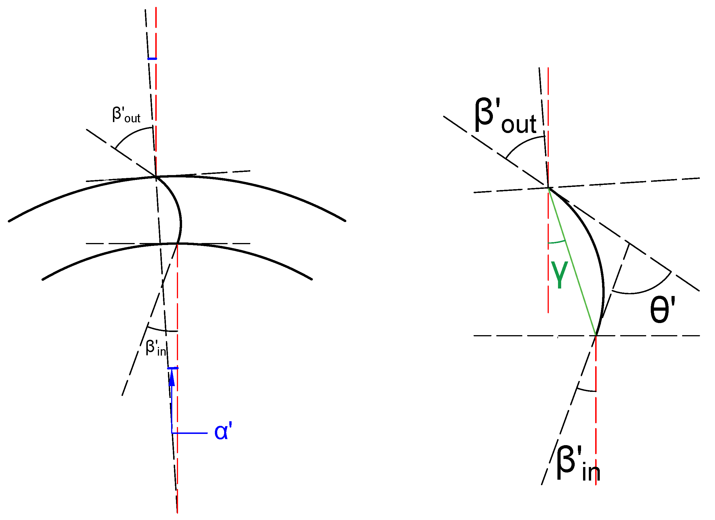
Besides the casing geometry, one should highlight that the aerodynamic profile of the blades is the basis of the cascade principles. Many parameters should be determined such as the stagger angle () and the camber angle (). Figure 5 depicts each parameter.
2.2. Loss Models
Loss models are known for being a good alternative when it comes to evaluate machines’ performance. Many correlations are established for different turbomachines. The reason why it is possible to apply the loss models (already existing in the literature) to evaluate the CFF performance is based on the fact that CFFs are capable of sharing similarities with other mechanisms. However, an additional study is required to be able to fit the models to the CFF functioning principles.
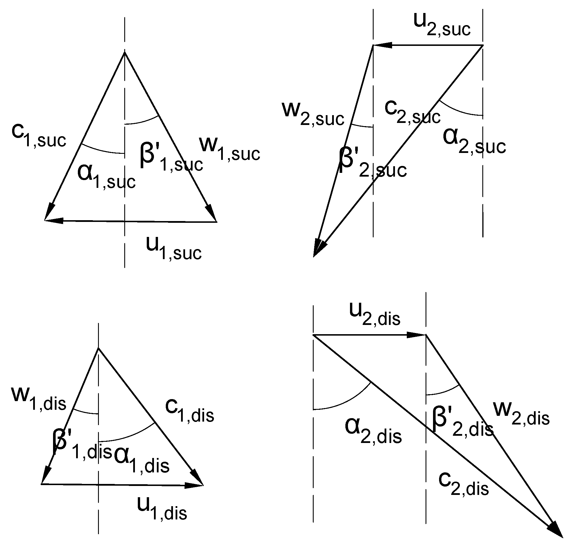
Even though some tiny vortices are formed in the edges of the suction and discharge arcs, the flow is considered equally distributed, and the velocity triangles should be determined according to each model. As summarized in Equations (1)–(3), both models share similarities in the computation of the Euler head, the total and static pressures, and the pressure and flow coefficients; nevertheless, the losses and the velocities are specific to each model:
The flow and pressure coefficients are defined as follows:
- ;
- ;
- ;
- ;
- .
As a note, is an unknown parameter that should be thoroughly analyzed.
2.2.1. Streamline Analysis
The loss model using the streamline analysis was firstly proposed by Kim et al. [21]. In fact, the fluid faces many obstacles when circulating trough the apparatus, and the pressure is lost in different forms. The first step should be the determination of the velocity triangles at the two boundaries of each stage (Figure 6). In this model, the air is supposed to flow tangentially to the blades with no deflection at the suction and discharge, meaning that the relative flow angle is equal to the blade angle. The flow angles are considered with their absolute value, and thus, no algebraic angle values are used. The loss models were extracted from the work of Oh et al. [23], where the authors indicated precisely the losses that result in the centrifugal compressor. Consequently, Oh and Chung [24] defined the losses in a centrifugal pump, as well as the formulas were slightly adjusted to fit the CFF design. A brief description, as well as the characteristics of the most important loss models are summarized in Table 1.
It is useful to note that following descriptions also exist for the models:
- Skin friction loss—first law: ;
- Skin friction loss—second law: ;
- Re-circulation loss: .
2.2.2. Cascade Principles Applied to Cross-Flow Fans
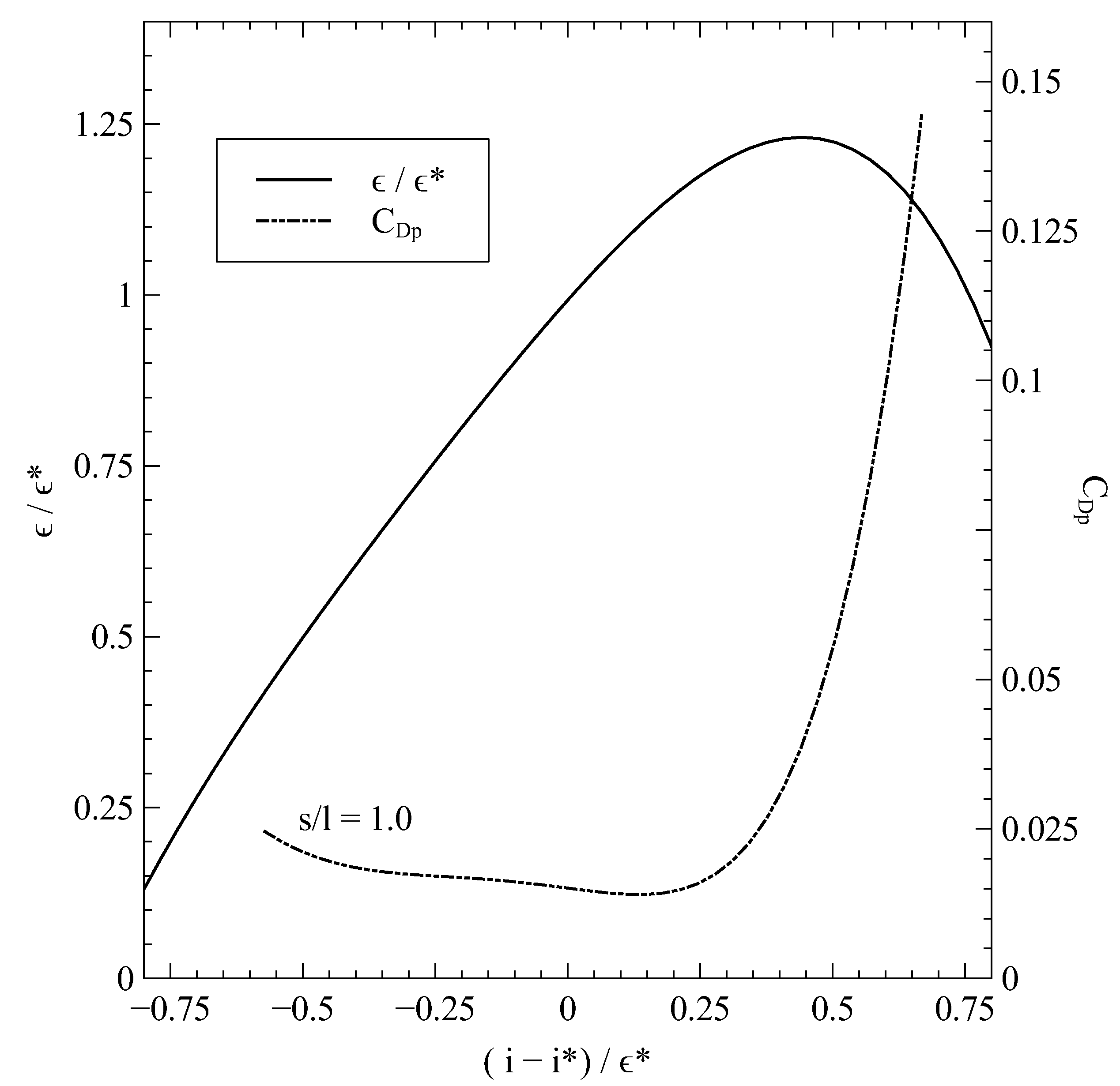
It is undeniable that the cascade principles marked a significant step in the turbomachines’ history. In fact, the study of cascades is based on the deviation of the flow direction from the blade wall. The gap between the fluid and the blade plays a key role to determine the ideal total pressure, the drag coefficient, and thus, the pressure loss. Hence, the total performance of the stage can be deduced. As a pioneer in this field, Howell developed a mathematical correlation to describe the pressure rise/loss in each stage of a turbomachine. Furthermore, efforts have been made to gather the characteristics of different types of turbomachines into one single curve (see Figure 7), which has been widely used by the industrial community over decades for the definition of blade geometry purposes. Using the cascade principles, the performance of an axial compressor has also been investigated. Howell attested that the global performance is governed by the characteristics of the nominal operating conditions, which are fixed at 80 percent of stalling [25,26]. In the same way, Dang and Bushnell [5] applied those principles to evaluate the performance of a cross-flow fan that was applicable in aircraft propulsion.
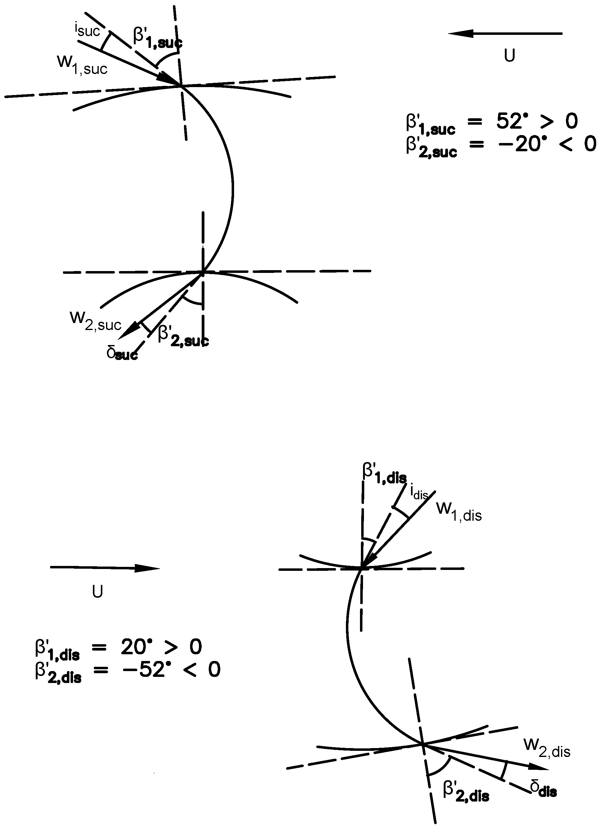
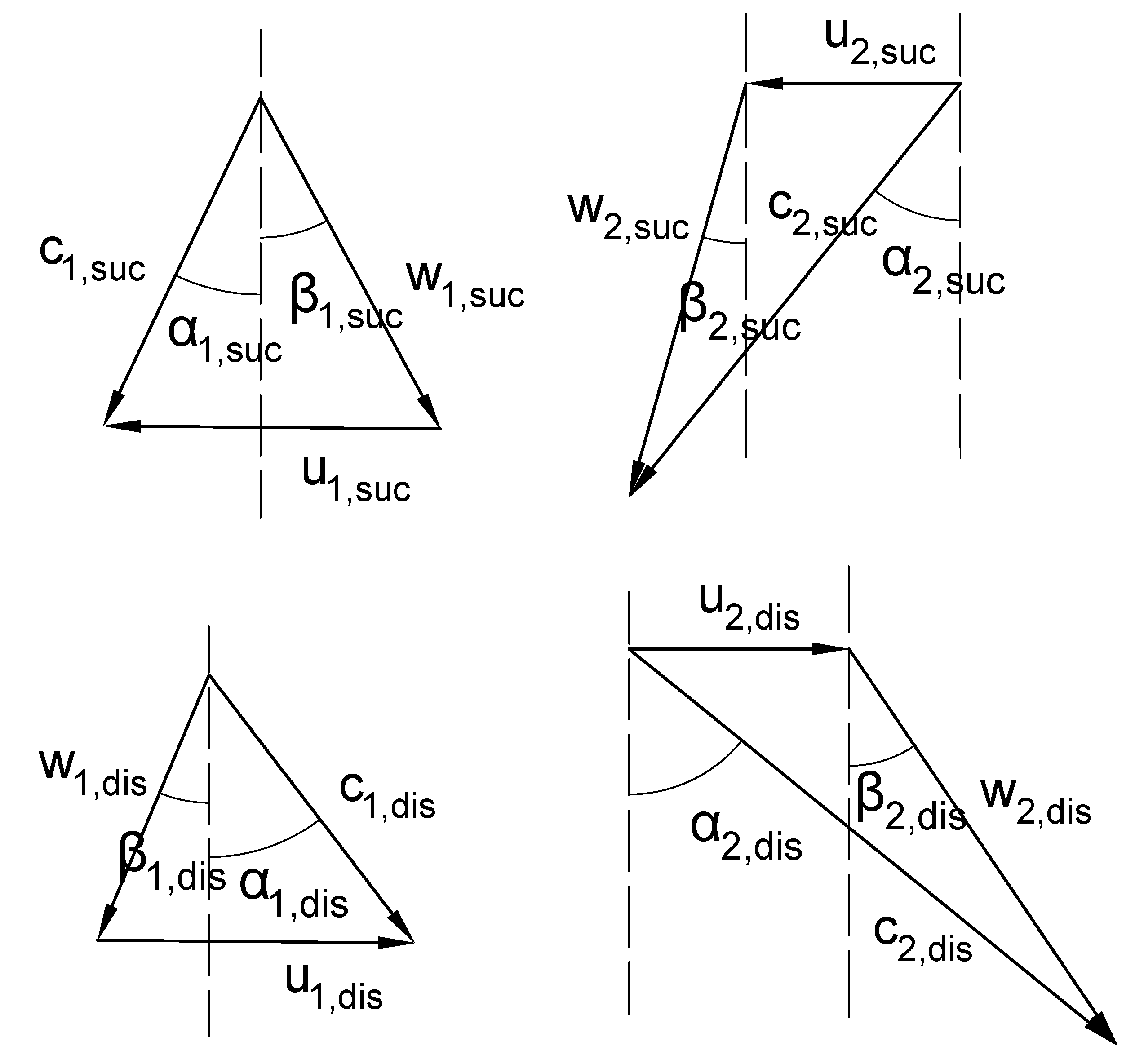
Howell referred to the difference between the air and blade angles at the inlet as the incidence angle: . He called the difference between the air and blade angles at the outlet “the deviation” . In addition to the deflection, this has been defined as the difference between the inlet and the outlet flow angles: . The relative flow angle was considered positive when it was measured against the direction of rotation (U). Meanwhile, the absolute flow angle has a positive sign when it is assessed in accordance with the direction of rotation (see Figure 8 and Figure 9).
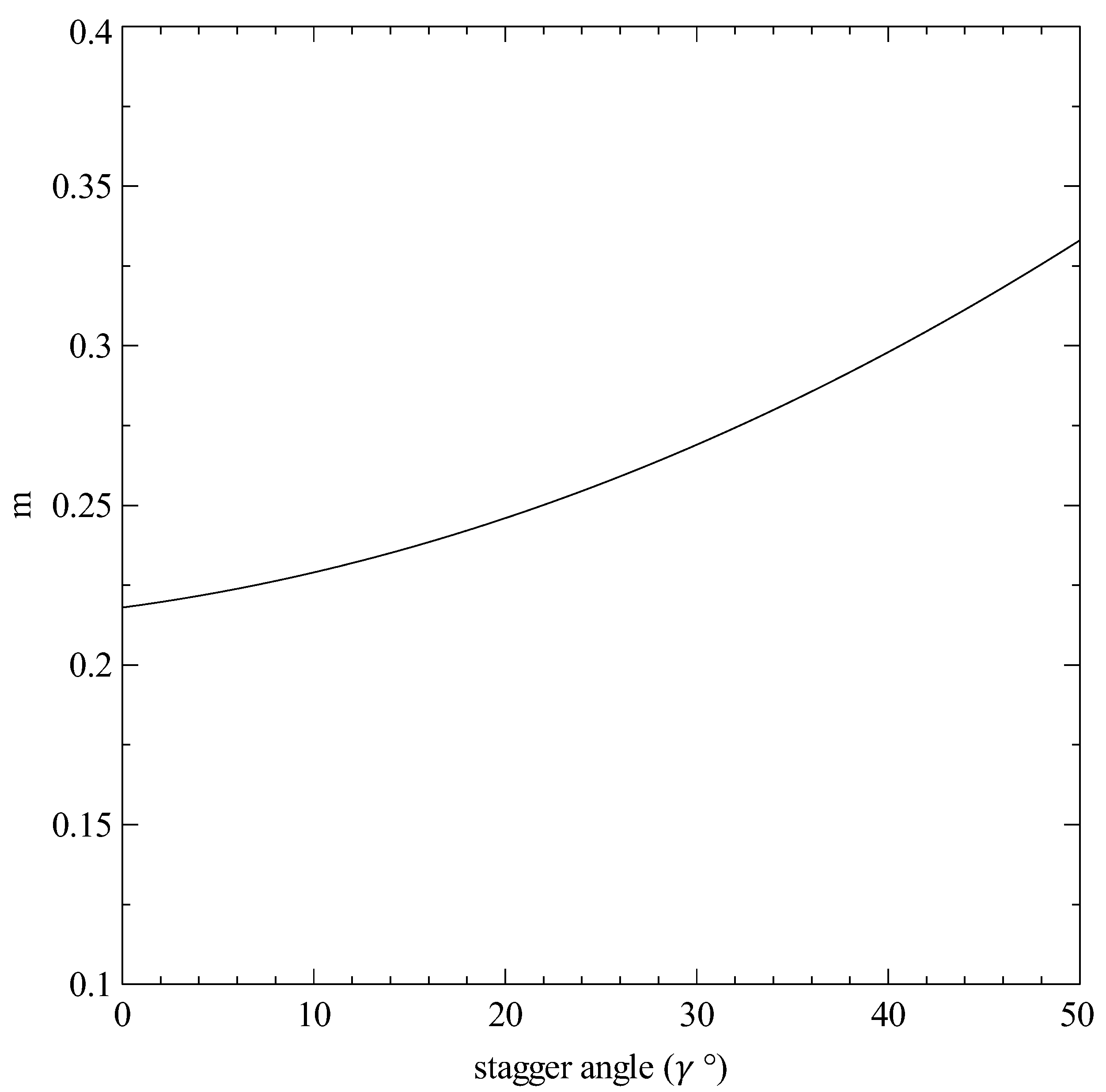
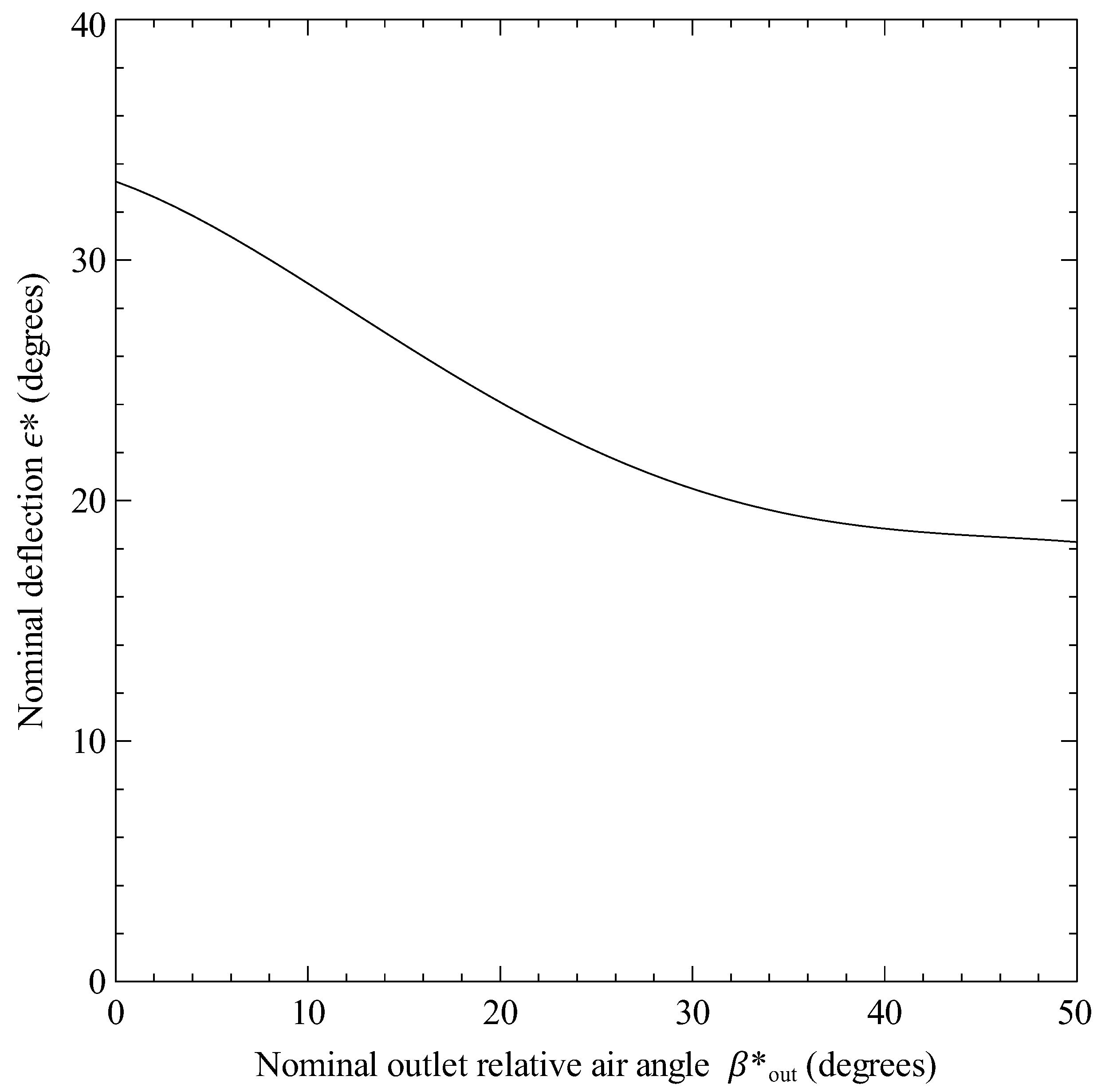
One should outline here that the nominal parameters are only dependent on the design of the blade; the nominal deviation is an explicit expression in terms of the camber and space-to-chord ratio:
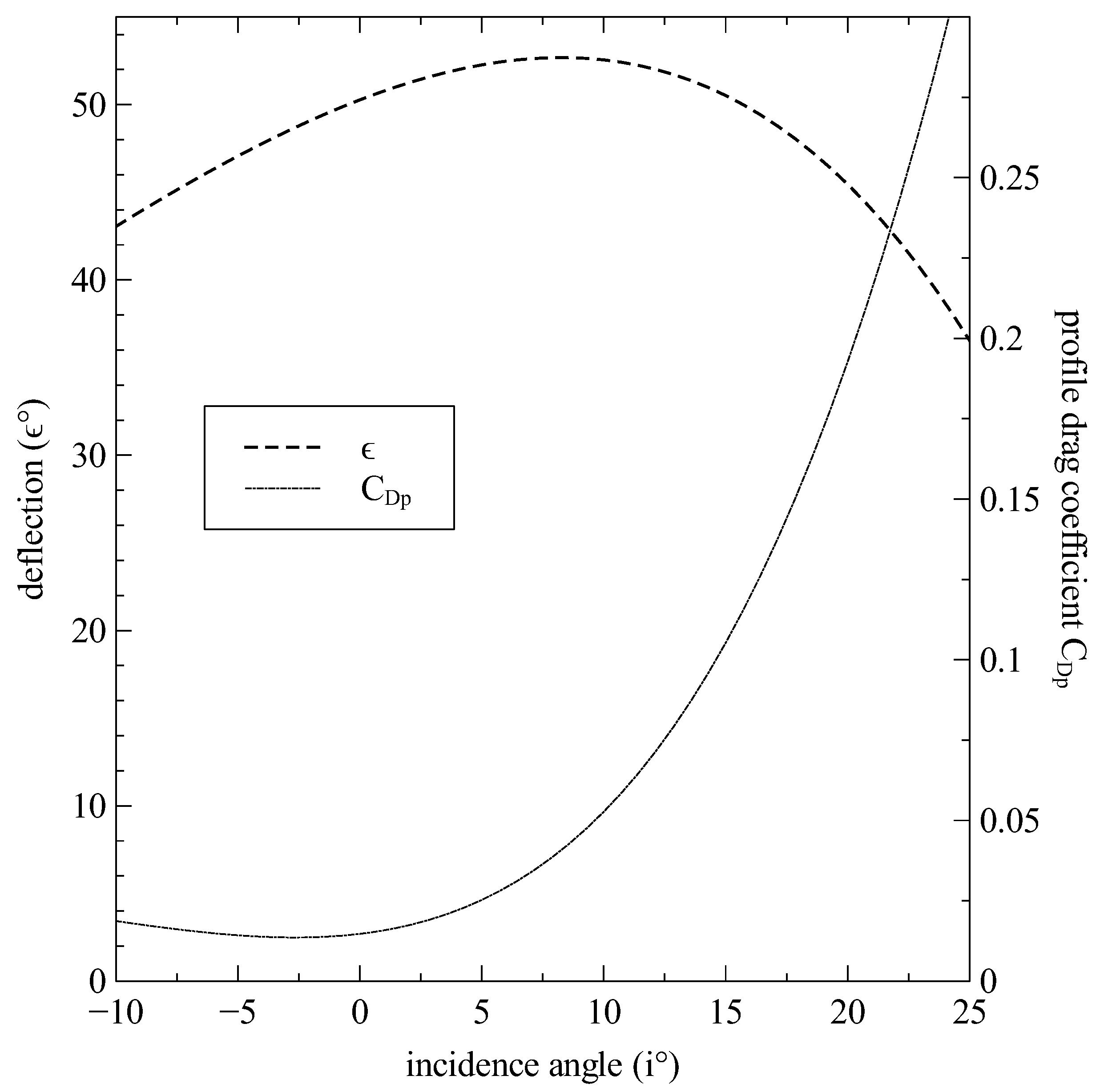
The value of the coefficient (m) and its variation as a function of the stagger angle () are shown in Figure 10 [27]. In Figure 11, the nominal deflection and its evolution against the nominal outlet flow angle are shown. Once the nominal deviation () is computed, the nominal outlet angle () can be calculated; the nominal incidence is then deduced (). Eventually, the required data in the nominal conditions are known, and the off-design cascade curve of each stage is ready to be plotted. Nevertheless, one should accept that using a specific curve for each stage fails to predict the performance with high precision. Obviously, the second stage critically influences the flow throughout the CFF; therefore, the off-design curve of the second stage (Figure 12) is used for both stages, providing a satisfactory level of accuracy.
Frequently, performance characteristics are appraised by assigning a value to the flow rate; however, by using the cascade principles, the flow rate is deduced by assigning a value to the incidence angle i of the first stage. Therefore, Howell fixed the degree of reaction for the stage at 50 percent and determined the radial velocity (in the case of an axial compressor: and ) as follows:
with:
- ;
- .
Owing to the inequality of U and throughout the blade channel in the CFF, this equation challenges the pertinence of its flow rate, or at least causes inappropriate results of the performance. Therefore, we administered a suitable approximation to calculate the radial velocity in the CFF, based on the following equations:
We obtain
Then, we suggest that
All of these assumptions are concluded as:
Seemingly, the new expression of revealed a great accuracy of the air flow within the machine, which seems to have good agreement with the global performance.
Following the assumptions and findings so far, it should be mentioned that the angular momentum is kept constant during the rotation; this leads us to assume that . This relation represents the link between the two stages and, thus, the flow angle (), as well as all the remaining angles deduced as follows:
where:
- ;
- (Figure 12);
- .
The drag coefficient () is a combination of several terms, as highlighted below:
- is the drag coefficient related to the blade profile, represented in the off-design curve, according to the incidence angle in each stage;
- corresponds to an additional loss related to the friction in the blade’s annulus, expressed as ;
- is the drag coefficient, which represents secondary losses, caused by small vortices that surround the blade wall, written as . defines the lift coefficient with the following equation:
- .
The pressure loss could directly be derived from the drag coefficient:
Given the above-mentioned explanations, as well as the included assumptions, almost all features have been taken into consideration. One can note that the ideal pressure rise (), the total pressure rise (), and the static pressure rise () can be determined for the prospective objectives.
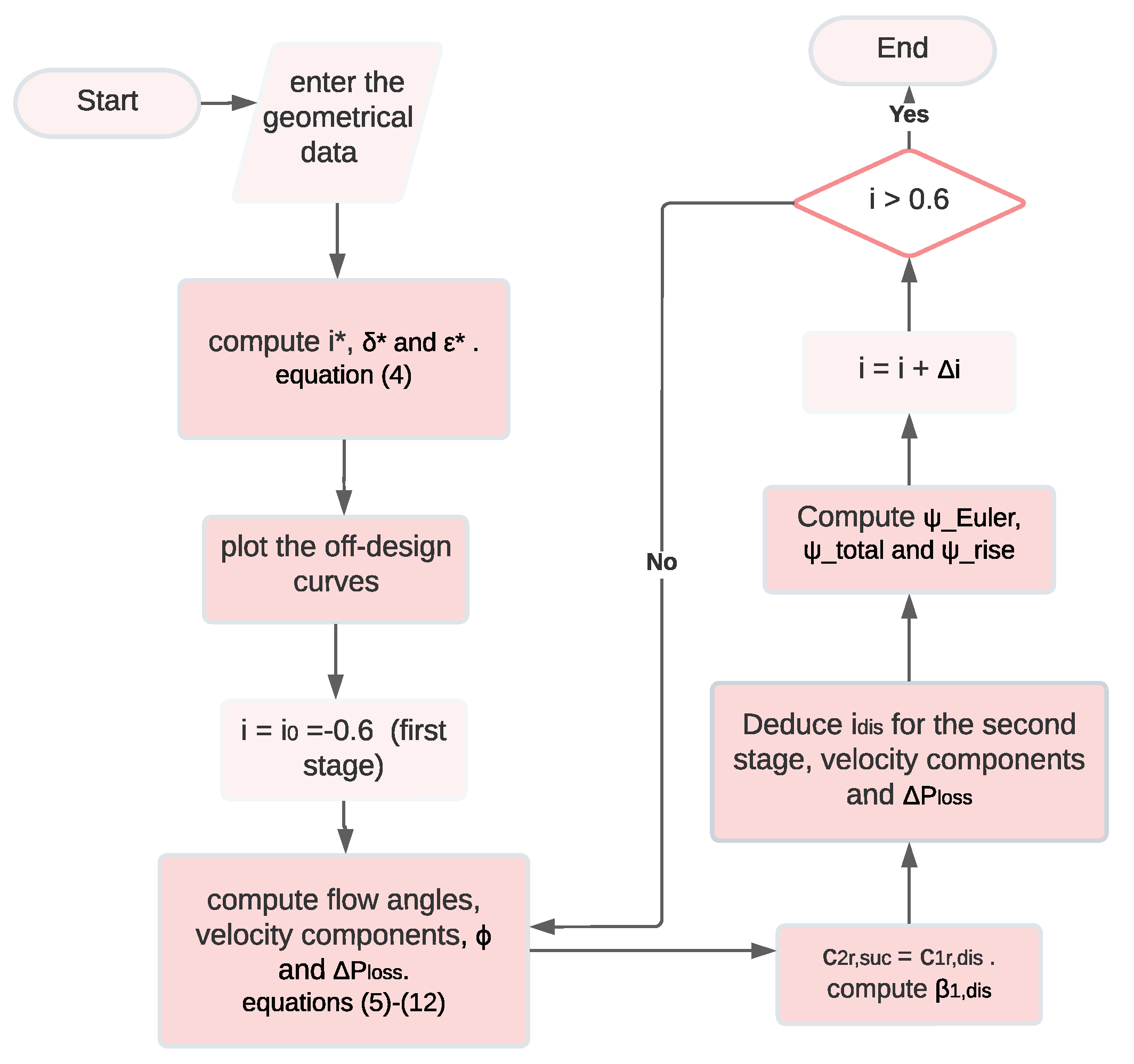
The cascade theory methodology used is presented in the following flowchart (Figure 13):
3. Results and Discussion
3.1. Performance–Pressure Curves’ Prediction
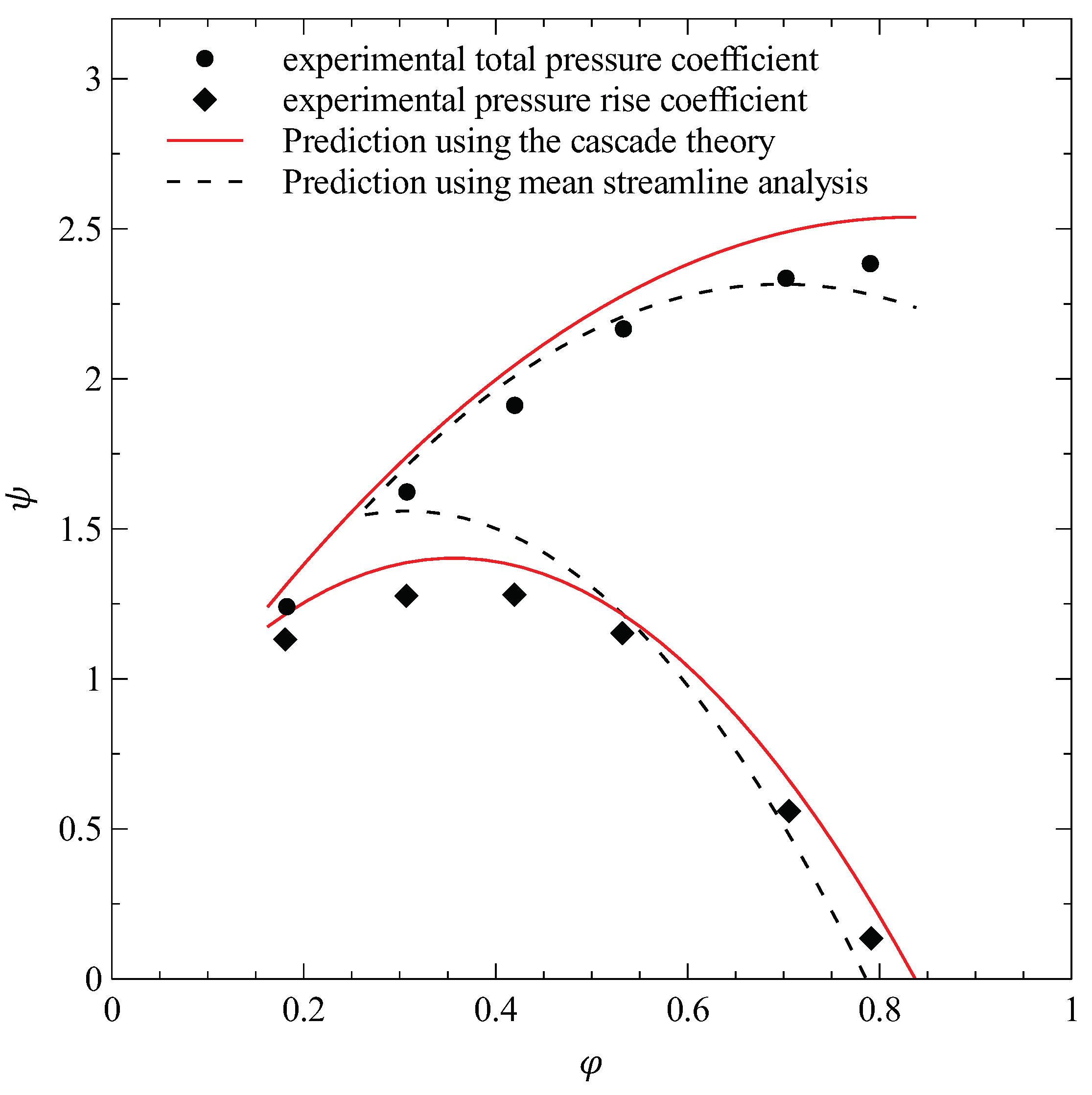
The loss models of the mean streamline and the cascade theory were applied in this study to predict the performance of the CFF. The two approaches were then compared to select the most convenient method that validates the experimental results. To perform an experimental validation, the obtained characteristics results of the performance were compared with the experimental results of Porter and Markland’s work [9] (see Figure 14).
The mean streamline analysis lies on the velocity triangles drawn in Figure 6. The loss correlations cited previously were used to compute the pressure loss. As illustrated in Figure 14, the main streamline analysis shows a good agreement with the experience in medium- and high-flow regions. However, at low flow rates, the curves invalidate the experience.
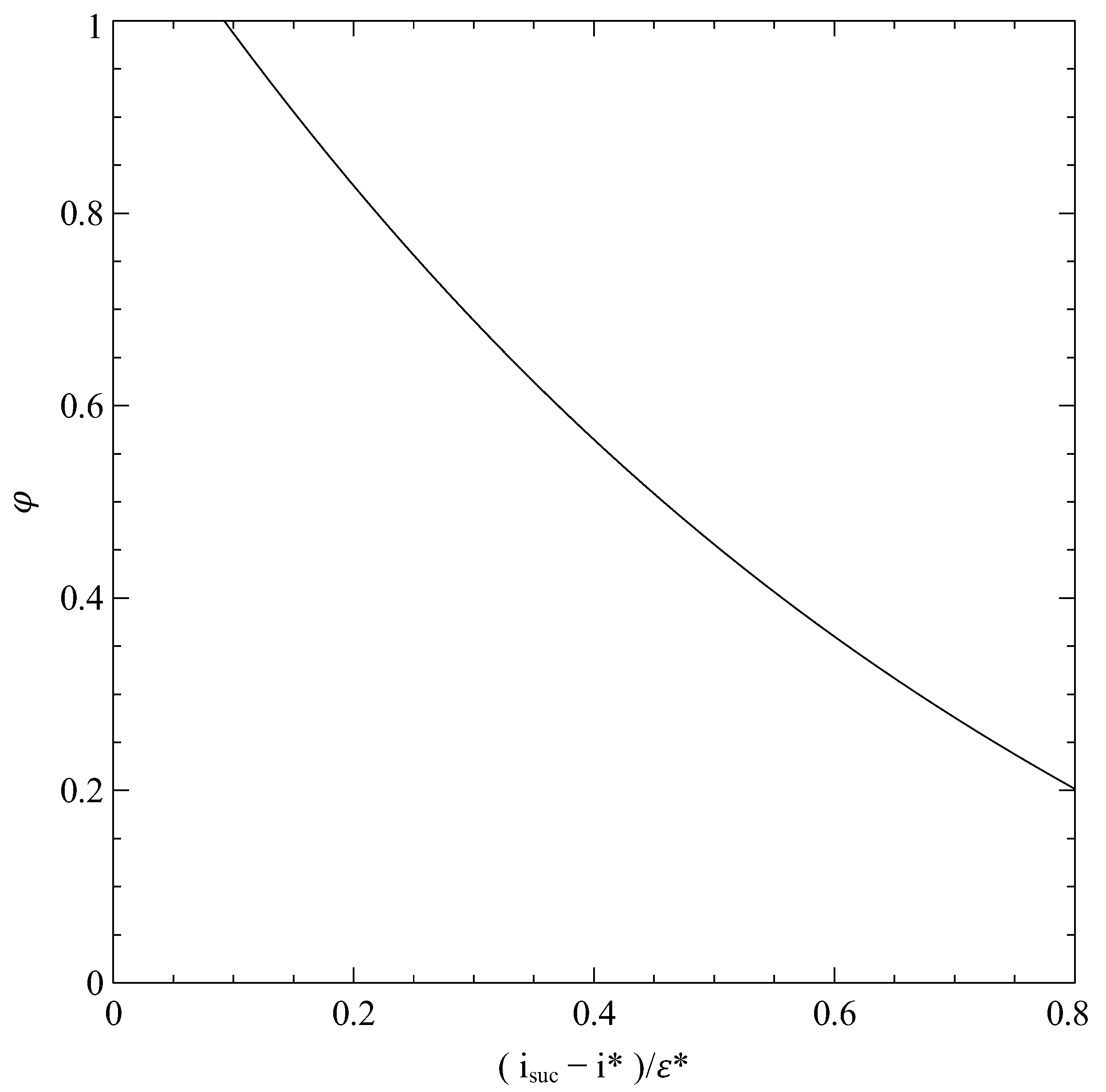
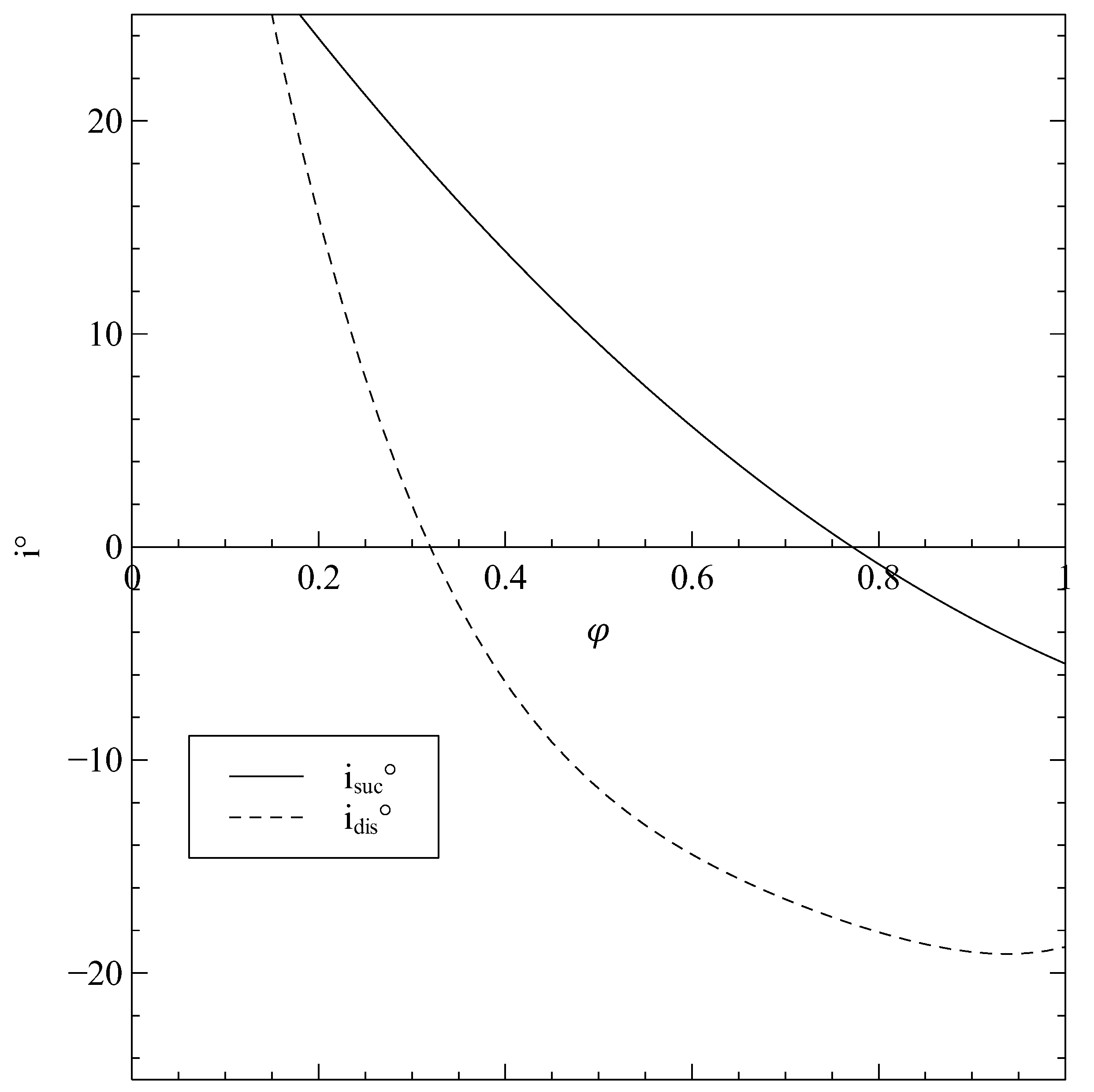
On the other hand, the prediction of performance using the cascade theory requires firstly deducing the curve of performance specific to the studied fan, as derived from Figure 7 and displayed in Figure 12. According to Howell, the normal operating domain for any machine is usually covered when the variable is situated between −0.6 and 0.6. In our case, the flow coefficient was computed based on this variable and revealed in Figure 15. In the same way, the incidence angles in the two stages are shown in Figure 16 as a function of the flow coefficient. The obtained results from the cascade theory match the experimental results in all the flow domain with an acceptable error. The cascade theory could be a suitable approach to predict the fan performance features of the CFF.
Furthermore, one should not forget that the efficiency is the most important characteristic that determines whether the machine corresponds to our requirements or not. Experience showed that a part of the energy provided to the fan serves to run the rotating impeller, and thus, the remaining part is absorbed by a generated vortex within the rotor. Scientists proposed a methodology that relies on the vortex power: Dang and Bushnell [5] suggested in their paper a correlation that approximates the efficiency , as shown in Equation (13):
where is the essential power to rotate the impeller and is the power absorbed by the vortex, and they are defined as follows:
Moreover, owing to the fact that the casing geometry varies from one fan to another and its shape highly affects the fan performance, a correcting coefficient was added to take into consideration the specific casing geometry. Dang and Bushnell [5] demonstrated that the vortex core can be considered as an ellipse with a fixed size, and they fixed then the equal to 0.7. These assumptions led the authors to satisfactory results that matched the experimental findings. In our case, we considered that the vortex has a fixed elliptical shape, and , as well as are its minor and major radii, respectively. When applying these parameters in the Eck/Laing fan, it must be pointed out that the generated results refuted the experimental findings at low and medium flow rates, as shown in Figure 17. However, as a disadvantage of this method, we should explore the CFF efficiency with more precision and develop a general method to obtain the fan efficiency curve.
3.2. Efficiency Investigation
The main aim of this part of our study is to develop an explicit expression that describes the efficiency of the Eck/Laing CFF. The latter has a different geometry than the one studied in the paper of Dang and Bushnell [5], which is why we should determine the specific to our case. The experimental data used in this section are the efficiency values collected by Porter and Markland [9], and our purpose is to find the corresponding to be able to satisfy this equality: . To do this and prior to proceeding with the resolution, some simplifications should be made.
By considering , we obtain:
The issue of finding the coefficients and for each flow rate is reduced to solving an optimization problem, where the objective function to minimize is the absolute error between the experimental and theoretical efficiencies: , with and , these two domains permit the vortex to cover up the whole impeller cross-section surface.
Due to its simplicity and efficiency, Particle Swarm Optimization (PSO) is suitable for this kind of optimization problem. PSO is a metaheuristic non-intrusive algorithm that is widely used in engineering, including the turbomachinery domain [28,29,30,31]. In 1995, Eberhart and Kennedy [32] attempted to develop an algorithm that describes the swarm motion of animals, such as bees, birds, or even fishes. Subsequently, this social behavior algorithm turned out to be a relevant tool in optimization. Its idea is to set a population of moving particles. In each iteration “t”, the position of each one is evaluated, and the particles will move toward the individual that has the closest position to the solution. The iterations will stop when the criteria are reached. The particle velocity during the displacement could be expressed as follows:
where , is the coefficient of inertia, which can be set to 0.5, and are the cognitive learning rate and the social learning rate, usually set equal to 2, and is a random number of a uniform distribution chosen between 0 and 1.
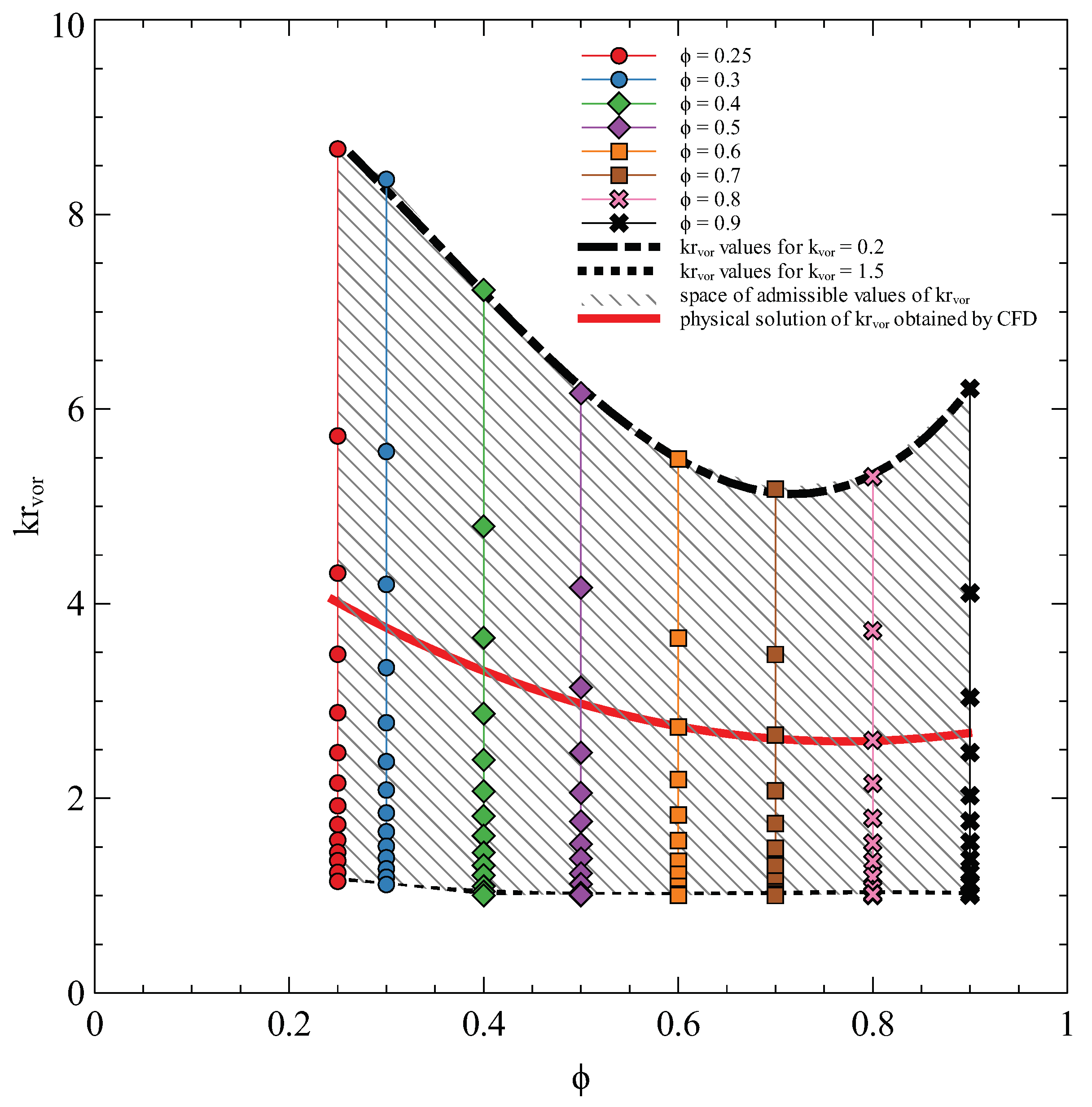
The resolution of the optimization problem using the experimental results gave us a space of admissible solutions of different couples of , as depicted in Figure 18. Owing to the poor interpretation that can be made by this space of solutions, we put in place a CFD method to refine them.
Numerical Simulation
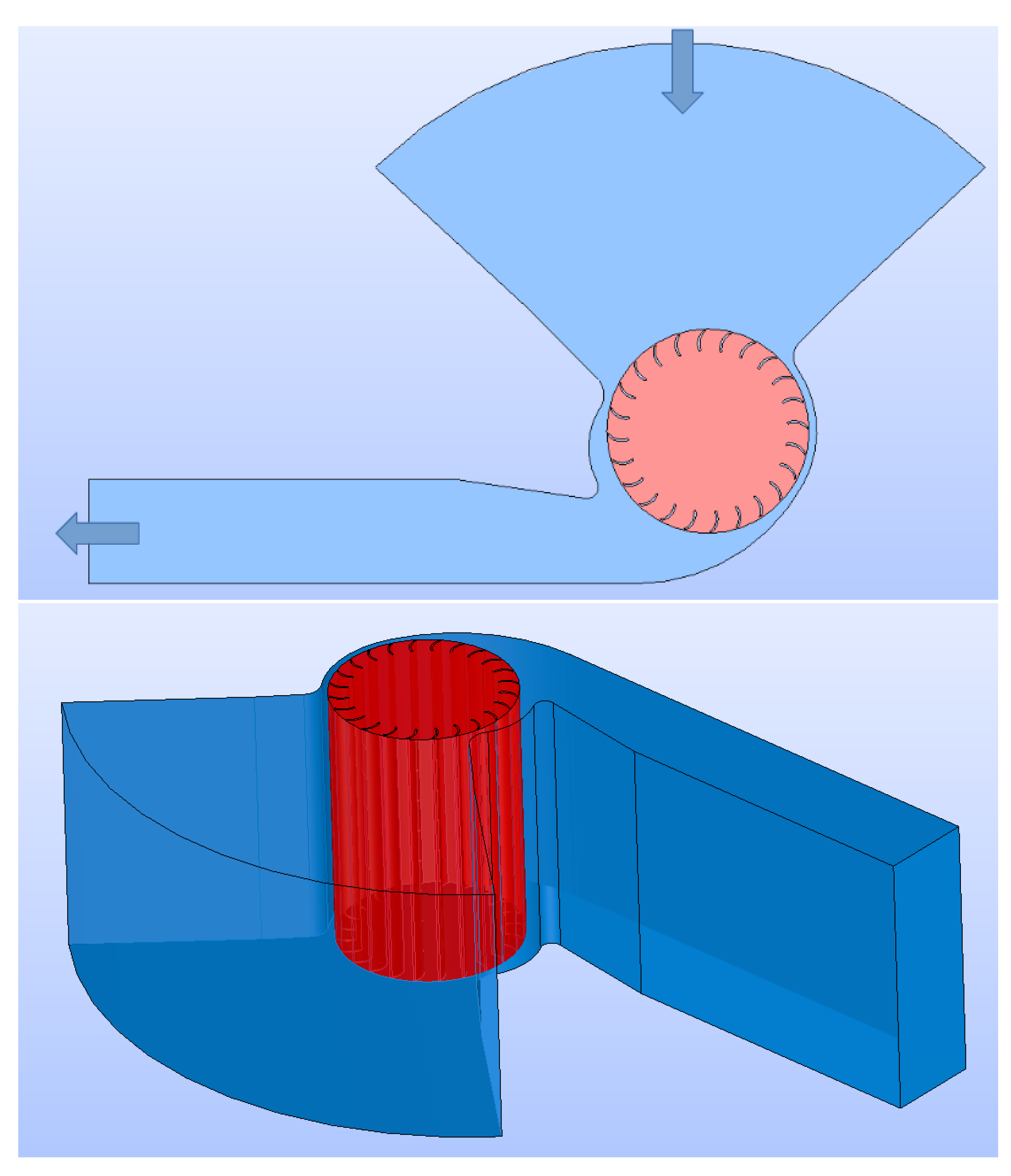
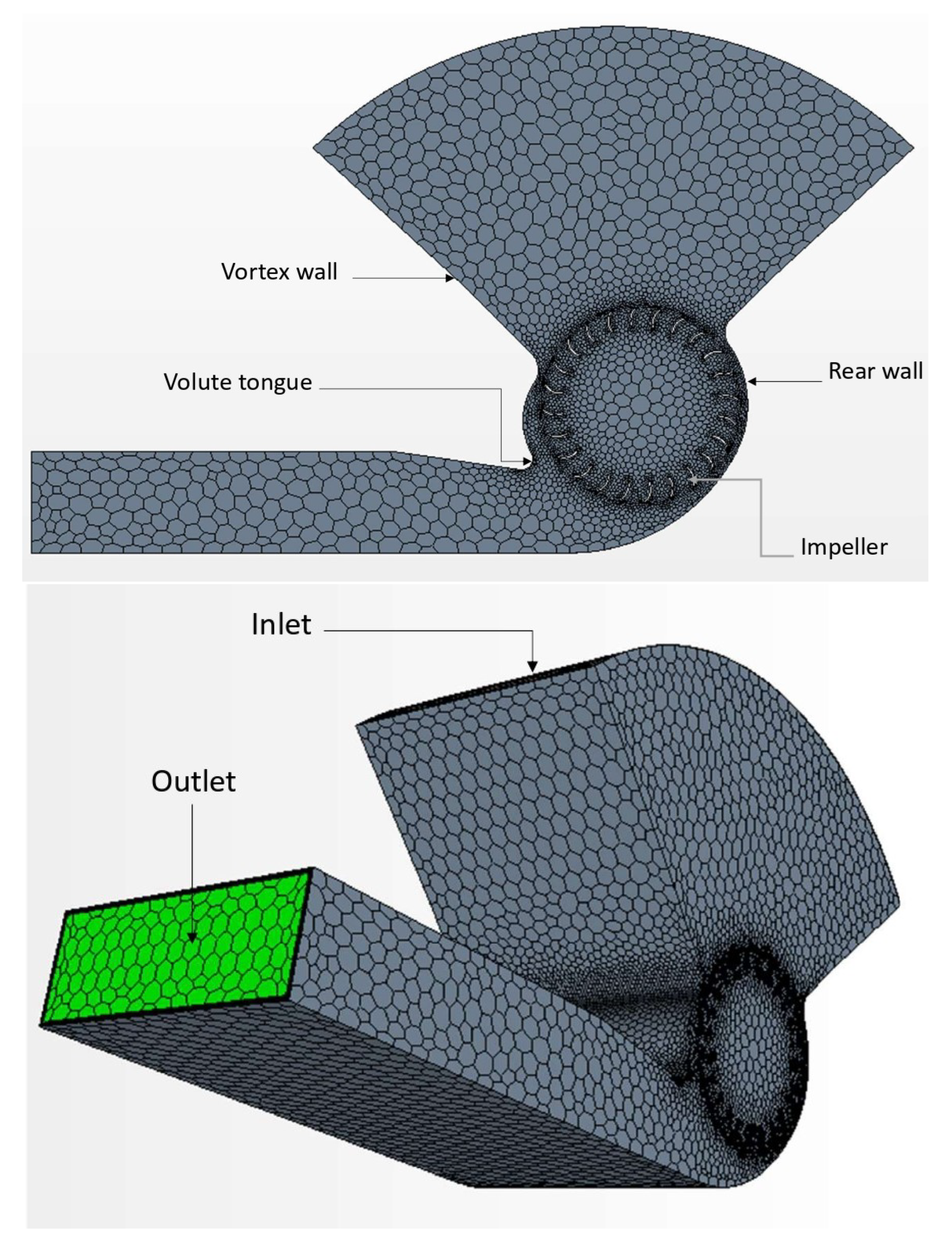
In order to find a unique couple of parameters for each flow rate, a CFD of the CFF was performed using Starccm+. The numerical model of the CFF is identical to the experimental one. The upstream and downstream boundaries of the fan were extended in order to avoid stiff boundary effects; see Figure 19. Mass flow and outlet boundary conditions were applied to the fan inlet and outlet, respectively.
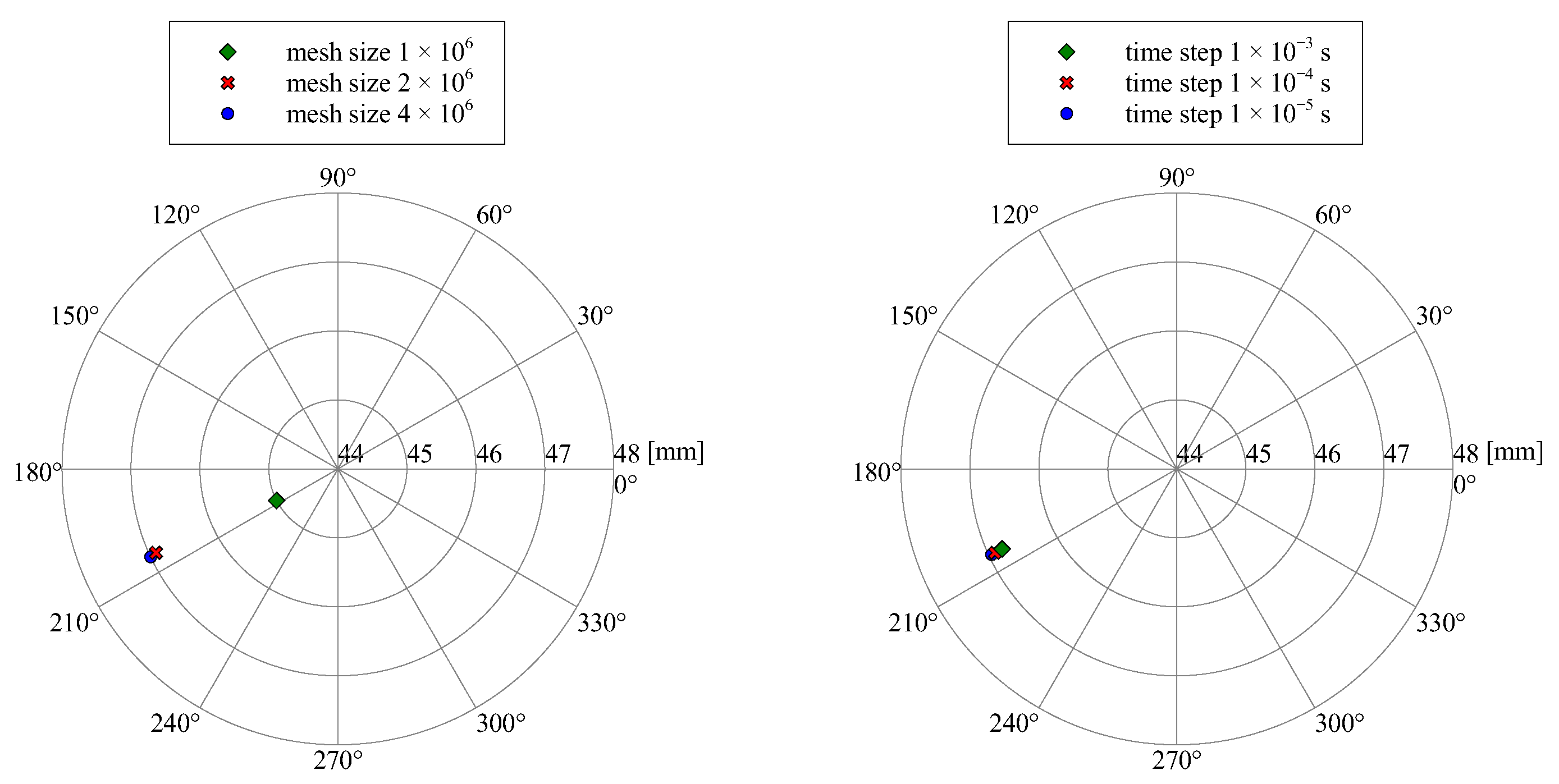
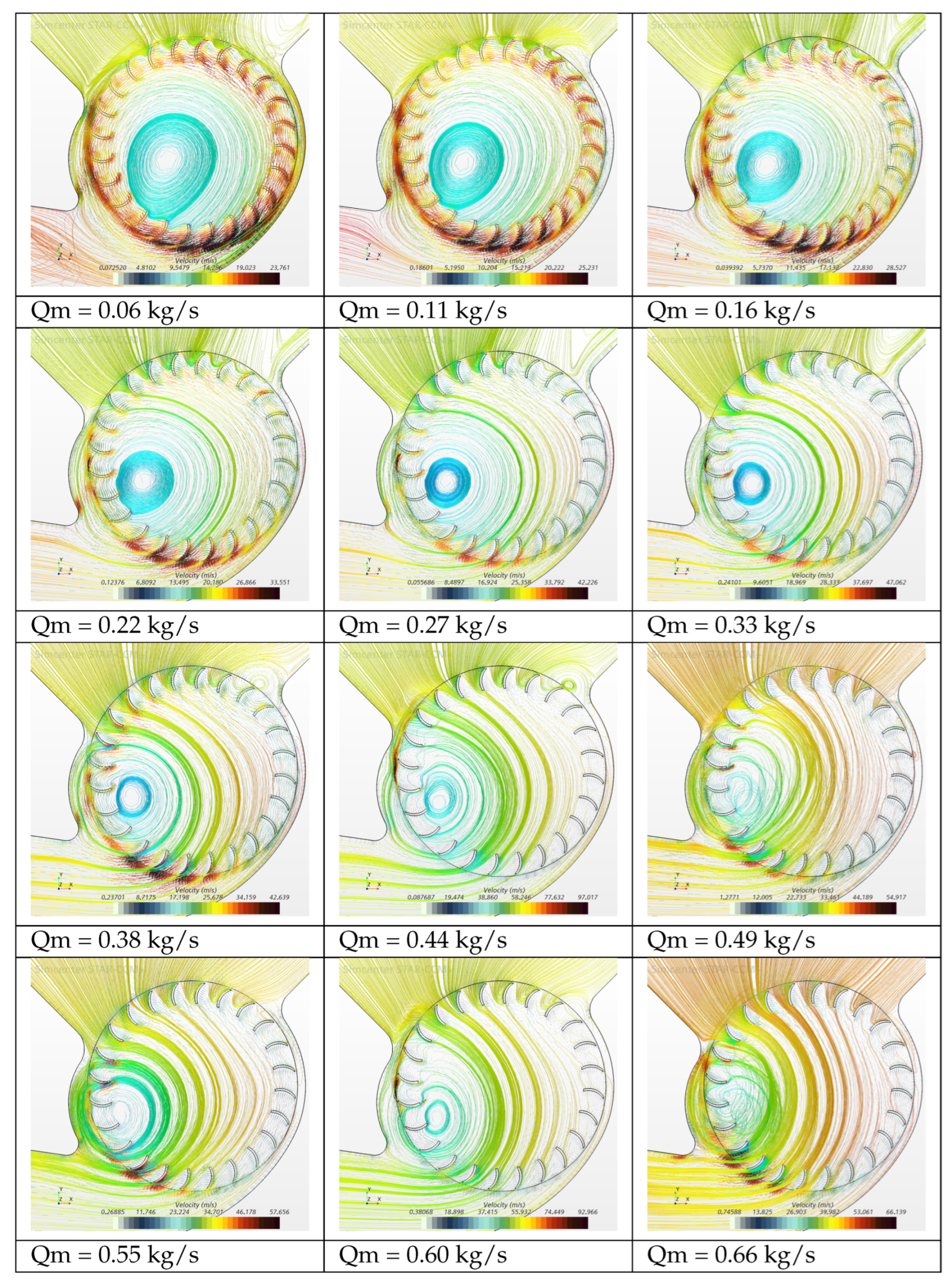
Preliminary results using a steady moving reference frame calculation were not conclusive because they are not physical; the calculation presented difficulties converging towards a stable and unique solution. In order to overcome this inconvenience, an unsteady calculation using a sliding mesh was carried out despite the fact that it was time and resource consuming. The SST turbulence model was used. A preliminary mesh size sensitivity analysis was carried out; see Figure 20—left. It showed that a grid of polyhedral cells (with five layers at the wall boundary layers) was a good compromise between calculation time and accuracy; see Figure 21. The parameter on the walls was varied from 0.3 to 70, with 90% of the meshes having a . A sensitivity analysis of time step is presented in Figure 20—right, and a time step of s was used to ensure 10 points per blade passage. The simulations were performed for 10 revolutions of the rotor. Finally, a segregated flow solver and second-order space order of accuracy were used, as well as an implicit time solver. The simulation was carried out for different mass flows starting from 0.06 to 0.66 kg/s, for both 1400 rpm and 2250 rpm rotor rotational velocities. The presented instantaneous streamlines were taken at the end of the last rotor revolution.
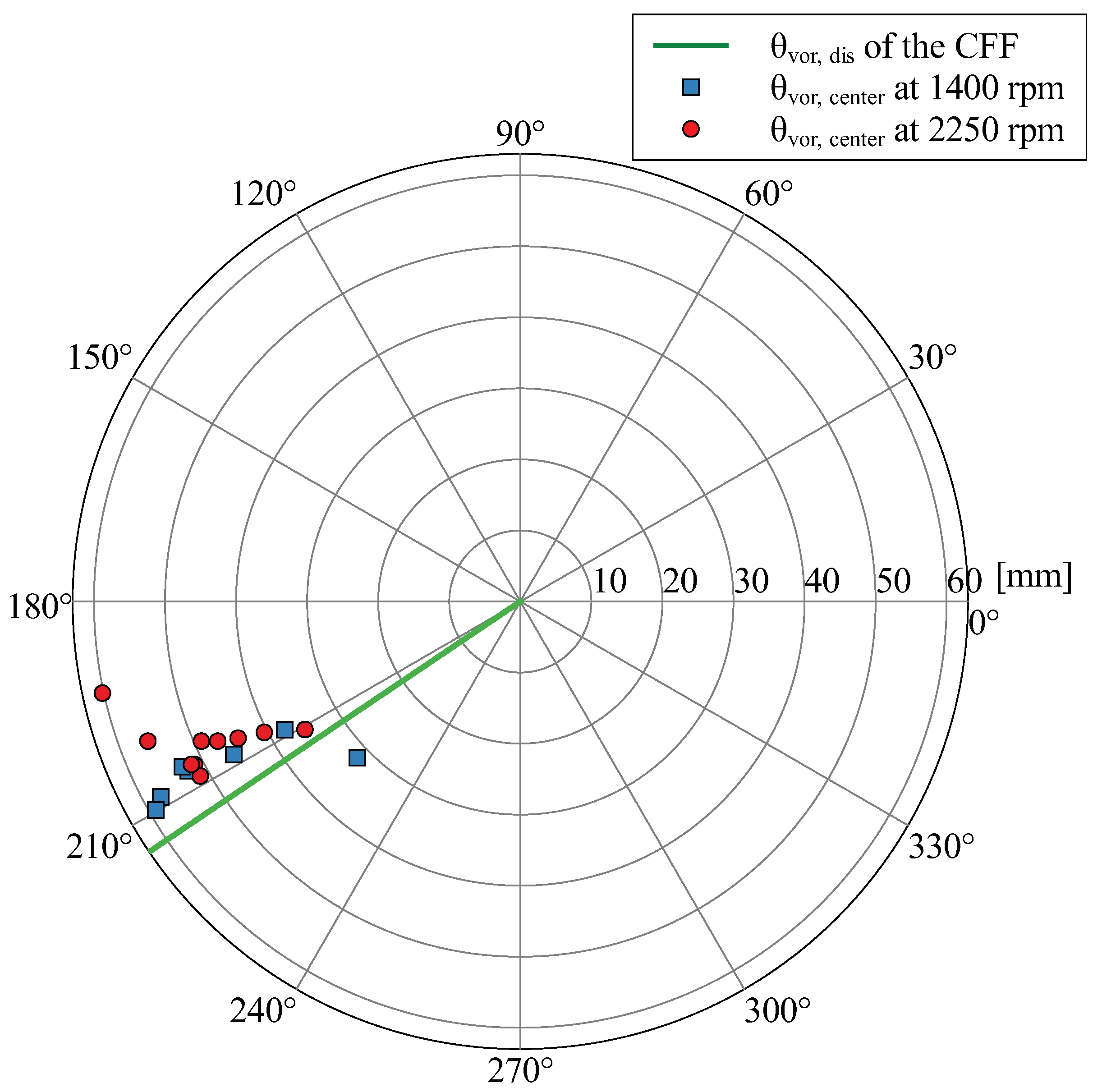
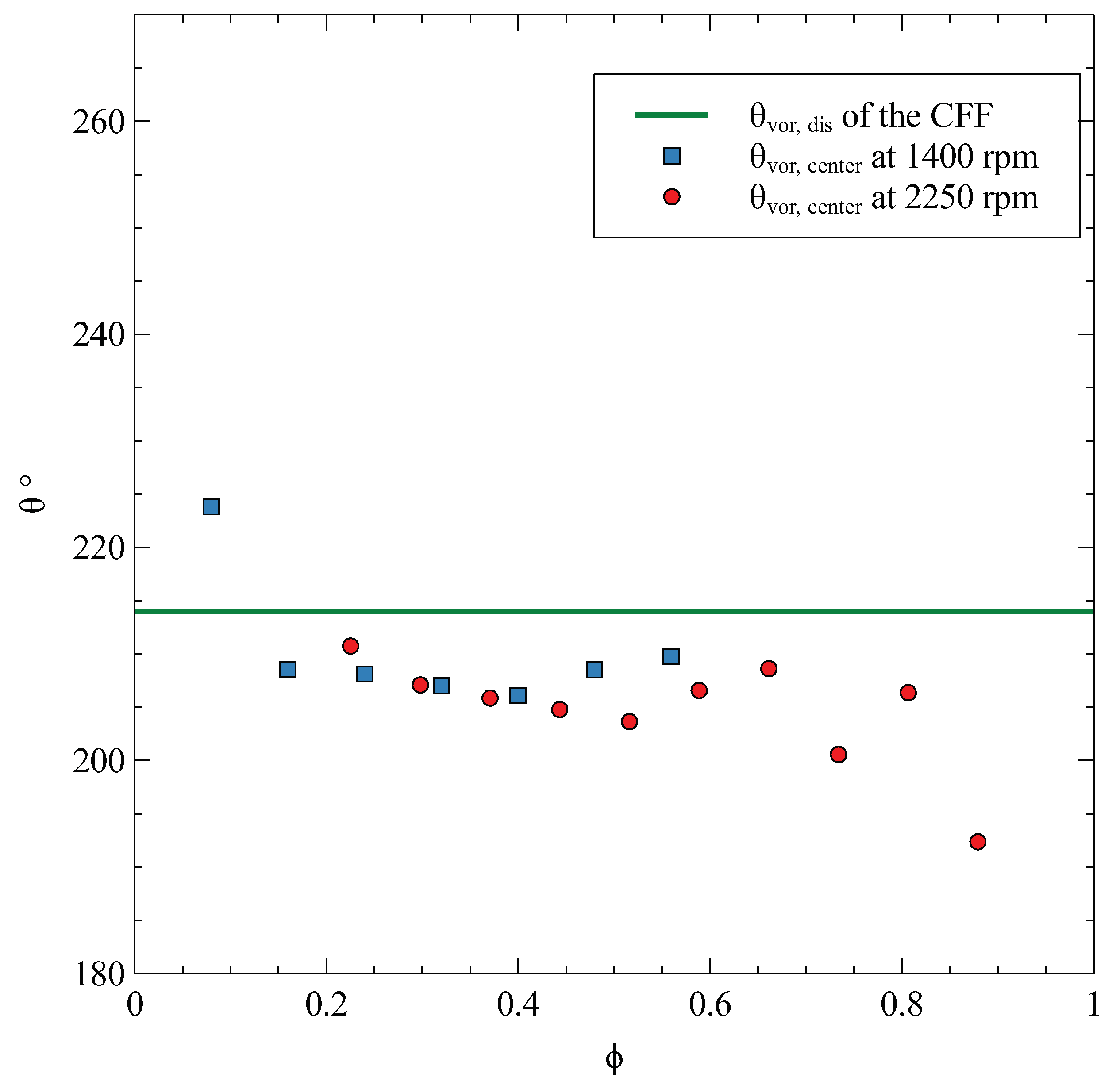
The data collected from the simulations were projected in a cross-section normal to the longitudinal axis, as shown in Figure 22. The streamlines delimit the re-circulation zone. We noticed that the vortex size became smaller whenever we increased the flow rate, and its center tended to move toward the rotor’s inner periphery. We can notice in Figure 23 and Figure 24 that the angular position of the vortex center is almost equal to (as defined in Figure 4) at low and medium flow rates. However, the center tends to move inside the vortex wall curvature at high flow rates.
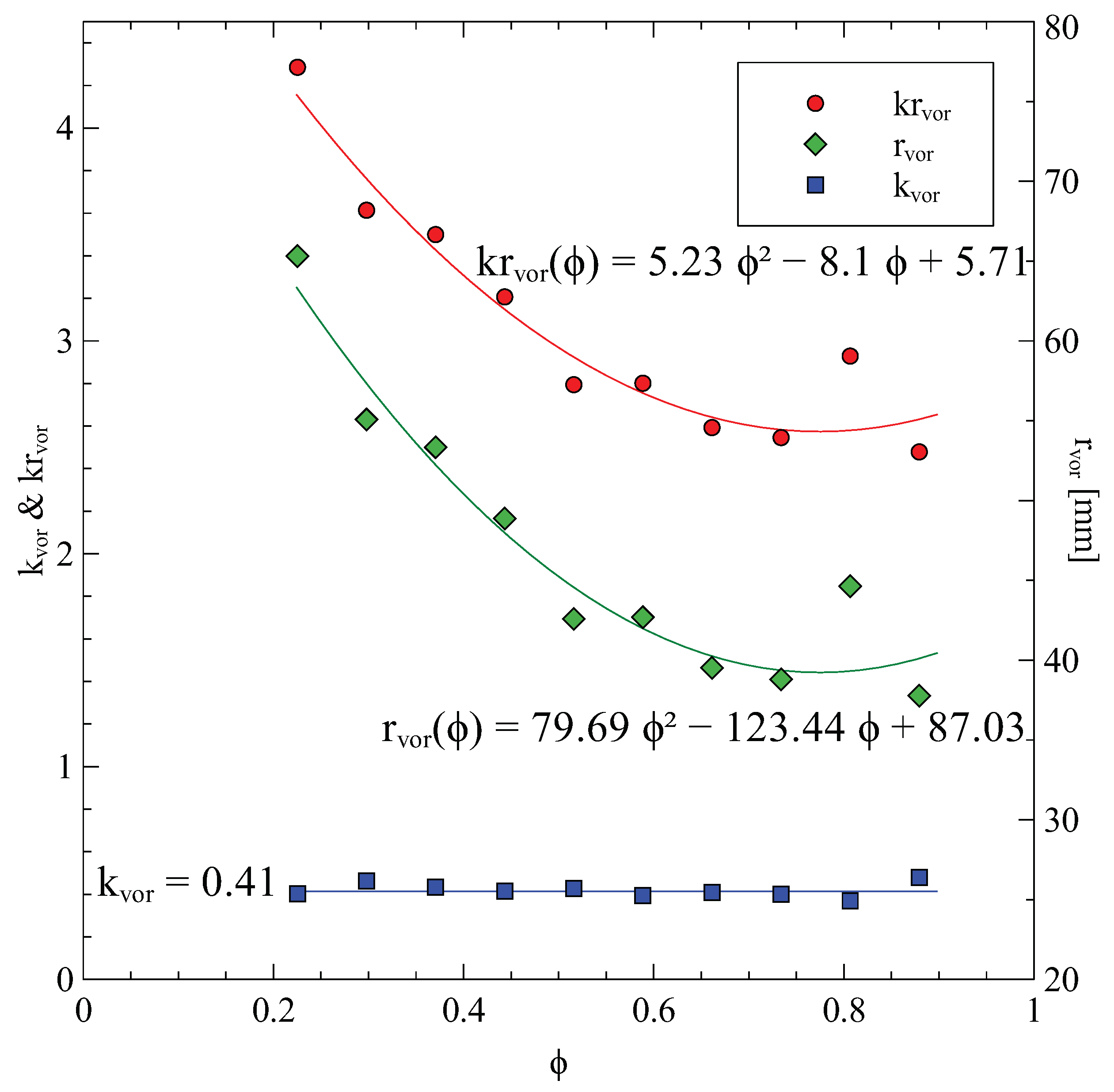
To investigate the efficiency, we measured the average vortex radius in each simulation and deduced the value of each time according to . The most satisfactory finding is that for each case, is around the same value, as indicated in Figure 25 and Figure 26, which means that specific to the Eck/Laing geometry is equal to 0.41.
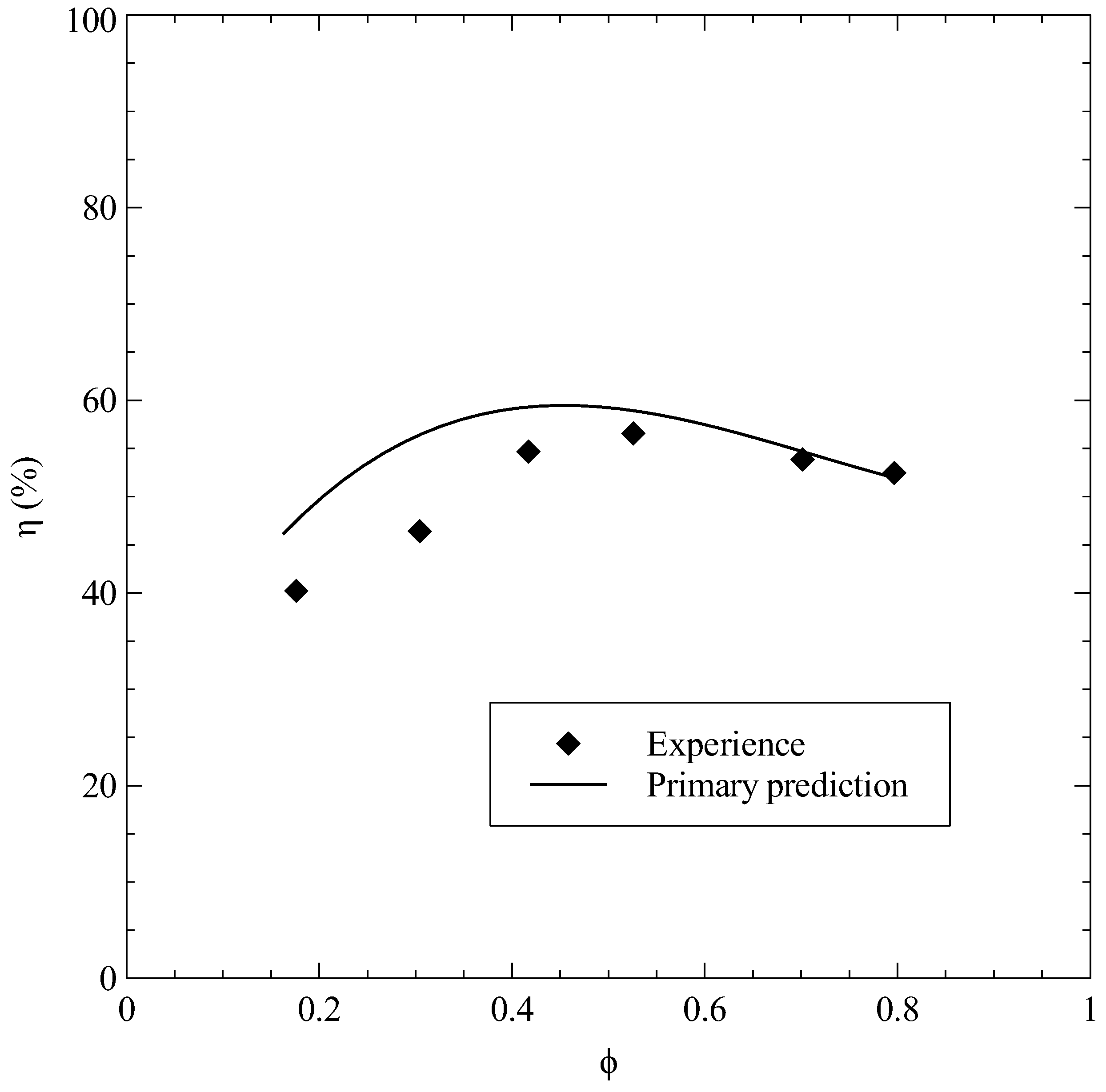
With reference to the above-mentioned results and by considering the great results obtained and shown in Figure 27, we concluded that the efficiency of the Eck/Laing fan can be expressed according to Equation (15), where and is defined with CFD analysis. The correlation is shown in Figure 25.
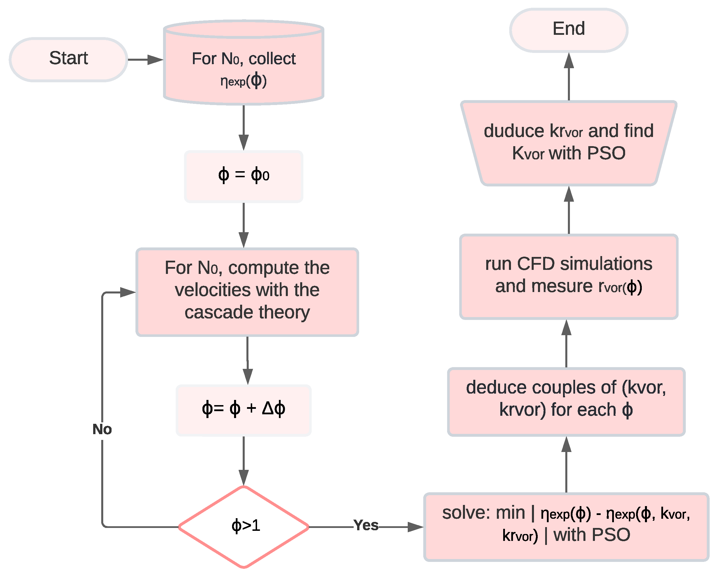
The efficiency correction procedure is presented in the following flowchart (Figure 28):
3.3. Discussion
The performance–pressure curves are of major importance for CFF manufacturers. The results showed that the loss model based on the mean streamline analysis is a good tool to predict them. However, it reveals a lack of precision in low and medium flow rates. On the other hand, the cascade principles showed a good agreement with the experimental results in all the flow domains, which makes the method more accurate to plot the performance–pressure curves for the Eck/Laing fan. Moreover, the efficiency is the most significant characteristic of the CFF, especially when the latter is involved in a cooling system. Its formulation is still a subject of study. Some works such as Dang and Bushnell [21] revealed that it is highly affected by the eccentric vortex power and size, and they established it by considering fixed flow regions inside the CFF. When we applied this theory to the Eck/Laing fan, it seemed that the plotted curve was not corresponding to the practical results. For this purpose, we decided to carry out further research to find the efficiency expression parameters using the experimental data. We put in place an optimization algorithm to determine the space of solutions of the expression parameters of the efficiency, then we explored the internal flow field with a CFD simulation to collect the vortex characteristics, to finally find the unique formulation of the efficiency of the Eck/Laing fan. This methodology is a combination of several studies with multiple aspects. We utilized semi-empirical theories in addition to an optimization procedure and numerical modeling. The outputs of this procedure are of extreme interest, and this approach can be an efficient strategy to predict the cross-flow fan performance.
4. Conclusions
This paper investigated the performance of CFFs using both analytical modeling and experimental data. A numerical methodology was described to predict the CFFs’ performance. To deduce the performance characteristics curves of CFFs, it appeared that the cascade theory validated well with the experimental results compared to that of the loss model. It is worth mentioning that the determination of the fan geometry is a prerequisite step.
Moreover, the literature provides a classical approximation of the CFF’s efficiency, which considers that the generated vortex within the rotor has a fixed center and size. Nonetheless, those characteristics vary and are still unknown so far, especially when the main vortex highly affects the CFF efficiency. The key contribution of this work is to model the efficiency by taking into account the variation of the vortex position and size. To do this, a multidisciplinary study was employed to obtain a general formulation of the efficiency of the Eck/Laing fan, the latter being the most used CFF in Europe. This work relies on experimental data, which were firstly used to obtain a space of solutions of the efficiency parameters using an optimization algorithm (PSO). This space was then refined with CFD simulations to obtain a unique couple of efficiency parameters. The results agreed with the experimental data with high accuracy, as shown in the above figures. To the best of our knowledge, this is the first study to describe precisely the cascade principles applied to cross-flow fans, and such techniques have not previously been employed to formulate the CFF’s efficiency by taking into account the dynamics of the vortex. As a result of those works, we proposed a robust methodology of performance analysis that permits speeding up the design cycle of cross-flow fans. The next step should be to explore the vortex attitude and power to be able to set a general methodology that describes the CFF performance for any available geometry on the market.
Author Contributions
Conceptualization, R.M.H. and S.K.; methodology, S.K. and R.M.H.; software, R.M.H., S.K. and M.A.A.C.; validation, S.K. and R.M.H.; formal analysis, R.M.H.; investigation, R.M.H., S.K. and H.R.V.; resources, S.K., R.M.H. and H.R.V.; writing—original draft preparation, R.M.H.; writing—review and editing, S.K. and H.R.V.; visualization, R.M.H., S.K. and M.A.A.C.; supervision, S.K., F.B. and I.B. All authors have read and agreed to the published version of the manuscript.
Funding
This research received no external funding.
Institutional Review Board Statement
Not applicable.
Informed Consent Statement
Not applicable.
Data Availability Statement
The experimental data used in this work come from the study of Porter and Markland [9], https://doi.org/10.1243/JMES_JOUR_1970_012_071_02; The graphs related to the cascade theory were extracted from the paper of Howell [25] https://doi.org/10.1243/PIME_PROC_1945_153_049_02.
Conflicts of Interest
The authors declare no conflict of interest.
Abbreviations
The following abbreviations are used in this manuscript:
| Symbols | |
| A | air |
| c | absolute velocity |
| friction coefficient | |
| g | gravity acceleration |
| h | height |
| i | incidence angle |
| k | coefficient |
| kr | radius coefficient |
| L | length |
| N | rotational speed (rpm) |
| S | arc/section |
| s/l | space-to-chord ratio |
| U, u | rotational speed |
| w | relative velocity |
| Z | blades number |
| absolute flow angle | |
| angle defined in Figure 5 | |
| relative flow angle | |
| blade angle | |
| stagger angle | |
| deviation | |
| pressure head | |
| pressure gradient | |
| deflection | |
| efficiency | |
| angle/angular coordinate | |
| camber angle | |
| power | |
| air density | |
| flow coefficient | |
| pressure coefficient | |
| Superscripts | |
| nominal operating conditions | |
| Subscripts | |
| 1 | inlet |
| 2 | outlet |
| bl | blade |
| center | vortex center |
| dif | diffuser |
| dis | second stage (discharge) |
| Euler | Euler head |
| exit | wind tunnel exit |
| id | ideal |
| in | rotor inner periphery |
| loss | pressure loss/head loss |
| m | average |
| mid | blade midpoint |
| out | rotor outer periphery |
| r | radial component |
| rc | re-circulation |
| rot | rotational |
| sf | skin friction |
| stat | static |
| suc | first stage (suction) |
| th | theoretical |
| thr | throat |
| tot | total |
| vol | volute |
| vor | vortex/vortex wall |
| tangential component |
Appendix A
This is a numerical example of the calculation of the total pressure and the pressure rise for a given incidence angle, using cascade principles applied in the Eck/Laing CFF. The first thing to begin with is the characteristic angles and the angles at the nominal condition. The camber angle for our blade profile is expressed as:
- ,
and the stagger angle is determined as follows:
In the following example, we consider the case where . It is noticeable that the numerical results shown in the table are rounded.

References
- Mortier, P. Fan or Blowing Apparatus. U.S. Patent US507445A, 24 October 1893. [Google Scholar]
- Shih, Y.C.; Hou, H.C.; Chiang, H. On similitude of the cross flow fan in a split-type air-conditioner. Appl. Therm. Eng. 2008, 28, 1853–1864. [Google Scholar] [CrossRef]
- Endoh, H.; Enami, S.; Izumi, Y.; Noguchi, J. Experimental Study on the Effects of Air Flow from Cross-Flow Fans on Thermal Comfort in Railway Vehicles. In Proceedings of the Congress of the International Ergonomics Association, Florence, Italy, 26–30 August 2018; Springer: Berlin/Heidelberg, Germany, 2018; pp. 379–388. [Google Scholar]
- Gossett, D.H. Investigation of Cross Flow Fan Propulsion for Lightweight VTOL Aircraft; Technical Report; Naval Postgraduate School: Monterey, CA, USA, 2000. [Google Scholar]
- Dang, T.Q.; Bushnell, P.R. Aerodynamics of cross-flow fans and their application to aircraft propulsion and flow control. Prog. Aerosp. Sci. 2009, 45, 1–29. [Google Scholar] [CrossRef]
- Mazumder, M.A.Q.; Golubev, V.; Gudmundsson, S. Parametric Study of Aerodynamic Performance of an Airfoil with Active Circulation Control using Leading Edge Embedded Cross-Flow Fan. In Proceedings of the AIAA Scitech 2019 Forum, San Diego, CA, USA, 7–11 January 2019. [Google Scholar] [CrossRef] [Green Version]
- Kummer, J.D.; Dang, T.Q. High-lift propulsive airfoil with integrated crossflow fan. J. Aircr. 2006, 43, 1059–1068. [Google Scholar] [CrossRef]
- Gologan, C.; Mores, S.; Steiner, H.; Seitz, A. Potential of the cross-flow fan for powered-lift regional aircraft applications. In Proceedings of the 9th AIAA Aviation Technology, Integration, and Operations Conference (ATIO) and Aircraft Noise and Emissions Reduction Symposium (ANERS), Hilton Head, SC, USA, 21–23 September 2009; p. 7098. [Google Scholar]
- Porter, A.; Markland, E. A study of the cross flow fan. J. Mech. Eng. Sci. 1970, 12, 421–431. [Google Scholar] [CrossRef]
- Preszler, L.; Lajos, T. Experiments for the development of the tangential flow fan. In Proceedings of the 4th Conference on Fluid Machinery, Budapest, Hungary, 11–16 September 1972; pp. 1071–1082. [Google Scholar]
- Murata, S.; Nishihara, K. An experimental study of cross flow fan: 1st report, effects of housing geometry on the fan performance. Bull. JSME 1976, 19, 314–321. [Google Scholar] [CrossRef]
- Tanaka, S.; Murata, S. Scale Effects in Cross Flow Fans: Effects of Fan Dimensions on Flow Details and the Universal Representation of Performances. JSME Int. J. Ser. B Fluids Therm. Eng. 1995, 38, 388–397. [Google Scholar] [CrossRef] [Green Version]
- Zhang, W.; Yuan, J.; Si, Q.; Fu, Y. Investigating the In-Flow Characteristics of Multi-Operation Conditions of Cross-Flow Fan in Air Conditioning Systems. Processes 2019, 7, 959. [Google Scholar] [CrossRef] [Green Version]
- Coester, R. Theoretische und Experimentelle Untersuchungen an Querstromgebläsen. Ph.D. Thesis, ETH Zurich, Zurich, Switzerland, 1959. [Google Scholar]
- Ikegami, H.; Murata, S. A Study of Cross Flow Fan (I. A Theoretical Analysis). Technol. Rep. Osaka Univ. 1966, 16, 556–578. [Google Scholar]
- Lazzarotto, L.; Lazzaretto, A.; Martegani, A.; Macor, A. On Cross-Flow Fan Similarity: Effects of Casing Shape. J. Fluids Eng.-Trans. ASME 2001, 123, 523–531. [Google Scholar] [CrossRef]
- Yamafuji, K. Studies on the flow of cross-flow impellers: 1st report, experimental study. Bull. JSME 1975, 18, 1018–1025. [Google Scholar] [CrossRef]
- Lajos, T. Investigation of the Flow Characteristics in the Impeller of the Tangential Fan. In Proceedings of the 5th Conference on Fluid Machinery, Budapest, Hungary, 15–20 September 1975; Volume 567. [Google Scholar]
- Tanaka, S.; Murata, S. Scale Effects in Cross-Flow Fans: Effects of Fan Dimensions on Performance Curves. JSME Int. J. Ser. B Fluids Therm. Eng. 1994, 37, 844–852. [Google Scholar] [CrossRef] [Green Version]
- Yanyan, D.; Wang, J.; Wang, W.; Jiang, B.; Xiao, Q.; Ye, T. Multi-condition optimization of a cross-flow fan based on the maximum entropy method. Proc. Inst. Mech. Eng. Part A J. Power Energy 2021, 235, 095765092199399. [Google Scholar] [CrossRef]
- Kim, J.W.; Ahn, E.Y.; Oh, H.W. Performance prediction of cross-flow fans using mean streamline analysis. Int. J. Rotating Mach. 2005, 2005, 112–116. [Google Scholar] [CrossRef] [Green Version]
- Tuckey, P.R. The Aerodynamics and Performance of a Cross Flow Fan. Ph.D. Thesis, Durham University, Durham, UK, 1983. [Google Scholar]
- Oh, H.W.; Yoon, E.S.; Chung, M. An optimum set of loss models for performance prediction of centrifugal compressors. Proc. Inst. Mech. Eng. Part A J. Power Energy 1997, 211, 331–338. [Google Scholar] [CrossRef]
- Oh, H.; Chung, M.K. Optimum values of design variables versus specific speed for centrifugal pumps. Proc. Inst. Mech. Eng. Part A J. Power Energy 1999, 213, 219–226. [Google Scholar] [CrossRef]
- Howell, A. Fluid dynamics of axial compressors. Proc. Inst. Mech. Eng. 1945, 153, 441–452. [Google Scholar] [CrossRef]
- Horlock, J.H. Axial Flow Compressors, Fluid Mechanics and Thermodynamics; Butterworths Scientific Publications: Oxford, UK, 1958. [Google Scholar]
- Carter, A. The Axial Compressor; Gas Turbine Princ. Pract. (Ed. Sir H. Roxbee Cox), G. Newnes Ltd.: London, UK, 1955. [Google Scholar]
- Tsalicoglou, I.; Phillipsen, B. Design of radial turbine meridional profiles using particle swarm optimization. In Proceedings of the 2nd International Conference on Engineering Optimization, Lisbon, Portugal, 6–9 September 2010. [Google Scholar]
- Jian, S.; Xin, L.; Shaoping, W. Dynamic pressure gradient model of axial piston pump and parameters optimization. Math. Probl. Eng. 2014, 2014, 352981. [Google Scholar] [CrossRef]
- Ampellio, E.; Bertini, F.; Ferrero, A.; Larocca, F.; Vassio, L. Turbomachinery design by a swarm-based optimization method coupled with a CFD solver. Adv. Aircr. Spacecr. Sci. 2016, 3, 149. [Google Scholar] [CrossRef] [Green Version]
- Chikh, M.A.A.; Belaidi, I.; Khelladi, S.; Paris, J.; Deligant, M.; Bakir, F. Efficiency of bio-and socio-inspired optimization algorithms for axial turbomachinery design. Appl. Soft Comput. 2018, 64, 282–306. [Google Scholar] [CrossRef] [Green Version]
- Kennedy, J.; Eberhart, R. Particle swarm optimization. In Proceedings of the ICNN’95—International Conference on Neural Networks, Perth, WA, Australia, 27 November–1 December 1995; Volume 4, pp. 1942–1948. [Google Scholar]
Figure 1.
The Eck/Laing CFF design.

Figure 2.
Eck/Laing CFF CAD.

Figure 3.
Eck/Laing CFF rotor dimensions.

Figure 4.
The suction and discharge arcs’ geometrical approximations.

Figure 5.
The main angles of the aerodynamic profile.

Figure 6.
Velocity triangles in the two stages of a cross-flow fan using the streamline analysis.


Figure 8.
Air direction around blades in cascade.

Figure 9.
Velocity triangles in the two stages of a cross-flow fan using the cascade principles.

Figure 10.
Deviation coefficient (m) as a function of the stagger angle () [27].
Figure 10.
Deviation coefficient (m) as a function of the stagger angle () [27].


Figure 12.
Off-design performance of the cascade, specific to the second stage of the Eck/Laing fan.
Figure 12.
Off-design performance of the cascade, specific to the second stage of the Eck/Laing fan.

Figure 13.
Cascade theory procedure applied in CFFs.

Figure 14.
Theoretical pressure curves of the two models compared with the experimental results for 2250 rpm.
Figure 14.
Theoretical pressure curves of the two models compared with the experimental results for 2250 rpm.

Figure 15.
Computed flow coefficient for each incidence angle.

Figure 16.
Incidence angles in the two stages.

Figure 17.
Efficiency prediction considering a constant size of the vortex.

Figure 18.
Space of admissible solutions of .

Figure 19.
Computational fluid volume of the CFF.

Figure 20.
Vortex position at rpm and m/s. (Left) Mesh sensitivity analysis; (right) time step sensitivity analysis at mesh size .
Figure 20.
Vortex position at rpm and m/s. (Left) Mesh sensitivity analysis; (right) time step sensitivity analysis at mesh size .

Figure 21.
CFD meshing of the internal volume of the CFF.

Figure 22.
Streamlines colored by velocity for 2250 rpm using CFD analysis.

Figure 23.
The vortex center position for different flow rates.

Figure 24.
Comparison of the vortex angular coordinate with of the Eck/Laing fan.

Figure 25.
The measured vortex radii and the corresponding .

Figure 26.
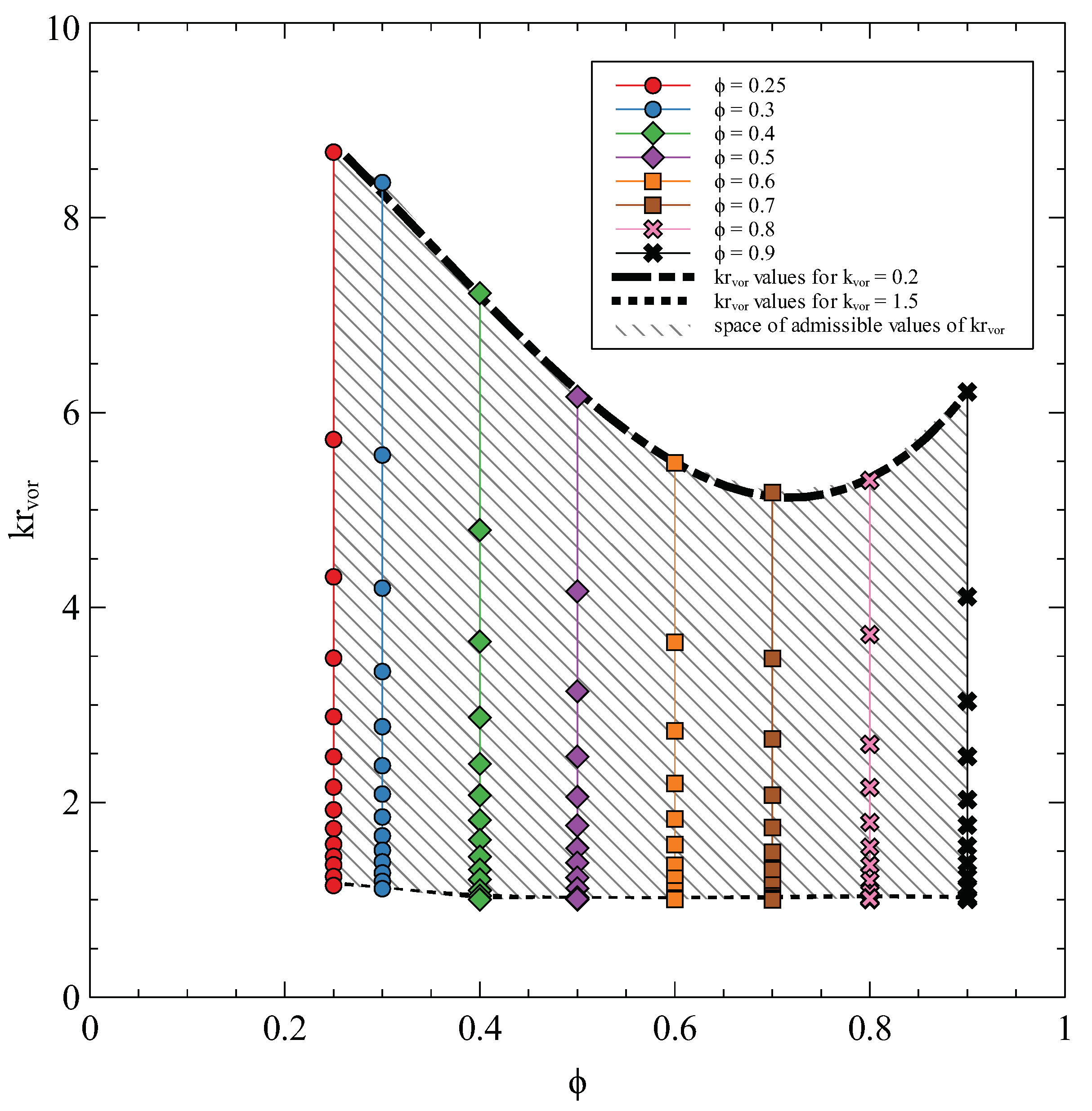
Physical solution of krvor obtained by CFD placed into the overall space of solutions.

Figure 27.
Comparison of efficiency considering fixed vortex and variable vortex size.

Figure 28.
CFF efficiency formulation.

Table 1.
Description of the loss models using streamline analysis.
| Model | Formulation | Description and Characteristics |
|---|---|---|
| Skin friction loss | Pressure loss due to friction between air, blade wall, and casing inner wall | |
| First law | First stage: pump | |
| Second law | Second stage: compressor | |
| Third law | Inner surface of casing tunnel | |
| Incidence loss | Chocks between air and blade tip at the entrance of first stage | |
| Expansion loss | Decompression of the air once it is out of the blades inter-space to the tunnel | |
| Enlargement loss | Spread of the fluid vein at the exit of the second stage toward the diffuser | |
| Re-circulation loss | Related to the existence of the vortex |
Publisher’s Note: MDPI stays neutral with regard to jurisdictional claims in published maps and institutional affiliations. |
© 2022 by the authors. Licensee MDPI, Basel, Switzerland. This article is an open access article distributed under the terms and conditions of the Creative Commons Attribution (CC BY) license (https://creativecommons.org/licenses/by/4.0/).
Share and Cite
MDPI and ACS Style
Himeur, R.M.; Khelladi, S.; Ait Chikh, M.A.; Vanaei, H.R.; Belaidi, I.; Bakir, F. Towards an Accurate Aerodynamic Performance Analysis Methodology of Cross-Flow Fans. Energies 2022, 15, 5134. https://doi.org/10.3390/en15145134
AMA Style
Himeur RM, Khelladi S, Ait Chikh MA, Vanaei HR, Belaidi I, Bakir F. Towards an Accurate Aerodynamic Performance Analysis Methodology of Cross-Flow Fans. Energies. 2022; 15(14):5134. https://doi.org/10.3390/en15145134
Chicago/Turabian StyleHimeur, Rania M., Sofiane Khelladi, Mohamed Abdessamed Ait Chikh, Hamid Reza Vanaei, Idir Belaidi, and Farid Bakir. 2022. "Towards an Accurate Aerodynamic Performance Analysis Methodology of Cross-Flow Fans" Energies 15, no. 14: 5134. https://doi.org/10.3390/en15145134
Note that from the first issue of 2016, this journal uses article numbers instead of page numbers. See further details here.