
Validation of a Method for Measuring the Position of Pick Holders on a Robotically Assisted Mining Machine’s Working Unit


Department of Mining Mechanization and Robotisation, Faculty of Mining, Safety Engineering and Industrial Automation, Silesian University of Technology, Akademicka 2, 44-100 Gliwice, Poland
*
Author to whom correspondence should be addressed.
Energies 2022, 15(1), 295; https://doi.org/10.3390/en15010295
Submission received: 22 November 2021
/
Revised: 15 December 2021
/
Accepted: 25 December 2021
/
Published: 2 January 2022
(This article belongs to the Special Issue The KOMTECH-IMTech 2021 Mining Technologies Future)
Abstract
:For effective mining, it is essential to ensure that the picks are positioned correctly on the working unit of a mining machine. This is due to the fact that the design of roadheader cutting heads/drums using computer-aided tools is based on the operating conditions of the roadheader/shearer/milling machine. The geometry of the cutting head is optimized for selected criteria by simulating the mining process using a computer. The reclaimed cutting head bodies that are utilized in production are manufactured again in the overhaul process. Ensuring that the dimensions of the cutting head bodies match the rated dimensions is labor-intensive and involves high production costs. For dimensional deviations of the cutting head bodies, it is necessary to control the position of the pick holders relative to the cutting head side surface in real time during robotic-assisted assembly. This article discusses the possibility of utilizing a stereovision system for calculating the distance between the pick holder base and the roadheader cutting head side surface at the point where the pick holder is mounted. The proposed measurement method was tested on a robotic measurement station constructed for the purpose of the study. A mathematical measurement model and procedures that allow automatic positioning of the camera system to the photographed objects, as well as acquisition and analysis of the measurement images, were developed. The proposed method was validated by using it for measuring the position of the pick holders relative to the side surface of the working unit of a mining excavating machine, focusing on its application in robotic technology. The article also includes the results observed in laboratory tests performed on the developed measurement method with an aim of determining its suitability for the metrology task under consideration.
1. Introduction
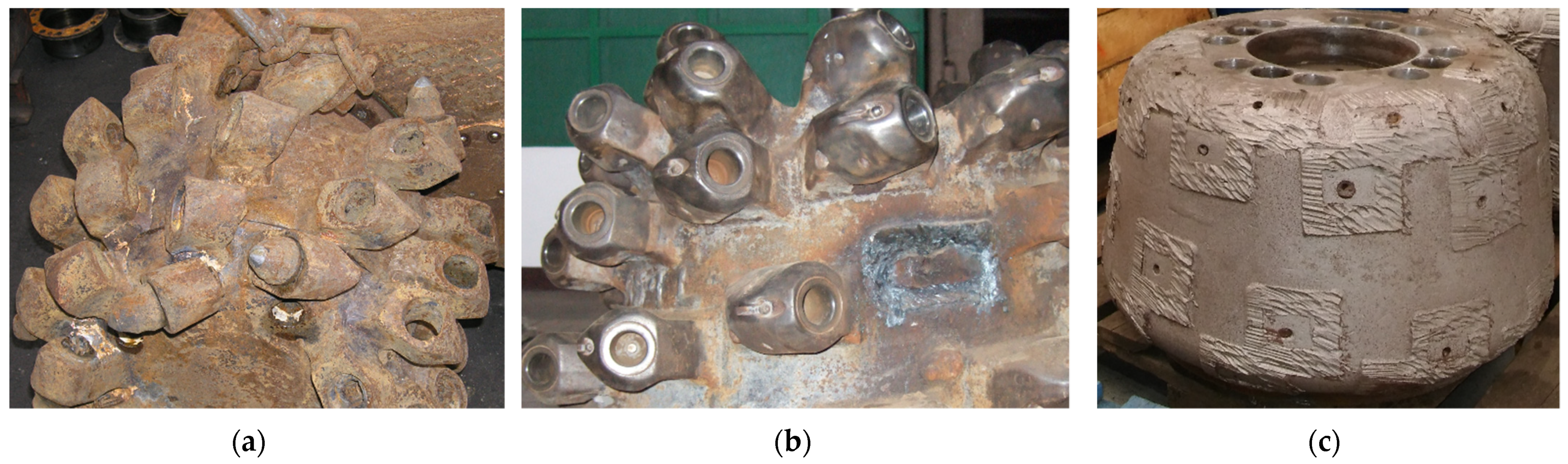
Improper positioning of picks on the cutting head negatively affects the efficiency of the mining process, increases energy consumption, and impacts the durability of key components of the cutting roadheader and cutting tools [1,2,3,4]. Excessive wear and tear of the cutting picks and inappropriate maintenance of the roadheader result in wear, cracking, and even ripping out of the pick holders. In such cases, the cutting head will lose its properties and should be replaced by a new one, as well as subjected to a reconditioning procedure by the manufacturer (Figure 1).
During the designing of pick systems, the specific conditions of roadway or tunneling excavation are taken into consideration [5,6]. Software that is specific for pick system designing with a built-in simulation module allow optimization of the stereometric parameters of the cutting head in terms of factors such as productivity, energy consumption, large output grain size, and dynamic loads [7]. To ensure that the designed pick layout meets the expectations of the users, it must be reproduced faithfully during the manufacturing process [8]. Cutting head bodies are often recovered and remanufactured in the overhaul process; therefore, their dimensions may differ from the rated dimensions. In this case, even if the robotic technology is applied in the production of cutting heads, high accuracy and repeatability of the final product are uncertain unless the pick holders are controlled and possibly adjusted during their assembly on the cutting head side surface. Adaptive controlling of the robot that positions the pick holder during installation necessitates the online measurement of the distance distribution between the base of each pick holder and the cutting head side surface at the assembly point. The use of a measurement method enables the evaluation of the weldability of pick holders, the detection of potential collisions, and the automatic correction of the position of the pick holder so that it can be welded.
In the metrology of geometric quantities, contact and non-contact methods are used [9]. Optical contactless methods are commonly used in robotic technologies. These include, among others, the two-image photogrammetric method [10]. Optical methods are characterized by high measurement speed, as they are based on the processing of data recorded by optoelectronic transducers. They are used in industries such as automotive, glass, pharmaceutical and food, or printing houses. Vision systems of varying complexity are used in quality control, automation of technological processes, and reverse engineering [11,12].
In this work, an automatic measurement method was developed to determine the distance distribution between the pick holder base and the cutting head side surface during the positioning of the pick holder at the assembly station. This is a contactless method developed specifically for the metrology task under consideration. Indeed, vision systems are widely used in robotics for different applications, such as quality control, distance measurement, and object inspection [13,14,15].
The article briefly discusses the algorithm of the proposed measurement method and presents a mathematical model of the measurement. The present work aimed to validate the proposed measurement method to the metrology requirements associated with the technical conditions of the manufacturing of a mining machine’s working faces. The article also describes the configuration of the test bench and presents the results observed in the laboratory tests conducted in the study. The final section presents sample measurement results obtained by applying the developed method.
2. Characteristics of the Proposed Method and Measurement Model
Robot-assisted positioning of the pick holders on the cutting head side surface is per-formed based on the data obtained from dedicated design-supporting software [16]. One such software is Kreon (Department of Mining Mechanization and Robotisation, Silesian University of Technology, Gliwice, Poland) which was developed by the Department of Mining Mechanization and Robotisation of the Faculty of Mining, Safety Engineering and Industrial Automation of the Silesian University of Technology [17,18]. When off-line programming of industrial robots is carried out using computer tools such as Kuka.SimPro software (KUKA AG, Augsburg, Germany), information about the position and spatial orientation of a specific pick holder is converted into positioning instructions that control the robot’s movements on the assembly station.
To measure the distance between the base of a given pick holder and the cutting head side surface at the location of attachment of the pick holder, the arm of the pick holder-positioning robot stops at a certain distance when approaching the target position to photograph the pick holder’s installation place and acquire measurement images. Two cameras working in a convergent manner are used for image acquisition. The cameras along with the projection device constitute an active stereovision measurement system [19,20,21]. The measurement system is controlled (on/off projection laser, acquisition and processing of measurement images) through a program that controls the operation of two robots—one positioning the pick holders and one positioning the vision system.
The idea behind the measurement is to determine the spatial position of a grid of points projected onto the cutting head side surface with the use of a laser fitted with a diffraction grid (51 × 51 points). This projection device is mounted on the robotic arm that positions the pick holder [22,23]. A two-image method (stereophotogrammetry) is used for determining the spatial position. The density of the marker grid projected onto the reconstructed side surface was selected in such a way as to allow, on the one hand, sufficient accuracy in reproducing its shape (for the presented task) [24] and, on the other hand, reducing the amount of measurement data and thus eliminating the redundancy of the processed information, as is the case of, for example, in scanning. An enormous amount of redundant data would complicate the measurement procedure as well as increase the lead time, which would affect the timing of the robotic station waiting for the measurement result.
2.1. Test Bench
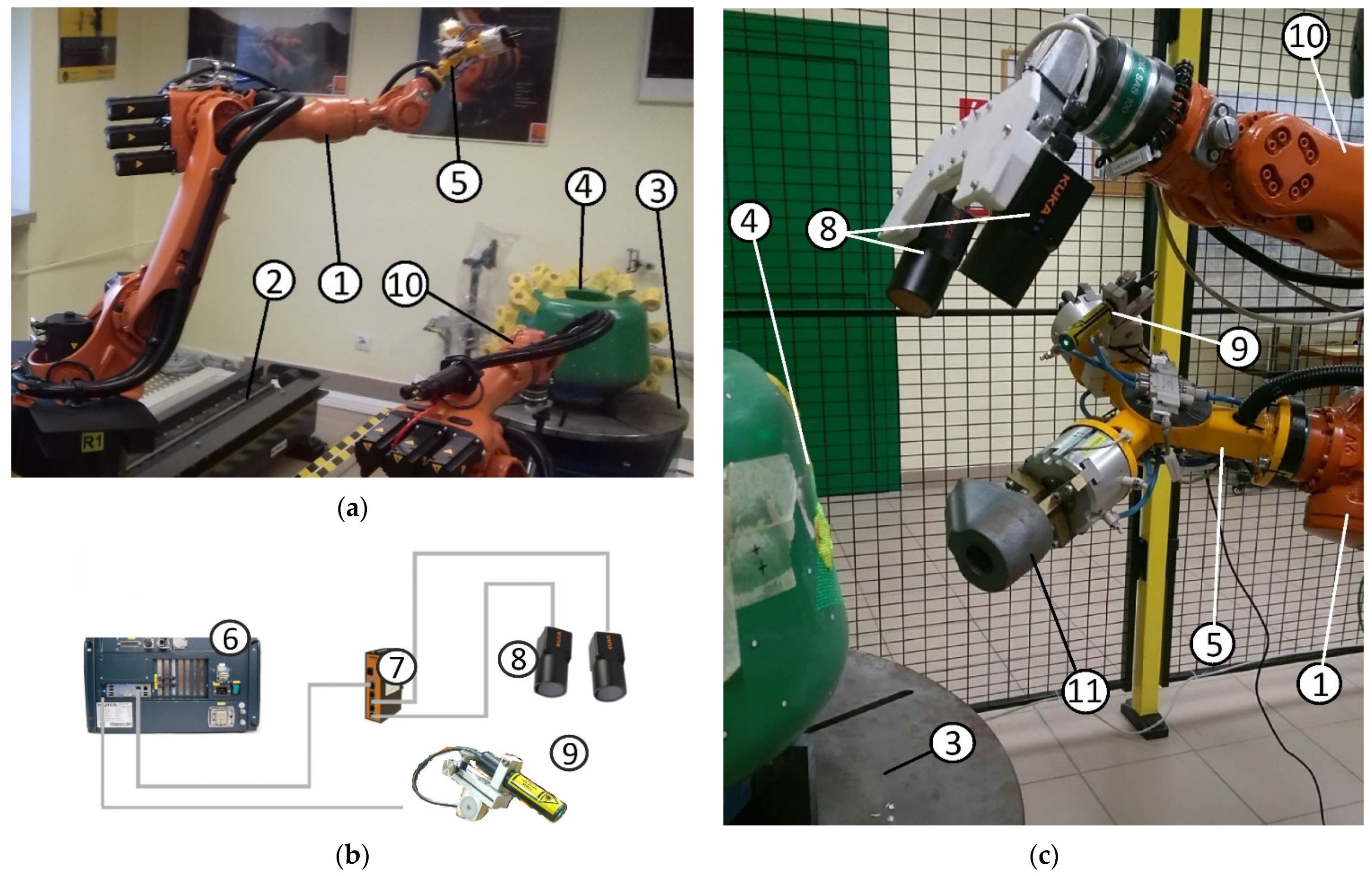
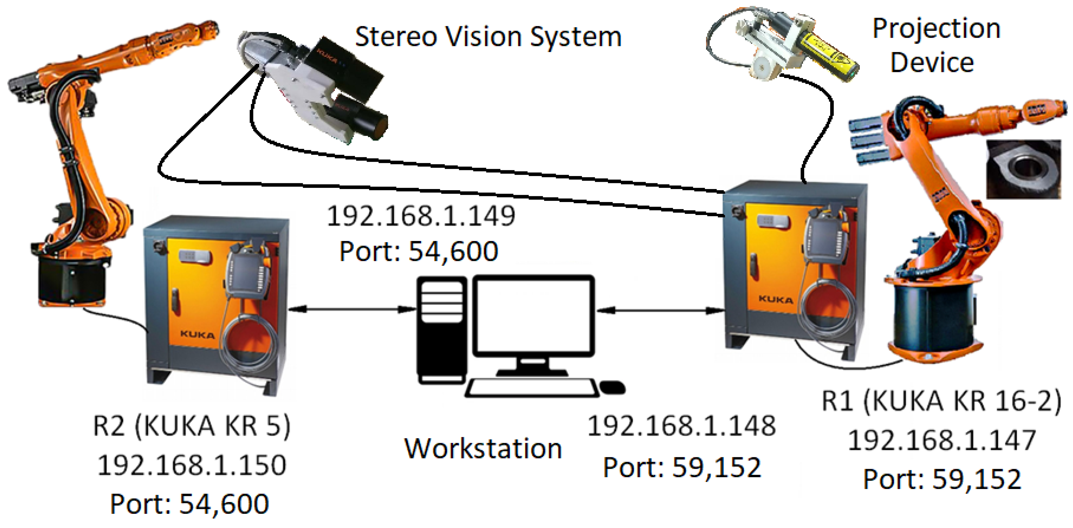
The developed measurement method was evaluated on a measuring bench in the Robotics Laboratory of the Department of Mining Mechanization and Robotisation of the Faculty of Mining, Safety Engineering and Industrial Automation of the Silesian University of Technology (Figure 2). The test bench was equipped with two KUKA industrial robots: KR 16-2 and KR 5. The KR 16-2 robot consists of a gripper for picking up and positioning the pick holders from the tray and positioning the projection device. While a given pick holder is being positioned, information about the position of the tool coordinate system is transmitted to the workstation (Figure 3) which is connected to the robots via Ethernet [25,26]. Communication between the workstation and the control system of both KR 16-2 and KR 5 robots occurs via a client–server architecture (Figure 4). The workstation determines the position of the robot that positions the vision system. The information about the position is sent to the KR 5 robot, which moves the vision system into an appropriate position. Once the projection device is turned on, the measurement images are acquired. The images are downloaded, processed, and analyzed on a workstation in the Matlab environment with Image Processing Toolbox and Computer Vision Toolbox libraries installed. The measurements indicate the distance distribution between the cutting head side surface and the pick holder base. Table 1 provides the details of the cameras and lenses used to build the video system.
2.2. Processing and Analysis of Measurement Images
The recorded measurement points are extracted from segmented images by applying morphological operations and binarization with adaptive thresholding [27,28]. Thus, markers are extracted from a pair of measurement images as regions with a value of 1 in the binary image. The position of these regions in the images is described by (x, y) coordinates expressed in pixels.
The Matlab (MathWorks, Natick, MA, USA) triangulate function is used to obtain the spatial coordinates of a given point in the reference system associated with the left camera of the vision system, based on the position of the point (measurement marker) on a pair of images (Figure 5a) [29,30,31,32]. The resulting grid of points represents the cutting head side surface at the point where the pick holder is mounted. To determine the coordinates of these points in the reference system associated with the pick holder base, a transformation must be performed for each point. This will result in a distance distribution of the points of the cutting head side surface from the pick holder base (Figure 5b) [33]. The transformation is described by homogeneous matrices (1) and (2) (Figure 5c):
The components of the measuring point direction vector in the coordinate system of the robot tool are as follows:
where:
αU is the angle between the optical axes of the cameras and the ZT axis of the coordinate systems related to the vision system,
lX is the distance between the origin of the coordinate system associated with the optical system of the left camera and the origin of the XTYTZT coordinate system of the cameras along the XT axis,
lZ is the distance between the origin of the XTYTZT coordinate system and the origin of the coordinate system of the left camera measured along the ZT axis,
φDP, γDP, and αDP are the angles that define the position of the vision system (XTYTZT) relative to the pick holder base (XPYPZP), and
lL and lA are the distances that define the position of the vision system (XTYTZT) relative to the pick holder base (XPYPZP).
3. Calibration of the Measuring System
The developed measurement system was calibrated in two stages. The first stage involved the calibration of the stereovision system, while the second involved determination of the values of the binding points between the vision system and the robot on the arm of which the vision system is installed. This stage is critical for determining the actual position and alignment of the vision system in space relative to the photographed cutting head side surface mounted on the positioner face, to which the robot base’s coordinate system is related [33].
3.1. Camera Calibration
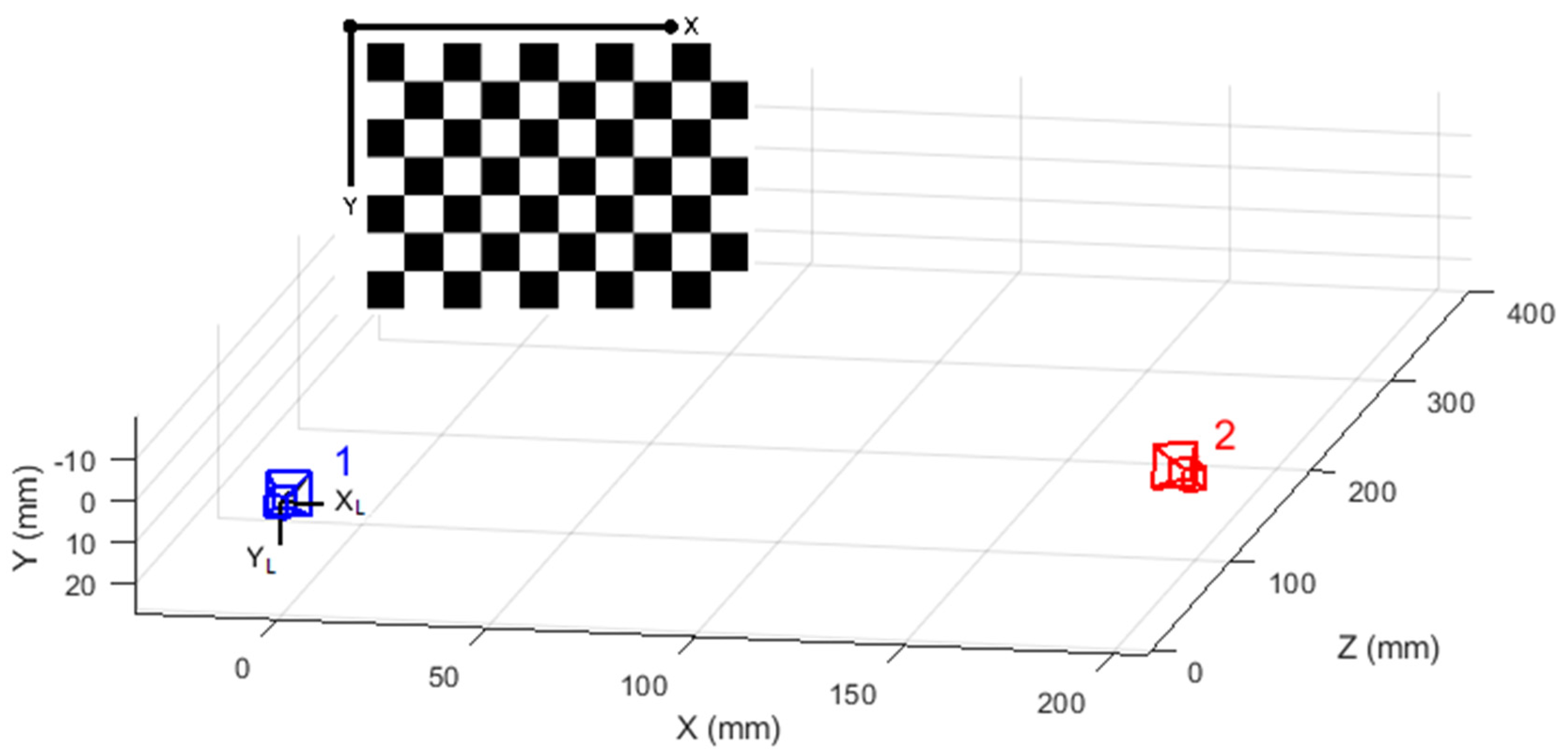
The measurement process begins with the calibration of the vision system, the purpose of which is to estimate the values of the internal and external camera parameters [34]. The internal parameters define the optical properties of the lens, and their radial and tangential distortion (Table 2). In addition, the coordinates of the image center (principal point) and the projection center (a focal point of the optical system) are determined. In turn, the external parameters describe the shift and rotation of the coordinate systems of the cameras relative to the coordinate system associated with the observed scene as well as the relationship between the cameras (Table 3). The developed measurement method made use of the default camera calibration method provided by the Matlab environment. The cameras were calibrated by taking 15 images at different positions relative to the calibration table (Figure 6). The calibration error of the camera system is less than 0.5 pixels in Matlab [35]. The calibration of the stereovision system allowed its reference system to be hooked to the focal point of the left camera’s optical system, with one of its axes coinciding with the optical axis of the lens.
3.2. Determination of the Parameter Values for the Transformation of the Coordinate System of the Robot Tool to the Coordinate System of the Measurement System’s Left Camera
To determine the position of the OS measurement point in the base system with a known position described by the leading vector rOB, the values of the parameter describing the transformation of the robot tool coordinate system (XTYTZT) to the coordinate system of the developed measurement system’s left camera (XLYLZL) should be determined (Figure 7). The acquisition of measurement images and their processing using the libraries of the Matlab environment enabled the determination of the position of the considered measurement point in the coordinate system of the stereovision system’s left camera. The position of the OS point in the left camera coordinate system is described by the leading vector rOK. Therefore, based on the position of the TCP point of the robot, on the arm of which the stereovision system is mounted, and the orientation of the axis of the tool coordinate system hooked at this point (XTYTZT) relative to the axis of the robot base coordinate system (XBYBZB), the direction vector of the OS point in the XBYBZB coordinate system can be calculated as:
where the direction vectors of the individual characteristic points consist of the following components:
while the complex rotation matrices are the product of the rotation matrices about the Z, Y, and X axes by the corresponding angles:
where:
is the direction vector of the OS measurement point in the robot base coordinate system XBYBZB,
is the direction vector of the central point of the robot tool in the XBYBZB coordinate system,
is the direction vector of the projection center (focal point) of the stereovision system’s left camera in the robot tool coordinate system XTYTZT,
is the direction vector of the OS measurement point in the left camera’s coordinate system XLYLZL,
is the complex rotation matrix of the XTYTZT coordinate system in the XBYBZB coordinate system, and
is the complex rotation matrix of the left camera coordinate system in the XTYTZT coordinate system.
The measured parameters describe the translation of the robot tool coordinate system to the KL point (focal point of the optical system) of the left camera in the form of components of the translation vector in the direction of the XT, YT, and ZT axes (K1.X, K1.Y, and K1.Z), and also describe the rotation of this coordinate system in the form of angles of rotation about the axes ZT, YT, and XT (K1.A, K1.B, and K1.C):
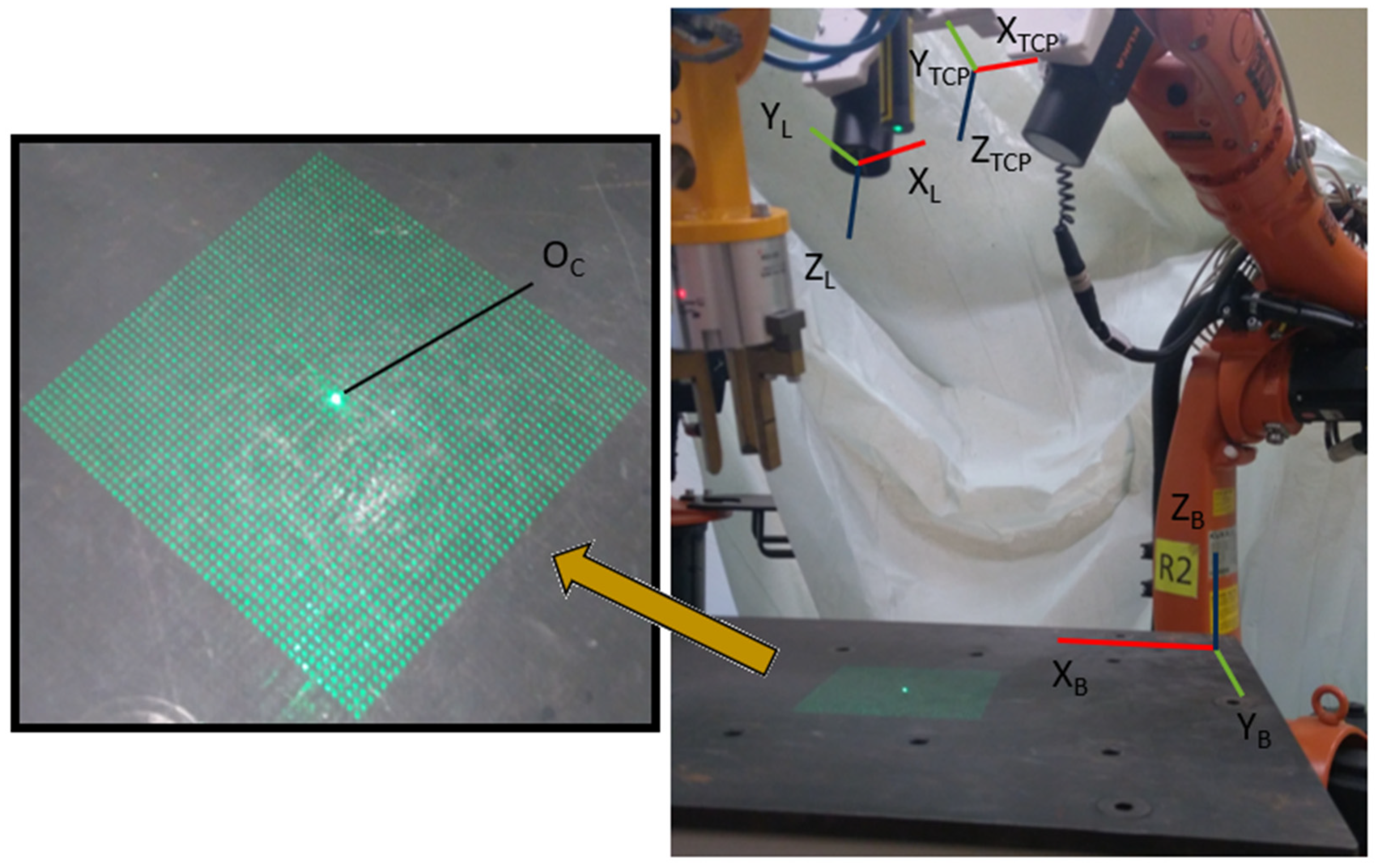
Preliminary tests revealed that the adoption of parameter values (11) based on the CAD model of the developed stereovision system does not result in the desired accuracy of the obtained measurement results. This is due to certain incompatibilities between the geometry of the measurement system design and the CAD model (design). The bracket (carrier element), to which the cameras of the developed measurement system are attached, was created using the powder-based selective heat sintering three-dimensional (3D) printing technology, a process that leads to slight deformation of the printed parts and dimensional deviations (shrinkage). Thus, during the second calibration stage, the parameter values (11) were determined experimentally by measuring the position of the laser grid points projected onto the projection plane—the robot base plane XBYB (Figure 8). For this purpose, a grid of points of known dimensions (pattern) was photographed by changing the settings of the video system so that as many points as possible were within the field of view of both cameras.
To synchronize the pattern measurement points with the points recorded during measurement with the calibrated stereovision system in the robot base coordinate system, the set of parameters (11) was supplemented by three additional unknown variables, namely the displacement of the central point OC of the pattern (clearly distinguished in the measurement images by its brightness) in the direction of the axis of the robot base coordinate system: Δx, Δy, and Δz. Starting with Equation (4), the problem taken into consideration is thus reduced to determining the values of the following nine unknowns:
This requires the construction of a system of nine algebraic equations that define the relationships between the direction vectors of three selected measurement points in the robot base coordinate system and the coordinate system of the measurement system’s left camera. These are nonlinear equations that must be solved through numerical (iterative) methods. Furthermore, there is the issue of selecting the measurement points for the considered coordinates.
However, the values of the parameters were determined by using a different approach. To eliminate the effect of the camera set to the photographed object (pattern), which results in a different distribution of measurement points recorded on stereograms, measurement data from four measurement series performed for different positions of the robot tool (different stereovision system settings) were used. In each series, approximately 1500 measurement points were recorded. As a result, the topic under discussion is reduced to the problem of minimizing a multivariate objective function. The values of (12) were determined by considering the following three objective functions:
while:
where:
αHVi is the inclination angle of the i-th segment with ends at OSi and OSj points to the laser projection plane of the point grid (XBYB plane),
are the average values of deviations of the coordinates of measurement points in the direction of individual axes of the robot base coordinate system XBYBZB,
xOBi, yOBi, and zOBi are the coordinates of the i-th measurement point obtained from the measurement with the developed stereovision system (for i = 1, 2, …, n),
, , and are the coordinates of the i-th pattern point in the XBYBZB coordinate system (for i = 1, 2, …, n), and n is the number of measurement points considered.
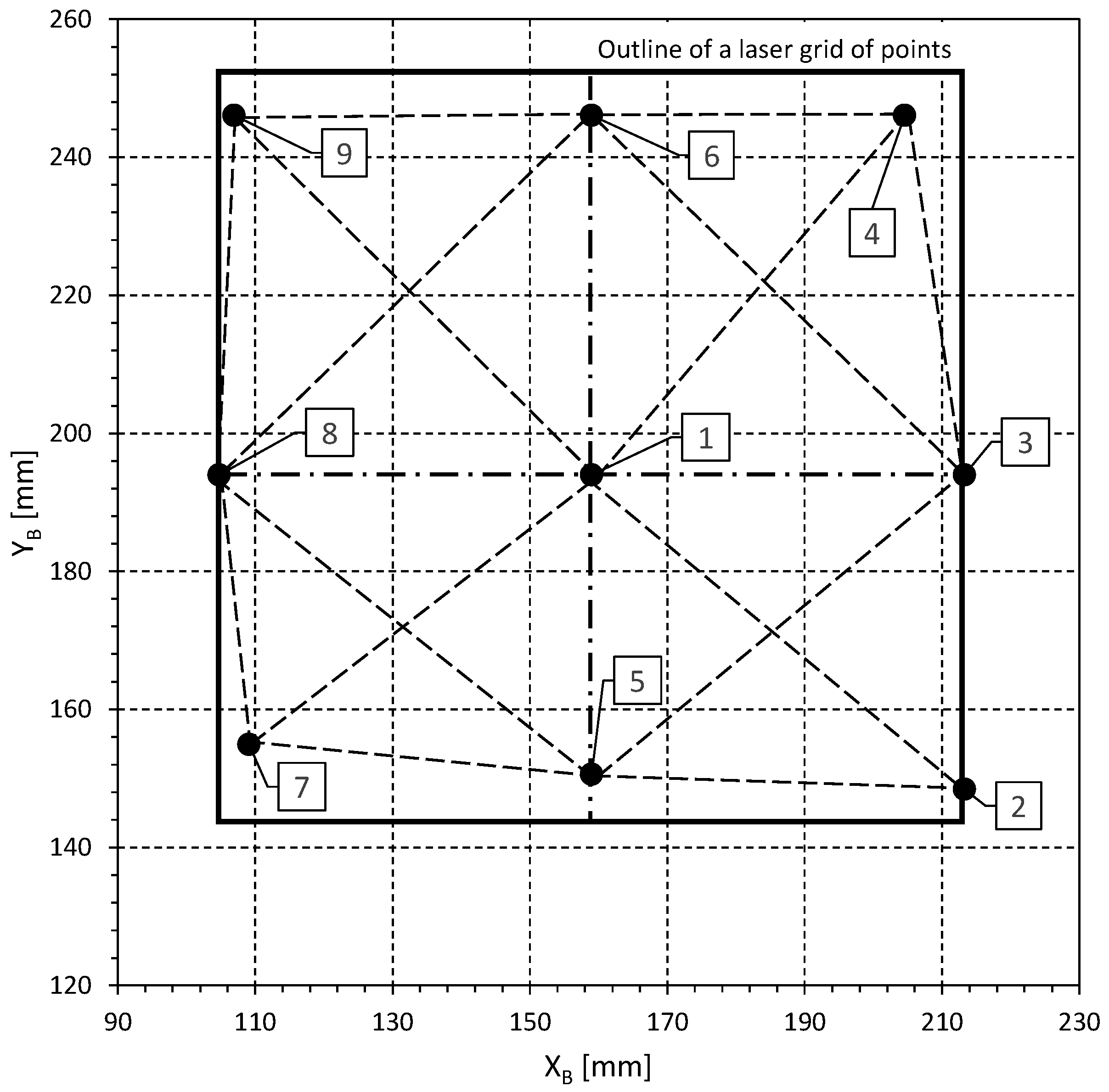
The minimum of the objective functions (13)–(15) was searched for the nine characteristic measurement points taken from the measurement in each of the four measurement series (when measurement photographs were acquired from four different photographic stands). Thus, the calibration dataset included the spatial coordinate values of 4 × 9 measurement points in the robot base coordinate system (XBYBZB). The same measurement points, i.e., the laser grid’s center point (point 1), extreme points on the grid’s mutually perpendicular axes (points 3, 8, and 5, 6), and points in the grid’s corners (points 2, 4, 7, and 9), were considered in all cases (Figure 9).
As shown in Equations (13)–(15), there is an association between the values of the parameters describing the transformation of the robot tool coordinate system to the left camera coordinate system. On the one hand, such an association will allow minimization of the inclination angle of the segments determined by the considered αHV measurement points (dashed lines and point lines in Figure 9), and thus their arrangement in the plane parallel to the XBYB plane. On the other hand, the mean error of these points’ coordinates (ε) in the direction of the robot base coordinate system axis is minimized to ensure that they are as close as possible to the reference points. For the first analyzed objective function (F1), the maximum value from the value set of the αHV angle is minimized, while for the function F2 the average value of the αHV angle is minimized and for F3 the standard deviation, which indicates the variability of the αHV angle around its average value, is minimized. For the nine measurement points considered, there are 20 sections for which the αHV angle values are calculated from Equation (16) (Table 4).
Due to the nonlinear nature and complexity of the analyzed objective functions in the domain determined by the set of studied arguments, their minimization was carried out using numerical methods, such as the advanced nonlinear Levenberg–Marquardt algorithm (LMA) which is used for solving nonlinear parameter estimation problems [36,37]. This algorithm works based on a hybrid technique that combines the Gauss–Newton method and the greatest slope method to obtain an optimal solution [38]. This algorithm belongs to the iterative algorithms group, in which the unknown parameter vector P at k+1 iteration steps is defined by the relation [39]:
where:
J(P) is the Jacobian matrix,
I is a unitary matrix,
ζk is the scalar parameter that varies in the iteration process, and
ε(P) is the error vector in successive iteration steps.
The convergence and efficiency of LMA are highly dependent on the selection of the starting point [40]. If the algorithm is not selected carefully, it can be divergent [39]. Compared with the other methods used for finding the function minimum, the Levenberg–Marquardt algorithm is more advantageous due to its fast convergence [41].
Considering the possibility of the existence of multiple local minima of the analyzed functions, the effect of the starting point on the results obtained for the iterative search for the minimum by LMA was studied. The variation ranges of the initial values of the determined parameters are summarized in Table 5. The search area for starting values for the minimization process was selected based on the geometry of the developed measurement system assumed from the CAD model (design). The search space for the starting values of the parameters describing the transformation of the robot tool coordinate system to the left camera coordinate system also included the variation intervals of the laser grid center point offset (pattern) in the direction of XB and YB axes (Δx and Δy, respectively).
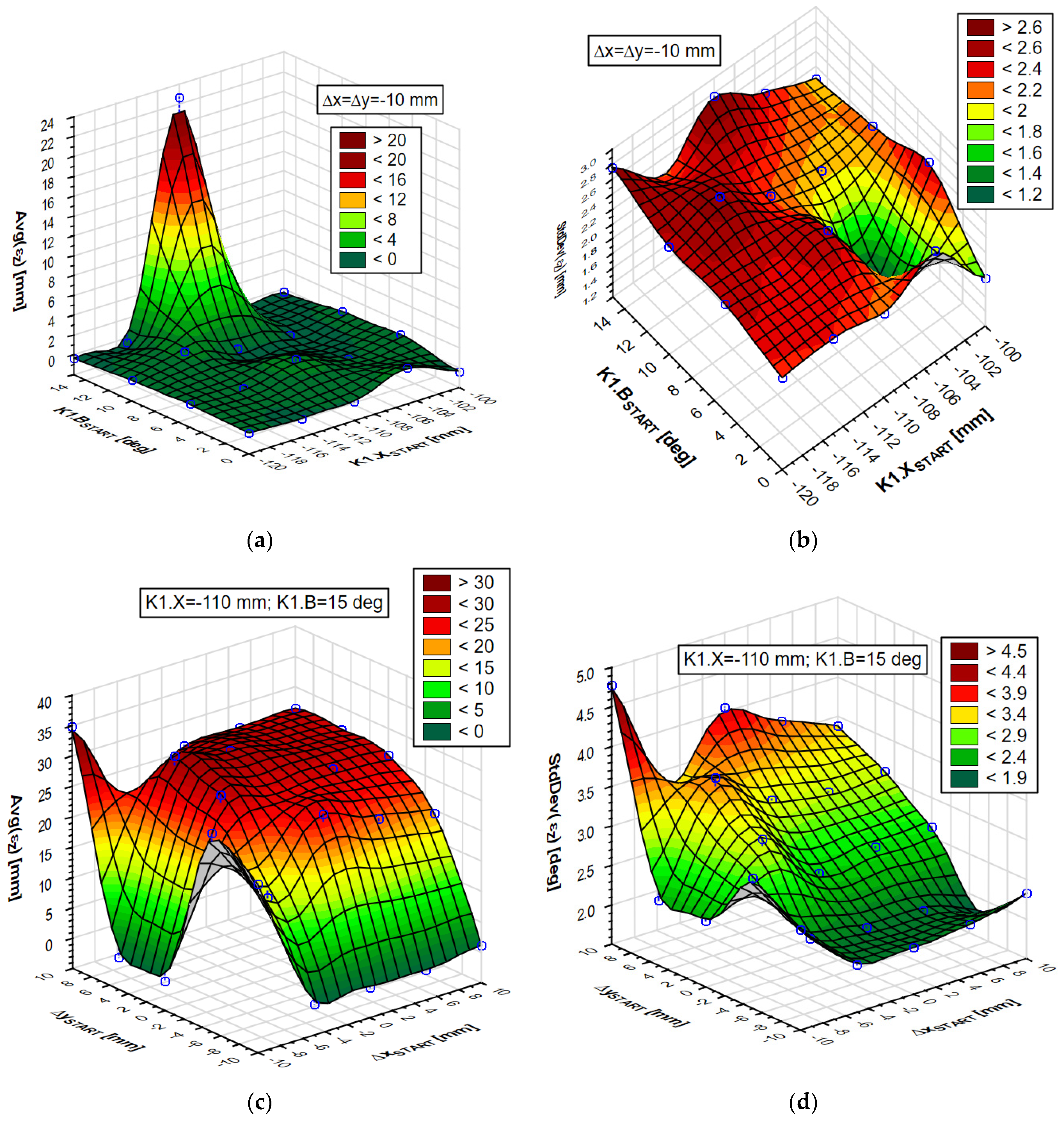
As illustrated in Figure 10, the effect of the minimization of the adopted objective functions is significantly influenced by the initial values of the sought parameters. The average value and the standard deviation of the coordinate deviation of the measurement points in the direction of the ZB axis—marked respectively—were used as indicators for evaluating the results of the search for the minimum of the objective function: Avg(εZ) and StdDev(εZ), thus in the direction of the depth of the measurement space. These deviations were determined for the nine measurement points and the four measurement series taken into consideration. For example, for Δx = Δy = −10 mm, within the studied variation range of the initial parameter values (K1.X and K1.B), the average value of deviation varies from −0.45 mm up to 22.67 mm (Figure 10a). The standard deviation of the z coordinate of the measurement points from the standard values varies between 1.08 and 2.76 mm (Figure 10b). The functions investigated here have local maxima and minima, which indicates that the association of the starting values of the determined parameters can be selected in such a way that the position error of the measured points to the corresponding standard points is minimized. The effect of the Δx and Δy shift of the laser grid is even higher (Figure 10c,d). For example, for K1.X = −110 mm and K1.B = 15°, in the measured variation range of Δx and Δy, the average deviation of the z coordinate of the measurement points varies between −0.18 and as much as 34.88 mm. In turn, the values of standard deviation of this parameter vary between 1.79 and 4.78 mm.
As described above, for all three tested objective functions (F1, F2, and F3), extensive computer analyses were performed to determine the initial values of the following:
- -
- the parameters binding the robot tool coordinate system with the coordinate system of the measurement system’s left camera; and
- -
- the displacement of the center point of the pattern (laser grid of points) relative to the origin of the robot base coordinate system.
To select the best association of the initial values of the above parameters, the following were evaluated:
- -
- the average value of deviations of the z coordinate values of the measurement points, i.e., Avg(εZ); and
- -
- the standard deviation of the distribution of the deviations of the z coordinate values, i.e., StdDev(εZ).
These values were determined after calculating the spatial coordinates of measurement points for the parameters describing the transformation of the robot tool coordinate system to the left camera coordinate system determined while minimizing the adopted objective functions.
The abovementioned statistics are the basic measurements of the value distribution of the studied characteristic (εZ deviation). In this case, the first of these indicates the distance between the measurement points and the projection plane of the pattern (z = 0). The second is a measure of the distribution variability of these distances, indicating the scatter of the measurement points in the considered direction.
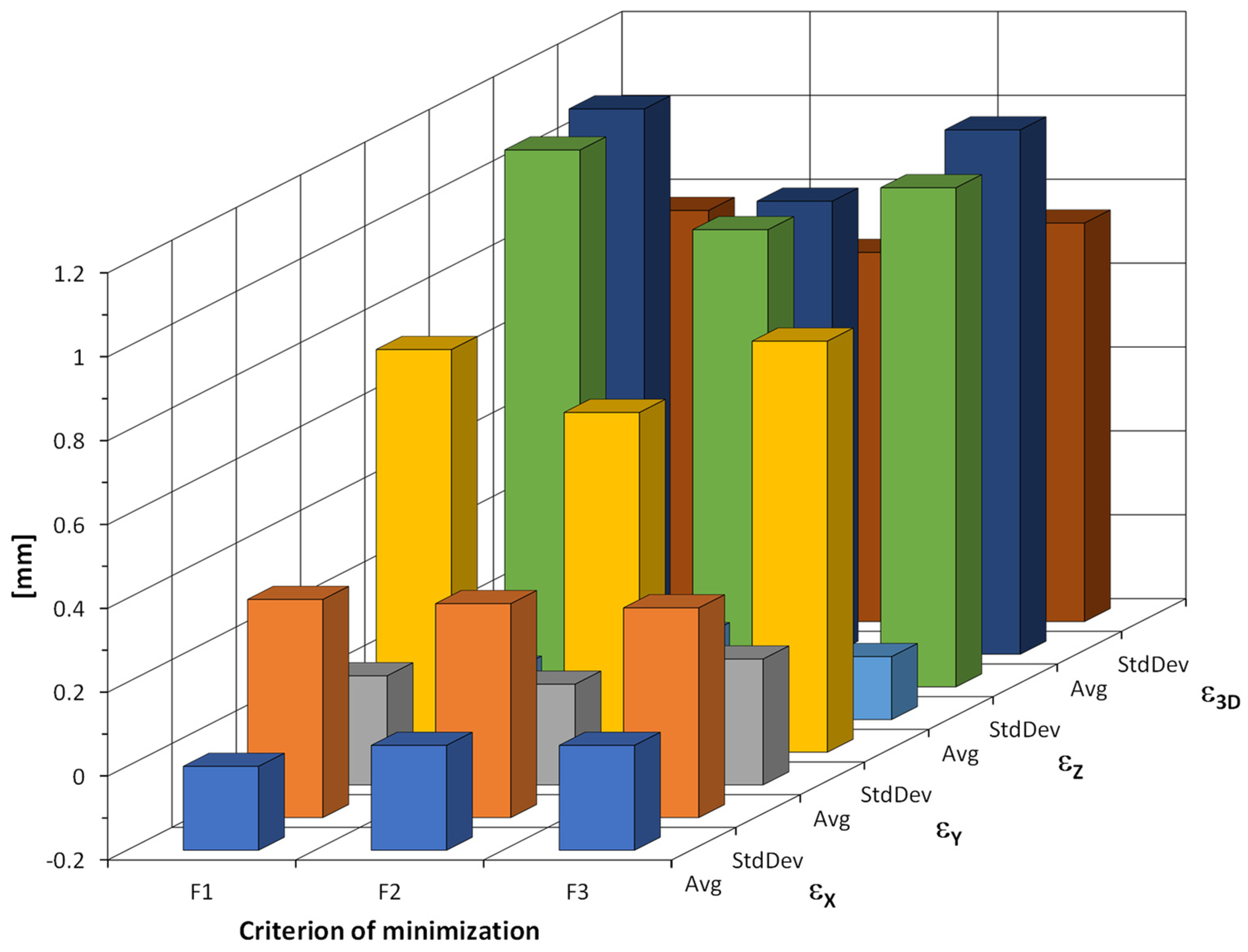
Of all the combinations of initial values of the studied parameters, the cases characterized by the smallest average value and standard deviation of the εZ deviation distribution for all 36 measurement data were selected for each of the studied objective functions. The results of the minimization process of the studied objective functions are presented in Figure 11. In addition to the above statistics for evaluating the objective function minimization results, the graph also includes the statistics for the other two coordinates of the measurement points (εX and εY) and the spatial deviation (ε3D), which is the geometric sum of the deviations along the XB, YB, and ZB axes. As can be seen from the figure, the average value of the εZ deviation ranges between –0.08 and 0 mm, while the standard deviation of the distribution of these deviations ranges between 0.89 and 1.08 mm. For the other two coordinates, however, the values of the analyzed statistics fall within the limits:
- -
- x-coordinate: average value Avg(εX) ranges between 0 and 0.05 mm, and standard deviation StdDev(εX) between 0.30 and 0.32 mm;
- -
- y-coordinate: average value Avg(εY) ranges between 0.04 and 0.10 mm, and standard deviation StdDev(εY) between 0.31 and 0.78 mm.
On the other hand, for spatial deviation (ε3D), the average value ranges between 0.88 and 1.10 mm and the standard deviation between 0.68 and 0.78 mm.
The described distributions of measurement point coordinate deviations to the pattern were obtained for the parameters defining the transformation of the robot tool coordinate system to the left camera coordinate system of the measurement system and for the correction of the laser grid focal point position of the points (pattern), which were determined during the minimization of the studied objective functions (Figure 12).
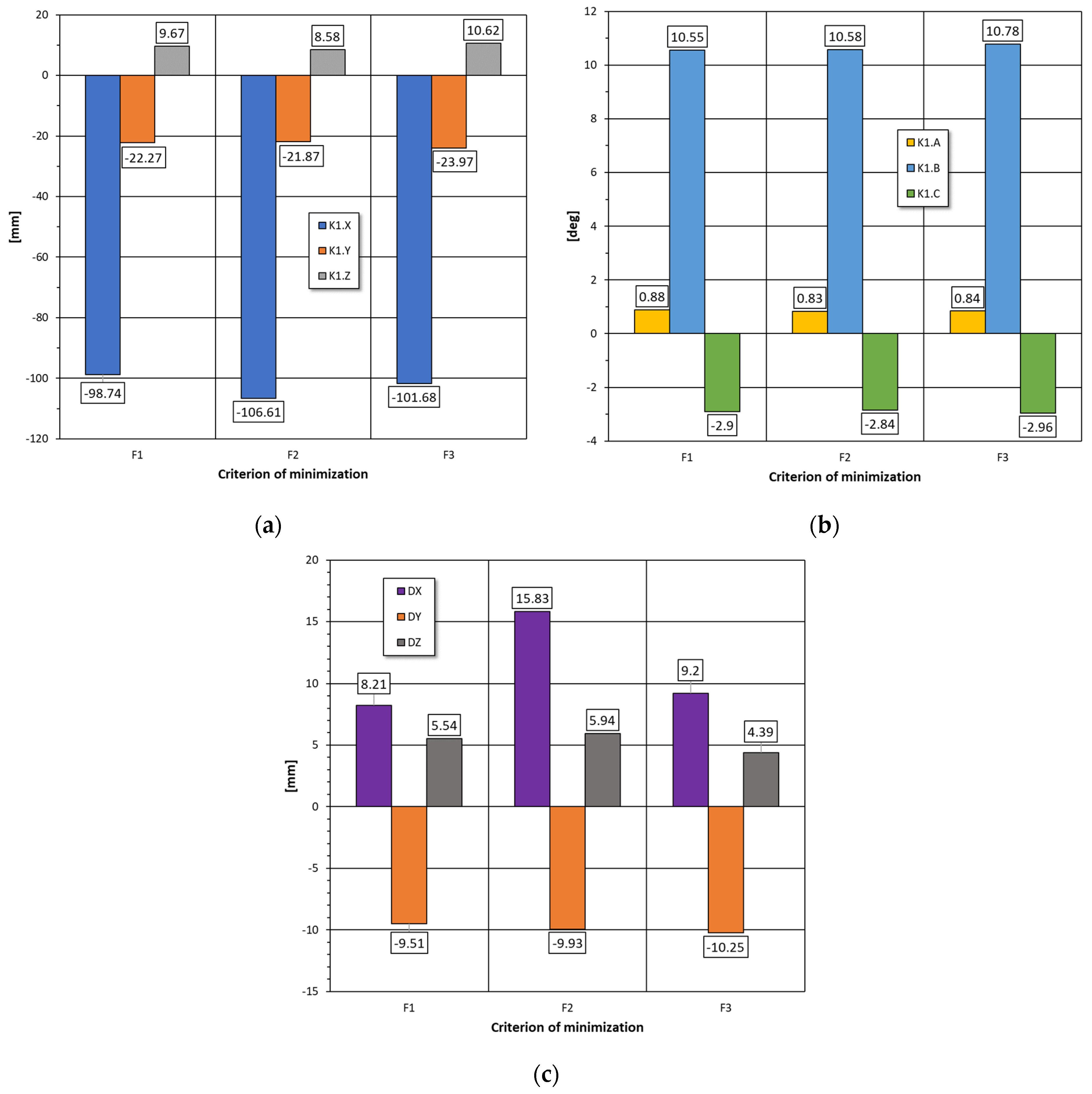
Depending on the objective function considered, the values of the parameters that bind the measurement system’s left camera to the robot tool coordinate system vary to a greater or a lesser extent (Figure 12a,b). These differences, which amount to approximately 8 mm, are particularly applicable to the translation vector component K1.X. In the case of the other components of this vector, the differences vary by ~2 mm. For the angles of rotation of the robot tool coordinate system to achieve the orientation of the left camera coordinate system, the difference is much smaller and less than 0.2°. The best possible matching of measurement points to the pattern is ensured by a correction of its location (offset) in the robot base coordinate system. The displacements in the direction of the YB axis for individual objective functions are at the level of Δy ≈ −10 mm (between −9.51 and −10.25 mm) (Figure 12c). The correction of the pattern position in the direction of the ZB axis is on average Δz ≈ 5.5 mm (between 4.39 and 5.94 mm). On the other hand, the correction in the direction of the XB (Δx) axis ranges between 8.21 and 15.83 mm, depending on the form of the minimized target function. Accordingly, this correction is characterized by the greatest variability based on the objective function considered in the minimization process.
The analysis of the results presented in Figure 11 indicated that the best results were obtained for the set of values of the parameters that were determined in the minimization process of the F2 function. The average value of the εZ-deviation distribution, in this case, was zero, and the standard deviation was 0.89 mm. The average values and the standard deviation of the deviation distribution of the other two coordinates of the measurement points were εX = 0.05 and 0.31 mm and εY = 0.04 and 0.61 mm, respectively. Conversely, the average value and standard deviation of the ε3D spatial deviations were found to be 0.88 and 0.68 mm, respectively. It should also be noted that the value of the translation vector component K1.X = −106.61 mm determined for this case was the closest to the value predicted while designing the measuring system (−105 mm).
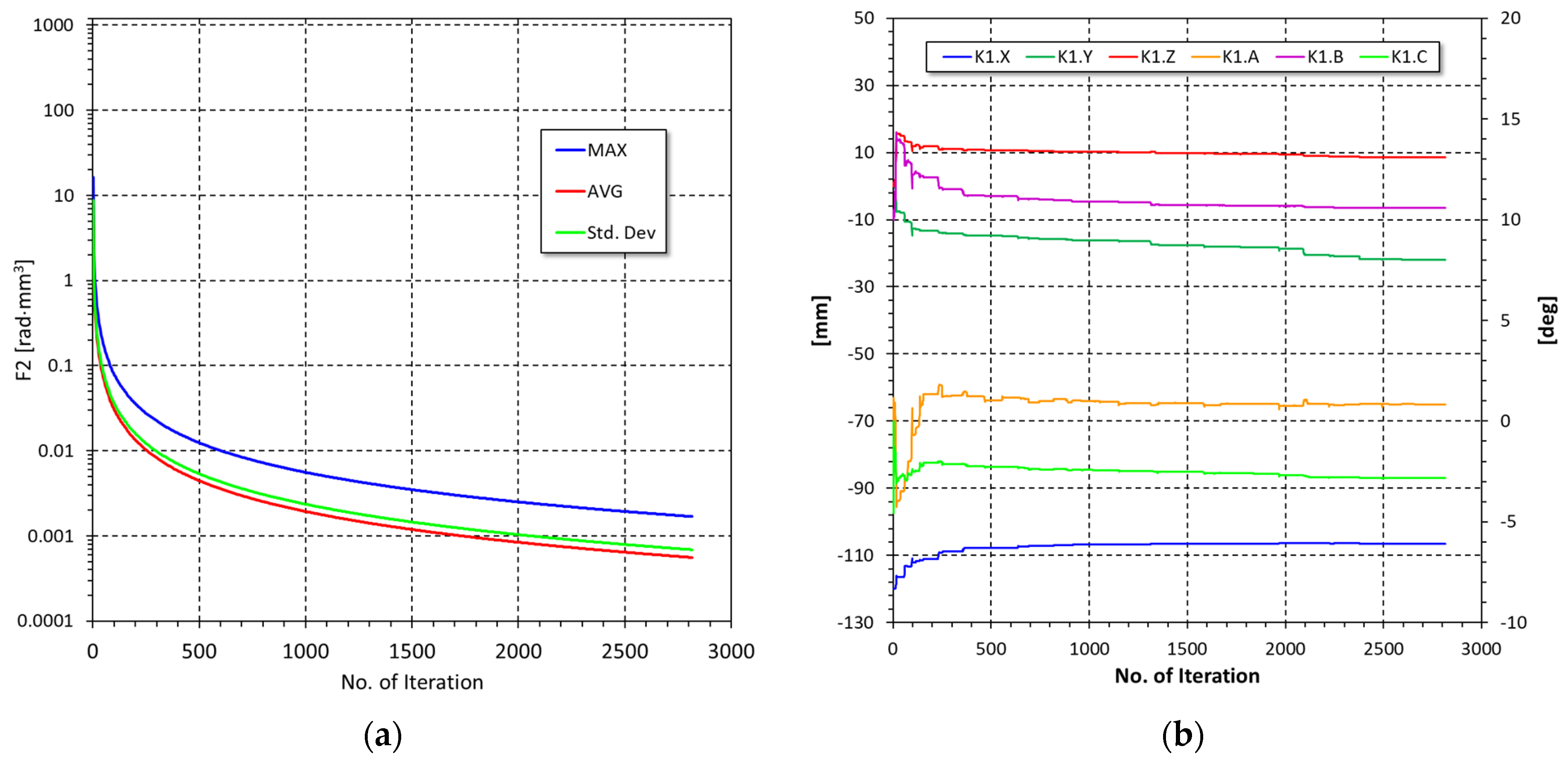
The process of minimization of the objective function F2 in successive iterations is described in Figure 13. A total of 2815 iterations were taken by the process to reach the minimum of the tested function. As can be seen in the figure, the minimization process showed the greatest convergence during the first 300 iterations (Figure 13a), whereas in subsequent iterations, the decrease in the value of the objective function successively declined, asymptotically reaching the threshold value resulting from the assumed accuracy of the minimization process. In the subsequent iterations, the sets of values of the sought parameters characterizing the left camera position in the robot tool coordinate system (Figure 13b) as well as corrections to the pattern position in the robot base system were determined.
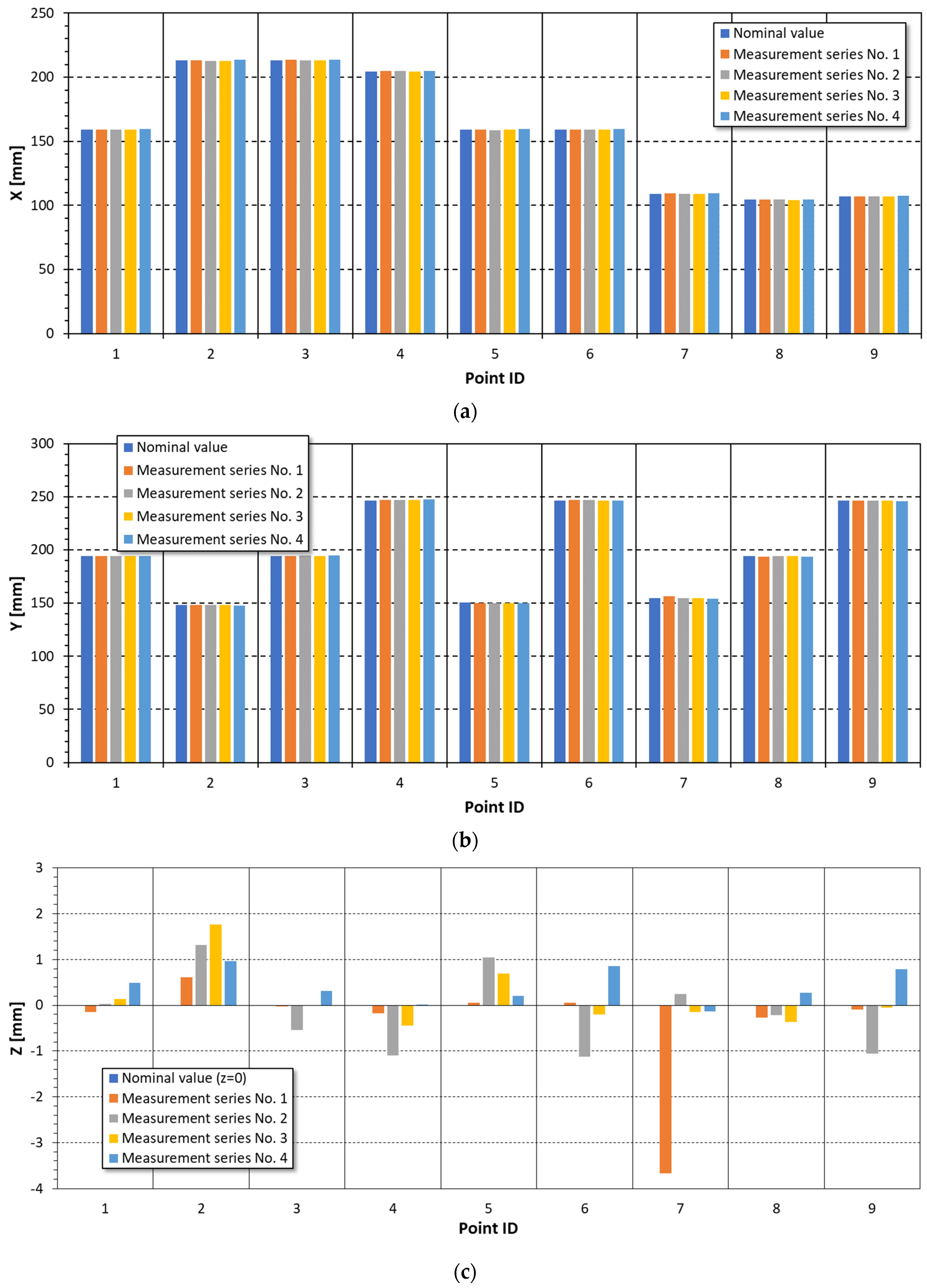
The values of coordinates of the nine measurement points measured in individual measurement series showed some differences (Figure 14). This was particularly true in the case of for the z coordinate, the value of which oscillated around zero (nominal value) (Figure 14c). However, after introducing the determined corrections of the standard position, the deviations of the measurement point coordinates remained within the limits: εX = ±0.56 mm; εY = −0.89 to +1.55 mm, and εZ = −3.67 to +1.76 mm. The largest error was noted for the measurement of point 7 in measurement series 1. This could be probably due to the erroneous identification of the position of this point on the measurement images, leading to an error in the determination of its spatial position in the arrangement of the measurement system’s left camera.
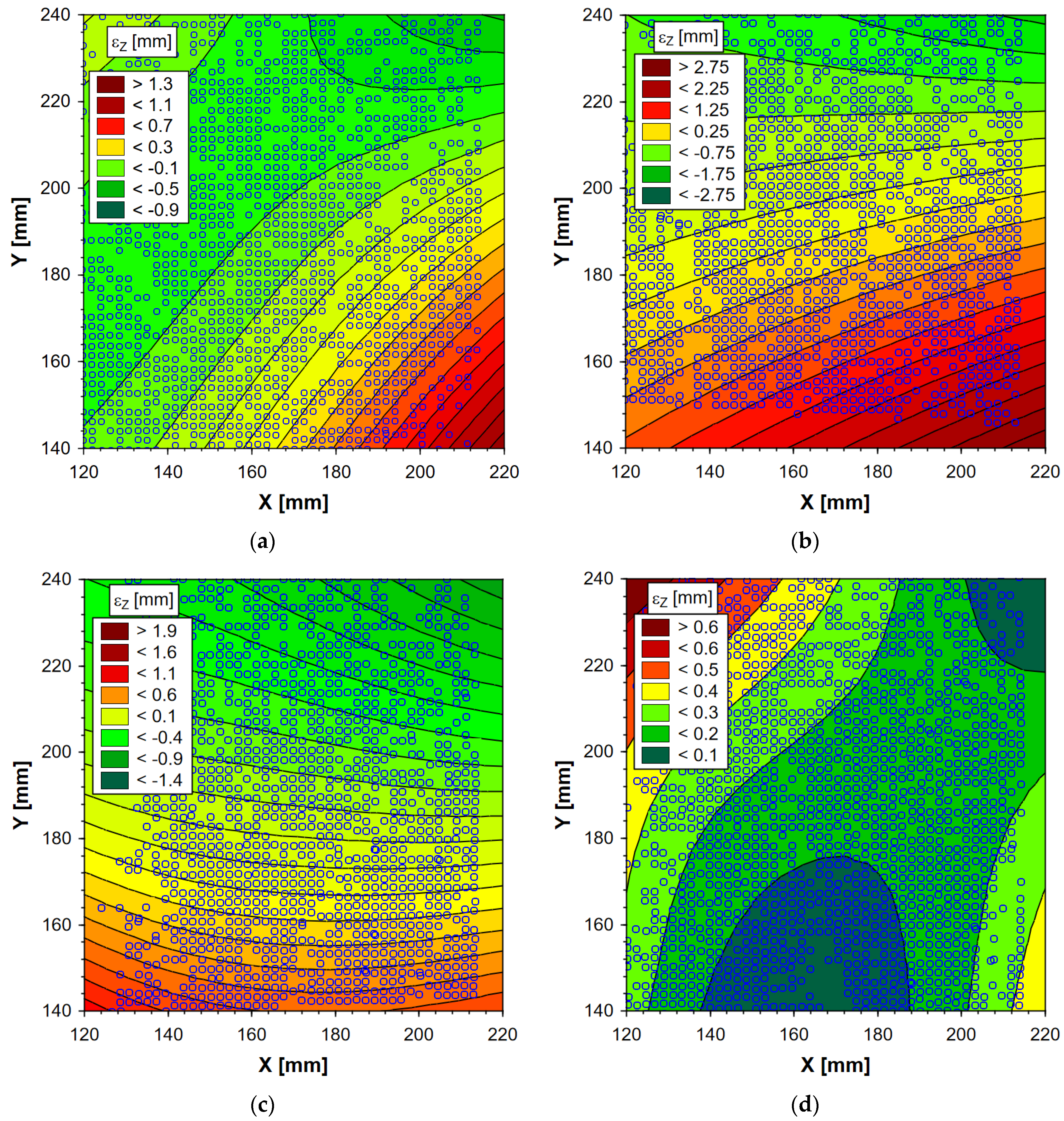
For the thus determined set of parameters related to the transformation of the robot tool coordinate system to the left camera position of the considered measurement system, the spatial position of all points of the laser pattern grid recorded in the acquired photographs was measured from four different photographic positions (different positions of the robot tool TCP point and different orientations of the associated XTYTZT coordinate system). The deviations of the measurement point coordinate value in the direction perpendicular to the projection plane (εZ), which was most meaningful in view of the metrology task in question, were analyzed. Of all three coordinates, the largest error and the largest uncertainty were noted for the measurement in this direction (Figure 14c) [42]. This involves reconstructing the depth of the measurement space from its flat representations in a forward photogrammetric indentation process. Maps of this deviation distribution (Figure 15) illustrate the distance between the laser grid points, whose position was reconstructed by measurement, and the projection plane, depending on the location of these points on this plane. The bounds of variation εZ are separated here by isolines that run differently in the individual measurement series. The largest, in absolute value, deviations are concentrated in the corners of the areas where the registered points are located, while the smallest deviations are located in the center of these areas. The measurement error of the z coordinate of the pattern points, therefore, increases from the center of the reconstructed area toward its periphery. For measurement series 1–3, the values of the z coordinate of the measurement points oscillate around zero (εZ deviation takes both positive and negative values), while in measurement series 4 the values are slightly positive. This is also confirmed by the average values of εZ deviations determined for all points registered in the measurement photographs for each measurement series (Table 6). To determine the actual shift of the reconstructed measurement points in the direction of the ZB axis, the earlier estimated correction of the standard’s position in this direction (Δz) was not applied in the measurement, but the average value of the z coordinate of the measurement points was determined for the set of results obtained for all four measurement series (totally 5800 points) (Table 6). The average value of the z coordinate was 6.14 mm, which was thus only 0.2 mm larger than the Δz correction determined in the minimization of the objective function F2 (Figure 12c). Therefore, this value can be considered as a systematic error of the developed measurement method, which can be eliminated by Δz correction. This has been regarded in the results presented in Table 6.
In the individual measuring series, the standard deviation, identified as the random error of the measured quantity, varied from 0.20 mm (measurement series 4) to 0.82 mm (measurement series 2). For the set of results covering all four measurement series together, the standard deviation was 0.51 mm. The results obtained in measurement series 2 showed the greatest scatter (Figure 15b), as the values of εZ deviation ranged from −2.06 to +2.25 mm (Table 6). The best results were achieved for measurement series 1 and 4, in which the values of εZ deviation were 1.59 and 1.22 mm, respectively.
Figure 16a shows the deviation distribution of the z coordinate value of measurement points for measurement series 4 against the theoretical probability density curve for a normal distribution. As revealed by the tests, the analyzed deviation has a normal distribution. The statistic for the Kolmogorov–Smirnov test used in this study lies outside the critical area. Thus, there are no grounds to reject the null hypothesis of normality of the tested distribution, because the test p-value is greater than the adopted significance level (α = 0.05) (Figure 16b). The points representing the relationship between the measured values and normal values of the test quantity are, in effect, arranged near a straight line, which is a graphical presentation of the normal distribution (Figure 16b). For the vast majority of points, deviations from the normality of the tested set of measurement data do not exceed ±0.2 mm (Figure 16c).
Analyzing the histogram of the εZ deviation distribution for the considered measurement series (Figure 16a), a small systematic error (0.18 mm) can be observed, which was not eliminated by the introduced Δz correction. For more than 50% of the measurement points, the deviation of the z coordinate was within ±0.2 mm, while it did not exceed ±0.3 mm in more than 70% of the cases.
4. Example of Use of the Developed Method of Measuring the Distance between the Pick Holder Base and the Cutting Head Side Surface of a Mining Machine
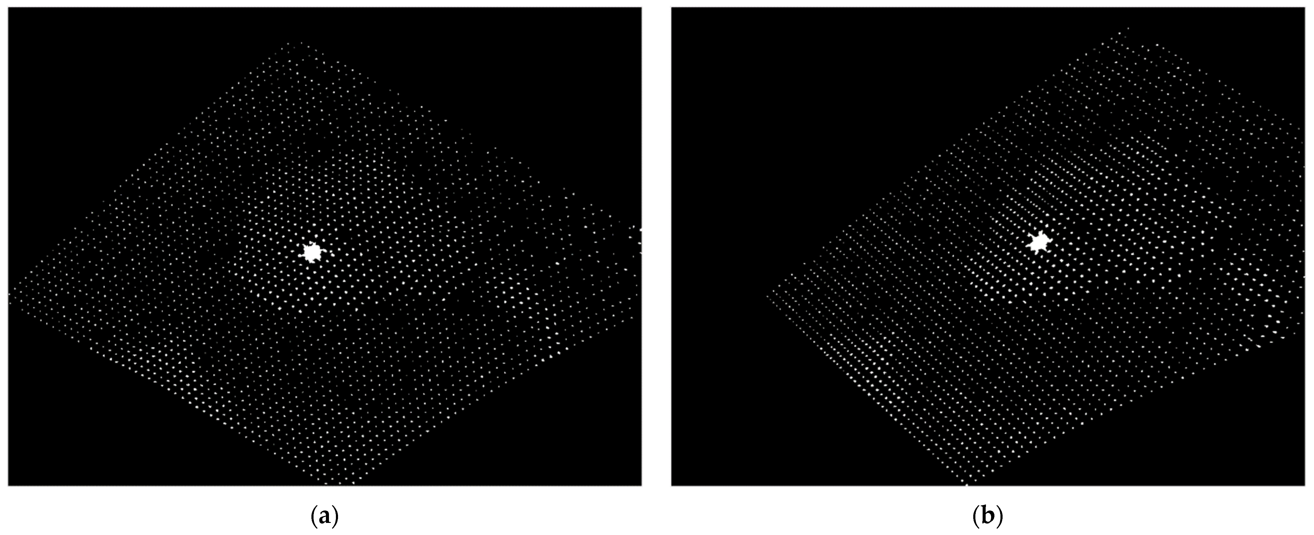
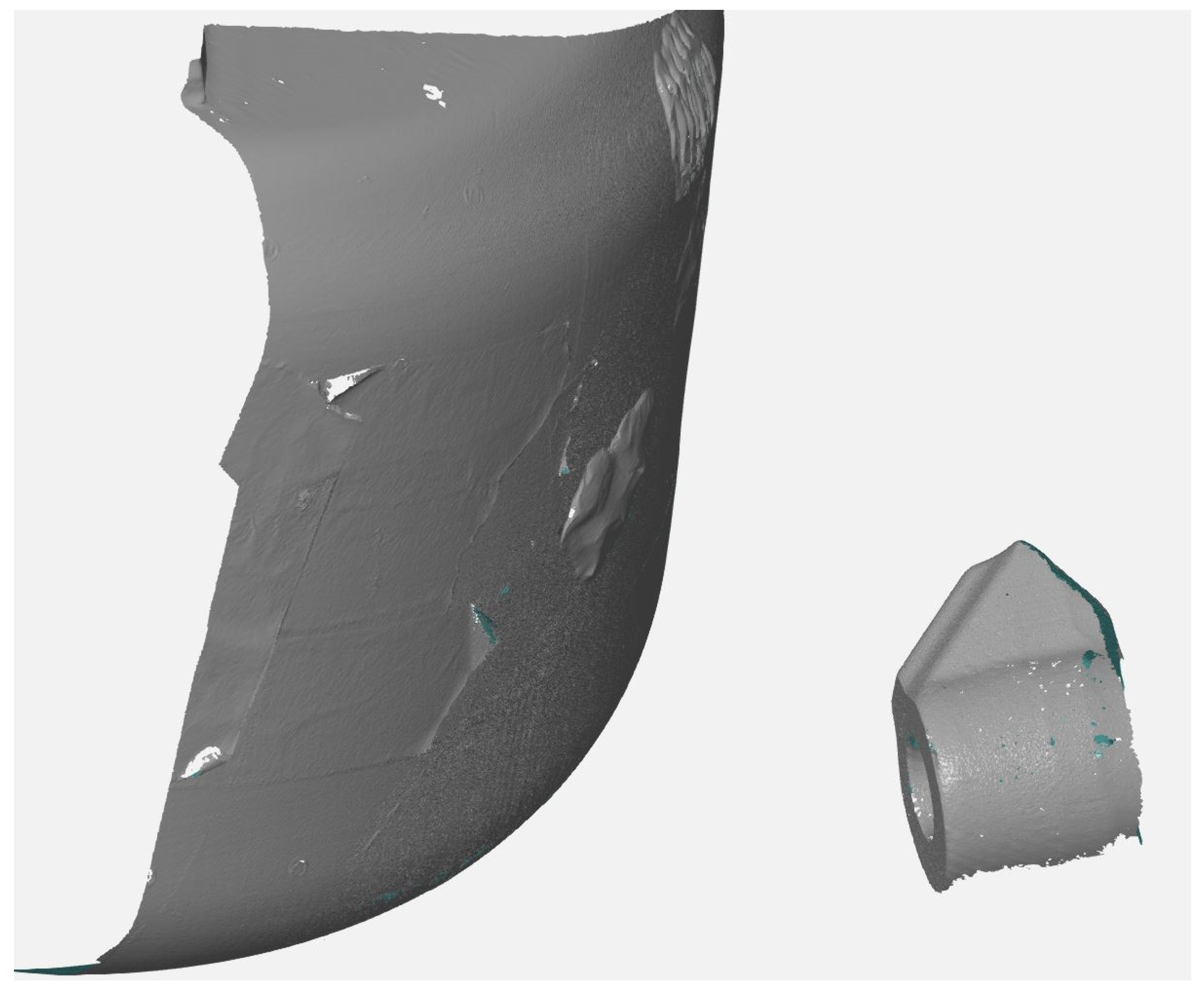
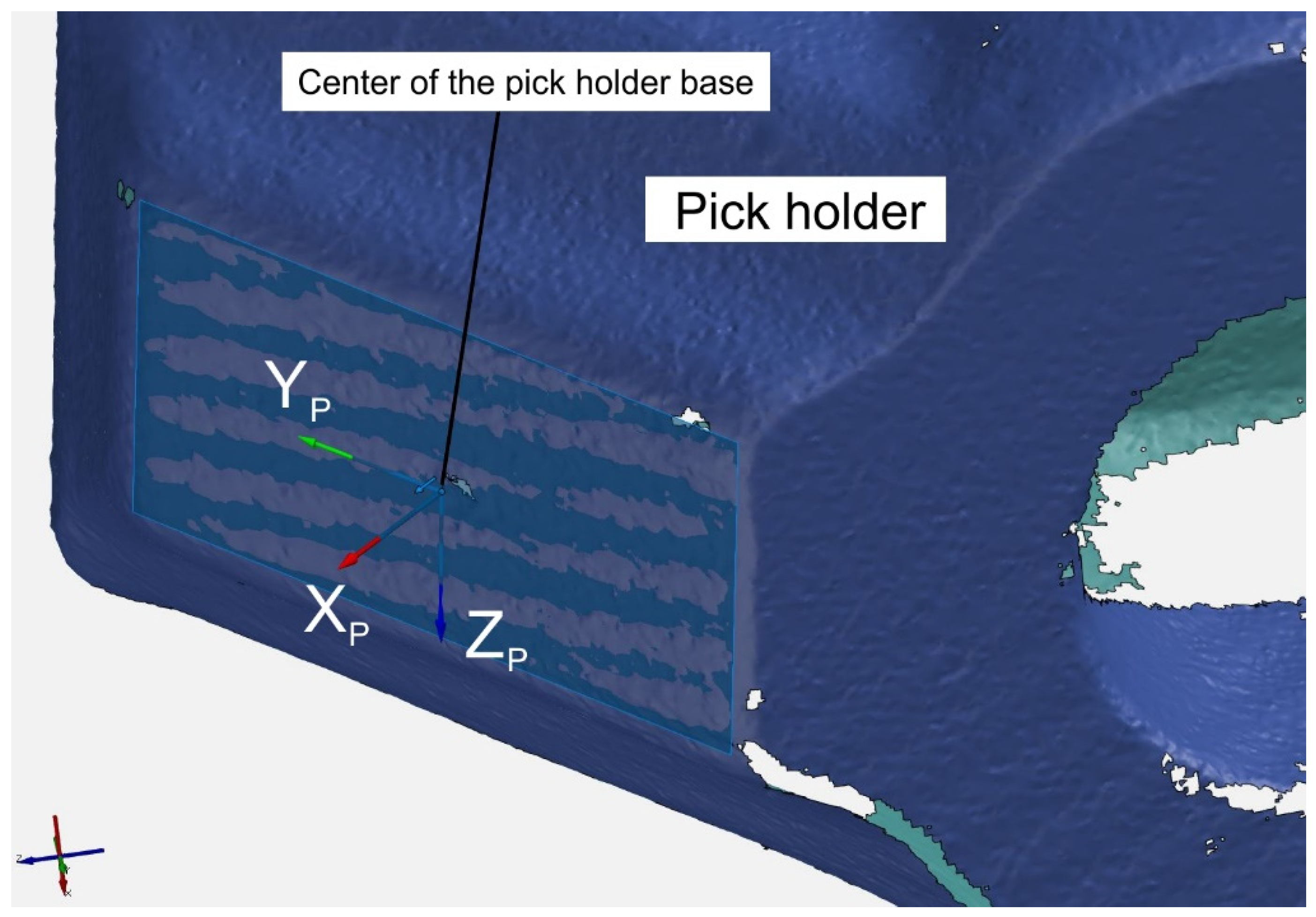
As part of the tests, the distance distribution between the pick holder base and the cutting head side surface was measured. The results of the measurements for the example pick holder position are presented in Figure 17. Input data used were the digitally processed measurement images (Figure 18) recorded by both cameras of the developed measurement system. In these images, the measurement points are identified and corresponding points are matched with each other using a specific algorithm. This results in stereo matching between the images. For confirming the metrology, the measurement results obtained with the developed method were compared with those obtained by scanning the area of interest in the cutting head side surface with the Breuckmann SmartSCAN 3D-HE structured light scanner (Figure 19). The scanner data (grids) were processed in the GOM Inspect Professional environment, which is implemented with special tools that allow construction of the various geometric elements (e.g., planes, plane figures, and solids) and comparison of grids obtained by scanning with the CAD model (Figure 20). The obtained results were used to determine the pick holder base (Figure 21). Structured light scanning has been used as the reference method due to its high precision [43]. However, a drawback of this method in terms of the measurement in question is that a large number of surface points are obtained during the scanning process. For example, an area of 100 × 100 mm extracted in the GOM Inspect software is formed by a grid of nearly 300,000 points. Moreover, irrelevant background elements are recorded during the scanning process, which must be removed in the scan processing as interference.
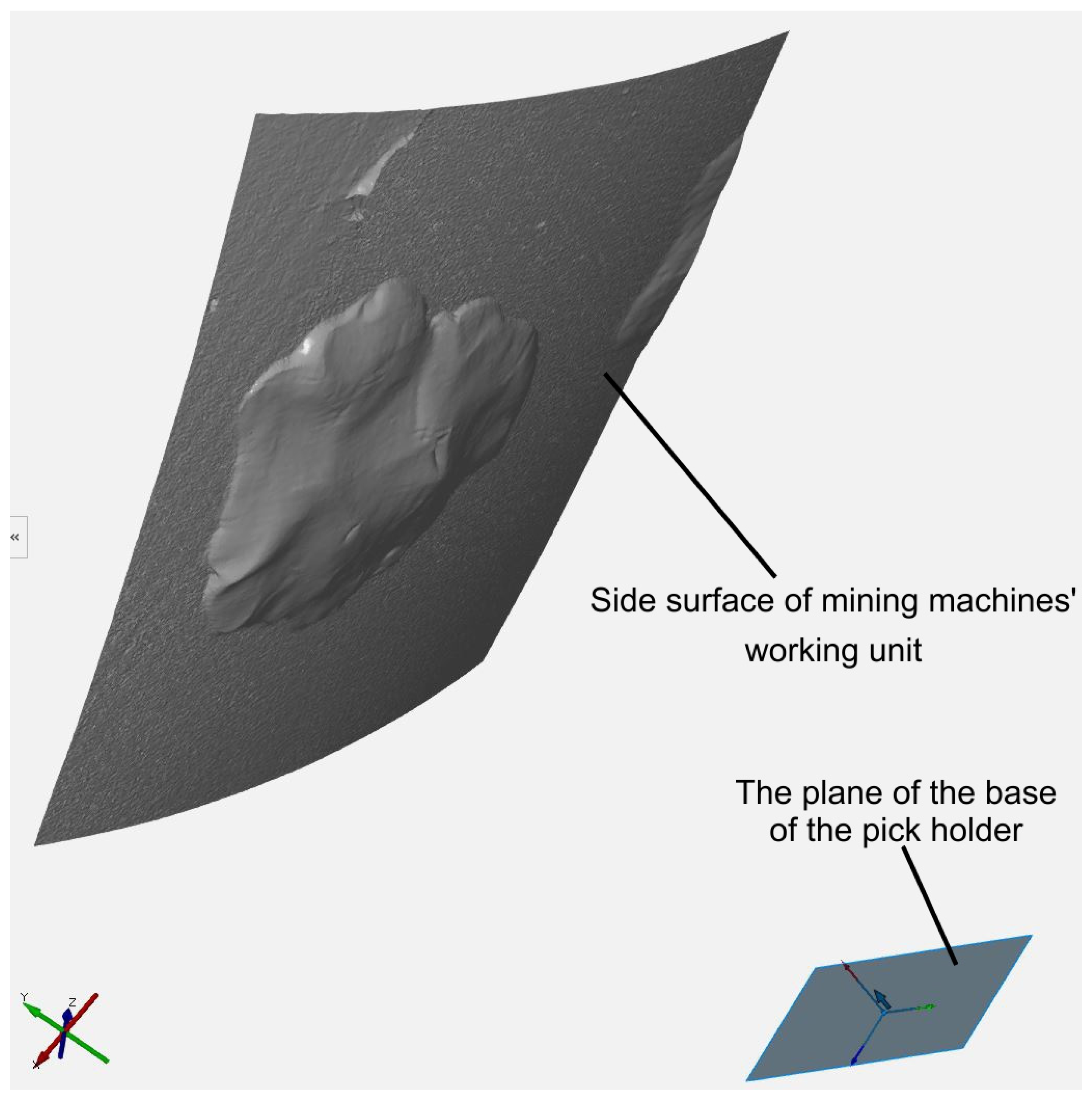
In the considered example, the pick holder base in its final position will be within the uneven part (bulge) of the cutting head side surface. During measurement, the distance distribution of this surface from the pick holder base is to be determined in points forming a grid of specified density (these points are displayed on the cutting head side surface by a laser attached to the gripper of the robot that positions the pick holders). Thus, before the pick holder reaches the set position, the robot is stopped and positioned by the software at a distance of about 100 mm from the set position (Figure 22a). Once the pick holder-positioning robot is stopped, the second robot equipped with the developed measuring system arrives at the position from which the measurement images are acquired, having previously switched on the projection device (laser displaying a grid of points on the cutting head side surface). The acquired images, which are transferred from the vision system, are then processed in the developed software on the workstation.
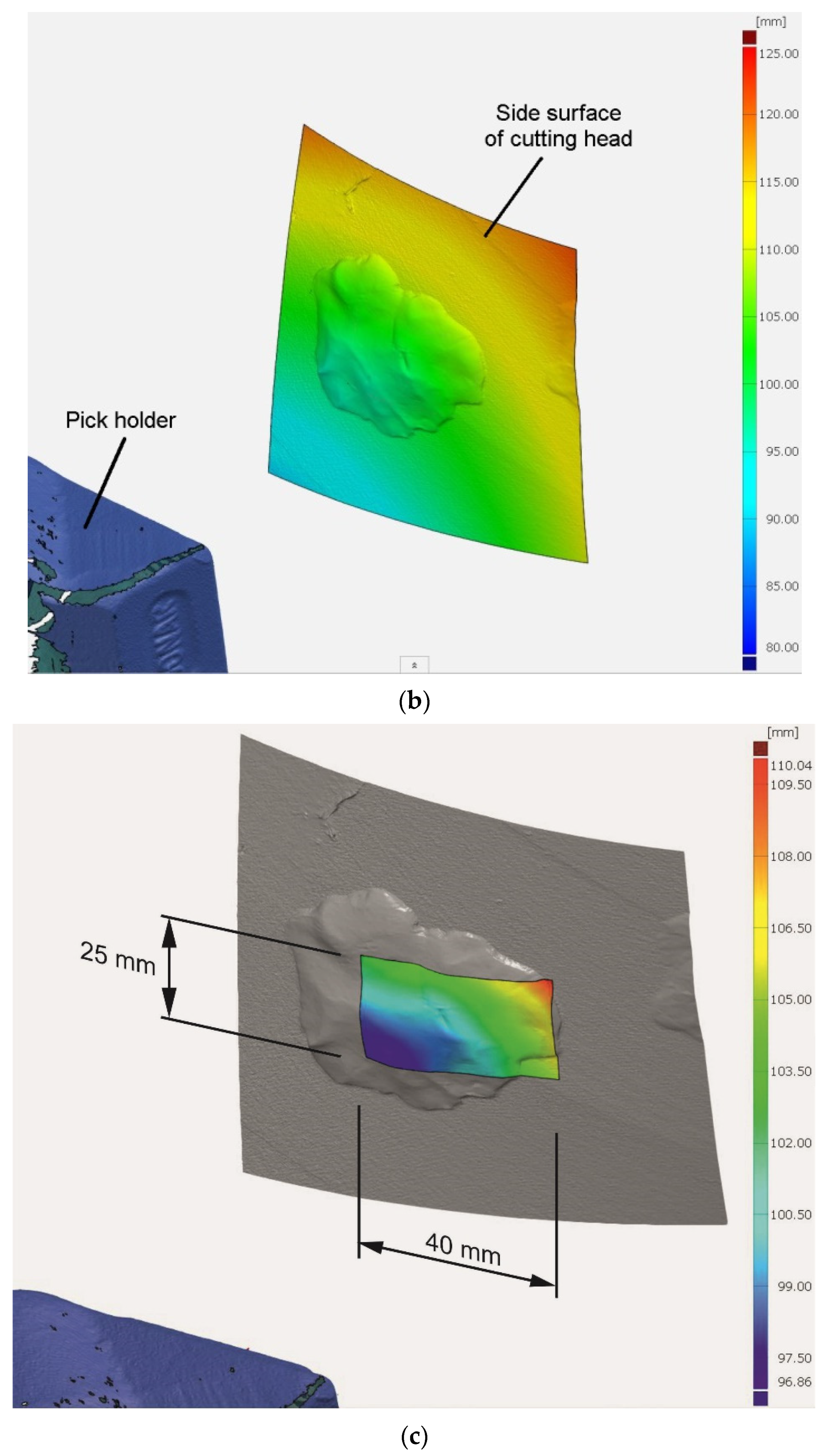
To assess the results of the measurements obtained using the developed method, the cutting head side surface was scanned using a structured light scanner. The obtained measurement results were compared using the GOM Inspect (GOM GmbH, Braunschweig, Germany) software [44,45], which was used to map the distance distribution of the cutting head side surface (a 100 × 100-mm section of the surface) from the pick holder base plane (Figure 22b). Due to the orientation of the axis of the pick holder base coordinate system, the distance between the pick holder base and cutting head side surface was measured in the direction of the XP axis in the metrology task under consideration. Due to the positioning of the pick holder on the cutting head side surface and the unevenness of the side surface, the distance between the elements was not uniform. In the studied case, the distance ranged from 89.49 to 121.78 mm, with an average value of 106.28 mm. However, in the area limited to the rectangle with dimensions corresponding to that of the pick holder base (40 × 25 mm) projected onto the cutting head side surface, the distances between the side surface and the pick holder base determined in the GOM Inspect (GOM GmbH, Braunschweig, Germany) software ranged from 96.86 to 110.04 mm (Figure 22c), with an average value of 102.15 mm.
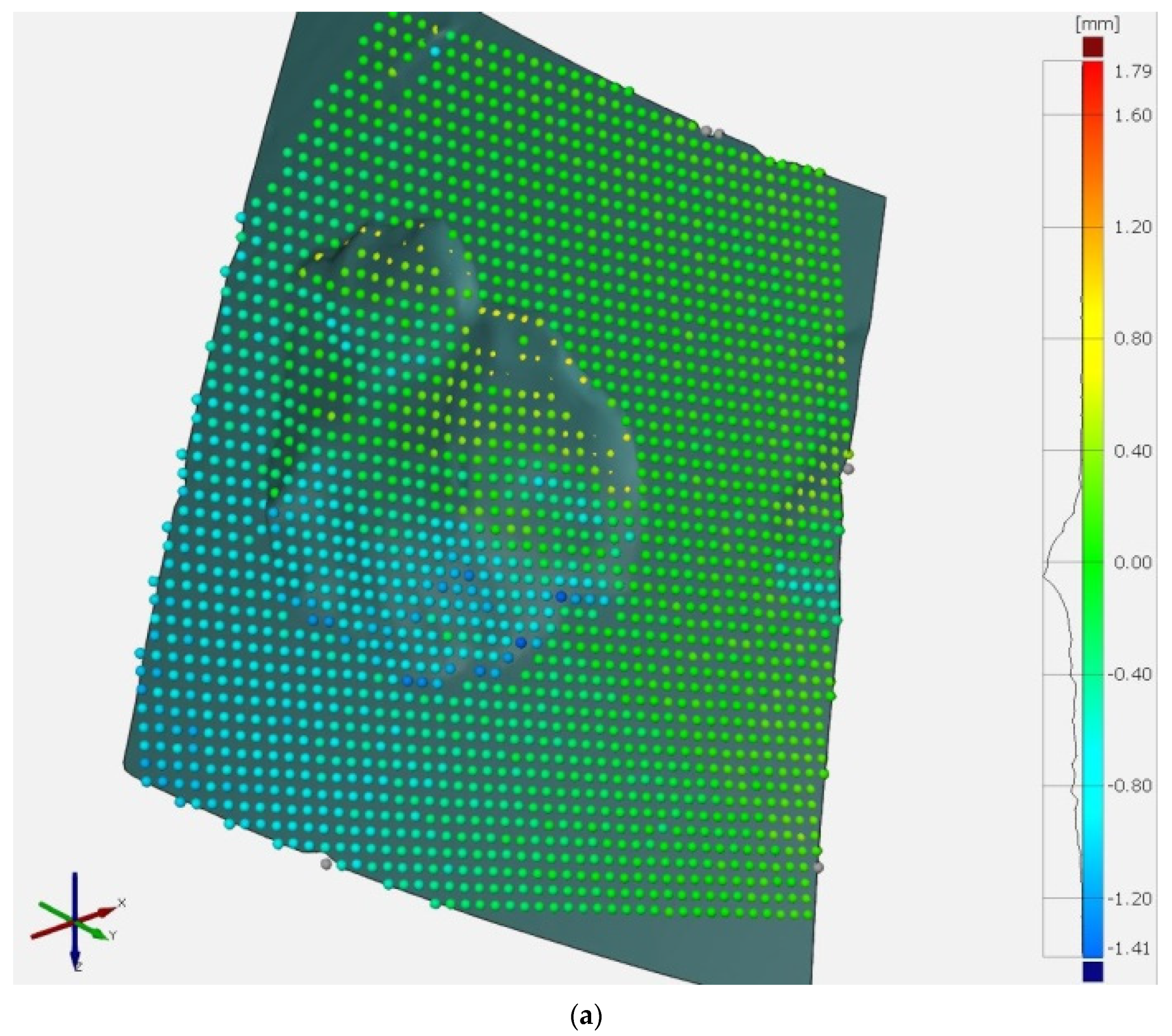
Of the 2601 measurement points of the grid displayed by the laser projection device of the developed measurement system, 2149 were identified on the images recorded by the cameras of the vision system. Stereo matching was found for these measurement points, which enabled the reconstruction of their spatial position in the XPYPZP coordinate system of the pick holder base. These points are superimposed on the surface model of the cutting head obtained by scanning with structured lighting (reference method). In the GOM Inspect (GOM GmbH, Braunschweig, Germany) environment, the coordinate deviations of the measurement points measured in the direction of the XP (εX) axis were determined, which represented the distances of these points from the cutting head side surface (Figure 23). The magnitudes of these deviations are color-coded.
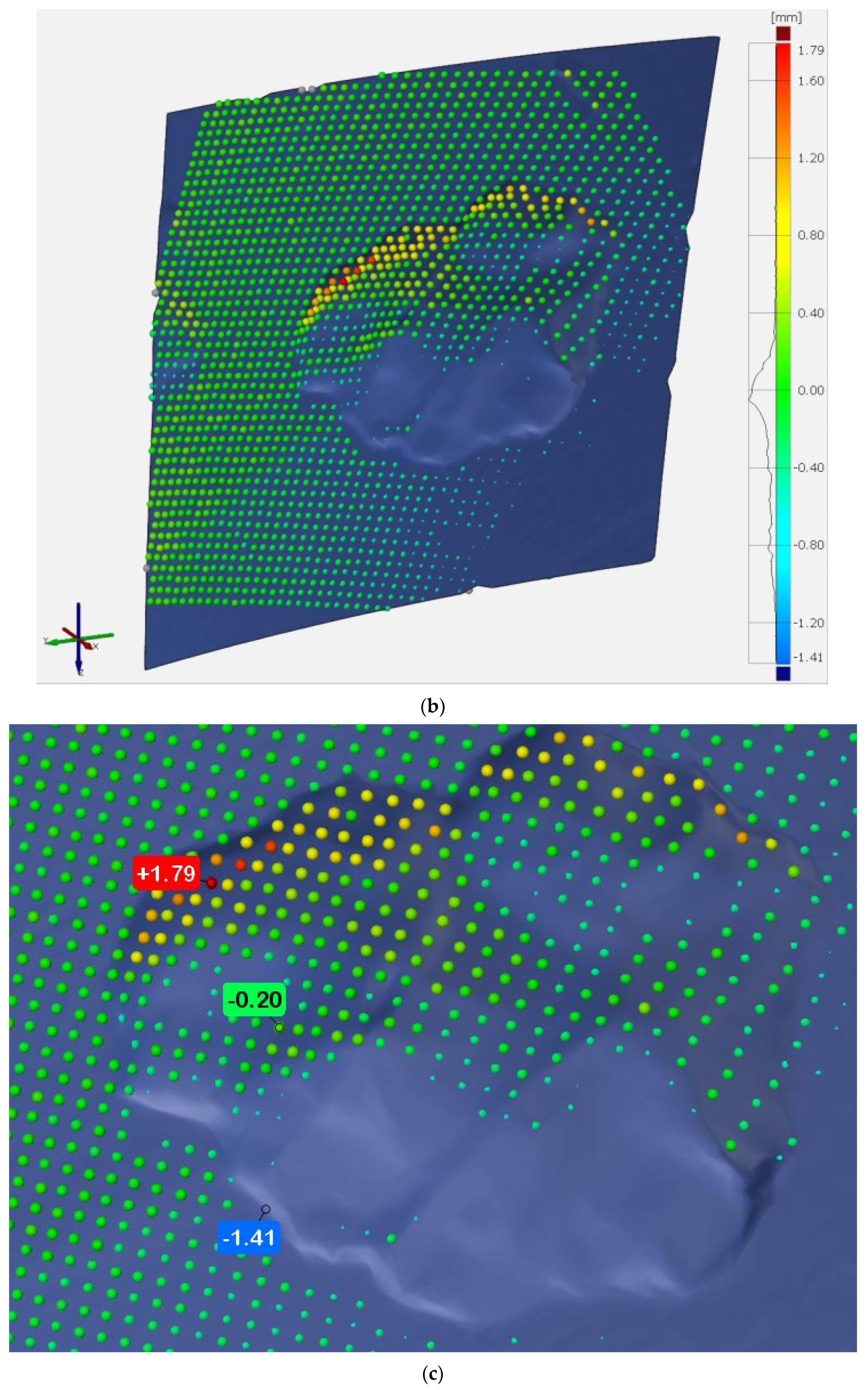
As can be seen from Figure 23, the distances of the measurement points from the cutting head side surface reconstructed using the reference method (deviation εX) assumed both positive and negative values. This implies that some of the measurement points were far from the cutting head side surface (negative deviations) (Figure 23a), while some overlapped with the side surface (positive deviations) (Figure 23b). Despite some variations, the arrangement of the points obtained from the measurement using the developed method sufficiently represented the shape of the cutting head side surface at the location for which the measurement was made. This is especially true in the area where this side had an uneven surface (bulge). The largest x-coordinate deviations were recorded for the measurement points distributed along the edge of this bulge (Figure 23c). These points or positive deviations are denoted in red and orange, and negative deviations (not visible from this side) are denoted in blue.
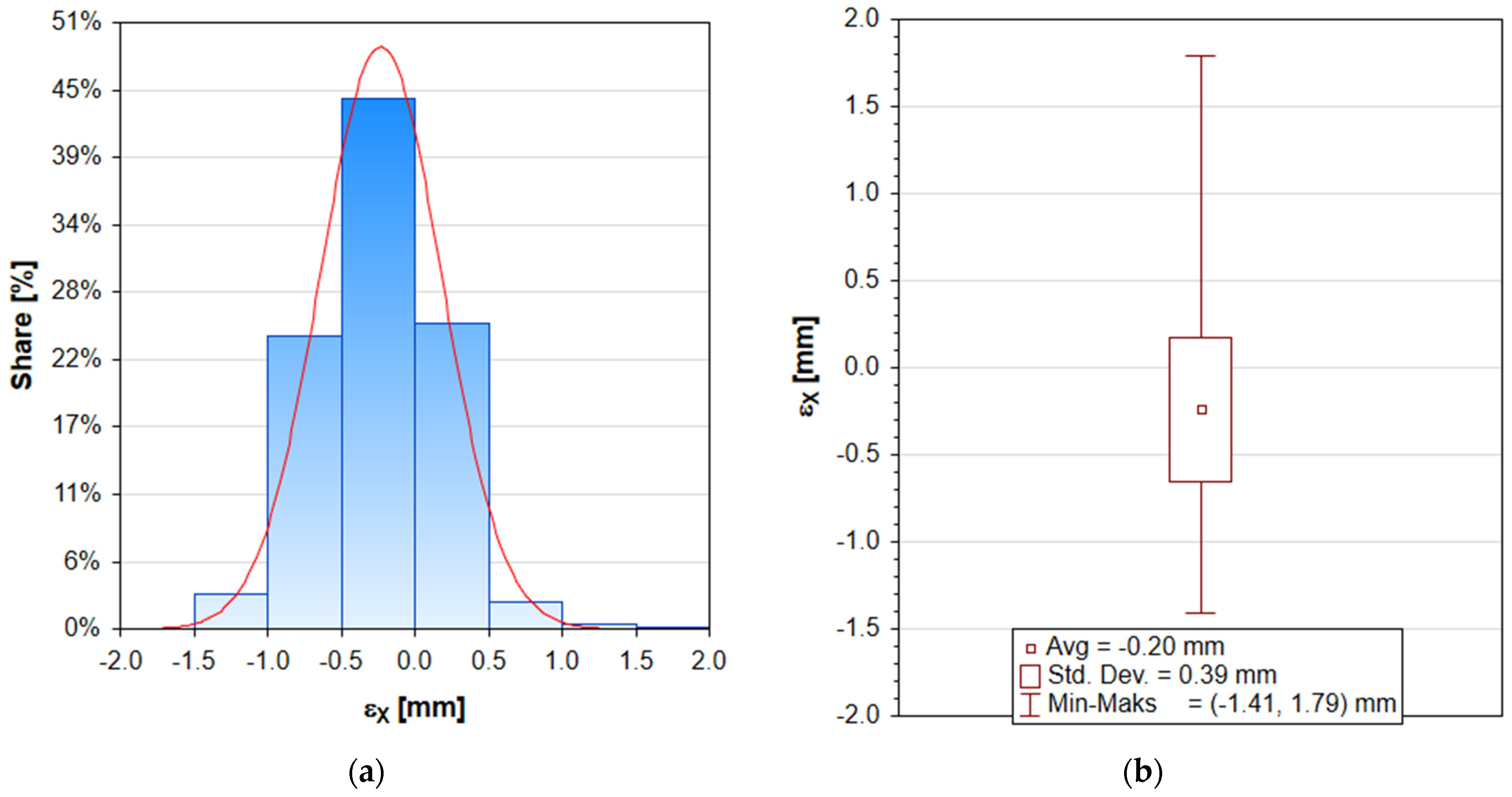
The largest share of x-coordinate deviations of the measurement points ranged between −0.5 and 0 mm (Figure 24a). These deviations were recorded for nearly 45% of the measurement points. For 70% of the measurement points, the value of εX deviation was within ±0.5 mm, while for almost 98%, the distance between the measurement points and the cutting head side surface was within ±1 mm.
The average value of the distance of the measurement points from the cutting head side surface obtained during reconstruction based on the reference method was −0.20 mm (Figure 24b), while the standard deviation, which indicates the spread of the values of the tested distances, was 0.39 mm. The largest positive deviation of the measurement points from the cutting head side surface was +1.79 mm, whereas the largest negative distance was −1.41 mm. The positions of the measurement points furthest from the cutting head side surface and the point whose distance was equal to the determined average value are shown in Figure 23c.
5. Summary and Conclusions
Monitoring of the production process is an important part of robotic manufacturing technologies. One of the main issues of production monitoring is quality control, which involves assessing the compliance of products with the technical documentation (design) at various stages of manufacturing. This problem is particularly true in the case of products synthesized from multiple components, which are joined together through various techniques such as welding and gluing, when the final effect is determined by, for instance, the mutual positioning of the components during assembly. This is also the case with the working faces of mining, tunneling, and road construction machines. The working units consist of a steel sidewall to which several pick holders are welded for fitting the cutting picks later. This side surface is usually shaped like a rotating body—a cylinder-truncated cone or paraboloid. Due to the complications associated with the positioning of the pick holders on this side surface and the fact that recovered side surfaces are often used for producing such working units, it may be necessary to adjust (directly during assembly) the positioning of the pick holders to ensure that they are welded in place. Thus, robotic technology requires:
- -
- adaptive motion control of the pick-positioning robot and the welding robot, to enable the adjustments to be made to the individual pick holders,
- -
- on-line measurement of the distance distribution between the pick holder base and the working unit of the excavating machine at the location of their attachment, to adjust the pick holders and evaluate the possibility of making a welded joint with the assumed parameters.
This article addresses the latter issue, for which a measurement system was developed, integrated with the control system of two industrial robots—one positioning the pick holders and the other positioning the measuring device during measurement. The system works based on contactless, optical measurement technology. The measuring device consists of two cameras with a convergent configuration and a laser projection device that displays a grid of points on the side surface of the working unit during measurement. In the developed system, the laser projection device was attached to the gripper of the pick holder-positioning robot.
The research aimed to calibrate the developed measurement system and assess its suitability for application in adaptive process control in robotic manufacturing technology of working bodies for mining machines.
Extensive bench testing and computer simulations performed in this study have allowed:
- -
- determination of the values of the internal and external parameters of the vision system using Matlab environment tools;
- -
- determination of the values of the parameters that bind the vision system with the robot arm to which the system is attached by solving the multidimensional minimization problem of the adopted objective function; and
- -
- determination of the deviations of the measurement points from the working unit side surface, which were obtained by reconstruction of its shape by structured light scanning (reference method).
The comparative tests revealed that the developed measurement method allows for good representation of the shape of the mining machine’s working unit side surface at the point where the respective pick holder is mounted. The method enables the determination of the distance distribution of the pick holder base from the cutting head side surface during its assembly (welding). The results showed that the value of the average distance of the measurement points from the surface they reproduce is close to zero and the value of standard deviation does not exceed 0.4 mm. For nearly three-quarters of the measurement points, this deviation is within ±0.5 mm, which indicates a good match between the measurement points and the reconstructed surface. The accuracy is sufficient for the considered application of the developed measurement method [42]. An advantage of the measurement method is its high speed of operation, resulting particularly from the lack of redundancy of measurement data, as in the case of, for example, scanning techniques. Lack of data redundancy is a prerequisite for real-time measurements when subsequent pick holders are assembled in the robotized manufacturing process to produce efficient and energy-saving mining machine working bodies.
Author Contributions
Writing—original draft preparation, P.C. and A.J.-Z.; methodology, P.C. and A.J.-Z.; investigation, A.J.-Z.; conceptualization P.C. and A.J.-Z.; supervision, P.C. All authors have read and agreed to the published version of the manuscript.
Funding
This research was funded by Silesian University of Technology, grant number 06/020/BKM21/0054.
Institutional Review Board Statement
Not applicable.
Informed Consent Statement
Not applicable.
Data Availability Statement
Not applicable.
Conflicts of Interest
The authors declare no conflict of interest.
References
- Vogt, D. A review of rock cutting for underground mining: Past, present, and future. J. S. Afr. Inst. Min. Metall. 2016, 116, 1011–1026. [Google Scholar] [CrossRef] [Green Version]
- Dewangan, S.; Chattopadhyaya, S.; Hloch, S. Wear assessment of conical pick used in coal cutting operation. Rock Mech. Rock Eng. 2014, 48, 2129–2139. [Google Scholar] [CrossRef]
- Tian, J.; Lansheng, Z.; Haifeng, Y.; Miao, W. Analysis of Stress, Strain, and Fatigue Strength of the Rotary Table of Boom-Type Roadheaders. Research Square. 2020, p. 43. Available online: https://www.researchsquare.com/article/rs-45967/v1 (accessed on 14 December 2021).
- Zhang, M. Analysis of dynamic characteristics of rotary mechanism for boom type roadheader. Appl. Mech. Mater. 2010, 37–38, 122–126. [Google Scholar] [CrossRef]
- Ebrahimabadi, A.; Goshtasbi, K.; Shahriar, K.; Cheraghi Seifabad, M. Predictive models for roadheaders’ cutting performance in coal measure rocks. Yerbilimleri/Earth Sci. 2011, 32, 89–104. [Google Scholar]
- Bołoz, Ł.; Castañeda, L.F. Computer-aided support for the rapid creation of parametric models of milling units for longwall shearers. Manag. Syst. Prod. Eng. 2018, 26, 193–199. [Google Scholar] [CrossRef] [Green Version]
- Qiang, Z.; Jun, M. Multi-objective optimization reliability design for cutting head of roadheader base on incomplete probability information. In Proceedings of the Second International Conference on Information and Computing Science, Manchester, UK, 21–22 May 2009; pp. 42–44. [Google Scholar]
- Hekimoglu, O.Z. Investigations into tilt angles and order of cutting sequences for cutting head design of roadheaders. Tunn. Undergr. Space Technol. 2018, 76, 160–171. [Google Scholar] [CrossRef]
- Jakubiec, W.; Malinowski, J. Metrologia Wielkości Geometrycznych; Wydawnictwa Naukowo-Techniczne: Warszawa, Poland, 2004. [Google Scholar]
- Tokarczyk, R. Fotogrametria cyfrowa w zastosowaniach medycznych do pomiaru ciała ludzkiego—Przegląd i tendencje rozwojowe systemów pomiarowych. Geod. Kartogr. Aerofotoznimannia 2005, 66, 233–241. [Google Scholar]
- Clarke-Hackston, N.; Belz, J.; Henneker, A. Guidance for partial face Excavation Machines. In Proceedings of the 1st International Conference on Mining Control and Guidance, Zurich, Switzerland, 24–26 June 2008; pp. 31–38. [Google Scholar]
- Sansoni, G.; Trebeschi, M.; Docchio, F. State-of-the-art and applications of 3D imaging sensors in industry, cultural heritage, medicine, and criminal investigation. Sensors 2009, 9, 568–601. [Google Scholar] [CrossRef]
- Herakovic, N. Robot Vision in Industrial Assembly and Quality Control Processes; INTECH Open Access Publisher: London, UK, 2010. [Google Scholar]
- Zivingy, M. Object distance measurement by stereo vision. Int. J. Sci. Appl. Inf. Technol. IJSAIT 2013, 2, 5–8. [Google Scholar]
- Kumanan, S. Robotics in online inspection and quality control. In Proceedings of the International Conference on Resource Utilization and Intelligent Systems, Perundurai, India, 4–6 January 2006; pp. 307–314. [Google Scholar]
- Li, X. A study on the influence of pick geometry on rock cutting based on full-scale cutting test and simulation. Adv. Mech. Eng. 2020, 12, 1687814020974499. [Google Scholar] [CrossRef]
- Cheluszka, P. Computer-aided manufacturing of working units for high-performance mining machines. Comput.-Aided Technol.-Appl. Eng. Med. 2016, 19–40. [Google Scholar]
- Cheluszka, P.; Jagieła-Zając, A. Computer support for designing cutting heads for boom-type roadheaders. In Proceedings of the Scientific Conference Abstracts, Topical Issues of Rational Use of Natural Resources, Saint Petersburg, Russia, 17–19 June 2020; Volume 2, pp. 157–159. [Google Scholar]
- Soille, P. Morphological Image Analysis: Principles and Application, 2nd ed.; Springer: Berlin/Heidelberg, Germany, 1992. [Google Scholar]
- Schmidt, J.; Niemann, H.; Vogt, S. Dense disparity maps in real-time with an application to augmented reality. In Proceedings of the Sixth IEEE Workshop on Applications of Computer Vision, Orlando, FL, USA, 3–4 December 2002; pp. 225–230. [Google Scholar]
- Deepambika, V.A.; Arunlal, S.L. Feature-based Stereo Correspondence Algorithm for the Robotic Arm Applications. Int. J. Curr. Eng. Technol. 2013, 3, 2163–2166. [Google Scholar]
- Jagieła-Zając, A.; Cheluszka, P. Measurement of the pick holders position on the side surface of the cutting head of a mining machine with the use of stereoscopic vision. IOP Conf. Ser. Mater. Sci. Eng. 2019, 679, 012005. [Google Scholar] [CrossRef]
- Cheluszka, P.; Jagieła-Zając, A. The use of a stereovision system in shape detection of the side surface of the body of the mining machine working unit. New Trends Prod. Eng. 2020, 3, 251–271. [Google Scholar] [CrossRef]
- Meng, L.; Zou, J.; Liu, G. Research on the design and automatic recognition algorithm of subsidence marks for close-range photogrammetry. Sensors 2020, 20, 544. [Google Scholar] [CrossRef] [Green Version]
- Sanfilippo, F.; Hatledal, L.I.; Zhang, H.; Fago, M.; Pettersen, K.Y. Controlling kuka industrial robots: Flexible communication interface JOpenShowVar. IEEE Robot. Autom. Mag. 2015, 20, 96–109. [Google Scholar] [CrossRef] [Green Version]
- Sangeetha, G.R.; Kumar, N.; Hari, P.R.; Sasikumar, S. Implementation of a stereo vision based system for visual feedback control of robotic arm for space manipulations. Procedia Comput. Sci. 2018, 133, 1066–1073. [Google Scholar]
- Martel, J.N.P.; Müller, J.; Conradt, J.; Sandamirskaya, Y. An active approach to solving the stereo matching problem using event-based sensors. In Proceedings of the 2018 IEEE International Symposium on Circuits and Systems (ISCAS), Florence, Italy, 27–30 May 2018; pp. 1–5. [Google Scholar]
- Alagoz, B.B. A note on depth estimation from stereo imaging systems. Comput. Sci. 2016, 1, 8–13. [Google Scholar]
- Wang, L.; Liu, Z.; Zhang, Z. Feature based stereo matching using two-step expansion. Math. Probl. Eng. 2014, 2014, 452803. [Google Scholar] [CrossRef] [Green Version]
- Xu, G.; Zhang, Z. Epipolar Geometry in Stereo, Motion and Object Recognition, 1st ed.; Springer: Berlin/Heidelberg, Germany, 1996. [Google Scholar]
- Gao, Z.; Hwang, A.; Zhai, G.; Peli, E. Correcting geometric distortions in stereoscopic 3D imaging. PLoS ONE 2018, 13, e0205032. [Google Scholar] [CrossRef] [PubMed]
- Dyskin, A.V.; Basarir, H.; Doherty, J.; Elchalakani, M.; Joldes, G.R.; Karrech, A.; Lehane, B.; Miller, K.; Pasternak, E.; Shufrin, I.; et al. Computational monitoring in real time: Review of methods and applications. Geomech. Geophys. Geo-Energy Geo-Resour. 2018, 4, 235–271. [Google Scholar] [CrossRef] [Green Version]
- Yuda, M.; Xiangjun, Z.; Weiming, S.; Shaofeng, L. Target accurate positioning based on the point cloud created by stereo vision. In Proceedings of the 23rd International Conference on Mechatronics and Machine Vision in Practice, Nanjing, China, 28–30 November 2016; Volume 1. [Google Scholar]
- Nedevschi, S.; Marita, T.; Vaida, M.; Danescu, R.; Frentiu, D.; Oniga, F.; Pocol, C.; Moga, D. Camera calibration method for stereo measurement. J. Control Eng. Appl. Inform. 2002, 4, 21–28. [Google Scholar]
- Belhaoua, A.; Kohler, S.; Hirsch, E. Estimation of 3D reconstruction errors in a stereo-vision system. Proc. SPIE 2009, 7390, 73900X. [Google Scholar]
- Levenberg, K. A method for the solution of certain non-linear problems in least squares. Q. Appl. Math. 1944, 2, 164–168. [Google Scholar] [CrossRef] [Green Version]
- Marquardt, D. An algorithm for least-squares estimation of nonlinear parameters. SIAM J. Appl. Math. 1963, 11, 431–441. [Google Scholar] [CrossRef]
- Wilson, P.; Mantooth, H.A. Model-Based Optimization Techniques. In Model-Based Engineering for Complex Electronic Systems; Newnes: London, UK, 2013; p. 536. [Google Scholar]
- Boroń, A.; Kudła, J.; Ondrusek, C. Application of genetic algorithm and Levenberg-Marquardt method to approximation of synchronous machine spectral inductances. Sci. Issues Sil. Univ. Technol. Electr. Ser. 1999, 168, 113–124. [Google Scholar]
- Gavin, H.P. The Levenberg-Marquardt Algorithm for Nonlinear Least Squares Curve-Fitting Problems; Department of Civil and Environmental Engineering, Duke University: Durham, NC, USA, 2020; p. 19. Available online: https://people.duke.edu/~hpgavin/ce281/lm.pdf (accessed on 31 October 2021).
- Kanzowa, C.; Yamashita, N.; Fukushima, M. Levenberg-Marquardt methods with strong local convergence properties for solving nonlinear equations with convex constraints. J. Comput. Appl. Math. 2004, 172, 375–397. [Google Scholar] [CrossRef] [Green Version]
- Cheluszka, P. Metrology of Mining Machines Working Units; Publishing House of the Silesian University of Technology: Gliwice, Poland, 2012. (In Polish) [Google Scholar]
- Mendřický, R. Determination of measurement accuracy of optical 3D scanners. MM Sci. J. 2016, 2016, 1565–1572. [Google Scholar] [CrossRef] [Green Version]
- Vladimir, A.G. Point clouds registration and generation from stereo images. Inf. Content Process. 2016, 3, 193–199. [Google Scholar]
- Bell, S. Measurement Good Practice Guide, 2nd ed.; National Physical Laboratory: Teddington, UK, 1999. [Google Scholar]
Figure 1.
Roadheader’s extending heads: (a) decommissioned, (b) in the course of removing the pick holders, and (c) after removing the pick holders.
Figure 1.
Roadheader’s extending heads: (a) decommissioned, (b) in the course of removing the pick holders, and (c) after removing the pick holders.

Figure 2.
(a) Test bench, (b) schematic diagram of the connection of measurement instrumentation components to the robot control system, (c) vision system during robot positioning of the pick holder: 1—KUKA KR 16-2 robot positioning pick holders, 2—linear unit KL 250-3, 3—positioner PEV-1-2500, 4—cutting head side surface, 5—gripper, 6—controller, 7—PoE switch, 8—vision system, 9—laser projection device, 10—KUKA KR 5 robot positioning vision system cameras, and 11—positioned pick holder.

Figure 3.
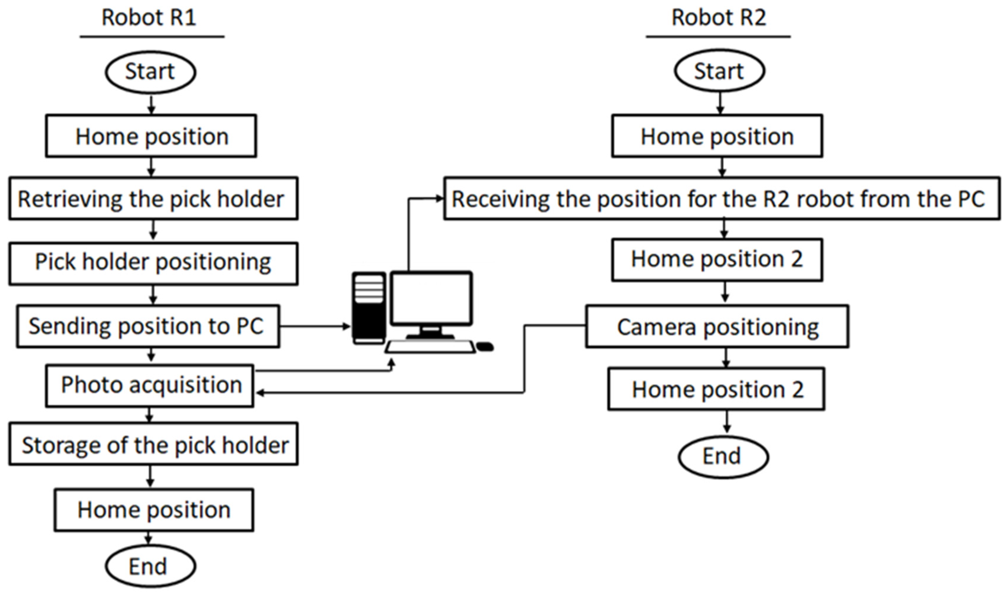
The simplified algorithm for controlling the robots during measurement.

Figure 4.
Schematic diagram of communication between the robots and the workstation.

Figure 5.
A grid of points in the coordinate system associated with: (a) the vision system’s left camera, (b) the robot tool’s pick holder base, and (c) the relationship between the coordinate system associated with the vision system and the coordinate system associated with the vision system’s left camera.

Figure 6.
Calibration plate and its position relative to the camera array during calibration: 1—left camera (initial coordinate system of the video system) and 2—right camera.
Figure 6.
Calibration plate and its position relative to the camera array during calibration: 1—left camera (initial coordinate system of the video system) and 2—right camera.

Figure 7.
Spatial position measurement model of a point on a robotic workstation using a stereo-vision system.
Figure 7.
Spatial position measurement model of a point on a robotic workstation using a stereo-vision system.

Figure 8.
Laser grid of points projected onto XBYB projection plane.

Figure 9.
Arrangement of laser grid measurement points used during calibration of the developed measurement system.
Figure 9.
Arrangement of laser grid measurement points used during calibration of the developed measurement system.

Figure 10.
Influence of the initial values of the transformation parameters on the results of minimizing the objective function F1: dependence of the mean value (a) and standard deviation (b) on selected components of the translation and rotation vectors of the left camera coordinate system; dependence of the mean value (c) and standard deviation (d) on the displacement of the central point of the pattern.

Figure 11.
Values of basic statistics describing the distributions of coordinate deviations of the points obtained from measurements for transformation parameters resulting from minimization of the considered objective function.
Figure 11.
Values of basic statistics describing the distributions of coordinate deviations of the points obtained from measurements for transformation parameters resulting from minimization of the considered objective function.

Figure 12.
Values of the sought parameters derived from the minimization of the objective functions under consideration: (a) components of the translation vector of the coordinate system XTYTZT to the point KL, (b) angles of rotation of the coordinate system XTYTZT, and (c) shift of the laser grid central point (pattern) in the coordinate system XBYBZB.

Figure 13.
(a) Course of minimization of the objective function F2 and (b) the values of the sought parameters worked out in subsequent iterations.
Figure 13.
(a) Course of minimization of the objective function F2 and (b) the values of the sought parameters worked out in subsequent iterations.

Figure 14.
Comparison of the values of coordinates of nine measurement points obtained in four measurement series against nominal values of the model for parameters obtained from minimization of the objective function F2: (a) X coordinate, (b) Y coordinate, (c) Z coordinate.
Figure 14.
Comparison of the values of coordinates of nine measurement points obtained in four measurement series against nominal values of the model for parameters obtained from minimization of the objective function F2: (a) X coordinate, (b) Y coordinate, (c) Z coordinate.

Figure 15.
Distribution maps of coordinate deviations of measurement points in the direction of ZB axis of the robot base coordinate system: (a) measurement series 1, (b) measurement series 2, (c) measurement series 3, and (d) measurement series 4.
Figure 15.
Distribution maps of coordinate deviations of measurement points in the direction of ZB axis of the robot base coordinate system: (a) measurement series 1, (b) measurement series 2, (c) measurement series 3, and (d) measurement series 4.

Figure 16.
Coordinate deviation of measurement points in the direction of ZB axis for measurement series 4: (a) distribution histogram, (b) normality diagram, and (c) normality deviation diagram.
Figure 16.
Coordinate deviation of measurement points in the direction of ZB axis for measurement series 4: (a) distribution histogram, (b) normality diagram, and (c) normality deviation diagram.

Figure 17.
(a) Example for setting the pick holder (b) with projected laser grid of points.

Figure 18.
Images resulting from the processing of measurement photographs: (a) left camera image and (b) right camera image.
Figure 18.
Images resulting from the processing of measurement photographs: (a) left camera image and (b) right camera image.

Figure 19.
Scanning grids of the cutting head side surface and pick holder, imported into GOM Inspect Professional (GOM GmbH, Braunschweig, Germany).
Figure 19.
Scanning grids of the cutting head side surface and pick holder, imported into GOM Inspect Professional (GOM GmbH, Braunschweig, Germany).

Figure 20.
Design of the pick holder base plane and the XPYPZP coordinate system hooked in the middle of the pick holder base built-in GOM Inspect Professional (GOM GmbH, Braunschweig, Germany).
Figure 20.
Design of the pick holder base plane and the XPYPZP coordinate system hooked in the middle of the pick holder base built-in GOM Inspect Professional (GOM GmbH, Braunschweig, Germany).

Figure 21.
Spatial orientation of the pick holder base plane relative to the cutting head side surface.
Figure 21.
Spatial orientation of the pick holder base plane relative to the cutting head side surface.

Figure 22.
(a) Position of the pick holder relative to the cutting head side surface during measurement, (b) distribution map of distances of the cutting head side surface from the pick holder base plane obtained using GOM Inspect (GOM GmbH, Braunschweig, Germany) software, and (c) distribution map of these distances in the area limited to the dimensions of the pick holder base.


Figure 23.
Distribution maps of the distances of measurement points from the cutting head side surface obtained by structural light scanning (reference method): (a) view of measurement points from the outer side of the cutting head side surface, (b) view of measurement points from the inner side of the cutting head side surface, and (c) zoomed-in view of the area of the largest deviation (inner side of cutting head side).


Figure 24.
(a) Histogram of the distribution of coordinate deviations of the measuring points from the cutting head side surface measured in the direction of the XP axis of the coordinate system associated with the pick holder base and (b) basic statistics of this distribution.
Figure 24.
(a) Histogram of the distribution of coordinate deviations of the measuring points from the cutting head side surface measured in the direction of the XP axis of the coordinate system associated with the pick holder base and (b) basic statistics of this distribution.


Table 1.
KUKA MXG20 camera and Tamron M118FM25 lens specifications.
| Camera Parameters | ||
|---|---|---|
| Type of Sensor | 1/1.8″ Progressive Scan CCD | |
| Resolution | 1624 × 1228 px | |
| Frame rate max | 27 fps | |
| Pixel Formats | Mono 8, Mono 12, Mono 12 Packed | |
| Lens Parameters | ||
| Focal length | 25 mm | |
| Aperture range | 1.6–16 | |
| Angel of view (horizontal × vertical) | 1/1.8 | 16.6° × 12.5° |
| 1/2 | 14.6° × 11.0° | |
| 1/3 | 11.0° × 8.2° | |
| Back focus (in air) | 12.92 | |
Table 2.
Internal camera parameters obtained during calibration in the Matlab environment.
| Left Camera | Right Camera | |
|---|---|---|
| Image size | ||
| Radial distortion | ||
| Tangential distortion | ||
| Focal length | ||
| Principal point | ||
| Intrinsic matrix | ||
| Mean reprojection error | 0.4987 | 0.4650 |
Table 3.
External parameters of the vision system obtained during calibration in the Matlab environment.
Table 3.
External parameters of the vision system obtained during calibration in the Matlab environment.
| Rotation of camera 2 | |
| Translation of camera 2 | |
| Fundamental matrix | |
| Essential matrix | |
| Mean reprojection error | 0.4818 |
Table 4.
Combinations of endpoints of the sections for which the slope angles αHV are determined.
| i | 1 | 2 | 3 | 4 | 5 | 6 | 7 | 8 | 9 | |
|---|---|---|---|---|---|---|---|---|---|---|
| j | ||||||||||
| 1 | x | + | + | + | + | + | + | + | + | |
| 2 | + | x | + | + | ||||||
| 3 | + | + | x | + | + | + | ||||
| 4 | + | + | x | + | ||||||
| 5 | + | + | + | x | + | + | ||||
| 6 | + | + | + | x | + | + | ||||
| 7 | + | + | + | x | + | |||||
| 8 | + | + | + | + | x | + | ||||
| 9 | + | + | x | |||||||
Table 5.
Search area for the starting point for the minimization process of the studied objective functions.
Table 5.
Search area for the starting point for the minimization process of the studied objective functions.
| Parameter | Range | Parameter | Range | Parameter | Range |
|---|---|---|---|---|---|
| K1.X [mm] | 〈−120, −100〉 | K1.A [deg] | 0 | Δx [mm] | 〈−10, 10〉 |
| K1.Y [mm] | 0 | K1.B [deg] | 〈0, 15〉 | Δy [mm] | 〈−10, 10〉 |
| K1.Z [mm] | 0 | K1.C [deg] | 0 | Δz [mm] | 0 |
Table 6.
Summary of the basic statistics of deviations in the direction of ZB axis of all measurement points registered in individual measurement series.
Table 6.
Summary of the basic statistics of deviations in the direction of ZB axis of all measurement points registered in individual measurement series.
| Measurement Series No. | Number of Measurement Points | εZ [mm] | |||
|---|---|---|---|---|---|
| Min | Max | Avg | Std. Dev. | ||
| 1 | 1508 | −0.75 | 0.84 | −0.09 | 0.28 |
| 2 | 1417 | −2.06 | 2.25 | −0.07 | 0.82 |
| 3 | 1298 | −1.13 | 1.69 | −0.05 | 0.49 |
| 4 | 1601 | −0.43 | 0.79 | 0.18 | 0.20 |
| Overall | 5824 | −2.06 | 2.25 | 0.00 | 0.51 |
Publisher’s Note: MDPI stays neutral with regard to jurisdictional claims in published maps and institutional affiliations. |
© 2022 by the authors. Licensee MDPI, Basel, Switzerland. This article is an open access article distributed under the terms and conditions of the Creative Commons Attribution (CC BY) license (https://creativecommons.org/licenses/by/4.0/).
Share and Cite
MDPI and ACS Style
Cheluszka, P.; Jagieła-Zając, A. Validation of a Method for Measuring the Position of Pick Holders on a Robotically Assisted Mining Machine’s Working Unit. Energies 2022, 15, 295. https://doi.org/10.3390/en15010295
AMA Style
Cheluszka P, Jagieła-Zając A. Validation of a Method for Measuring the Position of Pick Holders on a Robotically Assisted Mining Machine’s Working Unit. Energies. 2022; 15(1):295. https://doi.org/10.3390/en15010295
Chicago/Turabian StyleCheluszka, Piotr, and Amadeus Jagieła-Zając. 2022. "Validation of a Method for Measuring the Position of Pick Holders on a Robotically Assisted Mining Machine’s Working Unit" Energies 15, no. 1: 295. https://doi.org/10.3390/en15010295
Note that from the first issue of 2016, this journal uses article numbers instead of page numbers. See further details here.