
Integration of Classical Mathematical Modeling with an Artificial Neural Network for the Problems with Limited Dataset


AGH University of Science and Technology, 30 Mickiewicza Ave., 30059 Cracow, Poland
*
Author to whom correspondence should be addressed.
Energies 2021, 14(16), 5127; https://doi.org/10.3390/en14165127
Submission received: 24 June 2021
/
Revised: 12 August 2021
/
Accepted: 17 August 2021
/
Published: 19 August 2021
(This article belongs to the Special Issue Development of Advanced Models for Analysis and Simulation of Fuel Cells)
Abstract
:One of the most common problems in science is to investigate a function describing a system. When the estimate is made based on a classical mathematical model (white-box), the function is obtained throughout solving a differential equation. Alternatively, the prediction can be made by an artificial neural network (black-box) based on trends found in past data. Both approaches have their advantages and disadvantages. Mathematical models were seen as more trustworthy as their prediction is based on the laws of physics expressed in the form of mathematical equations. However, the majority of existing mathematical models include different empirical parameters, and both approaches inherit inevitable experimental errors. Simultaneously, the approximation of neural networks can reproduce the solution exceptionally well if fed sufficient data. The difference is that an artificial neural network requires big data to build its accurate approximation, whereas a typical mathematical model needs several data points to estimate an empirical constant. Therefore, the common problem that developers meet is the inaccuracy of mathematical models and artificial neural networks. Another common challenge is the mathematical models’ computational complexity or lack of data for a sufficient precision of the artificial neural networks. Here we analyze a grey-box solution in which an artificial neural network predicts just a part of the mathematical model, and its weights are adjusted based on the mathematical model’s output using the evolutionary approach to avoid overfitting. The performance of the grey-box model is statistically compared to a Dense Neural Network on benchmarking functions. With the use of Shaffer procedure, it was shown that the grey-box approach performs exceptionally well when the overall complexity of a problem is properly distributed with the mathematical model and the Artificial Neural Network. The obtained calculation results indicate that such an approach could increase precision and limit the dataset required for learning. To show the applicability of the presented approach, it was employed in modeling of the electrochemical reaction in the Solid Oxide Fuel Cell’s anode. Implementation of a grey-box model improved the prediction in comparison to the typically used methodology.
1. Introduction
Predicting the output of a system is one of the most frequent tasks in the fields of research in engineering, economics, medicine, etc. It may be a performance estimation of a device, cost analysis, or predictive medicine. Whenever possible, classical mathematical models are developed based on the laws of physics, observations, and, unavoidably, assumptions. In this paper, the phrase “the classical mathematical model” is used as an equivalent of white-box model. Mathematical models often can be inaccurate, incomplete, or very hard to formulate due to gaps in the existing knowledge. In such cases, to be able to predict a system’s output, approximation methods are used. Computational models known as Artificial Neural Networks (ANN) have brought a vast improvement to predictions in many fields. An ANN can achieve excellent performance in function approximation, comparable to accurate mathematical models [1]. For such high accuracy, an ANN needs a lot of data. Obtaining enough samples may be expensive and time-consuming, and, in effect, unprofitable. Data numerousness is mostly dependent on the complexity of the process one wants to predict. As a vivid example of such a problem, we can offer a fuel cell modeling a multiscale and interdisciplinary problem. The fuel cell models are hard to generalize over different types and have very complicated models because of various species transport phenomena and electrochemical reaction kinetics [2,3]. Obtaining the necessary tomographic data for electrodes’ microstructure characterization costs a few months of operator work [4,5]. For such a problem, collecting more than twenty data points per dimension would take years and therefore is infeasible in many cases [6,7,8].
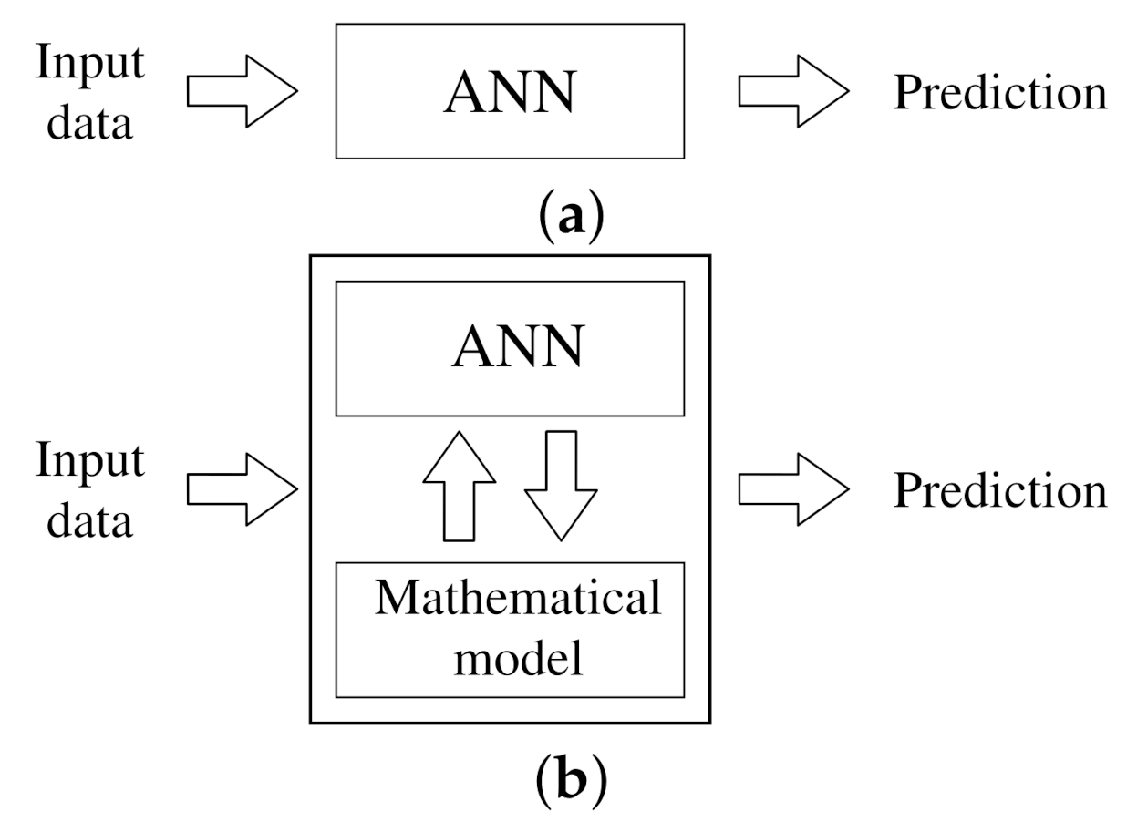
In this paper, we address the problem of data shortage by integrating the classical mathematical model with an artificial neural network as presented in Figure 1. For clarification, we will refer to our implementation of a grey box model as the Interactive Mathematical modeling-Artificial Neural Network (IMANN). The approach presented in this study stems from the fact that every mathematical model’s solution, including the example given above, is represented as a function or a set of functions. The method consists of determining the most uncertain parts of a mathematical model or lacking a theoretical description, and substituting them with a prediction of an ANN, instead of using the mathematical model or the ANN alone. With that being said, the work with the IMANN differs from the practice with a regular ANN. In a conventional procedure, a dataset is divided into training and test data. In addition to these steps, the IMANN requires to divide the problem into two parts. The mathematical model describes one of them, and the artificial neural network approximates the other. The decision regarding this division is a crucial part of working with IMANN, which affects the architecture of the network as well as the data. The underlying research of this paper is to improve the predictive accuracy under a limited dataset, which is understood as less than twenty points per input dimensionality. This research problem is addressed by incorporating an artificial neural network to predict different parts of benchmark functions, which are regarded as a general representation of mathematical models. The ANN is learned based on the mathematical model’s output. A detailed description is presented in Section 3. In practice, it might be understood that the ANN prediction replaces only some equations in a model (or even just a part of an equation) and adapts to the system’s behavior. As an example, let us consider a system of equations in which one of the equations is replaced by the prediction done by an artificial neural network. The obtained approximation values of that function would be forced by the numerical model to fulfill all equations in the system. If the prediction is incorrect there would be a discrepancy between the measured and the expected output during training. As a consequence, the ANN would be forced to improve its weights and biases until the model is in accordance to the experimental data. As we note later in this work, such a replacement can benefit the accuracy and minimal dataset needed for an artificial neural network prediction.
2. Literature Review
The problem with limited datasets is addressed frequently in the literature with many different approaches [9,10,11,12]. One type of method is a data augmenting—the generation of a slightly different sample by modifying existing ones [13]. Baird et al. used a combination of many graphical modifications to improve text recognition [14]. Simard et al. proposed an improvement: the Tangent Prop method [15]. In Tangent Prop, modified images were used to define the tangent vector—an imitation of function derivative, which was included in error estimation [15]. Methods in which such vectors were used are still improved in recent works [16,17]. In the literature, one can find a variety of methods that can modify datasets, improving ANN learning. A remarkably interesting approach, when dealing with two- and three-dimensional images is based on a persistent diagram (PD) technique. The PD changes the representation of the data to extract crucial characteristics [18] and uses as little information as possible to store them [19]. Adcock et al. in [20] presented how persistent homology can improve machine learning. All mentioned techniques are based on the idea to manipulate the dataset on which the ANN is trained.
Another method is to alter the ANN by including knowledge into its structure. Typical models are of black-box or white-box type. White-box models are robust and trustworthy due to the incorporation of physical laws. On the other hand, white-box models need empirical parameters and usually work only for specific conditions. Black box models need big datasets and can return unrealistic results, but they are great for generalization and, after training, their response time is negligible. A natural idea is to combine these two approaches into a grey model, which can result in great accuracy and generality. A successful attempt to add knowledge is made by a Knowledge-Based Artificial Neural Networks (KBANN) [21]. The KBANN starts with some initial logic, which is transformed into the ANN [21]. This ANN is then refined by using the standard backpropagation method [21]. The KBANN utilizes a knowledge which is given by a symbolic representation in the form of logical formulas [21]. In situations when knowledge is given by a functional representation, i.e., containing variables, an interesting approach was presented by Su et al. in [22]. The authors proposed a new type of neural network—an Integrated Neural Network (INN) [22]. In the INN, an ANN is coupled with a mathematical model in such a way that it learns how to bias the model’s output, to improve concurrence with the modeled system [22]. The INN output consists of the sum of the model and ANN output [22]. A similar approach to improving the mathematical model was presented by Wang and Zhang in [23]. They proposed an ANN, in which some of the neurons had their activation functions changed to the empirical functions [23]. The ANN was used to alter the empirical model of the existing device in such a way, that it can be used for a different device. This idea led to a Neuro-Space Mapping (Neuro-SM) in which the functional model is a part of the ANN [24,25]. Neuro-SM can be viewed as a model augmented by the ANN. In the Neuro-SM, the ANN maps the input and output of the model, but it does not interfere with the functional representation itself.
In more recent works, the most successful attempt for the interaction between physics and ANN is coupling ANNs with differential equations. The very first attempt to connect ANN with differential equations was performed by Psichogios and Ungar in [26]. The authors presented a way to improve the white-box model by estimating the empirical part of a differential equation describing a fed-batch bioreactor with an ANN. The work of Psichogios and Ungar was continued by Hagge et al. [27] with use of modern machine learning techniques on the same physical problem as Psichogios. The fed-batch bioreactor problem was further addressed in [28,29,30]. Many more researchers attempted to solve the problem in a similar manner—identify the difficult to model parts in first principles and substitute them with machine learning techniques: Cubillos et al. [31] in solid drying process, Piron et al. in crossflow microfiltration process [32], Oliveira in fed-batch bioreactor and bakers’ yeast production [30], Vieira and Mota in water gas heater system [33], Romijn et al. in energy balance for a glass melting process [34] and Chaffart and Ricardez-Sandoval in thin film growth process [35]. Cen et al. [36] presented a method for incorporating several neural networks into nonlinear dynamic systems for fault estimation problems. A different approach, which used differential equations as a basis for ANN was presented by Lagaris et al. [37]. The mathematical model solution was presented as a sum of a predefined function which fulfilled the boundary conditions and Neural Network prediction. Error was estimated by providing the ANN solution to the differential equation. An interesting approach called Physics-Informed Neural Network (PINN) was presented by Raissi et al. [38]. The authors presented a framework in which ANN was used to solve PDE system [38]. In PINNs, an ANN is used to learn how to solve given PDE system with use of sum of two errors—one consists of difference between imposed boundary conditions and second is a residual on arbitrary set of collocation points. The general framework was presented by Parish et al. in [39]. The idea is currently extensively studied as can be seen in [40,41,42] and used in complex applications [43,44]. An advanced approach in the field of Computational Fluid Dynamics (CFD) was proposed by Ling et al. [45] and later on by Wu et al. in [46]. Chan and Elsheikh [47] proposed ANN architecture for application in multiscale methods. An interesting utilization of ANN was presented by Tripathy and Bilionis in [48]. Authors used Neural Networks for high dimensional uncertainty quantification, which can be used for computation-heavy numerical simulations.
As presented in the literature survey, the grey-box models attract continuously increasing attention. Unlike other artificial intelligence methods, artificial neural networks that incorporate knowledge in their structure receive the technology’s continuous growth. The increasing focus on technology is due to the high utilitarian value of this approach. Including artificial neural networks to make a data-driven prediction for the most nonlinear part of the model significantly reduces the required dataset and improves accuracy. The need for a more computationally complex problem creates a need for developing new methods of integrating models and the network.
In this paper, we present a new approach, in which almost any part of a model, from a constant to an entire equation, can be replaced by ANN’s estimation. The interaction is implemented by shifting a part of the mathematical model to be predicted by the ANN and teaching the ANN with an evolutionary algorithm (EA) using a numerical model’s output errors. Learning with evolutionary algorithms allows flexibility and many broad applications, e.g., in standard backpropagation algorithm, an error is needed for every output, which is not possible when the ANN has to approximate a function for every domain point required for the model. The novelty of our approach lies in the interaction between the numerical model and the ANN, in which any intermediate variable or parameter from the numerical model can be an ANN’s input, and the ANN can be called multiple times during one model prediction, without affecting learning algorithm. We have tested our approach statistically with simple benchmarking functions as well as with a real-life application in Solid Oxide Fuel Cell modeling.
3. Methodology
3.1. Implementation
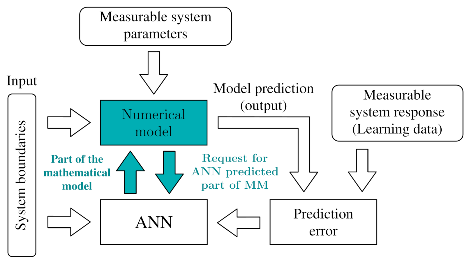
System boundaries are supplied to the ANN, which predicts the assigned part of the mathematical model. System boundaries alongside with an ANN’s output are provided to the numerical model. The numerical model computes the predicted system output. At the learning phase, the predicted output error is used to calculate the proper weights and biases of the ANN. When there is a necessity (e.g., a function is needed to obtain model prediction), IMANN is implemented in such a way that the numerical model sends a request for a part of the mathematical model to ANN with additional parameters (e.g., state of the model, coordinates etc.) Such an approach allows for an interaction between the numerical model and ANN. It should be noted that this is not limited to one request, i.e., the numerical model can request the ANN’s prediction multiple times while producing one output. The proposed approach to a prediction problem is graphically presented in Figure 2. The general approach to developing the IMANN network for any existing numerical model is performed as follows. Having a numerical model , where are the system boundaries and parameters, define a part of the model which will be substituted by an ANN prediction. In place of that part, insert a call to the ANN with input as , where is a vector of all ANN’s input, which will contain selected variables from as well as from variables known by the numerical model during computation. Add ANN as an input to the numerical model. The described algorithm will be further addressed as . The selection of weights and biases is performed by an evolutionary algorithm, which was suggested in the literature for grey-box models [30] but not treated in much detail. Every individual is a representation of one network, i.e., its weights and biases are in the form of a vector. The fitness function is a measure of the discrepancy between a IMANN’s output and a modeled system.
3.2. Learning Process
To train the IMANN, the Covariance Matrix Adaptation-Evolution Strategy (CMA-ES) algorithm is chosen. The CMA-ES algorithm was introduced in [49]. It is an effective and flexible algorithm, which is ideally suited to IMANN learning, where the problem taken under consideration can have different degrees of dimensionality. Here, the dimensionality of the problem is the number of weights and biases in the IMANN. To train the IMANN, the CMA-ES uses a vector made from the network’s weights and biases. The CMA-ES optimizes the vector values based on the error obtained on the training data. Details about the objective function are discussed in the following section. Open-source implementation of CMA-ES in Python was adopted for evolutionary weights adjustments [50].
3.3. Learning Algorithm
- 1.
- Having an empirical dataset D of a N system’s input () and output () paired vectors, define a function which divides the dataset D into training and test data sets— and .
- 2.
- Having a numerical model M and neural network , define a function IMANN(M,) that combines the M and into IMANN.
- 3.
- For a given CMA-ES, optimization parameters initialize the CMA-ES optimization algorithm.
- 4.
- Perform one optimization step for optimization of the weights and biases vector based on a fitness function dependent on the and .
- 5.
- For every solution check squared error made on () and (), save the lowest, throughout whole optimization, value of and the corresponding solution .
- 6.
- Repeat steps 4 and 5 until one of the optimization’s stopping criteria is satisfied.
The above steps in the form of pseudocode are presented in Algorithm 1. Using the squared values of training and test errors is a way to avoid overfitting.
| Algorithm 1 IMANN training process |
| Require: Empirical dataset , CMA-ES optimization parameters , numerical model M |
| 1: |
| 2: // Divide data to training and test sets |
| 3: CMAoptimizer = InitializeCMA // Initialize optimizer |
| 4: do |
| 5: NextGeneration(CMAoptimizer) |
| 6: // Get current population |
| 7: for do |
| 8: // Initialize network from candidate’s weights vector |
| 9: // Initialize IMANN as an integration of the numerical model and the ANN |
| 10: |
| 11: setCandidateFitness(, ) |
| 12: |
| 13: |
| 14: if then |
| 15: |
| 16: save() |
| 17: end if |
| 18: end for |
| 19: while !stopCondition(CMAoptimizer) |
The difference between the PINN and the IMANN training scheme is the usage of models output. In PINN’s learning, the physical model is a part of the neural network and, therefore, is treated as an activation function used to backpropagate the error. Additionally, fulfillment of the corresponding PDE is a part of the optimization. In the IMANN, the part of the solution proposed by the ANN is provided to the numerical model. In terms of fulfilling the PDE, IMANN relies on the numerical model to provide a physically correct prediction.
3.4. This Study
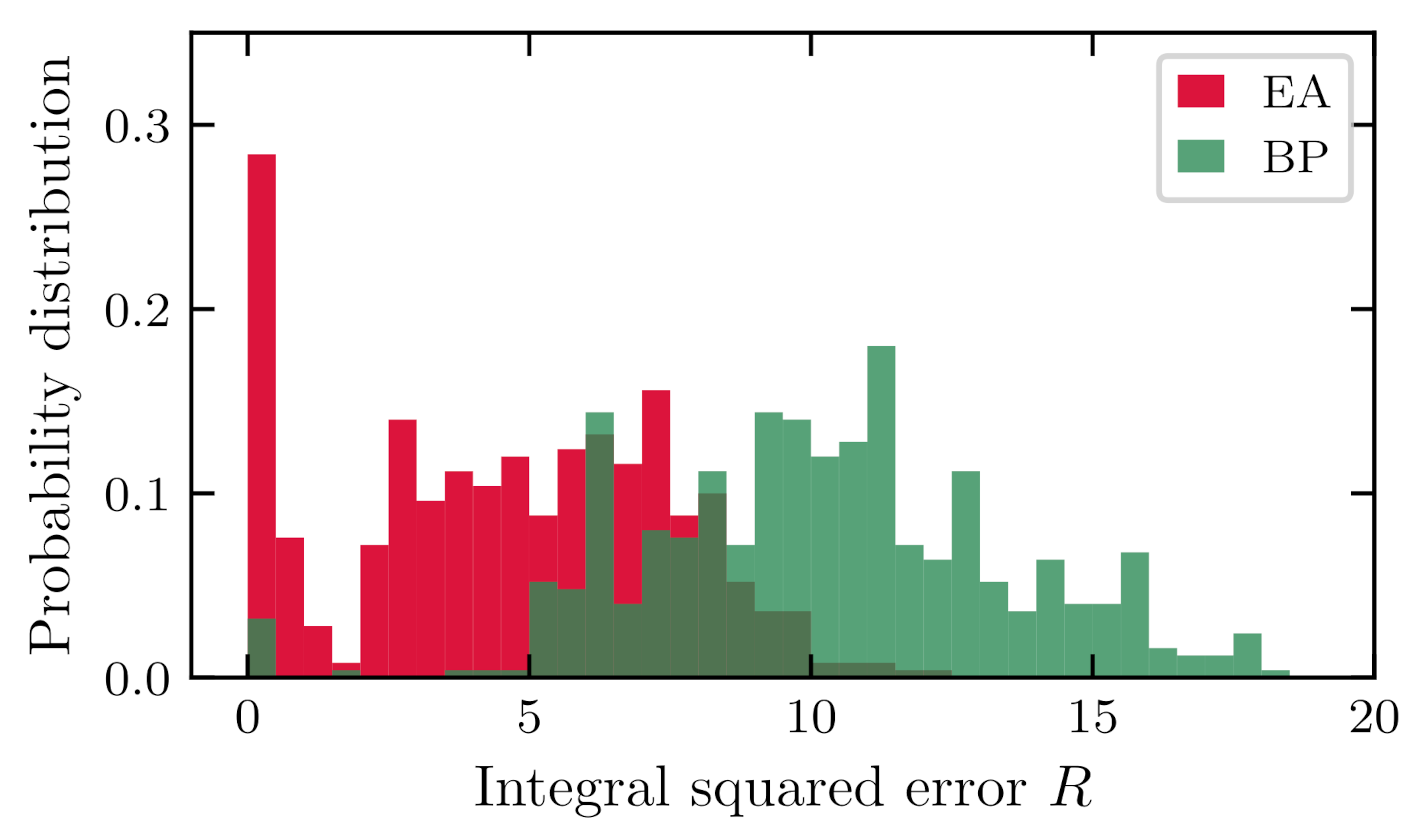
Choosing an EA as a primary optimization technique in the grey-box model comes from two factors. First, introduced earlier in this section, the ability to adjust weights based on a full function predicted by an ANN without the knowledge of the error in each point. Second, the BP algorithm uses derivatives to improve the prediction. Treating the model as an activation function in the last neuron can be poorly conditioned or impossible to solve in specific applications. As a simple example, estimating a constant a in the equation is used. We use two datasets consisting of 20 and 100 points. In both, every fifth point is assigned to the test set (overall 20%). Estimation is performed with the EA and BP algorithms for 500 attempts. The error estimation procedure is described at the beginning of Section 5. Histograms are presented in Figure 3 and Figure 4. For both datasets, the distribution of errors made by the EA’s approach is smaller. The EA and BP approaches struggle with the ambiguous nature of the function - for the finite amount of uniformly distributed data points generated using a trigonometric function, one can find a different function of the same type but with a higher frequency that will have the same function values in provided data points. The BP algorithm additionally has a problem with the last activation function derivative, which is equal to . Such derivative stops the BP algorithm in a local minimum, if the initial weights are not chosen close enough to a good solution. Since the ambiguity of many real problems can lead to unreal models, the parameters proposed by the IMANN should be monitored. In real applications, physical constraints should be added, such as boundaries for the parameters imposed on the ANN output or in the form of additional error terms during learning.
4. Benchmarking Functions
Every system’s output, physical or theoretical, depends on its boundaries (inputs) and characteristics (adaptable parameters). Mathematical models are functions that try to reflect real system behavior. Mathematical models are often based on assumptions and empirical parameters due to the gap in existing knowledge regarding the phenomena. The simplifications in problem formulation results in the discrepancy between the model and the real system outputs. The difference can dissolve only for hypothetical cases where the system output is described by mathematical equations and well-defined.
Every function can be treated as a system, and any arbitrary function can be treated as its mathematical model. The concept of IMANN strives to be reliable and applicable to any system: physical, economic, biological, or social, only when a part of this system can be represented in a mathematical form. To be able to represent a wide range of possible applications, benchmark functions were employed as a representation of the system. The system’s inputs () and measurable outputs () correspond to the inputs and outputs of benchmarking functions. The ANN predicts a part of the system, and the numerical model calculates the rest of it. From the model’s view, the ANN’s prediction is a parameter or one of the model’s equations. Values calculated by the benchmarking functions represent the measurable system outputs. If the subfunction values predicted by the ANN had the same value as calculated from the extracted part of the benchmark function, this would represent a perfect match between the IMANN and the system output. If the real system output differs from the predicted one, the IMANN will be forced to improve the weights and biases.
Functions
To test the IMANN, two benchmarking functions are used. Typical test functions used in optimization problems were used. One polynomial function—Styblinski-Tang function—for a one-dimensional input and Rosenbrock function for two dimensions. The chosen polynomial function is given by formula:
the two-dimensional Rosenbrock function is given by:
In the case of polynomial functions, eight formulations of mathematical models are used, four with one subfunction and four with two subfunctions. The difference between the formulations lies only in the form and number of the subfunctions. Model formulations with one subfunction are given by the following equations:
where and are subfunctions, and is the i-th model function. We have chosen the formulations to distribute the complexity of prediction between ANN and numerical model in different scenarios. Equation (3a) is a case where ANN is responsible for a very simple task, while Equation (3d) results in a complexity similar to the predicting a value of Equation (1). For a perfect match with the modeled benchmarking function, the subfunctions should be functions of x in the form:
The polynomial function’s model formulations with two subfunctions are defined as:
where , and are subfunctions. The idea behind choosing different formulations is the same as for Equation (3a–d). All model functions are defined in the domain . Ideally, the subfunctions should be functions of x in the form:
In the case of the Rosenbrock function, the model formulation is defined in and is given by:
where and ideally are subfunctions of x and y in the form of:
The ANN in the grey-box model is responsible for predicting the value of all subfunctions mentioned above and provides them into the model. The ANN is learned with the difference between the model output and the data generated from a benchmarking function in n sample points , from which are training data points, and are test data points. is the vector of weights and biases of a neural network. The learning process is performed by an evolutionary algorithm, here with the use of a CMA-ES library for Python as explained in Section 3.2. The vector , which fully describes one network, is optimized by an optimization algorithm based on the fitness value:
and the best network is chosen based on the whole dataset according to:
The dimensionality of the optimization of the fully connected network for the considered problem can be expressed with the following formula:
where D is the optimization dimensionality, k is the number of hidden layers, is the number of neurons in the i-th hidden layer and and are the input and output dimensionality, respectively. For instance, the IMANN architecture for the polynomial prediction with one subfunction, the dimensionality of the optimization problem is equal to 47. The computational complexity of the CMA-ES algorithm is at least . Every candidate solution consists of calling ANN for output, which is negligible, and a model function call. Assuming that a numerical model is a unit operation and runs at , the overall computational complexity would be . If computational complexity of a numerical model is dependent on some parameter ℓ and is equal to with some unit operation, the overall computational complexity would be .
5. Results
To quantify the difference between the benchmark function’s output and the predicted value, the integral of the squared error is used as an accuracy indicator:
The integral in Equation (12) is computed with eighty points per dimension Gauss-Legendre quadrature. The IMANN is compared to the DNN implemented with the use of the TensorFlow library [51]. The DNN learns in a standard way, treating the system as a black box. To neglect the stochastic error in the computations, one hundred attempts were performed for the IMANN and the DNN, for every numerousness of the dataset. The mean value of R from these 100 attempts is represented as
For both networks, the training to test dataset numerousness ratio was 7:3. The training set was chosen randomly for each attempt from the same dataset. The best network was chosen according to the algorithm described in the Section 3.3, and an R value was evaluated. An R value was not used for choosing the best network, because it cannot be estimated in real applications. R is used because it is a better measure of a network’s performance than the error made on the training and test data sets. The term ANN is used when referring to ANN part of IMANN and DNN for a typical ANN implementation.
5.1. Architecture
The implementation of the IMANN has a feedforward architecture consisting of fully connected layers with the last two layers called the part of the model layer (PM layer) and the model layer. In the input layer, the number of neurons corresponds to the conditions in which the system is located. Further layers are standard hidden layers. The number of layers and the number of neurons contained therein are selected according to the complexity of the problem modeled by the network. The next layer is the mentioned PM layer, where the number of neurons corresponds to the number of replaced parts of the model. The output from that layer multiplied by the weights is directly entered into the model layer. The numerical model also receives all arguments that were supplied to the network’s input, alongside the system parameters. The calculated numerical model result is the final output of the IMANN. Schematically, the IMANN’s architecture is presented in Figure 5. The implementation of the DNN was done by using the TensorFlow 1.12.0 library. The neural network is trained with the backpropagation algorithm using batches of size equal six. The optimizer used is Adam with default settings. For both DNN and IMANN, Bent Identity activation functions are used in all neurons. The IMANN’s architectures for problems (4a–d), (6a–d) and (8) were 1-5-5-1, 1-5-5-2 and 2-5-5-2, respectively. DNN’s architectures for problems (1) and (2) were 1-32-16-16-1 and 2-32-32-16-1, respectively. Architectures, as well as activation functions, were adjusted by trial and error for the best performance.
In terms of Figure 2 and Figure 5, x or () are the “System boundaries”, i.e., inputs, to both the numerical model and the ANN. “Measurable system parameters” can be viewed as any of the constants present in the corresponding problem. The “request for ANN predicted part of mathematical model” is the calling of ANN for a prediction, here without providing any additional inputs. “Part of the mathematical model” is the corresponding subfunction provided by the ANN. The model prediction is the value of , and the “measurable system response” is a real value corresponding to the input.
5.2. Statistical Testing
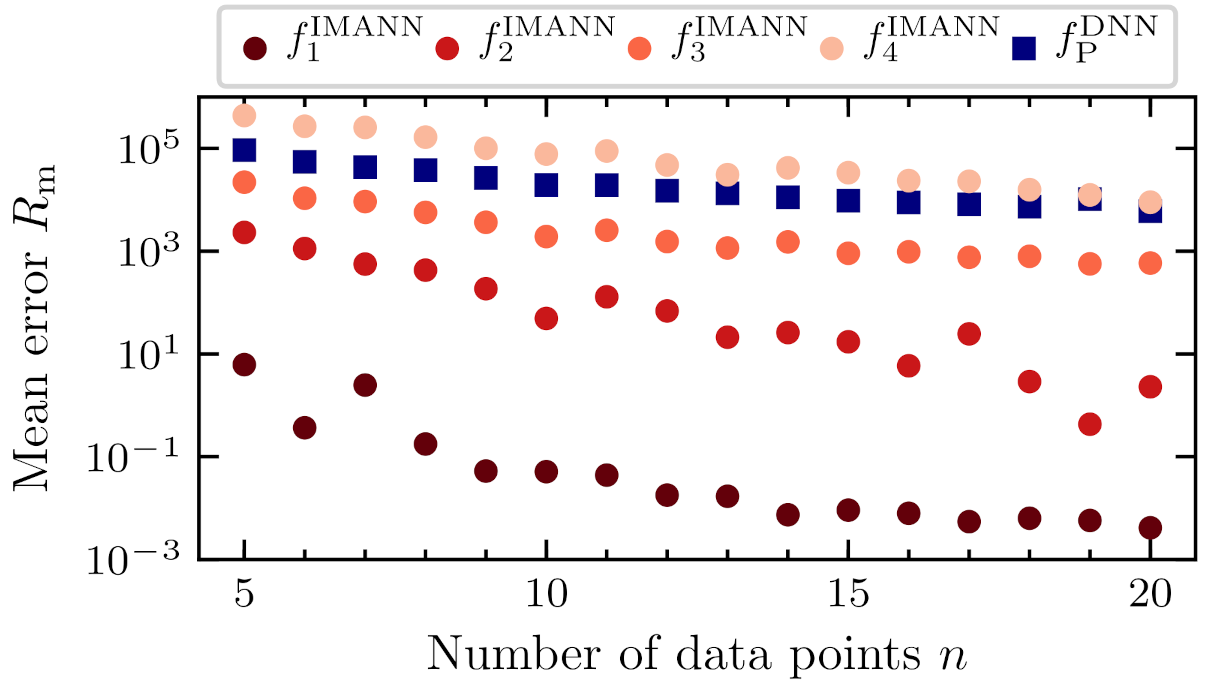
The first paragraph covers the statistical comparison of IMANN and DNN algorithms over the case problems defined in Section 4. One must keep in mind that all IMANN implementations (i.e., IMANN’s designed for every model formulation –) were treated as if they were different algorithms. The algorithm and its prediction are represented with the same notation—subscript denotes problem (modeled function), and superscript indicates implementation (DNN or IMANN)—and the meaning is clear based on the context. Every algorithm has to minimize the errors of problems defined as a pair of functions and the dataset’s size. Errors were defined according to Equation (12). Means of errors obtained for the problems for every dataset are presented in Table 1 and graphically in Figure 6 and Figure 7. Statistical testing was performed according to the guidelines indicated in Derrac et al. [52]. The Quade test was used for testing the null hypothesis, asserting the equality of medians between the distribution of errors made by different algorithms on overall problems to test if the algorithms differ significantly from each other [52]. Average Quade rankings are presented in Table 2. Quade statistic distributed according to F-distribution with 8 and 120 degrees of freedom is equal to 46.624. p-value computed by Quade Test is 2.6476 × 10⁻³³, which rejects the null hypothesis and, in the result, states that the algorithms’ performance differs significantly. The next step is to test the hypothesis of equality between all pairs of algorithms [52]. For this step, the Shaffer post-hoc procedure is used. z-values, associated p-values and adjusted p-values for are presented in Table 3. The z-value is used to determine the p-value from the normal distribution . Adjusted p-value takes into account the accumulation of errors made by multiple comparisons. If adjusted p-value is less than the value, the algorithms’ performance differs with the level of significance equal to . In Table 3, significant differences are separated with an additional line. It can be seen in the Table 3 that when the ANN in the IMANN has to predict non-complex function (model formulations , , , and ), the grey box outperforms the DNN, which is indicated by the low adjusted p-value between the corresponding pairs. For more complex problems (model formulations , and ) the difference is not significant. Another dependency worth noticing in Table 3 is that the number of parameters does not change the performance significantly (hypotheses of equality between pairs and , and , and and and cannot be rejected with 5% significance level).
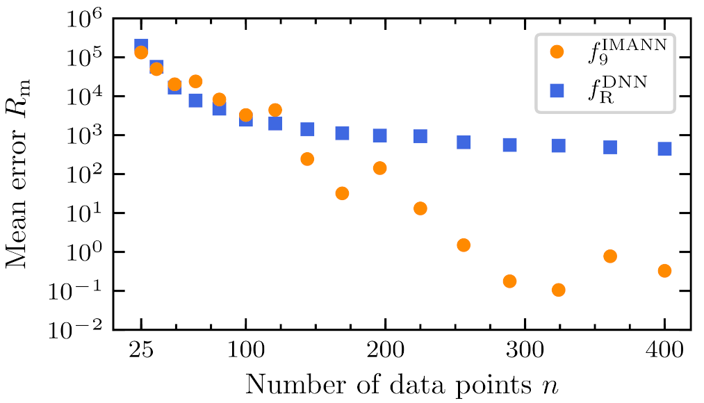
Another test was performed to test the differences between standard DNN and IMANN formulations for Rosenbrock with two-dimensional input. Mean errors over one hundred trials obtained for every different dataset numerousness are presented in Table 4 and graphically in Figure 8. To compare these two formulations, Wilcoxon procedure was employed, as proposed by Derrac et al. [52]. Wilcoxon ranks are presented in Table 5. The lower of the two should be less than or equal to the critical value obtained from the Wilcoxon distribution. The critical value obtained from Wilcoxon distribution for 16 degrees of freedom and the level of significance is equal to 29, which is lower that 57; therefore, the null hypothesis of equality of means cannot be rejected. Still, a great increase of IMANN’s performance with enough data points presented in Figure 8, shows promising potential. High mean error value for IMANN, when the data numerousness is lower than 11 points per input dimension, is caused by 2 trials per 100 with very high error value. This problem may be addressed with a different learning approach.
5.3. Examples of Prediction
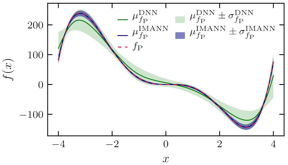
To illustrate the difference between the prediction of IMANN and DNN, an IMANN implementation for and is chosen. Mean with one standard deviation distance of the predicted parameter for is presented in Figure 9. One can see that the highest deviation is close to , where the term vanishes and thus does not count in error significantly. This observation is especially significant when one wants to interpret the value of the parameter predicted by the IMANN. In a domain where the parameter’s impact on system behavior is insignificant, its value should be treated as obtained with very low accuracy. Same figure type for two parameters , for formulation is presented in Figure 10. Here the deviation between ideal parameters’ values and predicted by the IMANN is very high. The reason for such a difference is the ambiguity that arises when two parameters are predicted. In the Figure 11 the blue line and the blue area indicates the mean prediction made by the IMANN and one standard deviation area, the green line and the green area indicates the prediction made by the DNN and one standard deviation area while the red line is the . As can be seen, even though IMANN-predicted parameters have formed different than expected, the resulting prediction of the function is highly accurate. This implies two important remarks. First, interpreting subfunctions’ values provided by IMANN should be checked for ambiguity, and second, proper constraints put on subfunctions’ values can reduce the number of ambiguous solutions. The constraints can be introduced by adding an additional penalty term in the error function during training. The penalty can correspond to subfunction values in specific points, range, or even shape described with derivative (e.g., monotonicity).
Comparison between IMANN and DNN mean predictions of Rosenbrock function for two different dataset numerousness are presented in Figure 12 for 36 data points (25 training points) and in Figure 13 for 256 data points (179 training points). For a low number of data points, the maximum discrepancy between prediction and original function for IMANN is of one order of magnitude lower than for DNN. For a higher number of points, the advantage of IMANN over DNN is greater, reaching the difference of two orders of magnitude.
6. Discussion
From the idea of the IMANN, one can see that by decreasing the load on the ANN part to zero in the IMANN will result in the IMANN’s prediction performance equal to the model (see Figure 2). In the proposed benchmarking case, the numerical model performance is perfect because we already know the form of the subfunctions. In real applications, finding even such a simple thing as the constant fitting parameters might be a problem.
Generalized computations from Section 5 prove that the IMANN can achieve higher performance than the DNN, as presented in Table 3. Gray-box approach is better than black-box when the complexity of subfunctions is lower than the complexity of a predicted function (see the upper part of Table 3). There was no significant difference when one and two subfunctions were modeled by the IMANN with similar complexity of subfunctions (see the lower part of Table 3. Therefore, the IMANN can improve the mathematical model’s performance by modeling its oversimplified, uncertain or missing parts, that are responsible for the discrepancy between the numerical model’s prediction and the modelled system.. The power of artificial neural network is utilized only for the problem part that cannot be solved accurately any other way. Such an approach reduces the complexity of a problem that is solved by an ANN, resulting in better prediction, especially with a small number of learning data points. The obtained results indicate great potential in the integration of mathematical models and artificial neural networks.
There are two major limitations of the IMANN. Since learning requires to run a numerical algorithm for each training data point each time a set of weights is tested, a reasonable learning time may not be obtained with computationally heavy numerical models. A second limitation arises from the fact that a problem of providing a part of the model by the ANN can become ambiguous, which can result in an unphysical or irrational form of subfunctions without additional control. A proposed way to keep ANN outputs physical is to impose additional constraints by adding penalty terms in . As for results provided in this paper, this topic is not studied.
7. Practical Application in Solid Oxide Fuel Cells Modeling
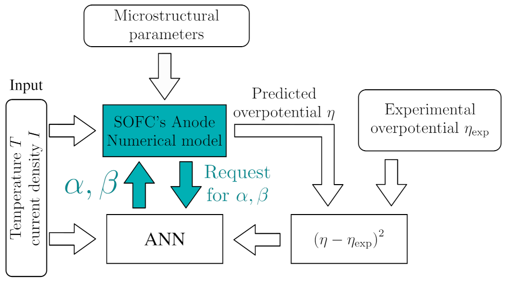
Microscale modeling of Solid Oxide Fuel Cell’s (SOFC) anode comes with a highly difficult problem of modeling a multistep electrochemical reaction between oxygen ions and hydrogen. The reaction occurs in the so-called triple phase boundary (TPB) and is a basis of SOFC’s operation. The equation which describes the reaction has empirical parameters that have to be estimated or fitted into the solution. Simplified equation (without elaborating the preexponential term ) takes the form described by the Butler-Volmer formula:
where is the volumetric exchange current density (), is the exchange current density (), F = 96,485.3415 s A/mol is the Faraday constant, T is the temperature (), and are the charge transfer coefficients (1) that are obtained by fitting to the experimental data [53], is activation overpotential (). Detailed mathematical model of SOFC’s anode phenomena can be found elsewhere (e.g., [54]).
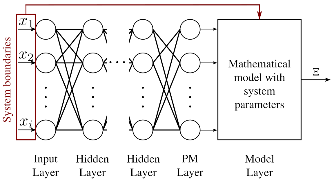
The Butler-Volmer equation comes with three empirical parameters—, and , for which the values and the functional dependence from microstructural and system parameters is unknown [55]. Here, an ANN is employed to provide and values as functions of temperature T (K) and current density I () for numerical model of the anode. The architecture is schematically presented in Figure 14.
Data available in the literature [56] was used as a source of microstructural parameters, typically used charge transfer coefficients’ values and both training and test datasets. Training set consisted of twelve data points, six for and six for . The test set was made of six data points for temperature .
The ANN’s architecture contains one hidden layer consisting of three neurons with Bent Identity activation functions. The output layer contains two neurons—one for and one for charge transfer coefficients—with SoftPlus activation functions, as values of charge transfer coefficients should be positive. The output of activation functions was directly provided to the numerical model. The inputs to the ANN were temperature and current density.
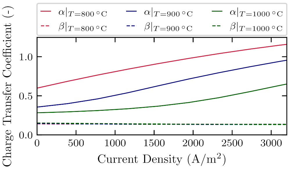
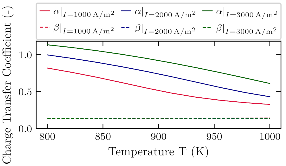
To check if the IMANN architecture provides values that are physically feasible, it is shown what is the proposed functional form of charge transfer coefficients in dependence from current density, Figure 15, and temperature, Figure 16. In Figure 15 values of both and charge transfer coefficients are presented as functions of current density for three different operating temperatures. It can be seen that the value proposed by the ANN changes nonlinearly with the current density and is increasing monotonically. In Figure 16 charge transfer coefficients are presented as functions of temperature for three different current densities. The value changes nonlinearly with the temperature and is decreasing monotonically. The value is practically independent from both temperature and current density. Values of charge transfer coefficients proposed by the ANN are close to the ones frequently used in the literature. Researchers in the literature propose different values for charge transfer coefficents. For and , one can find values in the ranges and , corespondingly [55,57,58].
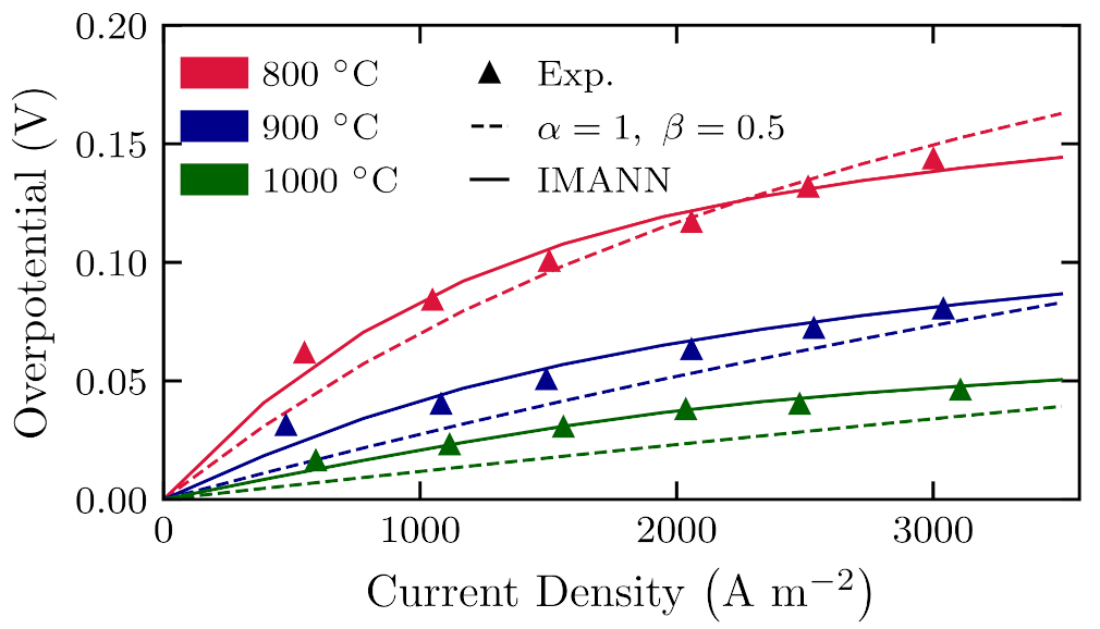
To see the improvement of the overall model, IMANN architecture is compared to the model with typically used charge transfer coefficient values. In the Figure 17 overpotential of the anode versus current density is presented for three different temperatures taken from the literature [56]. Experimental data points are marked as symbols, the standard model is represented as a dashed line, and the proposed method is represented as a solid line. It can be seen that for all data points—both training and test—hybrid model outperforms the classical model in terms of agreement with experimental measurements.
8. Conclusions
The present paper introduced a framework for integrating a classical mathematical model and an artificial neural network, using an evolutionary algorithm to limit the required dataset. The methodology can be applied to any system only if a part of it can be expressed in the form of mathematical equations. The combination of an artificial neural network and a classical mathematical model is interactive, expressed in the possibility to exchange information between a numerical model and ANN as a numerical model’s request and ANN’s response. The Interactive Mathematical Model-Artificial Neural Network was employed to predict several benchmark functions’ values when given a different number of training data. Problems presented in this work were narrowed to theoretical cases with limited complexity compared to real applications. However, the proposed approach can be applied to simulate any system for which the mathematical model is incomplete and a limited dataset of experimental data is available. This situation is widespread in engineering. A practical application in the Solid Oxide Fuel Cell modeling was successfully presented, in which parameters provided by ANN were physically feasible and model prediction was improved. Current limitations include computational complexity due to the use of the derivative-free method for problems of high dimensionality, which requires to call a potentially numerical-heavy numerical model thousands of times. This problem can be addressed by searching for the most optimal optimization method in this application. Another limitation that was described corresponds to the specific problem, not to the IMANN idea. Therefore, it has to be controlled during application by forcing physical and realistic values and comparing the proposed by the IMANN solution to the available experimental or literature data. In future work, the problem of dimensionality should be addressed, i.e., making the possibility of using ANN architectures with a greater number of neurons and layers. More complicated IMANN architectures, including multiple neural networks assigned to different model parts, convolutional neural networks to reduce the number of optimized coefficients or feedback loops (like recurrent ANNs) to achieve additional information for ANN, like the model’s state, can be investigated.
Author Contributions
Conceptualization, G.B.; methodology, S.B., M.G., G.B.; software, S.B., M.G.; validation, S.B., M.G.; formal analysis, S.B.; investigation, S.B., M.G.; resources, M.G., S.B.; data curation, S.B.; writing—original draft preparation, G.B., S.B.; writing—review and editing, G.B., S.B.; visualization, S.B.; supervision, G.B.; project administration, G.B.; funding acquisition, G.B. All authors have read and agreed to the published version of the manuscript.
Funding
This work was supported by the Foundation for Polish Science under FIRST TEAM program No. First TEAM/2016-1/3 co-financed by the European Union under the European Regional Development Fund. The authors acknowledge the support of the Initiative for Excellence—Research University Project at AGH University of Science and Technology and AGH Grant No. 16.16.210.476.
Institutional Review Board Statement
Not applicable.
Informed Consent Statement
Not applicable.
Data Availability Statement
All data available on request.
Acknowledgments
Matplotlib Python library was used for data visualization [59].
Conflicts of Interest
The authors declare no conflict of interest. The funders had no role in the design of the study; in the collection, analyses, or interpretation of data; in the writing of the manuscript, or in the decision to publish the results.
References
- Nikzad, M.; Movagharnejad, K.; Talebnia, F. Comparative Study between Neural Network Model and Mathematical Models for Prediction of Glucose Concentration during Enzymatic Hydrolysis. Int. J. Comput. Appl. Technol. 2012, 56, 43–48. [Google Scholar] [CrossRef]
- Tan, W.C.; Iwai, H.; Kishimoto, M.; Brus, G.; Szmyd, J.S.; Yoshida, H. Numerical analysis on effect of aspect ratio of planar solid oxide fuel cell fueled with decomposed ammonia. J. Power Sources 2018, 384, 367–378. [Google Scholar] [CrossRef]
- Brus, G.; Raczkowski, P.F.; Kishimoto, M.; Iwai, H.; Szmyd, J. A microstructure-oriented mathematical model of a direct internal reforming solid oxide fuel cell. Energy Convers. Manag. 2020, 213, 112826. [Google Scholar] [CrossRef]
- Brus, G.; Iwai, H.; Otani, Y.; Saito, M.; Yoshida, H.; Szmyd, J.S. Local Evolution of Triple Phase Boundary in Solid Oxide Fuel Cell Stack After Long-term Operation. Fuel Cells 2015, 15, 545–548. [Google Scholar] [CrossRef]
- Chalusiak, M.; Nawrot, W.; Buchaniec, S.; Brus, G. Swarm Intelligence-Based Methodology for Scanning Electron Microscope Image Segmentation of Solid Oxide Fuel Cell Anode. Energies 2021, 14, 3055. [Google Scholar] [CrossRef]
- Brus, G.; Iwai, H.; Szmyd, J.S. An Anisotropic Microstructure Evolution in a Solid Oxide Fuel Cell Anode. Nanoscale Res. Lett. 2020, 15, 427. [Google Scholar] [CrossRef] [PubMed]
- Chalusiak, M.; Wrobel, M.; Mozdzierz, M.; Berent, K.; Szmyd, J.S.; Brus, G. A numerical analysis of unsteady transport phenomena in a Direct Internal Reforming Solid Oxide Fuel Cell. Int. J. Heat Mass Transf. 2019, 131, 1032–1051. [Google Scholar] [CrossRef]
- Mozdzierz, M.; Berent, K.; Kimijima, S.; Szmyd, J.S.; Brus, G. A Multiscale Approach to the Numerical Simulation of the Solid Oxide Fuel Cell. Catalysts 2019, 9, 253. [Google Scholar] [CrossRef] [Green Version]
- Andonie, R. Extreme Data Mining: Inference from Small Datasets. Int. J. Comput. Commun. Control 2010, 5, 280–291. [Google Scholar] [CrossRef] [Green Version]
- Cataron, A.; Andonie, R. How to infer the informational energy from small datasets. In Proceedings of the 2012 13th International Conference on Optimization of Electrical and Electronic Equipment (OPTIM 2012), Brasov, Romania, 24–26 May 2012; pp. 1065–1070. [Google Scholar] [CrossRef]
- Shaikhina, T.; Khovanova, N.A. Handling limited datasets with neural networks in medical applications: A small-data approach. Artif. Intell. Med. 2017, 75, 51–63. [Google Scholar] [CrossRef]
- Micieli, D.; Minniti, T.; Evans, L.M.; Gorini, G. Accelerating Neutron Tomography experiments through Artificial Neural Network based reconstruction. Sci. Rep. 2019, 9, 2450. [Google Scholar] [CrossRef] [PubMed]
- Simard, P.Y.; Steinkraus, D.; Platt, J.C. Best practices for convolutional neural networks applied to visual document analysis. In Proceedings of the Seventh International Conference on Document Analysis and Recognition, Edinburgh, UK, 6 August 2003; pp. 958–963. [Google Scholar] [CrossRef]
- Baird, H.S.; Bunke, H.; Yamamoto, K. (Eds.) Document Image Defect Models. In Structured Document Image Analysis; Springer: Berlin/Heidelberg, Germany, 1992; pp. 546–556. [Google Scholar] [CrossRef]
- Simard, P.; Victorri, B.; LeCun, Y.; Denker, J. Tangent Prop—A formalism for specifying selected invariances in an adaptive network. In Proceedings of the Advances in Neural Information Processing Systems (NIPS), Denver, CO, USA, 2–5 December 1991; pp. 895–903. [Google Scholar]
- Rozsa, A.; Rudd, E.M.; Boult, T.E. Adversarial Diversity and Hard Positive Generation. In Proceedings of the 2016 IEEE Conference on Computer Vision and Pattern Recognition Workshops (CVPRW), Las Vegas, NV, USA, 26 June–1 July 2016; pp. 410–417. [Google Scholar] [CrossRef] [Green Version]
- Lemley, J.; Bazrafkan, S.; Corcoran, P. Smart Augmentation Learning an Optimal Data Augmentation Strategy. IEEE Access 2017, 5, 5858–5869. [Google Scholar] [CrossRef]
- Edelsbrunner, H.; Letscher, D.; Zomorodian, A. Topological persistence and simplification. In Proceedings of the 41st Annual Symposium on Foundations of Computer Science, Redondo Beach, CA, USA, 12–14 November 2000; pp. 454–463. [Google Scholar] [CrossRef]
- Adams, H.; Emerson, T.; Kirby, M.; Neville, R.; Peterson, C.; Shipman, P.; Chepushtanova, S.; Hanson, E.; Motta, F.; Ziegelmeier, L. Persistence Images: A Stable Vector Representation of Persistent Homology. J. Mach. Learn. Res. 2017, 18, 1–35. [Google Scholar]
- Adcock, A.; Carlsson, E.; Carlsson, G. The ring of algebraic functions on persistence bar codes. Homol. Homotopy Appl. 2016, 18, 381–402. [Google Scholar] [CrossRef] [Green Version]
- Towell, G.G.; Shavlik, J.W. Knowledge-based artificial neural networks. Artif. Intell. 1994, 70, 119–165. [Google Scholar] [CrossRef]
- Su, H.T.; Bhat, N.; Minderman, P.; McAvoy, T. Integrating Neural Networks with First Principles Models for Dynamic Modeling. IFAC Proc. Vol. 1992, 25, 327–332. [Google Scholar] [CrossRef]
- Wang, F.; Zhang, Q.j. Knowledge-based neural models for microwave design. IEEE Trans. Microw. Theory Tech. 1997, 45, 2333–2343. [Google Scholar] [CrossRef]
- Bandler, J.W.; Ismail, M.A.; Rayas-Sanchez, J.E.; Zhang, Q.-J. Neuromodeling of microwave circuits exploiting space-mapping technology. IEEE Trans. Microw. Theory Tech. 1999, 47, 2417–2427. [Google Scholar] [CrossRef]
- Na, W.; Feng, F.; Zhang, C.; Zhang, Q. A Unified Automated Parametric Modeling Algorithm Using Knowledge-Based Neural Network and l1 Optimization. IEEE Trans. Microw. Theory Tech. 2017, 65, 729–745. [Google Scholar] [CrossRef]
- Psichogios, D.C.; Ungar, L.H. A Hybrid Neural Network-First Principles Approach to Process Modeling. AIChE J. 1992, 38, 1499–1511. [Google Scholar] [CrossRef]
- Hagge, T.; Stinis, P.; Yeung, E.; Tartakovsky, A.M. Solving differential equations with unknown constitutive relations as recurrent neural networks. arXiv 2017, arXiv:1710.02242. [Google Scholar]
- De Veaux, R.D.; Bain, R.; Ungar, L.H. Hybrid neural network models for environmental process control: (The 1998 Hunter Lecture). Environmetrics 1999, 10, 225–236. [Google Scholar] [CrossRef]
- Acuña, G.; Cubillos, F.; Thibaule, J.; Latrille, E. Comparison of methods for training grey-box neural network models. Comput. Chem. Eng. 1999, 23, S561–S564. [Google Scholar] [CrossRef]
- Oliveira, R. Combining first principles modelling and artificial neural networks: A general framework. Comput. Chem. Eng. 2004, 28, 755–766. [Google Scholar] [CrossRef]
- Cubillos, F.A.; Alvarez, P.I.; Pinto, J.C.; Lima, E.L. Hybrid-neural modeling for particulate solid drying processes. Powder Technol. 1996, 87, 153–160. [Google Scholar] [CrossRef]
- Piron, E.; Latrille, E.; René, F. Application of artificial neural networks for crossflow microfiltration modelling: “Black-box” and semi-physical approaches. Comput. Chem. Eng. 1997, 21, 1021–1030. [Google Scholar] [CrossRef]
- Vieira, J.A.; Mota, A.M. Combining first principles with grey-box approaches for modelling a water gas heater system. In Proceedings of the 20th IEEE International Symposium on Intelligent 652 Control, ISIC’05 and the 13th Mediterranean Conference on Control and Automation, MED’05, Limassol, Cyprus, 27–29 June 2005; pp. 1137–1142. [Google Scholar] [CrossRef]
- Romijn, R.; Özkan, L.; Weiland, S.; Ludlage, J.; Marquardt, W. A grey-box modeling approach for the reduction of nonlinear systems. J. Process Control 2008, 18, 906–914. [Google Scholar] [CrossRef]
- Chaffart, D.; Ricardez-Sandoval, L.A. Optimization and control of a thin film growth process: A hybrid first principles/artificial neural network based multiscale modelling approach. Comput. Chem. Eng. 2018, 119, 465–479. [Google Scholar] [CrossRef]
- Cen, Z.; Wei, J.; Jiang, R. A grey-box neural network based identification model for nonlinear dynamic systems. In Proceedings of the 4th International Workshop on Advanced Computational Intelligence (IWACI 2011), Wuhan, China, 19–21 October 2011; pp. 300–307. [Google Scholar] [CrossRef]
- Lagaris, I.E.; Likas, A.; Fotiadis, D.I.F. Artificial Neural Networks for Solving Ordinary and Partial Differential Equations. IEEE Trans. Neural Netw. 1998, 9, 987–1000. [Google Scholar] [CrossRef] [Green Version]
- Raissi, M.; Perdikaris, P.; Karniadakis, G.E. Physics-informed neural networks: A deep learning framework for solving forward and inverse problems involving nonlinear partial differential equations. J. Comput. Phys. 2019, 378, 686–707. [Google Scholar] [CrossRef]
- Parish, E.J.; Duraisamy, K. A paradigm for data-driven predictive modeling using field inversion and machine learning. J. Comput. Phys. 2016, 305, 758–774. [Google Scholar] [CrossRef] [Green Version]
- Shukla, K.; Jagtap, A.D.; Karniadakis, G.E. Parallel Physics-Informed Neural Networks via Domain Decomposition. arXiv 2021, arXiv:2104.10013. [Google Scholar]
- Jagtap, A.D.; Em Karniadakis, G. Extended Physics-Informed Neural Networks (XPINNs): A Generalized Space-Time Domain Decomposition Based Deep Learning Framework for Nonlinear Partial Differential Equations. Commun. Comput. Phys. 2020, 28, 2002–2041. [Google Scholar] [CrossRef]
- Jagtap, A.D.; Kharazmi, E.; Karniadakis, G.E. Conservative physics-informed neural networks on discrete domains for conservation laws: Applications to forward and inverse problems. Comput. Methods Appl. Mech. Eng. 2020, 365, 113028. [Google Scholar] [CrossRef]
- Shukla, K.; Di Leoni, P.C.; Blackshire, J.; Sparkman, D.; Karniadakis, G.E. Physics-Informed Neural Network for Ultrasound Nondestructive Quantification of Surface Breaking Cracks. J. Nondestruct. Eval. 2020, 39, 61. [Google Scholar] [CrossRef]
- Shukla, K.; Jagtap, A.D.; Blackshire, J.L.; Sparkman, D.; Karniadakis, G.E. A physics-informed neural network for quantifying the microstructure properties of polycrystalline Nickel using ultrasound data. arXiv 2021, arXiv:2103.14104. [Google Scholar]
- Ling, J.; Kurzawski, A.; Templeton, J. Reynolds averaged turbulence modelling using deep neural networks with embedded invariance. J. Fluid Mech. 2016, 807, 155–166. [Google Scholar] [CrossRef]
- Wu, J.L.; Xiao, H.; Paterson, E. Physics-informed machine learning approach for augmenting turbulence models: A comprehensive framework. Phys. Rev. Fluids 2018, 7, 1–28. [Google Scholar] [CrossRef] [Green Version]
- Chan, S.; Elsheikh, A.H. A machine learning approach for efficient uncertainty quantification using multiscale methods. J. Comput. Phys. 2018, 354, 493–511. [Google Scholar] [CrossRef] [Green Version]
- Tripathy, R.K.; Bilionis, I. Deep UQ: Learning deep neural network surrogate models for high dimensional uncertainty quantification. J. Comput. Phys. 2018, 375, 565–588. [Google Scholar] [CrossRef] [Green Version]
- Hansen, N.; Ostermeier, A. Adapting arbitrary normal mutation distributions in evolution strategies: The covariance matrix adaptation. In Proceedings of the IEEE International Conference on Evolutionary Computation, Nagoya, Japan, 20–22 May 1996; pp. 312–317. [Google Scholar] [CrossRef]
- Hansen, N.; Akimoto, Y.; Baudis, P. CMA-ES/Pycma on Github. 2019. Available online: https://github.com/CMA-ES/Pycma (accessed on 30 September 2020).
- Abadi, M.; Agarwal, A.; Barham, P.; Brevdo, E.; Chen, Z.; Citro, C.; Corrado, G.S.; Davis, A.; Dean, J.; Devin, M.; et al. TensorFlow: Large-Scale Machine Learning on Heterogeneous Systems. 2015. Available online: https://www.tensorflow.org (accessed on 30 September 2020).
- Derrac, J.; García, S.; Molina, D.; Herrera, F. A practical tutorial on the use of nonparametric statistical tests as a methodology for comparing evolutionary and swarm intelligence algorithms. Swarm Evol. Comput. 2011, 1, 3–18. [Google Scholar] [CrossRef]
- Li, X. Principles of Fuel Cells, 1st ed.; Taylor & Francis: New York, NY, USA, 2006. [Google Scholar]
- Buchaniec, S.; Sciazko, A.; Mozdzierz, M.; Brus, G. A Novel Approach to the Optimization of a Solid Oxide Fuel Cell Anode Using Evolutionary Algorithms. IEEE Access 2019, 7, 34361–34372. [Google Scholar] [CrossRef]
- de Boer, B. SOFC Anode. Hydrogen Oxidation at Porous Nickel and Nickel/Zirconia Electrodes. Ph.D. Thesis, University of Twente, Enschede, The Netherlands, 1998. [Google Scholar]
- Kishimoto, M.; Iwai, H.; Saito, M.; Yoshida, H. Quantitative evaluation of solid oxide fuel cell porous anode microstructure based on focused ion beam and scanning electron microscope technique and prediction of anode overpotentials. J. Power Sources 2011, 196, 4555–4563. [Google Scholar] [CrossRef]
- Marina, O.A.; Pederson, L.R.; Williams, M.C.; Coffey, G.W.; Meinhardt, K.D.; Nguyen, C.D.; Thomsen, E.C. Electrode Performance in Reversible Solid Oxide Fuel Cells. J. Electrochem. Soc. 2007, 154, B452. [Google Scholar] [CrossRef]
- Kawada, T.; Sakai, N.; Yokokawa, H.; Dokiya, M.; Mori, M.; Iwata, T. Characteristics of Slurry-Coated Nickel Zirconia Cermet Anodes for Solid Oxide Fuel Cells. J. Electrochem. Soc. 1990, 137, 3042–3047. [Google Scholar] [CrossRef]
- Hunter, J.D. Matplotlib: A 2D graphics environment. Comput. Sci. Eng. 2007, 9, 90–95. [Google Scholar] [CrossRef]
Figure 1.
The comparison of two approaches to the prediction problem with use of an ANN (a) black box (b) combination of a mathematical model and ANN grey box.
Figure 1.
The comparison of two approaches to the prediction problem with use of an ANN (a) black box (b) combination of a mathematical model and ANN grey box.

Figure 2.
The Interactive Mathematical Modeling-Artificial Neural Network block diagram.

Figure 3.
Error probability distribution comparison between EA and BP algorithms for constant estimation based on 20 data points.
Figure 3.
Error probability distribution comparison between EA and BP algorithms for constant estimation based on 20 data points.

Figure 4.
Error probability distribution comparison between EA and BP algorithms for constant estimation based on 100 data points.
Figure 4.
Error probability distribution comparison between EA and BP algorithms for constant estimation based on 100 data points.

Figure 5.
Architecture schema of the IMANN used in benchmark problems.

Figure 6.
Mean integral squared error for algorithms – and change with numerousness of dataset.

Figure 7.
Mean integral squared error for algorithms – and change with numerousness of data set.

Figure 8.
Mean integral squared error for problems and change with numerousness of data set.

Figure 9.
Mean prediction of a subfunction made by IMANN with indicated one standard deviation region.
Figure 9.
Mean prediction of a subfunction made by IMANN with indicated one standard deviation region.

Figure 10.
Mean predictions and of a and subfunction made by IMANN with indicated one standard deviation and regions.
Figure 10.
Mean predictions and of a and subfunction made by IMANN with indicated one standard deviation and regions.

Figure 11.
Mean predictions and of function with corresponding one standard deviation regions and . IMANN prediction corresponds to formulation , for which mean values of parameters and can be found in Figure 10.
Figure 11.
Mean predictions and of function with corresponding one standard deviation regions and . IMANN prediction corresponds to formulation , for which mean values of parameters and can be found in Figure 10.

Figure 12.
Rosenbrock function prediction with DNN and IMANN for 36 data points. Surfaces correspond to predicted values, wireframe to original function, blue points indicate data points and colormap on the bottom indicates absolute error.
Figure 12.
Rosenbrock function prediction with DNN and IMANN for 36 data points. Surfaces correspond to predicted values, wireframe to original function, blue points indicate data points and colormap on the bottom indicates absolute error.

Figure 13.
Rosenbrock function prediction with DNN and IMANN for 256 data points. Surfaces correspond to predicted value, wireframe to original function, blue points indicate data points and colormap on the bottom indicates absolute error.
Figure 13.
Rosenbrock function prediction with DNN and IMANN for 256 data points. Surfaces correspond to predicted value, wireframe to original function, blue points indicate data points and colormap on the bottom indicates absolute error.

Figure 14.
Architecture schema of the IMANN in application to SOFC’s anode microscale modeling.

Figure 15.
Charge transfer coefficients values proposed by the IMANN versus current density.

Figure 16.
Charge transfer coefficients values proposed by the IMANN versus temperature.

Figure 17.
Overpotential curve comparison between IMANN grey-box model versus experimental data from [56] and numerical model with standard parameters.
Figure 17.
Overpotential curve comparison between IMANN grey-box model versus experimental data from [56] and numerical model with standard parameters.


Table 1.
Mean integral squared error value .
| Dataset | |||||||||
|---|---|---|---|---|---|---|---|---|---|
| 5 | |||||||||
| 6 | |||||||||
| 7 | |||||||||
| 8 | |||||||||
| 9 | |||||||||
| 10 | |||||||||
| 11 | |||||||||
| 12 | |||||||||
| 13 | |||||||||
| 14 | |||||||||
| 15 | |||||||||
| 16 | |||||||||
| 17 | |||||||||
| 18 | |||||||||
| 19 | |||||||||
| 20 |
Table 2.
Average rankings of the algorithms (Quade).
| Algorithm | Ranking |
|---|---|
| 9.000 | |
| 7.331 | |
| 5.581 | |
| 1.000 | |
| 7.669 | |
| 5.294 | |
| 4.125 | |
| 3.000 | |
| 2.000 |
Table 3.
Shaffer Table for .
| Algorithms | z | p | Adjusted p |
|---|---|---|---|
| vs. | |||
| vs. | |||
| vs. | |||
| vs. | |||
| vs. | |||
| vs. | |||
| vs. | |||
| vs. | |||
| vs. | |||
| vs. | |||
| vs. | |||
| vs. | |||
| vs. | |||
| vs. | |||
| vs. | |||
| vs. | |||
| vs. | |||
| vs. | |||
| vs. | |||
| vs. | |||
| vs. | |||
| vs. | |||
| vs. | |||
| vs. | |||
| vs. | |||
| vs. | |||
| vs. | |||
| vs. | |||
| vs. | |||
| vs. | |||
| vs. | |||
| vs. | |||
| vs. | |||
| vs. | |||
| vs. | |||
| vs. |
Table 4.
Mean integral squared error value .
| Dataset | ||
|---|---|---|
| 25 | ||
| 36 | ||
| 49 | ||
| 64 | ||
| 81 | ||
| 100 | ||
| 121 | ||
| 144 | ||
| 169 | ||
| 196 | ||
| 225 | ||
| 256 | ||
| 289 | ||
| 324 | ||
| 361 | ||
| 400 |
Table 5.
Ranks of the algorithms (Wilcoxon).
| Algorithm | Ranking |
|---|---|
| 57 | |
| 79 |
Publisher’s Note: MDPI stays neutral with regard to jurisdictional claims in published maps and institutional affiliations. |
© 2021 by the authors. Licensee MDPI, Basel, Switzerland. This article is an open access article distributed under the terms and conditions of the Creative Commons Attribution (CC BY) license (https://creativecommons.org/licenses/by/4.0/).
Share and Cite
MDPI and ACS Style
Buchaniec, S.; Gnatowski, M.; Brus, G. Integration of Classical Mathematical Modeling with an Artificial Neural Network for the Problems with Limited Dataset. Energies 2021, 14, 5127. https://doi.org/10.3390/en14165127
AMA Style
Buchaniec S, Gnatowski M, Brus G. Integration of Classical Mathematical Modeling with an Artificial Neural Network for the Problems with Limited Dataset. Energies. 2021; 14(16):5127. https://doi.org/10.3390/en14165127
Chicago/Turabian StyleBuchaniec, Szymon, Marek Gnatowski, and Grzegorz Brus. 2021. "Integration of Classical Mathematical Modeling with an Artificial Neural Network for the Problems with Limited Dataset" Energies 14, no. 16: 5127. https://doi.org/10.3390/en14165127
Note that from the first issue of 2016, this journal uses article numbers instead of page numbers. See further details here.