The Potential of Depleted Oil Reservoirs for High-Temperature Storage Systems
by
 , , , and
Kai Stricker
1,* ,
,
Jens C. Grimmer
1,
Robert Egert
1,
Judith Bremer
1,
Maziar Gholami Korzani
1 ,
,
Eva Schill
2 and
Thomas Kohl
1 1
Institute of Applied Geosciences, Karlsruhe Institute of Technology, Adenauerring 20b, 76131 Karlsruhe, Germany
2
Institute of Nuclear Waste Disposal, Karlsruhe Institute of Technology, Hermann-von-Helmholtz-Platz 1, 76344 Eggenstein-Leopoldshafen, Germany
*
Author to whom correspondence should be addressed.
Energies 2020, 13(24), 6510; https://doi.org/10.3390/en13246510
Submission received: 18 November 2020
/
Revised: 2 December 2020
/
Accepted: 5 December 2020
/
Published: 9 December 2020
(This article belongs to the Special Issue Heat Storage in the Deep Underground)
Abstract
:HT-ATES (high-temperature aquifer thermal energy storage) systems are a future option to shift large amounts of high-temperature excess heat from summer to winter using the deep underground. Among others, water-bearing reservoirs in former hydrocarbon formations show favorable storage conditions for HT-ATES locations. This study characterizes these reservoirs in the Upper Rhine Graben (URG) and quantifies their heat storage potential numerically. Assuming a doublet system with seasonal injection and production cycles, injection at 140 °C in a typical 70 °C reservoir leads to an annual storage capacity of up to 12 GWh and significant recovery efficiencies increasing up to 82% after ten years of operation. Our numerical modeling-based sensitivity analysis of operational conditions identifies the specific underground conditions as well as drilling configuration (horizontal/vertical) as the most influencing parameters. With about 90% of the investigated reservoirs in the URG transferable into HT-ATES, our analyses reveal a large storage potential of these well-explored oil fields. In summary, it points to a total storage capacity in depleted oil reservoirs of approximately 10 TWh a−1, which is a considerable portion of the thermal energy needs in this area.
1. Introduction
Continuous efforts of our society to reduce CO2 emissions have led to a large expansion of renewable energy sources [1,2]. Their industrial and domestic utilization is, however, hampered by the limited temporal availability of these energy sources, especially at times when necessary weather or daylight conditions for solar or wind energy sources are not given [3]. Furthermore, climatic conditions in most highly industrialized countries require the provision of significant amounts of thermal energy for heating purposes [1], leading to a seasonal mismatch between excess heat in summer and heat demand in winter. This mismatch between supply and demand of energy represents a central challenge for the integration of renewable energy sources and requires energy buffer systems of huge capacity [4,5].
Geothermal energy technologies allow for energy production as well as storage. Already today, numerous storage applications exist, especially in shallow underground systems, ranging from hot water tanks and gravel pits to borehole heat exchangers [3]. Most present are BTES (“Borehole Thermal Energy Storage”) systems, which are typically reversing heat pump circulation to store excess heat through borehole heat exchangers [6,7], and ATES (“Aquifer Thermal Energy Storage”) systems, which store and recover heat using the high permeability of shallow groundwater layers [4,8]. In some countries, these systems can be considered to be state-of-the-art and are used in a variety of private and public buildings. Worldwide, >2800 ATES systems are in operation, mainly in the Netherlands, providing more than 2.5 TWh a−1 for heating and cooling purposes [9,10].
However, the operational temperatures of typically T < 50 °C cover mainly individual domestic needs and ignore the industrial or district heating demand for high temperature (HT) heat storage, where temperatures up to 150 °C are required [11,12]. These systems—herein referred to as “HT-ATES”—offer several advantages over conventional ATES systems: (1) They are operated in deeper reservoirs not perturbing near-surface groundwater horizons, and (2) they allow for shifting large amounts of excess heat to cooler winter periods [13]. Furthermore, they can be operated at relatively low flow rates inhibiting environmental risk (e.g., induced seismicity) and allowing them to be placed even in an urban environment [14,15]. Worldwide, only a few HT-ATES systems are in operation. Holstenkamp et al. [16] describe the conditions and experience of the two German systems HT-ATES in Berlin and Neubrandenburg, emphasizing the need for further research.
The Upper Rhine Graben (URG) with its generally high-temperature gradients, which can locally reach up to 100 K km−1, provides one of the most favorable geothermal conditions in Central Europe [17] and a long-standing hydrocarbon (HC) and recent geothermal exploitation history at German, Swiss and French sites. The close link between hydrocarbon and geothermal reservoirs is manifested in (1) the vicinity of temperature anomalies and hydrocarbon reservoirs, (2) the unintended discovery of the HC reservoir Römerberg (Speyer) by geothermal exploration [18,19], and (3) the large areal coverage with 3D seismic hydrocarbon exploration that are now also used for geothermal exploration. A similar co-occurrence of geothermal and hydrocarbon resources is for example investigated for the Geneva Basin in Switzerland [20]. The long history of hydrocarbon and geothermal exploration has led to the URG being geoscientifically the most intensively investigated continental rift system worldwide [21,22]. The numerous depleted oil fields in the URG are proven reservoirs, are well characterized by their depth, geometry, and reservoir properties [19,23,24], and seismicity and environmental impact have shown to be minimal during production. Potentially available heat sources for storage comprise excess heat from geothermal power plants or solar energy during summer, as well as waste heat from industrial processes. These sources are accompanied by a high heat demand in this densely populated area. Therefore, the HC reservoirs in the URG may represent ideally situated sites for HT-ATES. This also includes the water-bearing sandstone layers below the oil-water contact that presumably may be characterized by similar reservoir properties, even though no specific data on these layers are available from hydrocarbon or geothermal exploration.
Similar to the assessment of geothermal systems for energy production, numerical modeling represents a widespread approach to evaluate the potential of geothermal storage [25,26,27]. Storage capacity is mostly assessed by simulating operating shallow ATES systems with low injection temperatures [28,29]. Rarely, these simulations were extended to HT-ATES with high injection temperatures in deep reservoirs [30]. Kastner et al. [31] further show a numerical study for shallow ATES coupled with solar energy. Studies on geothermal storage mostly addressed the performance of storage systems [32,33] and investigated the influence of hydraulic [34] and thermal reservoir properties [29]. Further studies aim at the optimization of the placement and spacing of injection and production wells [35,36] as well as the influence of reservoir heterogeneities [29,37].
As stated above, the framework conditions in the URG seem to be favorable for the economic usage of HC reservoirs as HT thermal energy storage in terms of geology, technology, and energy supply and demand. The objective of this paper is to quantitatively evaluate the general suitability and storage potential of HC reservoirs in the URG. The herein presented numerical investigation characterizes the possible heat storage in water-bearing reservoirs within depleted HC formations in the URG. Numerous simulations using a generic model of a HT-ATES system are carried out. These simulations are complementary to existing simulations of deeper geothermal systems in the URG [38,39,40], but specify a storage scenario and benefit from the broad database of HC reservoirs. In this context, available geological and petrophysical data from the URG are compiled and transferred into a numerical model to estimate the feasibility for HT-ATES. Next, a sensitivity analysis quantifies the storage behavior across the expected range of reservoir and operational parameters. Finally, the storage capacity of depleted HC reservoirs in the URG and total storage potential in terms of extractable energy are estimated.
2. Description of Depleted Oil Reservoirs
2.1. Regional and Petroleum Geology
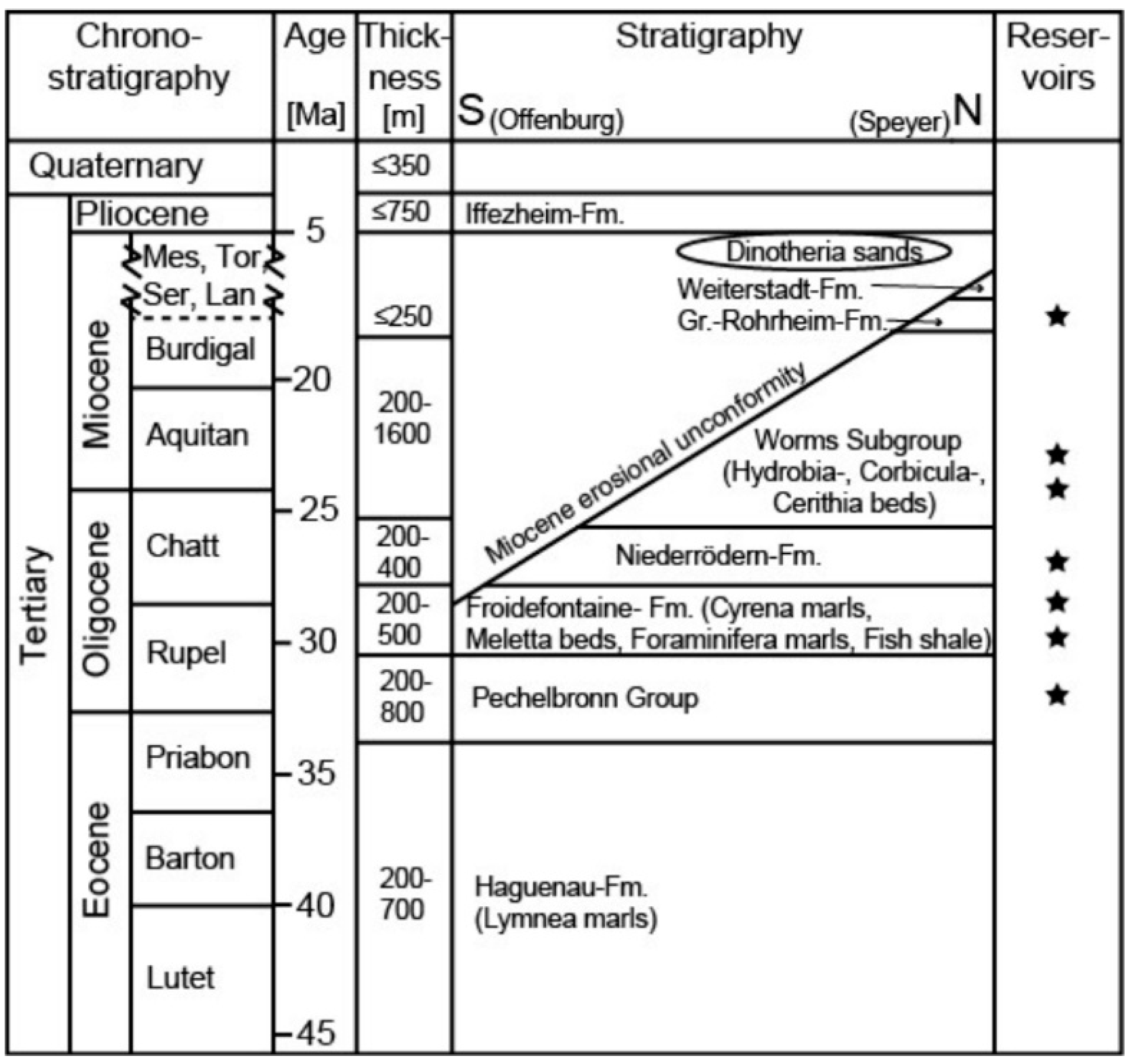
The Upper Rhine Graben (URG) is an about 300 km long NNE-SSW-trending continental rift system that has developed since about 47 Ma and accumulated up to 3.5 km of Cenozoic sediments (Figure 1). A first sedimentary sequence was deposited during WNW-ESE-extension at varying fluvial-lacustrine-brackish-marine conditions from late Eocene (c. 47 Ma) to Miocene (c. 16 Ma) times [41]. The deposition was followed by uplift and erosion mostly in the southern and central URG. This uplift and erosion phase caused a basin-wide unconformity in the URG, which can be identified in seismic sections [42]. Basin-wide deposition resumed in Pliocene times within the present NE-SW-transtensional stress field (Figure 1). For a review and further details of the geological development of the URG see [22] and references therein.
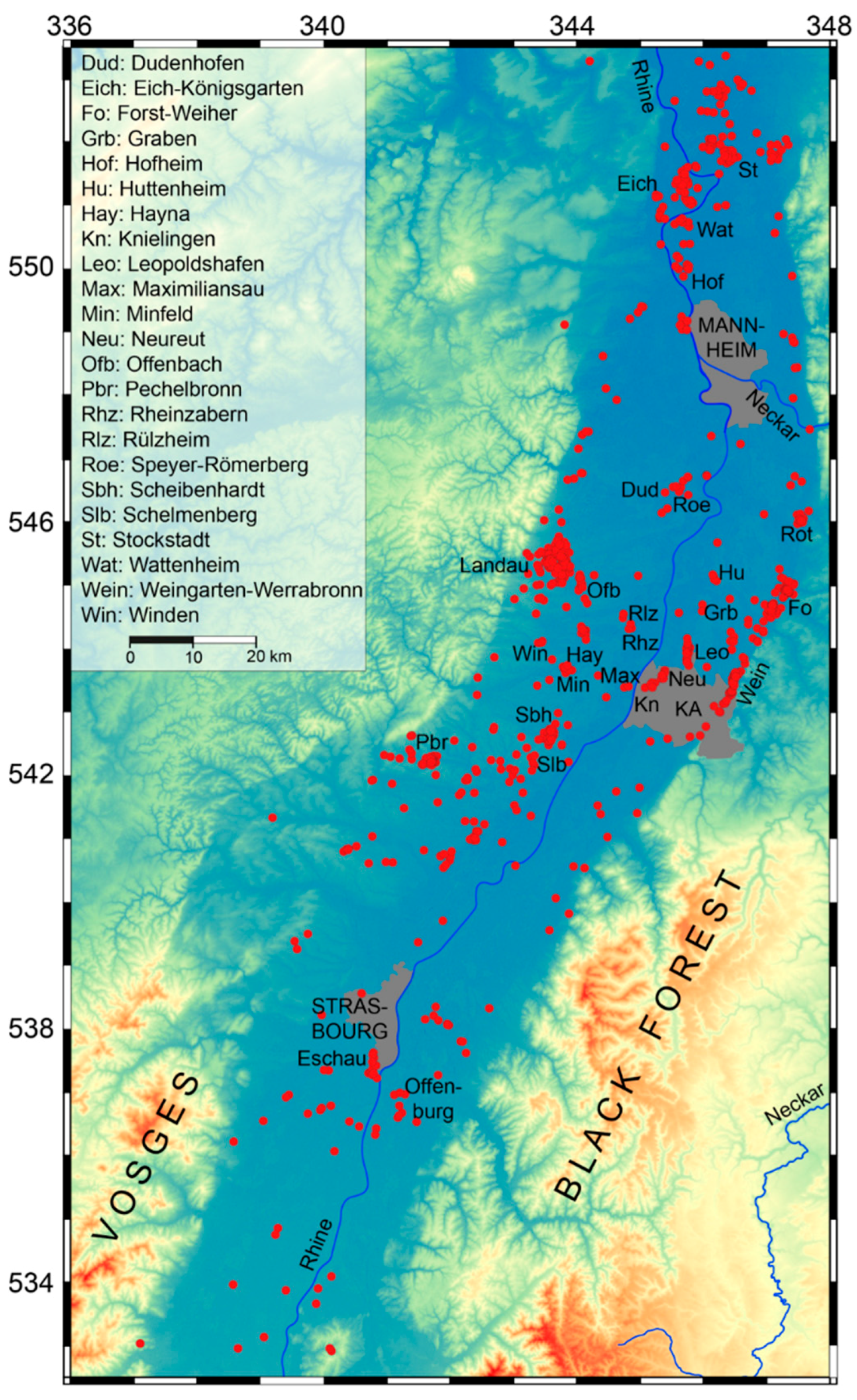
Hydrocarbon production in the URG occurred over more than 200 years, with a maximum of exploration and production activities in the 1950s to early 1960s (Figure 2; [43,44,45]). Modern research on the petroleum system, sedimentary-stratigraphic evolution, and diagenesis has been resumed in recent times [19,24,46,47,48,49].
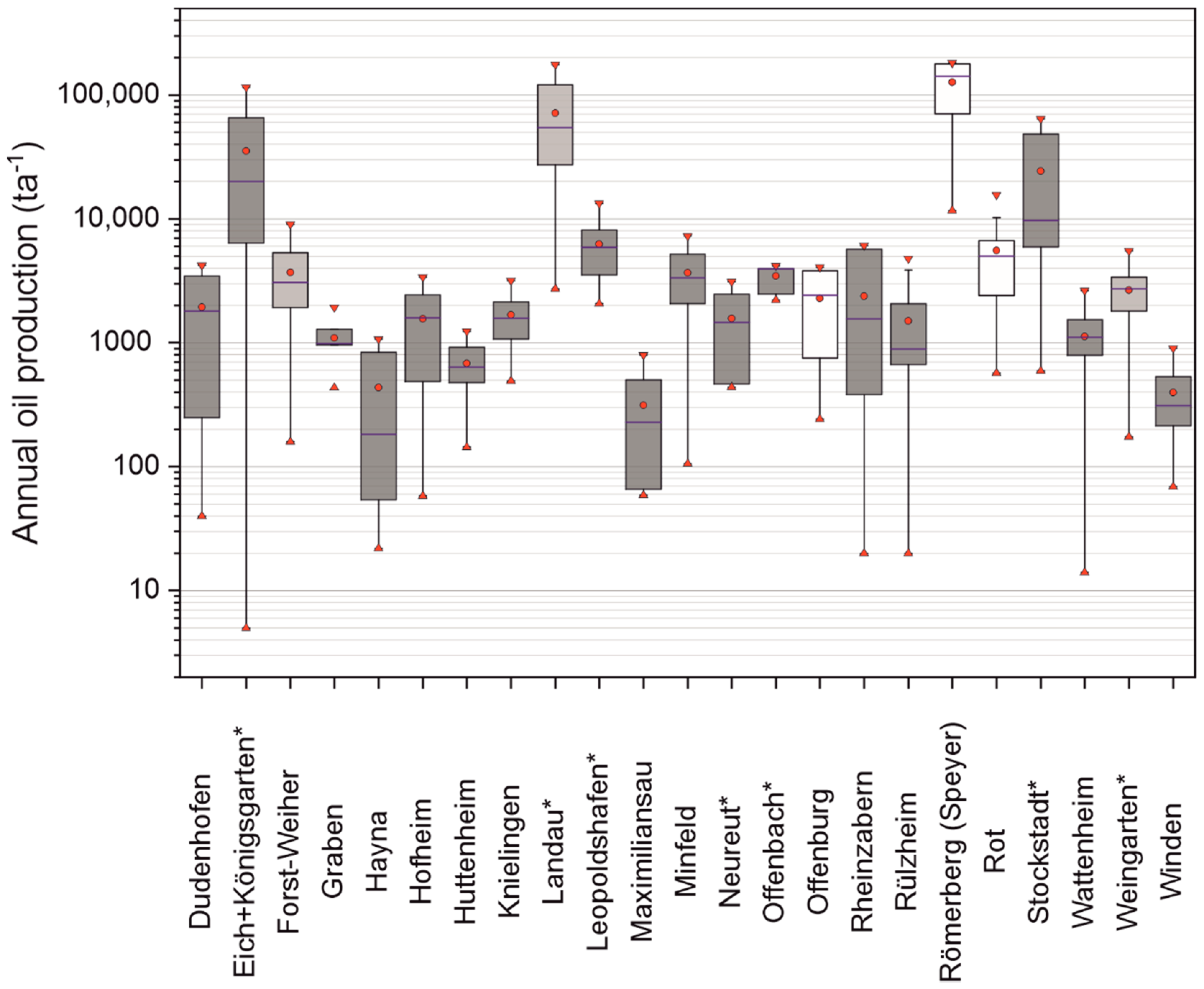
Oilfields in the URG can be either characterized by their origin from different source rocks (oil families A, B, C, D; [24]) or by their reservoir rocks from which the hydrocarbons have been extracted [45] and comprise either (i) Mesozoic rocks or (ii) both Mesozoic and Tertiary rocks or (iii) solely Tertiary rocks (Figure 3). Stacked reservoirs, i.e., production of oil from more than one reservoir either at the oilfield scale or at the borehole scale, are a characteristic feature in the URG for most oil fields. Figure 3 shows the range of the annual production of German oil reservoirs in the URG, which can be used to estimate their minimum storage capacities.
The permeability of Cenozoic reservoir rocks is predominantly porosity-controlled. These reservoirs occur mainly in (1) the Pechelbronn Group (Eich-Königsgarten, Stockstadt, Landau, Pechelbronn; [45]), (2) the Froidefontaine Formation, including the Meletta beds and Cyrena marls (e.g., Leopoldshafen), as well as (3) the Niederrödern Formation (e.g., Leopoldshafen, Knielingen, Hayna, Rheinzabern, Graben, Huttenheim) (Figure 3). Higher up in the stratigraphy, minor reservoirs of a few meter thick fractured dolomites and limestones rocks appear in the Worms Subgroup comprising the Cerithia, Corbicula, and Hydrobia beds. Medium to coarse-grained, weakly compacted sand layers in the Gr. Rohrheim and Weiterstadt Formations provide reservoir conditions for natural gas in the northern URG (e.g., Eich-Königsgarten; Stockstadt). These data typically originate from the boreholes drilled into the Tertiary stratigraphy. At the end of oil production at both individual borehole- and oilfield-scale the residual oil saturation, ROS, has commonly decreased to <10% [52,53]. In addition to low ROS, technical and economic reasons may also cause production stops. For locations at a larger distance from the oil-bearing parts of the reservoir, i.e., beneath the oil-water-contact (OWC), the reservoir rocks are assumed to be filled with formation waters with a negligible ROS; the reservoirs are thus referred to here as “depleted”. As hydrocarbons accumulate in the uppermost parts of a reservoir rock, the exploited oil commonly represents only a minor portion of the total volume of the reservoir rocks.
While the clay-rich Haguenau Formation essentially lacks significant reservoir rocks—except for few occurrences along the URG margins, the sequences of the Pechelbronn Group host reservoirs mainly in the northern URG (e.g., Eich-Königsgarten), but also along the eastern and western URG margins (Pechelbronn, Landau; [45]). The major Rupelian transgression caused full marine conditions in the URG and deposition of the Rupel Clay, a major basin-wide seismic reflector in the URG [42], representing the lower part of the Froidefontaine Formation [19]. Deposition of commonly 5–15 m, locally up to 23 m, thick calcareous fine-grained sand layers in the marine upper Meletta beds indicates short regressive phases [48]. The stratigraphically overlaying Cyrena marls, deposited under brackish conditions, host fine to medium-grained calcareous sand-rich channel fillings with typical thicknesses of <10 m, but locally up to >40 m [23,54]. These channel fillings pinch out within short lateral distances [54]. The Niederrödern Formation hosts ≤20 m, locally up to >30 m, thick fluvial and lacustrine fine-grained marly sand layers and lenses that show lateral thinning or pinch-out within several hundred meters [23,54]. Due to varying displacements between graben internal blocks [22,55], the depth of these reservoir rocks varies between the surface to about 2000 m [19,23,24,54,56,57] depending on their position between central and marginal fault blocks [22,55].
Due to the intense deformation of the sedimentary successions in the URG, structural hydrocarbon traps prevail over sedimentary traps [45,58]: Most hydrocarbons were trapped in slightly tilted sand-rich layers or lenses in the footwall of normal faults. These faults comprise either single (Leopoldshafen; [55]) or multiple structural traps that are structurally rather simple (Stockstadt, Eich, Scheibenhard; [59,60]) or more complex (Landau; [61]). Along the eastern URG margin dome structures comprise structural traps (Weingarten; [55]). Oil traps in gentle rollover structures occur locally (Knielingen, Neureuth; [55]). Unconformities are of particular importance in the northern URG (Eich; [60]) for natural gas trapped in sand-rich layers of the Groß Rohrheim- and Weiterstadt-Formations beneath the regional Miocene unconformity and for the Mesozoic reservoirs (e.g., Eschau, Römerberg (Speyer)) beneath the basal Eocene unconformity of the URG, commonly covered by sealing mudstones of the Haguenau Formation. In the southern parts of the URG, Eocene evaporites comprise important seals of Mesozoic reservoirs [59]. Hydrocarbon migration and accumulation appear to be a relatively young, possibly ongoing process in the URG that probably has been initiated during the late Miocene—early Pliocene times [45].
2.2. Thermal and Petrophysical Data of Reservoir Rocks
The URG is characterized by deep-reaching thermal anomalies resulting from fault-controlled convective fluid flow mostly within the crystalline basement and Mesozoic successions beneath low permeable clay-rich graben filling sediments [39,63]. These anomalies are also evident in the Cenozoic graben filling sediments, with temperatures locally exceeding 140 °C in 2 km depth [17,64] and geothermal gradients between 35 K km−1 and 58 K km−1, locally even reaching gradients of up to 100 K km−1 [50,54].
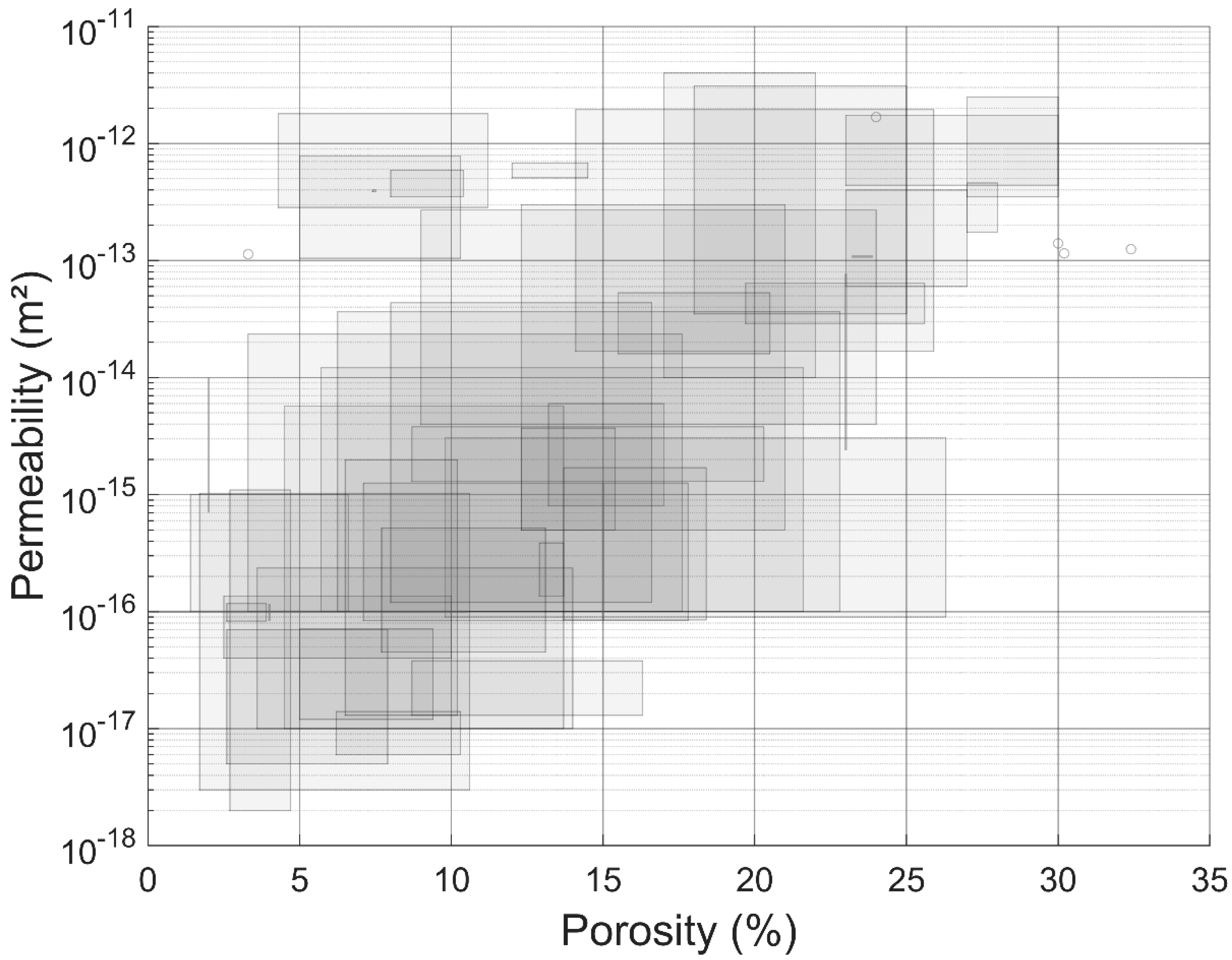
For heat storage systems, the hydraulic properties (e.g., porosity and permeability) of the rock are of key importance. Typical porosities and permeabilities of 5–20% and 10−16–10−14 m², respectively, are obtained from 85 core samples belonging to 39 exploration and production wells in 19 different oil-bearing Tertiary reservoir rocks in the URG [19,23,24,54,56,57]. Heterogeneous carbonate cementation and secondary carbonate dissolution [24] lead to porosities of 30% and permeabilities of 10−12 m² (Figure 4). While an exponential correlation between porosity and permeability is observed, both values show no straightforward correlation with depth and cannot be used to distinguish between different target formations. Note that due to larger uncertainties, logging data (as compiled by e.g., [65]) are not included in Figure 4 and not further considered.
Thermal properties of Tertiary rocks in the URG are very scarce and reveal large variations and uncertainties. Whereas thermal conductivities were measured on core samples [57,66,67], data on heat capacities are only available for comparable lithologies of the same age in the Northern German Basin [68,69].
3. Numerical Modeling
Data of depleted HC reservoirs in the URG are the basis of a numerical evaluation of the viability and efficiency of seasonal HT-ATES in these reservoirs. The numerical study is especially advantageous to quantify the impacts of uncertainties in the compiled geological and petrophysical data. Our modeling approach is limited to the REV concept (“representative elementary volume”; [70]) and the mutual coupling of hydrothermal processes. The modeling concept of the seasonal HT-ATES is assuming a doublet borehole system consisting of a cold and a hot leg with semi-annual injection and production load-time-functions (Figure 5). In this way, the cold leg is used for the injection during winter and the production during summer, whereas the hot leg is operated in the opposite configuration. It offers the advantage of installing specific temperature-dependent compounds in each well. Due to the low thermal diffusivities of rock [71] steady-state conditions cannot be reached after a foreseeable period. Therefore, a transient approach is used for modeling with a total simulation period of ten years.
3.1. Modeling Approach
The mass transport equation used to estimate the pore pressure, p, is given by mass balance along with the Darcy velocity, , as follows [70]:
is the mixture specific storage coefficient of the medium; t is the time; is the source/sink term for injection and production, is the permeability tensor, and are the fluid dynamic viscosity and density, respectively and is the gravitational acceleration. In the considered scale of geothermal storage, fluid dynamic viscosity, and density nonlinearly depend on temperature and pressure [72]. This nonlinearity leads to high computational efforts.
It is assumed that the solid and liquid phases in porous media are in local thermodynamic equilibrium. Heat transport, used to estimate the temperature, can be mathematically expressed using the advection-diffusion equation as:
and are the heat capacity and thermal conductivity of the mixture, respectively. represents the heat capacity of the fluid. The open-source code TIGER (THC sImulator for GEoscientific Research; [73]) has been deployed, which is based on the described assumptions and implemented within the object-oriented framework MOOSE [74,75].
With ROS being ignored for the simulated water-bearing formations, only single-phase flow is considered. It is assumed that injection and production take place below the oil-water contact in the reservoir layer and are not affected by accumulations of residual oil. Besides, it may be assumed that potential ROS is further reduced after a few injection and production cycles having washed out any oil traces.
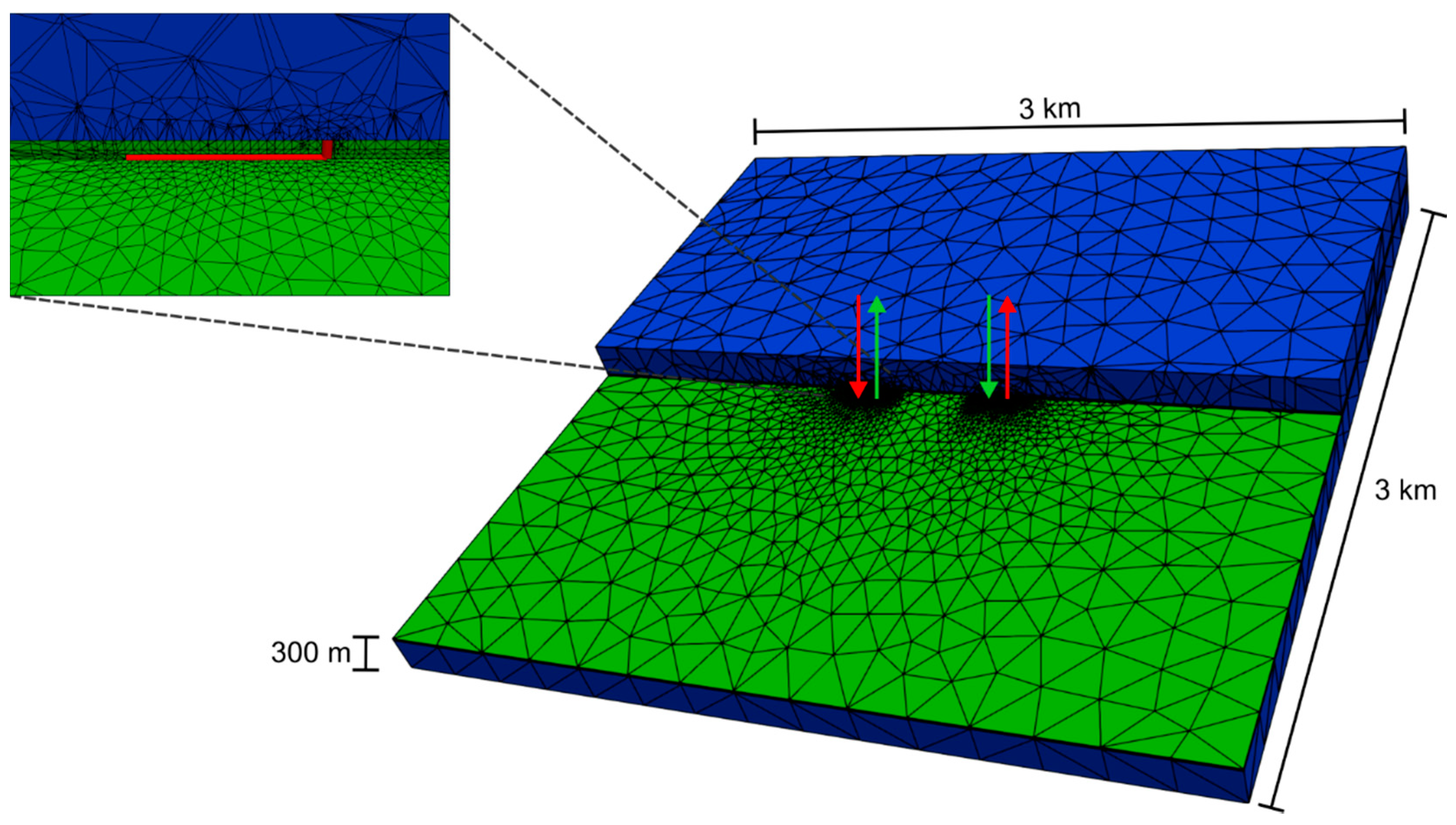
A generic 3D model of a potential HT-ATES site in the URG represents the core of the numerical study. The center of the reservoir is assumed to be at a depth of 1.2 km corresponding to an average value of former oil reservoirs. The lateral extension of the model (3 km × 3 km) is chosen to avoid any boundary effects on the area of interest. Vertically, the model extends over 300 m with three layers assumed: the reservoir in the center of the model with variable thicknesses of 5, 10, or 20 m and two confining layers with equal thicknesses (Figure 5). The selected thickness values of the confining layers further assure that top and bottom boundaries do not affect the modeling area of interest. Two wells are located in the center of the model with a lateral distance of 500 m from each other to avoid any thermal interference between the wells as this significantly reduces the storage efficiency [73,76]. Two different well trajectories were considered: (1) vertical boreholes only and (2) a vertical section covering the top half of the reservoir layer with a horizontal section of 100 m length in the center of the reservoir layer pointing in opposite directions. While the vertical design represents a normal borehole, the addition of a horizontal section represents a technical approach to increase the contact area between the borehole and the reservoir, similar to the effect of a larger reservoir thickness.
The unstructured mesh consisting of tetrahedral elements was created by the Gmsh software [77]. The element sizes vary between 2.5 m (along the vertical well sections) and 187.5 m (at the model boundaries). Further refinement was performed along the horizontal well sections as well as in the area surrounding the wells where the highest gradients of the pressure and temperature field are expected to occur. A mesh sensitivity analysis was performed to avoid any mesh dependency on the results. In total, the model contains 18,589 nodes connected by 107,894 elements.
Hydrostatic pore pressure was applied to the model by setting Dirichlet boundary conditions (BCs) at the top and the bottom of the model domain with an associated initial condition (IC). Injection and production flow were implemented by using time-dependent mass flux functions at the top of the reservoir with six months’ cycles. These time-dependent functions represent simplified approximations of a real pumping operation by assumed instantaneous reversal of the pumping direction at the end of each cycle. The temperature distribution within the model is based on a favorable geothermal gradient of 50 K km−1 under the URG setting (see above). It was achieved by setting Dirichlet BCs at the top and the bottom of the model domain and corresponding ICs throughout the model. To implement the injection of water with a specific temperature into the two wells, Dirichlet BCs at the top of the reservoir (corresponding to the beginning of the open hole section) are activated during the injection period of the respective well.
It is considered that the hydraulic operational parameters imply major constraints for the operation of HT-ATES. Both, flow rate and associated pressure changes involve a potential hazard to induce micro-earthquakes. Herein, we assume a cautious operation in an urban or sensitive environment limiting the hydraulic parameters to a maximum overpressure of Pmax = 2 MPa and flow rate of Qmax = 10 Ls−1. Experience has shown, that this Pmax/Qmax combination does not create a major mechanical impact (induced seismicity; [78,79]) on a reservoir. This cautious combination can be exceeded under specific conditions. Model simulations are thus aborted if pressure changes caused by the injection exceed this Pmax threshold.
3.2. Reference Case
A reference model (hereafter called “reference case”) of typical parameterization (Table 1) was developed to demonstrate the general behavior of an HT-ATES. It also serves for comparison to further parameter sensitivity studies. The two seasonal operation modes are represented by injection with a temperature of 140 °C in the hot well during the summer (using the cold well as producer) and an inverted mode during the winter when water with a temperature of 70 °C (i.e., the ambient reservoir temperature) is injected in the cold well (using the hot well as producer).
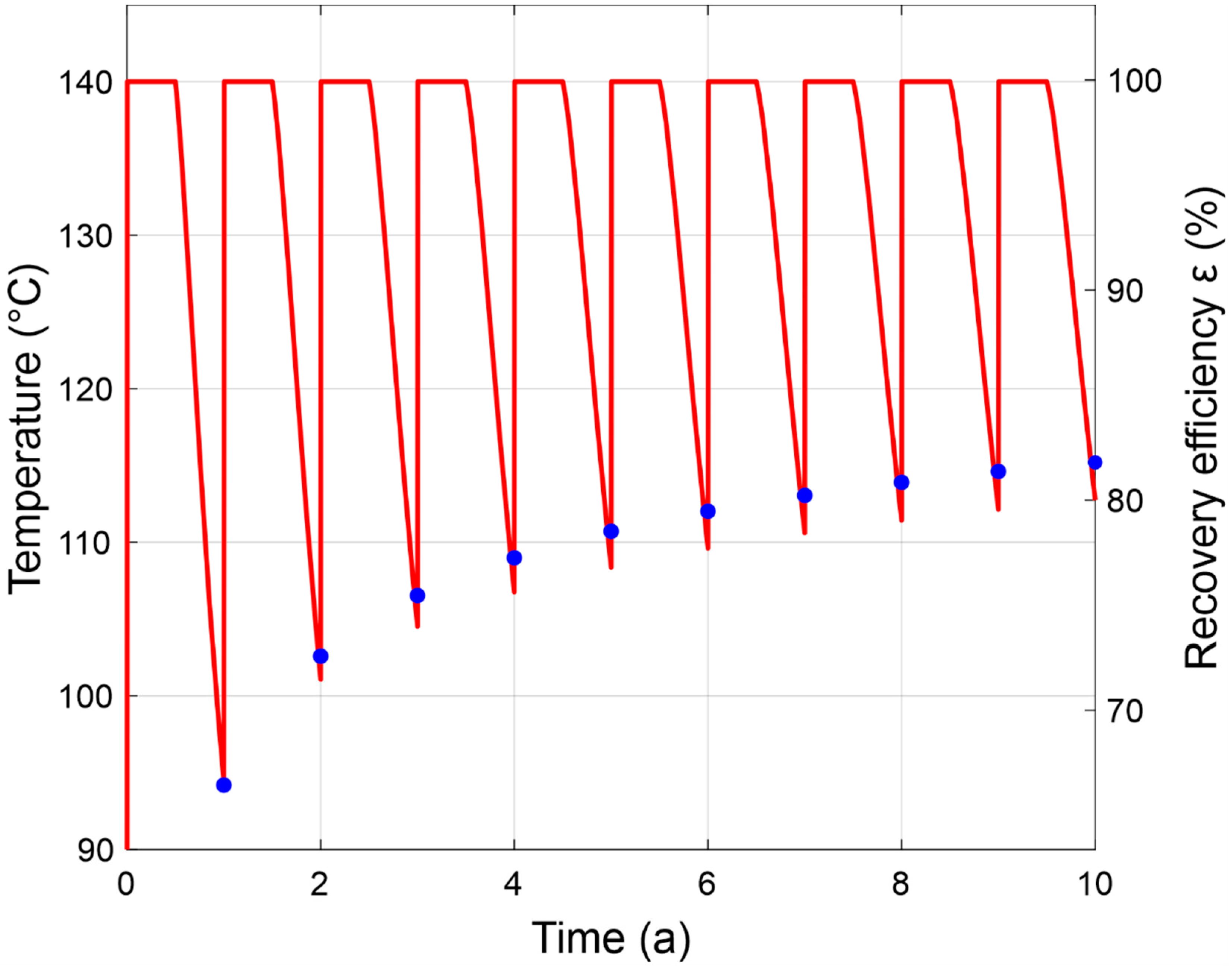
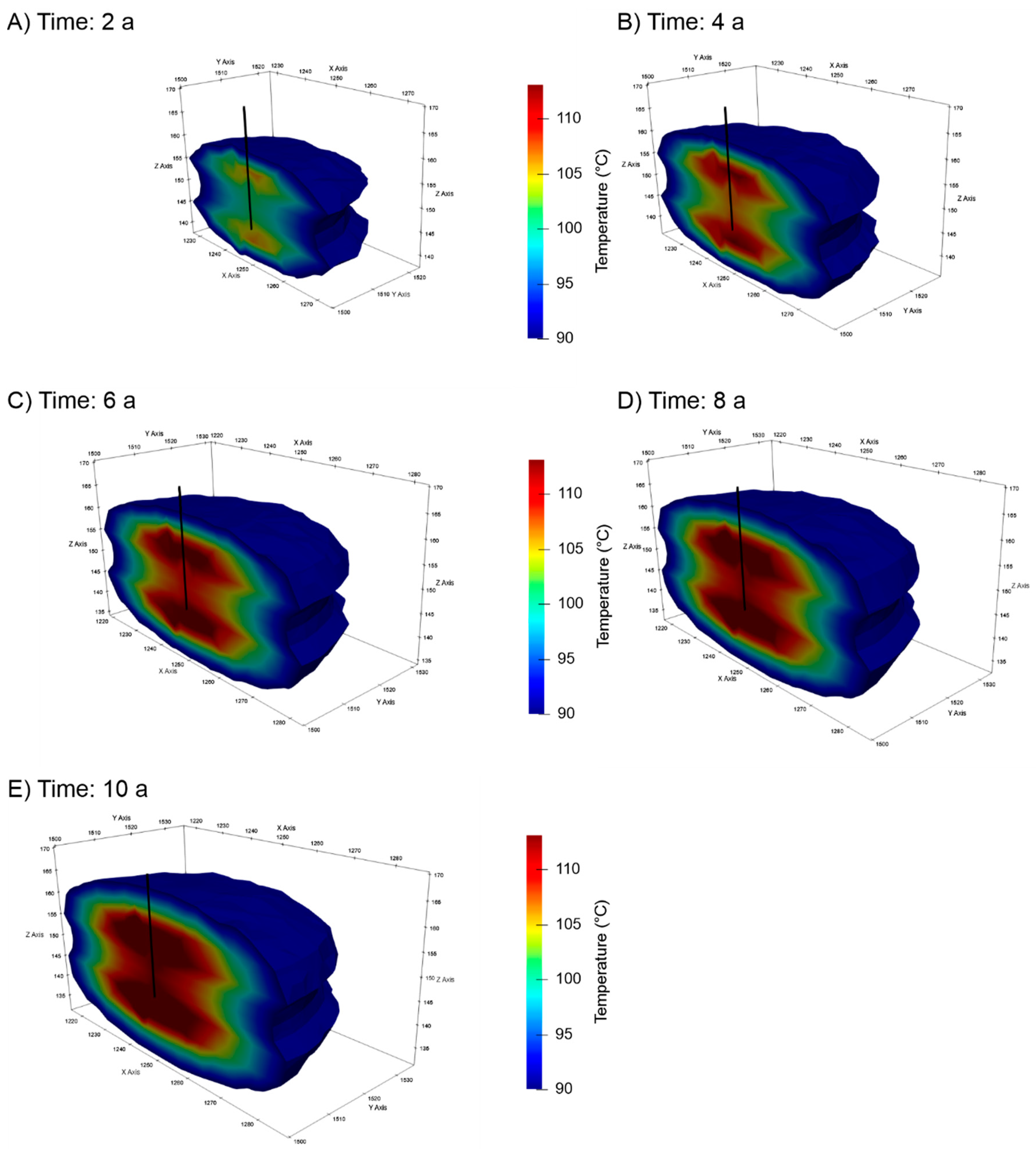
The selected temperature conditions do not imply an energy balanced storage operation. The setting involves a negative energy budget due to the diffusive losses around the hot well as water with a temperature exceeding the ambient reservoir temperature is stored. As a result, the simulation is resulting in continuous warming of the reservoir next to the hot well. The minimum production temperature at the end of each winter operation increases from 94.5 °C after the first year to 112.7 °C after the 10th year (Figure 6). It reflects the accumulation of thermal energy in the reservoir that is also shown in Figure 7. This behavior agrees with earlier assessments of geothermal storage systems [35]. Under the assumed conditions the thermal perturbation during injection extends over a maximum distance of 90 m from the hot well after 10 years. The accumulation of heat leads to a slow temperature increase in the reservoir and yields a decreasing diffusive heat loss with time [32]. The temperature difference of 70 K between injection and ambient conditions will thus reduce with time and reservoir temperature asymptotically approaches injection temperatures of 140 °C at near steady-state conditions. This contrasts the behavior of shallow storage systems with smaller temperature differences close to a balanced energy budget [35], where near steady-state conditions are reached after a comparably short operation time of already three years.
This behavior is reflected by an improved recovery efficiency, ε. It represents an important parameter for the feasibility of heat storage systems and is defined as the ratio between extracted and stored energy. Since the conditions at the cold well do not change, ε characterizes the conditions at the hot well:
With Tp(t) the production temperature, Ti(t) the injection temperature, and Ta the average initial reservoir temperature. Herein, ε is calculated for periods with a length of one year.
Figure 6 shows an increase in ε from 66% in the 1st year to 82% in the 10th year. These values correspond to the amount of extracted energy increasing from 1.8 GWh to 2.2 GWh under the conditions of the reference case with 2.7 GWh of heat injected annually in the reservoir. These high ε values seem to be representative for geothermal systems as they confirm earlier studies for low [35] or high-temperature storage [31,82]. The increase of ε of 16% in the reference case compares well to earlier studies on shallow thermal storage, implicating increases between 1% and 30% [30,32].
4. Parameter Sensitivity on Recovery Efficiency
The findings of the reference case exemplify the behavior of an HT-ATES based on an average reservoir parametrization of the URG. Chapters 2.1 and 2.2 show a large variety of relevant parameters for a general resource estimation of depleted hydrocarbon reservoirs in the URG. Herein, we systematically investigate the influence of the most important reservoir parameters and the drilling trajectory to determine their impact on storage efficiency, using an adapted and extended filtering concept, which was originally developed in Gholami Korzani et al. [73]. The following sensitivity range is investigated (Table 2):
4.1. Parameter Variation for the Vertical Well Setup
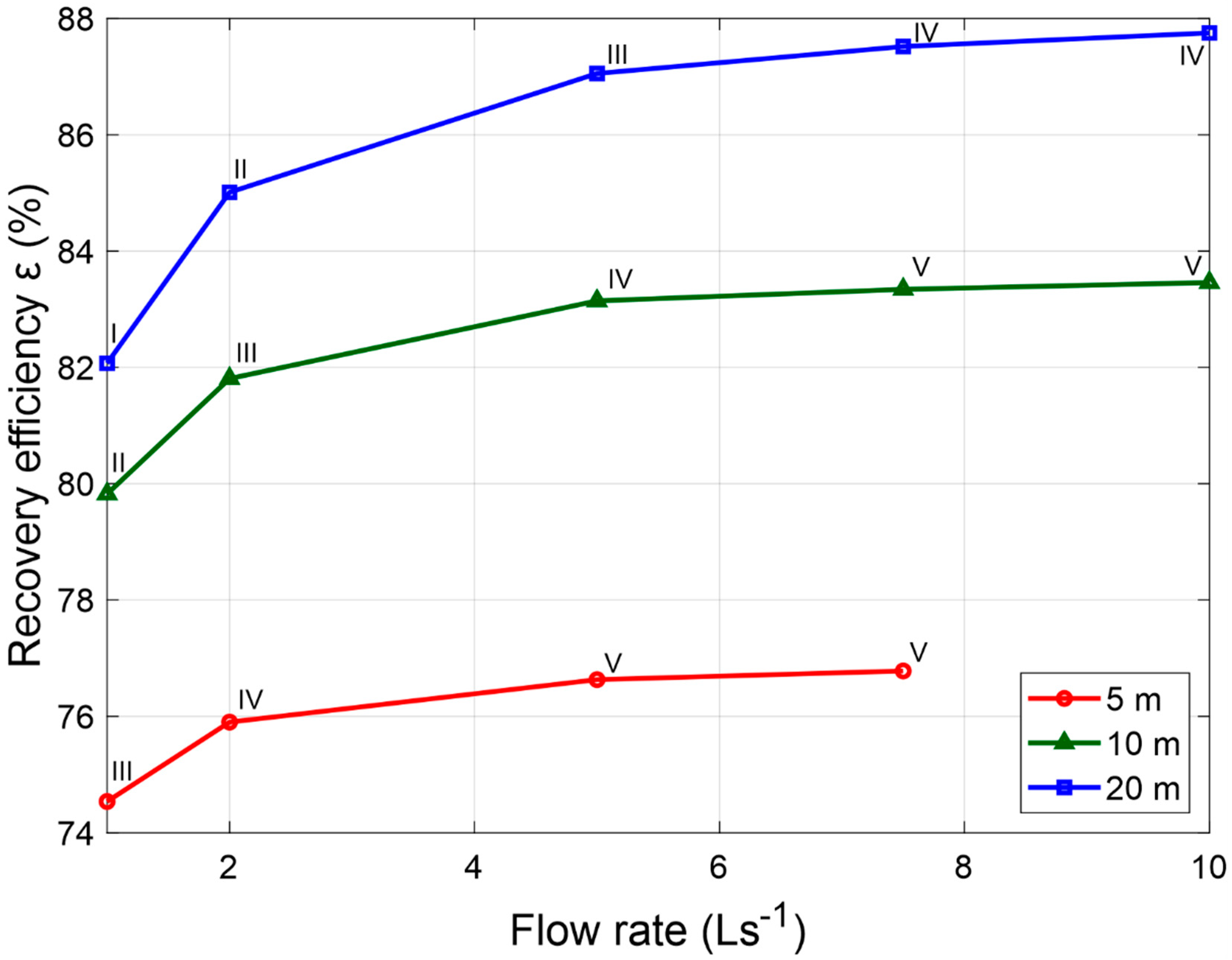
The influence of reservoir thickness, permeability, and flow rates on ε is first investigated with constant thermal conductivities (λres = 2.5/λcap= 1.4 Wm−1K−1) for a vertical well setup. For the parameter variation an adapted grid sampling was used based on Table 2 (see Table A1). Figure 8 shows the impact of reservoir thickness and flow rate on ε with higher values being obtained for higher thicknesses and flow rates. After the 10th operation cycle is reached for a thickness of 5 m and ε of up to >87% for a thickness of 20 m. Under the constraints of the Pmax threshold, typically a minimum permeability between 10−14 m² and 10−13 m² (cases I and IV in Figure 8) is required for these HT-ATES with even higher values for higher flow rates. At a given permeability, high reservoir thicknesses allow for more variable flow rates due to their lower injection pressure, e.g., at 10−13 m² flow rates can increase up to the Qmax = 10 Ls−1 threshold, whereas at 10−14 m² flow rates can only reach 1 Ls−1.
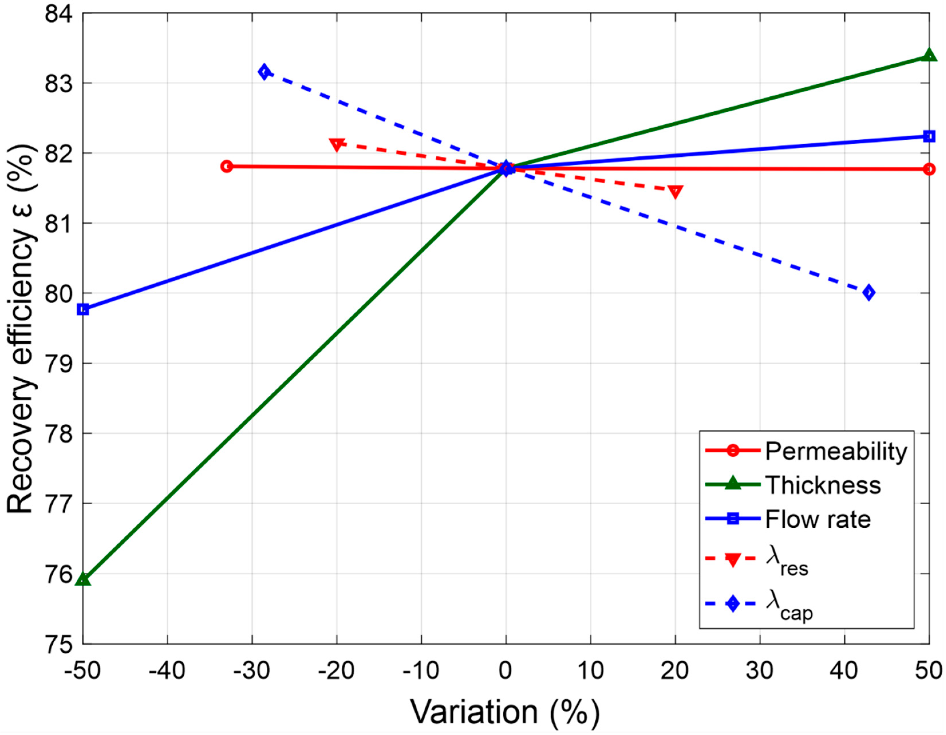
The sensitivity of these three parameters on ε is illustrated in Figure 9. Due to the limitations set by the Pmax threshold, the sensitivity was calculated in comparison to a model slightly different from the reference case (with a permeability of 10−13 m² instead of 6.6 × 10⁻¹⁴ m²). A variation of reservoir thickness represents the strongest individual influence on ε with a 50% variation leading to a change in ε of nearly 10%. The same variation for flow rate leads only to a change in ε of 2%. Although reservoir permeability shows only a low influence on ε, its importance arises from its impact on the pressure evolution in the reservoir and thus the operation with high flow rates. It can be concluded that major attention should be paid to the reservoir thickness when choosing a potential HT-ATES site.
Figure 9 also illustrates the influence of thermal conductivity. For this purpose, the flow rate was kept constant at 2 Ls−1 and reservoir permeability at 10−13 m². The importance of proper treatment of λres and λcap is highlighted by the fact that the impact of their variation on ε reaches the same order of magnitude as changes in flow rate and reservoir thickness. This means that variations of thermal conductivities in the subsurface should receive equal attention as hydraulic and geometrical reservoir parameters in the planning of HT-ATES sites. On the other hand, this further implies that all results regarding the variation of hydraulic and geometrical parameters are additionally subjected to the described uncertainties related to varying thermal conductivities of both the caprock and the reservoir.
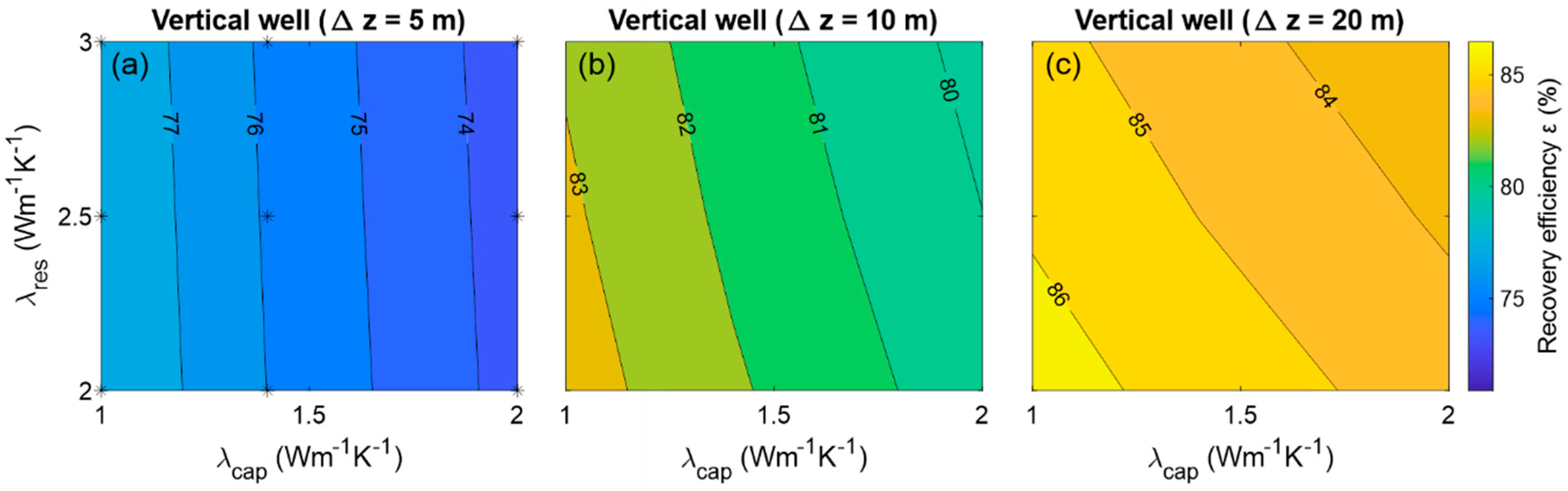
Figure 10 provides more details to this statement for variations of λres and λcap. Typically, a lower λcap tends to isolate the reservoir leading to higher ε whereas higher values imply higher heat losses. At lower reservoir thicknesses a variation of λres is nearly insignificant (manifesting as vertical ε isolines in Figure 10a). λres is only getting important when the reservoir thickness increases drastically, yielding inclined ε isolines (Figure 10c). This effect is caused by the decreasing influence of the caprock (acting as a thermal insulator) on the propagation of the injected hot water.
4.2. Comparison of Vertical and Horizontal Well Setups
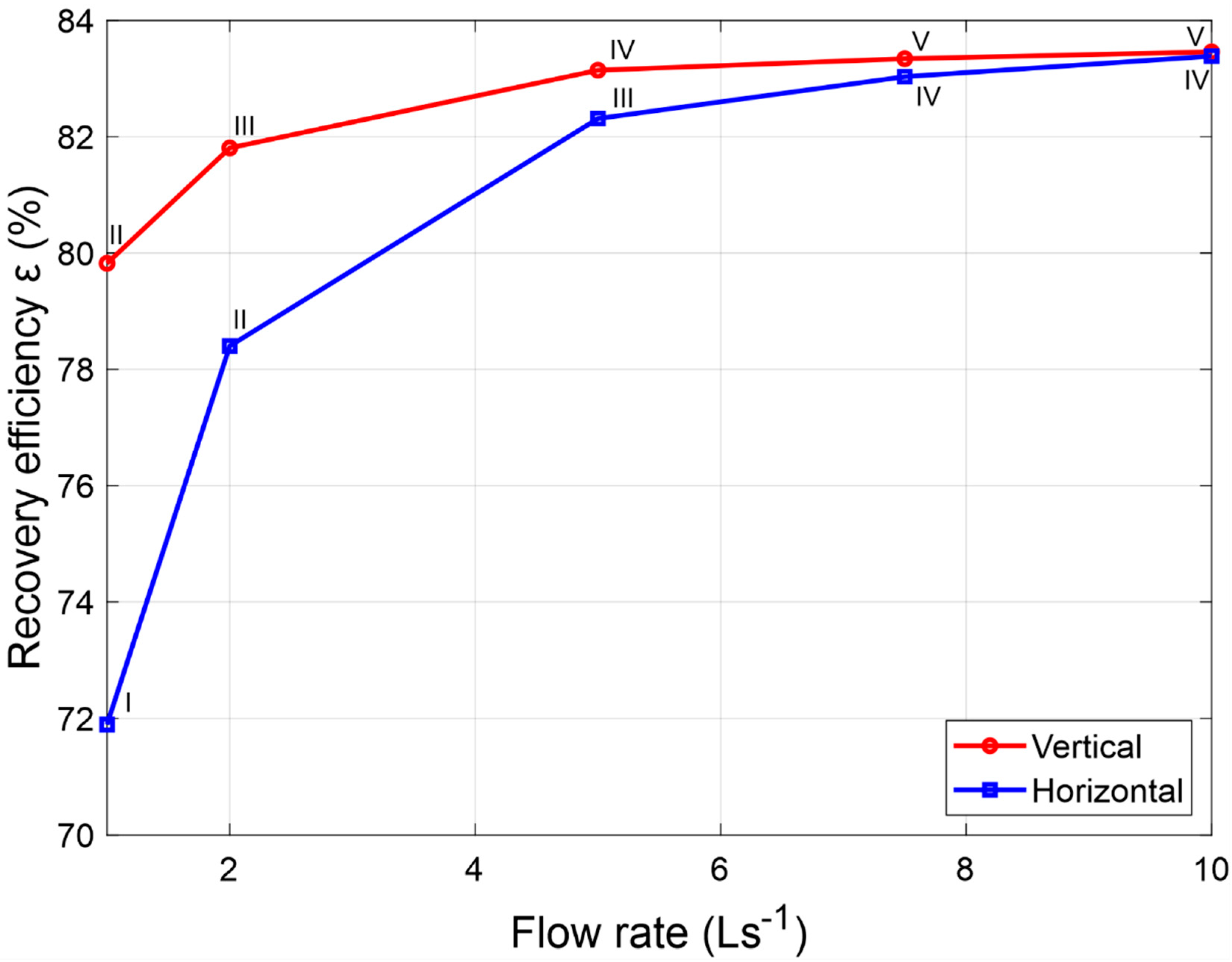
Drilling horizontal wells are becoming a standard procedure for the exploitation of hydrocarbon reservoirs [83,84] and could also be a possible blueprint for geothermal storage. Therefore, and particularly concerning the geological setting of potential reservoir layers in the URG, the influence of the well setup on the operation of HT-ATES is investigated by comparing the vertical well setup with a 100 m long horizontal well setup. Figure 11 shows the results for a 10 m thick reservoir layer with permeability and flow rate variations as provided in Table 2.
The horizontal well section leads to reducing pressure variations within the reservoir due to the larger contact area between the well and the reservoir compared to the vertical drill path. Consequently, higher operational flexibility could result from applying higher flow rates or utilizing reservoirs of otherwise uneconomically low permeability (Figure 11). For a permeability of 10−13 m² (case IV in Figure 11), for instance, drilling of such a horizontal well section leads to an increase of the maximum flow rate from 5 Ls−1 to 10 Ls−1 or reservoirs with a permeability of 10−14 m² (case I in Figure 11) could still be used. However, drilling horizontal wells could also have minor adverse effects. At low flow rates, the higher heat transfer through the larger surrounding surface area will increase heat losses and results therewith in lower ε. This difference diminishes with higher flow rates.
5. Discussion and Possible Energy Extraction in the URG
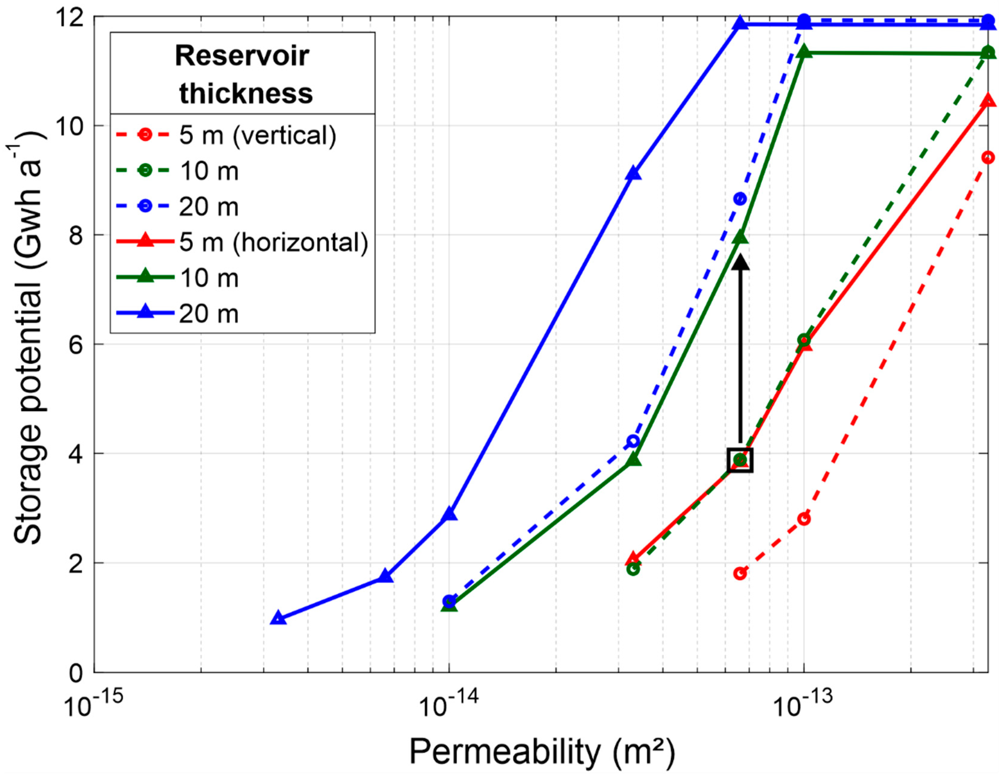
To assess the potential of specific HT-ATES systems, it is necessary to consider the storage capacity, i.e., the total energy stored and extracted, rather than recovery efficiencies. Herein, we refer to the storage capacity ΔEstor as the total amount of energy extracted during the 10th year of operation. Figure 12 compares ΔEstor for the vertical and the horizontal well setup for identical Pmax constraints (i.e., all models assume P = Pmax at injection). It can be observed that ΔEstor varies between values of 1–12 GWh a−1 and increases with reservoir permeability and thickness. Despite slightly lower recovery efficiencies, the use of the horizontal well setup leads to a significantly higher absolute storage capacity for the given permeability/thickness combination due to higher total flow rates. Especially in the critical permeability range between 10−14 m²–10−13 m², the horizontal well setup offers advantageous settings. The results of Figure 12 are further constrained by the Qmax threshold limiting the maximum storage capacity of the power plant. Thus, the maximum capacity can become independent of the borehole geometry if the maximum flow rate is reached resulting in a maximum storage capacity of 12 GWh a−1. At a higher Qmax threshold, the storage capacity could further increase.
The possible gain in ΔEstor through horizontal wells is illustrated by comparing the reference case (vertical well, black square in Figure 12) to its horizontal counterpart (black arrow in Figure 12). Under the given threshold conditions, the reference case allows the storage of 3.9 GWha−1, whereas a horizontal well reaches 7.9 GWha−1. This corresponds to an increase of about 100% in annual storage capacity.
The described higher storage capacity of the horizontal well setup is mainly of importance at low permeability and/or low reservoir thickness since it can turn uneconomic exploitation into a valuable business case. For reservoirs with very low permeability (<10−14 m²) and thicknesses, longer horizontal well sections could thus be considered. For instance, a well with a 500 m long horizontal section would even allow the exploitation of reservoirs with permeability ≥10−15 m². However, since this also results in higher investment costs, the vertical well setup can be more economically viable for high permeabilities. The optimal well setup has always to be determined specifically for each potential site.
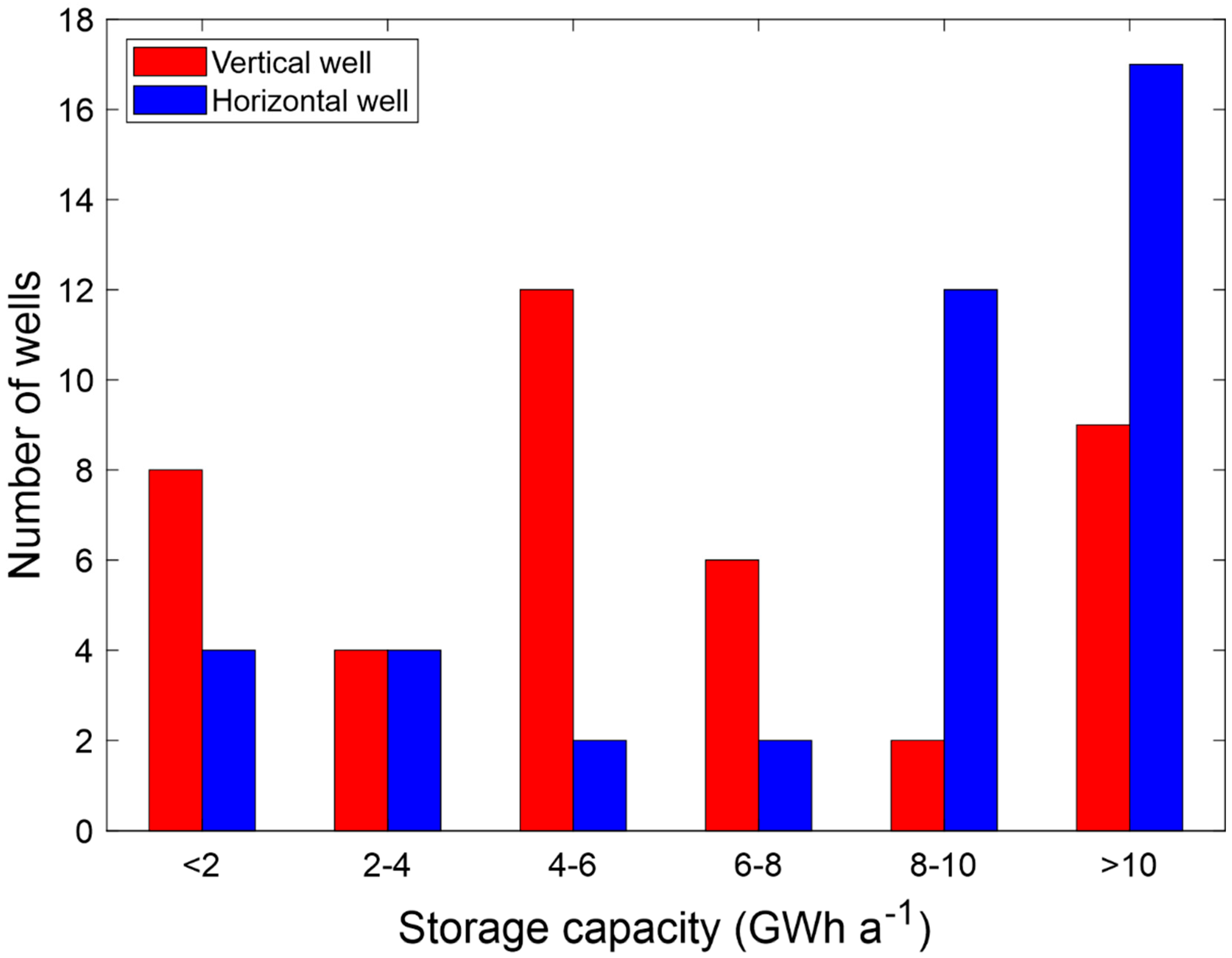
As the last step of this potential analysis, the assessment of ΔEstor of potential HT-ATES in depleted oil fields of the URG needs to be tackled. Herein, we combine our synthetic numerical findings with the available data from oil reservoirs. This evaluation is limited to a subset of reservoirs described in Chapter 2 with available measurements on permeability and thicknesses consisting of 41 wells in 10 reservoirs (as shown in Table A2). A histogram of possible storage capacity is provided in Figure 13 derived from the parameter range of this subset assuming a vertical/horizontal well setup and thermal conductivities of the reference case (λres = 2.5 and λcap= 1.4 Wm−1K−1) as only scarce information on λres and λcap in the URG exists. As expected, the storage capacity of the horizontal wells is more favorable compared to vertical wells. Figure 13 indicates a maximum ΔEstor for vertical wells between 4 and 6 GWh and for horizontal wells at ΔEstor > 10 GWh. This distribution is especially a clue for the realization of these systems with ΔEstor > 8 GWh being reached for approx. 70% of all horizontal wells but only 27% of the vertical wells.
Assuming a minimum economic threshold of ΔEstor = 2 GWh as reached, for example, by the Reichstag storage system in Berlin [85], 80% of the vertical and 90% of the horizontal wells would provide sufficient reservoir conditions. Even if the minima of the underlying data are considered as representative instead of average values, a considerable number of reservoirs would still meet the assumed economic threshold (46% of the vertical and 76% of the horizontal wells).
If we assume that the selected subset of reservoirs is representative of all depleted oil reservoirs, the total potential of HT-ATES in the URG can be estimated. In the URG, 26 German and 36 French depleted oil reservoirs exist (including reservoirs with exploration activity only) and characteristically constitute stacked reservoirs with more than one reservoir layer. The exploitation of these reservoirs by horizontal wells could lead to a storage potential in the magnitude of up to 1′000 GWh a−1 assuming average capacities of approx. 10 GWh a−1. The exploited area even of horizontal wells is typically restricted to a 100 m distance from the well (see example in Figure 7) leading to a storage area of less than 1 km² assuming a lateral distance of 500 m between the boreholes. Especially in the case of the laterally extensive Meletta beds, it may be assumed that the potentially usable size of the depleted reservoir exceeds this storage area, leading to a possible realization of multiple storage doublets per reservoir. This may further scale the potential capacities of HT-ATES in the URG to the magnitude of up to 10 TWh a−1. This order of magnitude compares well to the regional thermal energy demand. Taking as a basis the annual thermal energy need of Germany of 1800 TWh [86], the annual thermal energy need for the 6 million inhabitants in the URG [87] would scale down to 135 TWh. In this context, HT-ATES would cover a significant share in a sustainable manner. However, future analyses have to focus also on a life cycle analysis considering the intrinsic energy need for operating these systems and have to quantify the economic impact. Potentially available sources of sustainable heat may include excess heat from geothermal production (i.e., from deeper reservoirs such as the Mesozoic Buntsandstein) or solar energy as well as waste heat of industrial processes. However, numerical studies and economic analyses are of limited significance and cannot replace the analysis of real systems. Therefore, the potential of this new geothermal technology needs to be quantified by scientific demonstrators.
6. Conclusions and Outlook
HT-ATES could potentially play an important role in storage scenarios required for a climate-neutral society, but this new technology has to prove its feasibility and meet the necessary public acceptance. In this respect, areas of former hydrocarbon production could provide both, the necessary reservoir conditions and the knowledge on these as well as the local experience of low-hazard hydrocarbon production for more than 50 years. Based on the extensive production experience, it can be expected that the storage operation in the soft, clay-rich sediments of the Tertiary rock to be mostly aseismic. Moreover, a low flow rate—much lower than required for geothermal power production—is applicable, further reducing the seismic risk, especially for densely populated areas.
Such a concept could also perfectly symbolize the transition from a hydrocarbon-based past to renewable energy in the future. As shown by this study, depleted oil reservoirs represent an important resource potential for HT-ATES systems in the URG. Despite the modest permeability and thickness of the investigated reservoirs, they could mostly (i.e., about 80% of all investigated sites) be used for HT-ATES with storage capacity, ΔEstor above 2 GWh. Other promising sandstone layers and lenses occur in the Cenozoic successions of the URG, known from exploration drillings, that lack accumulation of hydrocarbons and therefore largely escaped detailed petrophysical investigations. Some of these sandstones most likely accumulated hydrocarbons in the past, but these previously accumulated hydrocarbons were probably ‘flushed’ away due to tectonic activities [55].
The presented study could benefit from the large database of the abandoned oil reservoirs in the URG, comprising detailed petrophysical and stratigraphic information. However, the data from the hydrocarbon exploration and operation can partly not simply be transferred into a hydraulic-driven thermal storage system and seem to be most reliable for core measurements of the ambient rock. Future analyses should investigate (1) the impact of residual oil concentration in the reservoir on HT-ATES operation and efficiency, as well as (2) the influence of chemical reactions in the reservoir, e.g., dissolution/precipitation of mineral phases due to the injection of hot water and their influence on porosity/permeability. It is noteworthy to mention the applied simplifications concerning constant reservoir parameters and horizontal geometries, whereas our data compilation exhibits significant heterogeneities due to complex geological processes [54]. Herein, we quantified this impact in our sensitivity analysis, however, future applications have to investigate this effect further.
The results show that the storage capacity of HT-ATES in depleted oil reservoirs of the URG depends most sensitively on reservoir thickness, the applied injection/production flow rates, and the thermal conductivities of the reservoir caprock. The results identify the high recovery efficiency in HT-ATES in depleted oil reservoirs reaching values of >80%. Assuming the above-considered injection temperature, deeper, thus warmer, reservoirs would be even more efficient, and a further increase of the recovery factor by >5% can be expected. The numerical study demonstrated the benefit of operating a horizontal well orientation. Under these conditions, a considerable part of the reservoirs could be utilized in an economically viable manner. Not surprisingly, the deployment of advanced technologies such as directional drilling or geosteering promises optimum success. The order of magnitude of the estimated annual storage capacities of depleted oil reservoirs in the URG of up to 10 TWh represents a significant part of the thermal energy demand of the population in the URG. Furthermore, as numerical studies cannot replace the analysis of real systems, scientific demonstrators are needed for a proof of concept. For future economic use, further studies including life cycle analyses are essential.
Author Contributions
Conceptualization, K.S., E.S. and T.K.; methodology, K.S., J.C.G., R.E. and M.G.K.; software, M.G.K.; formal analysis, K.S.; investigation, K.S., J.C.G.; data curation, K.S.; writing—original draft preparation, K.S., J.C.G.; writing—review and editing, R.E., J.B., M.G.K., E.S., T.K.; visualization, K.S., J.C.G.; supervision, T.K., E.S. All authors have read and agreed to the published version of the manuscript.
Funding
Eva Schill acknowledges funding through the Helmholtz Climate Initiative (HI-CAM) which is funded by the Helmholtz Association’s Initiative and Networking Fund. The authors are responsible for the content of this publication.
Acknowledgments
We thank Ali Dashti (Karlsruhe Institute of Technology) and Jörg Meixner (Baden-Württemberg State Authority for Geology, Mineral Resources, and Mining) for their contributions in the early stages of this study as well as Katharina Schätzler (Karlsruhe Institute of Technology) for her assistance in the DeepStor project. The support from the Helmholtz program “Renewable Energies” under the topic “Geothermal Energy Systems” is thankfully acknowledged. The Helmholtz Climate Initiative (HI-CAM) is funded by the Helmholtz Association’s Initiative and Networking Fund. The authors are responsible for the content of this publication. We further thank the EnBW Energie Baden-Württemberg AG for supporting geothermal research at KIT.
Conflicts of Interest
The authors declare no conflict of interest.
Appendix A

Table A1.
Parameter variation used for the parameter sensitivity analysis on recovery efficiency.
| Parameter | Variation | ||||||||
|---|---|---|---|---|---|---|---|---|---|
| Reservoir permeability [m²] | Vertical well | 6.6 × 10⁻¹⁵ | 1 × 10⁻¹⁴ | 3.3 × 10⁻¹⁴ | 6.6 × 10⁻¹⁴ | 1 × 10⁻¹³ | 3.3 × 10⁻¹³ | ||
| Horizontal well | 1 × 10⁻¹⁵ | 3.3 × 10⁻¹⁵ | 6.6 × 10⁻¹⁵ | 1 × 10⁻¹⁴ | 3.3 × 10⁻¹⁴ | 6.6 × 10⁻¹⁴ | 1 × 10⁻¹³ | 3.3 × 10⁻¹³ | |
| Reservoir thickness [m] | 5 | 10 | 20 | ||||||
| Thermal conductivity [Wm−1K−1] | Reservoir (λres) | 2 | 2.5 | 3 | |||||
| Cap rock (λcap) | 1 | 1.4 | 2 | ||||||
| Injection/production flow rate [Ls−1] | 1 | 2 | 5 | 7.5 | 10 | ||||
Table A2.
Overview of 41 wells from 10 depleted French and German oil fields in the URG that are used to assess their potential for HT-ATES in Chapter 5. The data also include values obtained from log calculations. The reservoir permeability (1 × 10⁻¹⁵–4 × 10⁻¹² m²) and thickness (3–48 m) distributions of these wells map representative values of the data basis in the Upper Rhine Graben (see Chapter 2). The abbreviations of the reservoir formations stand for the following: Niederrödern Fm. (NF), Cyrena marls (CyM), Meletta beds (Me), Pechelbronn Fm. (PBF), Eocene basis sands (EBS), Série grise (comprising, among others, Cyrena marls and Meletta beds; SG), and Beinheim sandstones (BS).
| Field | Well | Reservoir Formation | ReservoirDepth [m] | ReservoirThickness [m] | Permeability Min [m²] | Permeability Avg [m²] | Permeability Max [m²] | Source |
|---|---|---|---|---|---|---|---|---|
| Eich-Königsgarten | Eich 27 | PBF | 1760–1855 | 20–30 | 1 × 10⁻¹⁴ | 2 × 10⁻¹³ | 4 × 10⁻¹² | [88] |
| Landau | 104 | EBS | 25 | 5 × 10⁻¹⁵ | 7.1 × 10⁻¹⁵ | 10−14 | [19,61,89] | |
| Leopolds-hafen | N 1 | NF | 1196 | 5,6 | 2.4 × 10⁻¹⁵ | 1.4 × 10⁻¹⁴ | 7.7 × 10⁻¹⁴ | [24] |
| N 1a | Me | 1233.3–1237.4 | 18 | 1.3 × 10⁻¹⁵ | 2.2 × 10⁻¹⁵ | 3.8 × 10⁻¹⁵ | [24] | |
| Neureut | 2H | NF | 1107–1111.2 | 9 | 1.1 × 10⁻¹³ | 1.1 × 10⁻¹³ | 1.1 × 10⁻¹³ | [24] |
| Offenbach | CyM, Me | 11 | 4 × 10⁻¹³ | 6.6 × 10⁻¹³ | 1.1 × 10⁻¹² | [58,89] | ||
| Stockstadt | PBF | 1400–1700 | 10 | 1 × 10⁻¹⁵ | 3.2 × 10⁻¹⁵ | 1 × 10⁻¹⁴ | [89] | |
| Weingarten | Wiag-Deutag 204 | Me | 408.2 | 7 | 1.4 × 10⁻¹³ | 1.4 × 10⁻¹³ | 1.4 × 10⁻¹³ | [19,24] |
| Wiag-Deutag 205 | 243.3 | 16 | 1.3 × 10⁻¹³ | 1.3 × 10⁻¹³ | 1.3 × 10⁻¹³ | [24] | ||
| Eschau | 1 | NF, CyM, Me | 280–450 | 34 | 1 × 10⁻¹⁴ | 3.2 × 10⁻¹⁴ | 1 × 10⁻¹³ | [23] |
| 2 | SG | 375–552 | 17,5 | 1 × 10⁻¹⁴ | 3.2 × 10⁻¹⁴ | 1 × 10⁻¹³ | [23] | |
| 3 | SG | 390.2–608.3 | 15 | 1 × 10⁻¹⁴ | 3.2 × 10⁻¹⁴ | 1 × 10⁻¹³ | [23] | |
| 5 | SG | 599.7–633.3 | 11 | 1 × 10⁻¹⁴ | 3.2 × 10⁻¹⁴ | 1 × 10⁻¹³ | [23] | |
| 6 | NF | 294–352 | 10 | 1 × 10⁻¹⁴ | 3.2 × 10⁻¹⁴ | 1 × 10⁻¹³ | [23] | |
| 6 | SG | 475–575 | 7 | 1 × 10⁻¹⁴ | 3.2 × 10⁻¹⁴ | 1 × 10⁻¹³ | [23] | |
| 7 | NF | 30 | 1 × 10⁻¹⁴ | 3.2 × 10⁻¹⁴ | 1 × 10⁻¹³ | [23] | ||
| 7 | SG | 433–465 | 22 | 1 × 10⁻¹⁴ | 3.2 × 10⁻¹⁴ | 1 × 10⁻¹³ | [23] | |
| 9 | NF | 318–324 | 6 | 1 × 10⁻¹⁴ | 3.2 × 10⁻¹⁴ | 1 × 10⁻¹³ | [23] | |
| 9 | SG | 450–555 | 19 | 1 × 10⁻¹⁴ | 3.2 × 10⁻¹⁴ | 1 × 10⁻¹³ | [23] | |
| 10 | SG | 432–520 | 48 | 1 × 10⁻¹⁴ | 3.2 × 10⁻¹⁴ | 1 × 10⁻¹³ | [23] | |
| 11 | NF | 287–392 | 28 | 1 × 10⁻¹⁴ | 3.2 × 10⁻¹⁴ | 1 × 10⁻¹³ | [23] | |
| 11 | SG | 400–620 | 25 | 1 × 10⁻¹⁴ | 3.2 × 10⁻¹⁴ | 1 × 10⁻¹³ | [23] | |
| 101 | NF | 290–440 | 37 | 1 × 10⁻¹⁴ | 3.2 × 10⁻¹⁴ | 1 × 10⁻¹³ | [23] | |
| 102 | NF | 305–490 | 41 | 1 × 10⁻¹⁴ | 3.2 × 10⁻¹⁴ | 1 × 10⁻¹³ | [23] | |
| 103 | NF | 290–440 | 23 | 1 × 10⁻¹⁴ | 3.2 × 10⁻¹⁴ | 1 × 10⁻¹³ | [23] | |
| 104 | NF | 543–550 | 3 | 1 × 10⁻¹⁴ | 3.2 × 10⁻¹⁴ | 1 × 10⁻¹³ | [23] | |
| Souffenheim | 8 | SG | 188–193 | 5 | 1 × 10⁻¹³ | 1 × 10⁻¹³ | 1 × 10⁻¹³ | [23] |
| 10 | 166–183 | 11 | 1 × 10⁻¹³ | 1 × 10⁻¹³ | 1 × 10⁻¹³ | [23] | ||
| 11 | 150–167 | 15 | 1 × 10⁻¹³ | 1 × 10⁻¹³ | 1 × 10⁻¹³ | [23] | ||
| 12 | 160–180 | 18 | 1 × 10⁻¹³ | 1 × 10⁻¹³ | 1 × 10⁻¹³ | [23] | ||
| 13 | 162–180 | 13 | 1 × 10⁻¹³ | 1 × 10⁻¹³ | 1 × 10⁻¹³ | [23] | ||
| 14 | 151–167 | 10 | 1 × 10⁻¹³ | 1 × 10⁻¹³ | 1 × 10⁻¹³ | [23] | ||
| 17 | 151–223 | 36 | 1 × 10⁻¹³ | 1 × 10⁻¹³ | 1 × 10⁻¹³ | [23] | ||
| 18 | 158–187 | 10 | 1 × 10⁻¹³ | 1 × 10⁻¹³ | 1 × 10⁻¹³ | [23] | ||
| 20 | 169–183 | 8 | 1 × 10⁻¹³ | 1 × 10⁻¹³ | 1 × 10⁻¹³ | [23] | ||
| 21 | 161–176 | 13 | 1 × 10⁻¹³ | 1 × 10⁻¹³ | 1 × 10⁻¹³ | [23] | ||
| 24 | 167–187 | 16 | 1 × 10⁻¹³ | 1 × 10⁻¹³ | 1 × 10⁻¹³ | [23] | ||
| 25 | 149–223 | 36 | 1 × 10⁻¹³ | 1 × 10⁻¹³ | 1 × 10⁻¹³ | [23] | ||
| Schaffhouse | BS | 950 | 7.5–20 | 1 × 10⁻¹² | 1 × 10⁻¹² | 1 × 10⁻¹² | [23] | |
| 2 | 950 | 10 | 1 × 10⁻¹² | 1 × 10⁻¹² | 1 × 10⁻¹² | [23] | ||
| 3 | 945 | 15 | 1 × 10⁻¹² | 1 × 10⁻¹² | 1 × 10⁻¹² | [23] |
References
- IEA. Energy Technology Perspectives 2017. Catalyzing Energy Technology Transformations; IEA Publications, International Energy Agency: Paris, France, 2017. [Google Scholar]
- REN21. Renewables 2019 Global Status Report. 2019. Available online: https://www.ren21.net/wp-content/uploads/2019/05/gsr_2019_full_report_en.pdf (accessed on 18 November 2020).
- Dinçer, İ.; Rosen, M.A. Thermal Energy Storage. Systems and Applications, 2nd ed.; Wiley: Hoboken, NJ, USA, 2011; ISBN 978-0-470-97073-7. [Google Scholar]
- Lee, K.S. Underground Thermal Energy Storage; Springer: London, UK, 2013; ISBN 978-1-4471-4273-7. [Google Scholar]
- Li, G. Sensible heat thermal storage energy and exergy performance evaluations. Renew. Sustain. Energy Rev. 2016, 53, 897–923. [Google Scholar] [CrossRef]
- Bär, K.; Rühaak, W.; Welsch, B.; Schulte, D.; Homuth, S.; Sass, I. Seasonal High Temperature Heat Storage with Medium Deep Borehole Heat Exchangers. Energy Procedia 2015, 76, 351–360. [Google Scholar] [CrossRef] [Green Version]
- Rad, F.M.; Fung, A.S. Solar community heating and cooling system with borehole thermal energy storage—Review of systems. Renew. Sustain. Energy Rev. 2016, 60, 1550–1561. [Google Scholar] [CrossRef]
- Dickinson, J.S.; Buik, N.; Matthews, M.C.; Snijders, A. Aquifer thermal energy storage: Theoretical and operational analysis. Géotechnique 2009, 59, 249–260. [Google Scholar] [CrossRef]
- van Heekeren, V.; Bakema, G. Country Update the Netherlands; World Geothermal Congress: Melbourne, Australia, 2015. [Google Scholar]
- Fleuchaus, P.; Godschalk, B.; Stober, I.; Blum, P. Worldwide application of aquifer thermal energy storage—A review. Renew. Sustain. Energy Rev. 2018, 94, 861–876. [Google Scholar] [CrossRef]
- Fraunhofer ISI. Baseline Scenario of the Heating and Cooling Demand in Buildings and Industry in the 14 MSs until 2050. 2017. Available online: https://heatroadmap.eu/wp-content/uploads/2018/11/HRE4_D3.3andD3.4.pdf (accessed on 18 November 2020).
- Sayegh, M.A.; Jadwiszczak, P.; Axcell, B.P.; Niemierka, E.; Bryś, K.; Jouhara, H. Heat pump placement, connection and operational modes in European district heating. Energy Build. 2018, 166, 122–144. [Google Scholar] [CrossRef]
- Wesselink, M.; Liu, W.; Koornneef, J.; van den Broek, M. Conceptual market potential framework of high temperature aquifer thermal energy storage—A case study in the Netherlands. Energy 2018, 147, 477–489. [Google Scholar] [CrossRef]
- Sanner, B.; Knoblich, K. Thermische Untergrundspeicherung auf Höherem Temperaturniveau: Begleitforschung mit Messprogramm Aquiferspeicher Reichstag. Schlussbericht zum FuE-Vorhaben 0329809 B; Justus-Liebig-Universität Giessen: Giessen, Germany, 2004. [Google Scholar]
- Kabus, F.; Richlak, U.; Wolfgramm, M.; Gehrke, D.; Beuster, H.; Seibt, A. Aquiferspeicherung in Neubrandenburg—Betriebsmonitoring über drei Speicherzyklen. Conf. Proc. Der Geotherm. 2008, 2008, 383–392. [Google Scholar]
- Holstenkamp, L.; Meisel, M.; Neidig, P.; Opel, O.; Steffahn, J.; Strodel, N.; Lauer, J.J.; Vogel, M.; Degenhart, H.; Michalzik, D.; et al. Interdisciplinary Review of Medium-deep Aquifer Thermal Energy Storage in North Germany. Energy Procedia 2017, 135, 327–336. [Google Scholar] [CrossRef]
- Baillieux, P.; Schill, E.; Edel, J.-B.; Mauri, G. Localization of temperature anomalies in the Upper Rhine Graben: Insights from geophysics and neotectonic activity. Int. Geol. Rev. 2013, 55, 1744–1762. [Google Scholar] [CrossRef]
- LBEG. Erdöl und Erdgas in der Bundesrepublik Deutschland 2009; Landesamt für Bergbau, Energie und Geologie Niedersachsen: Hannover, Germany, 2010. [Google Scholar]
- Böcker, J. Petroleum System and Thermal History of the Upper Rhine Graben: Implications from Organic Geochemical Analyses, Oil-Source Rock Correlations and Numerical Modelling. Ph.D Thesis, RWTH Aachen, Aachen, Germany, 2015. [Google Scholar]
- Moscariello, A. Exploring for geo-energy resources in the Geneva Basin (Western Switzerland): Opportunities and challenges. Swiss Bull. Angew. Geol. 2019, 24, 105–124. [Google Scholar]
- Böcker, J.; Littke, R.; Forster, A. An overview on source rocks and the petroleum system of the central Upper Rhine Graben. Int. J. Earth Sci. 2017, 106, 707–742. [Google Scholar] [CrossRef]
- Grimmer, J.C.; Ritter, J.R.R.; Eisbacher, G.H.; Fielitz, W. The Late Variscan control on the location and asymmetry of the Upper Rhine Graben. Int. J. Earth Sci. 2017, 106, 827–853. [Google Scholar] [CrossRef]
- Grandarovski, G. Possibilites d’injection en Couches Profondes d’effluents Industriels. Etude de Quelques Réservoirs Sableux et Gréseux Dans les Formations Tertiaires du Nord. de l’Alsace; Bureau de Rechereches Géologiques et Minières (BRGM): Strasbourg, France, 1971. [Google Scholar]
- Bruss, D. Zur Herkunft der Erdöle im Mittleren Oberrheingraben und ihre Bedeutung für die Rekonstruktion der Migrationsgeschichte und der Speichergesteinsdiagenese. Ph.D. Thesis, Forschungszentrum Jülich/Universität Erlangen-Nürnberg: Jülich, Germany, 2000. [Google Scholar]
- O’Sullivan, M.J.; Pruess, K.; Lippmann, M.J. State of the art of geothermal reservoir simulation. Geothermics 2001, 30, 395–429. [Google Scholar] [CrossRef]
- Kohl, T.; Andenmatten, N.; Rybach, L. Geothermal resource mapping—Example from northern Switzerland. Geothermics 2003, 32, 721–732. [Google Scholar] [CrossRef]
- Gao, L.; Zhao, J.; An, Q.; Wang, J.; Liu, X. A review on system performance studies of aquifer thermal energy storage. Energy Procedia 2017, 142, 3537–3545. [Google Scholar] [CrossRef]
- Bakr, M.; van Oostrom, N.; Sommer, W. Efficiency of and interference among multiple Aquifer Thermal Energy Storage systems; A Dutch case study. Renew. Energy 2013, 60, 53–62. [Google Scholar] [CrossRef]
- Bridger, D.W.; Allen, D.M. Influence of geologic layering on heat transport and storage in an aquifer thermal energy storage system. Hydrogeol. J. 2014, 22, 233–250. [Google Scholar] [CrossRef]
- Major, M.; Poulsen, S.E.; Balling, N. A numerical investigation of combined heat storage and extraction in deep geothermal reservoirs. Geotherm. Energy 2018, 6, 540. [Google Scholar] [CrossRef] [Green Version]
- Kastner, O.; Norden, B.; Klapperer, S.; Park, S.; Urpi, L.; Cacace, M.; Blöcher, G. Thermal solar energy storage in Jurassic aquifers in Northeastern Germany: A simulation study. Renew. Energy 2017, 104, 290–306. [Google Scholar] [CrossRef]
- Drijver, B.; van Aarssen, M.; de Zwart, B. High-temperature aquifer thermal energy storage (HT-ATES): Sustainable and multi-usable. In Proceedings of the Innostock 2012—The 12th International Conference on Energy Storage, Lleida, Spain, 16–18 May 2012; Cabeza, L.F., Ed.; Universitat de Lleida: Lleida, Spain, 2012. ISBN 9788493879334. [Google Scholar]
- Sommer, W.T.; Doornenbal, P.J.; Drijver, B.C.; van Gaans, P.F.M.; Leusbrock, I.; Grotenhuis, J.T.C.; Rijnaarts, H.H.M. Thermal performance and heat transport in aquifer thermal energy storage. Hydrogeol. J. 2014, 22, 263–279. [Google Scholar] [CrossRef]
- Ganguly, S.; Mohan Kumar, M.S.; Date, A.; Akbarzadeh, A. Numerical investigation of temperature distribution and thermal performance while charging-discharging thermal energy in aquifer. Appl. Therm. Eng. 2017, 115, 756–773. [Google Scholar] [CrossRef]
- Kim, J.; Lee, Y.; Yoon, W.S.; Jeon, J.S.; Koo, M.-H.; Keehm, Y. Numerical modeling of aquifer thermal energy storage system. Energy 2010, 35, 4955–4965. [Google Scholar] [CrossRef]
- Xiao, X.; Jiang, Z.; Owen, D.; Schrank, C. Numerical simulation of a high-temperature aquifer thermal energy storage system coupled with heating and cooling of a thermal plant in a cold region, China. Energy 2016, 112, 443–456. [Google Scholar] [CrossRef]
- Winterleitner, G.; Schütz, F.; Wenzlaff, C.; Huenges, E. The Impact of Reservoir Heterogeneities on High-Temperature Aquifer Thermal Energy Storage Systems. A Case Study from Northern Oman. Geothermics 2018, 74, 150–162. [Google Scholar] [CrossRef]
- Kohl, T.; Bächler, D.; Rybach, L. Steps towards a comprehensive thermo-hydraulic analysis of the HDR test site Soultz-sous-Forêts. In Proceedings of the World Geothermal Congress Kyushu, Tohoku, Japan, 28 May–10 June 2000; pp. 3459–3464. [Google Scholar]
- Bächler, D.; Kohl, T.; Rybach, L. Impact of graben-parallel faults on hydrothermal convection—Rhine Graben case study. Phys. Chem. Earth Parts A B C 2003, 28, 431–441. [Google Scholar] [CrossRef]
- Egert, R.; Korzani, M.G.; Held, S.; Kohl, T. Implications on large-scale flow of the fractured EGS reservoir Soultz inferred from hydraulic data and tracer experiments. Geothermics 2020, 84, 101749. [Google Scholar] [CrossRef]
- Geyer, O.F.; Gwinner, M.P.; Simon, T. Geologie von Baden-Württemberg, 5, Völlig neu Bearbeitete Auflage; Schweizerbart: Stuttgart, Germany, 2011; ISBN 978-3-510-65267-9. [Google Scholar]
- Rotstein, Y.; Behrmann, J.H.; Lutz, M.; Wirsing, G.; Luz, A. Tectonic implications of transpression and transtension: Upper Rhine Graben. Tectonics 2005, 24. [Google Scholar] [CrossRef]
- Schnaebelé, R. Monographie géologique du champ pétrolifière de Pechelbronn. Mém. Serv. Cart. Geol D Alsace Et Lorraine 1948, 7, 1–254. [Google Scholar]
- Rinck, G. Bilan de L‘Exploration et de L‘Exploitation du Petrole en Alsace Durant la Derniere Decennie; Service Géologique Régional Alsace: Strasbourg, France, 1987. [Google Scholar]
- Reinhold, C.; Schwarz, M.; Bruss, D.; Heesbeen, B.; Perner, M.; Suana, M. The Northern Upper Rhine Graben: Re-dawn of a mature petroleum province? Swiss Bull. Angew. Geol. 2016, 21, 35–56. [Google Scholar] [CrossRef]
- Derer, C.E. Tectono-Sedimentary Evolution of the Northern Upper Rhine Graben (Germany), with Special Regards to the Early Syn-Rift Stage. Ph.D Thesis, Universität Bonn, Bonn, Germany, 2003. [Google Scholar]
- Berger, J.-P.; Reichenbacher, B.; Becker, D.; Grimm, M.; Grimm, K.; Picot, L.; Storni, A.; Pirkenseer, C.; Schaefer, A. Eocene-Pliocene time scale and stratigraphy of the Upper Rhine Graben (URG) and the Swiss Molasse Basin (SMB). Int. J. Earth Sci. 2005, 94, 711–731. [Google Scholar] [CrossRef]
- Pirkenseer, C.; Spezzaferri, S.; Berger, J.-P. Reworked microfossils as a paleogeographic tool. Geology 2011, 39, 843–846. [Google Scholar] [CrossRef] [Green Version]
- Pirkenseer, C.; Berger†, J.-P.; Reichenbacher, B. The position of the Rupelian/Chattian boundary in the southern Upper Rhine Graben based on new records of microfossils. Swiss J. Geosci. 2013, 106, 291–301. [Google Scholar] [CrossRef] [Green Version]
- Agemar, T.; Schellschmidt, R.; Schulz, R. Subsurface temperature distribution in Germany. Geothermics 2012, 44, 65–77. [Google Scholar] [CrossRef]
- NASA; METI; AIST; Japan Spacesystems. ASTER Global Digital Elevation Model V003; NASA EOSDIS Land Processes DAAC, 2019. Available online: https://asterweb.jpl.nasa.gov/index.asp (accessed on 18 November 2020).
- NLfB. Bericht über den Erdölbohr- und Förderverlauf im Jahre 1962 in Westdeutschland; Niedersächsisches Landesamt für Bodenforschung: Hannover, Germany, 1963. [Google Scholar]
- Wolf, A.; Hinners, G. Antrennung gelöster Kohlenwasserstoffe aus Lagerstättenwasser. In DGMK/ÖGEW-Frühjahrstagung des Fachbereiches Aufsuchung und Gewinnung am 18. und 19. April 2013 in Celle, Autorenmanuskripte; DGMK: Hamburg, Germany, 2013; ISBN 978-3-941721-31-9. [Google Scholar]
- Sauer, K.; Nägele, R.; Tietze, R. Geothermische Synthese des Oberrheingrabens zwischen Karlsruhe und Mannheim (Anteil Baden-Württemberg); Geologisches Landesamt Baden-Württemberg: Freiburg im Breisgau, Germany, 1981. [Google Scholar]
- Wirth, E. Die Erdöllagerstätten Badens. Abh. Geol. 1962, 4, 81–101. [Google Scholar]
- Caron, E. Réalisation D‘Une Base de Données Porosité-Perméabilité Dans le Fossé Rhénan. Bachelor’s Thesis, Université Lille Nord de France, Lille, France, 2012. [Google Scholar]
- GeORG-Projektteam. Geopotenziale des Tieferen Untergrundes im Oberrheingraben, Fachlich-Technischer Abschlussbericht des Interreg-Projekts GeORG, Teil 3: Daten, Methodik, Darstellungsweise. Landesamt für Geologie, Rohstoffe und Bergbau (RP Freiburg, Baden-Württemberg): Freiburg i. Br., Germany, 2013. [Google Scholar]
- Durst, H. Aspects of exploration history and structural style in the Rhine Graben area. In Generation, Accumulation, and Production of Europe’s Hydrocarbons; Spencer, A., Ed.; Oxford University Press: Oxford, UK, 1991; pp. 247–261. [Google Scholar]
- Blumenroeder, J. Le pétrole en Alsace. Abh. Geol. Landesamt Baden Württemberg 1962, 4, 41–62. [Google Scholar]
- Straub, E.W. Die Erdöl- und Erdgaslagerstätten in Hessen und Rheinhessen. Abh. Geol. Landesamt Baden Württemberg 1962, 4, 123–136. [Google Scholar]
- Schad, A. Das Erdölfeld Landau. Abh. Geol. Landesamt Baden Württemberg 1962, 4, 81–101. [Google Scholar]
- LBEG. Erdöl und Erdgas in der Bundesrepublik Deutschland (2018); Landesamt für Bergbau, Energie und Geologie Niedersachsen: Hannover, Germany, 2019. [Google Scholar]
- Baillieux, P.; Schill, E.; Abdelfettah, Y.; Dezayes, C. Possible natural fluid pathways from gravity pseudo-tomography in the geothermal fields of Northern Alsace (Upper Rhine Graben). Geotherm. Energy 2014, 2, 226. [Google Scholar] [CrossRef] [Green Version]
- Pribnow, D.; Schellschmidt, R. Thermal tracking of upper crustal fluid flow in the Rhine graben. Geophys. Res. Lett. 2000, 27, 1957–1960. [Google Scholar] [CrossRef]
- Bär, K.; Reinsch, T.; Bott, J. P3—PetroPhysical Property Database—A global compilation of lab measured rock properties. Earth Syst. Sci. Data Open Access Discuss. 2020. [Google Scholar] [CrossRef]
- Sattel, G. In-situ-Bestimmung Thermischer Gesteinsparameter aus Ihrem Zusammenhang mit Kompressionswellengeschwindigkeit und Dichte. Ph.D Thesis, Universität Karlsruhe, Karlsruhe, Germany, 1982. [Google Scholar]
- Hintze, M.; Plasse, B.; Bär, K.; Sass, I. Preliminary studies for an integrated assessment of the hydrothermal potential of the Pechelbronn Group in the northern Upper Rhine Graben. Adv. Geosci. 2018, 45, 251–258. [Google Scholar] [CrossRef] [Green Version]
- Scheck, M. Dreidimensionale Strukturmodellierung des Nordostdeutschen Beckens unter Einbeziehung von Krustenmodellen. Ph.D Thesis, Geoforschungszentrum Potsdam, Potsdam, Germany, 1997. [Google Scholar]
- Magri, F.; Bayer, U.; Tesmer, M.; Möller, P.; Pekdeger, A. Salinization problems in the NEGB: Results from thermohaline simulations. Int. J. Earth Sci. 2008, 97, 1075–1085. [Google Scholar] [CrossRef]
- Bear, J. Dynamics of Fluids in Porous Media; American Elsevier: New York, NY, USA, 1972; ISBN 9780444001146. [Google Scholar]
- Clauser, C.; Villinger, H. Analysis of conductive and convective heat transfer in a sedimentary basin, demonstrated for the Rheingraben. Geophys. J. Int. 1990, 100, 393–414. [Google Scholar] [CrossRef]
- Smith, L.; Chapman, D.S. On the thermal effects of groundwater flow: 1. Regional scale systems. J. Geophys. Res. 1983, 88, 593. [Google Scholar] [CrossRef]
- Gholami Korzani, M.; Held, S.; Kohl, T. Numerical based filtering concept for feasibility evaluation and reservoir performance enhancement of hydrothermal doublet systems. J. Pet. Sci. Eng. 2020, 106803. [Google Scholar] [CrossRef]
- Gaston, D.; Newman, C.; Hansen, G.; Lebrun-Grandié, D. MOOSE: A parallel computational framework for coupled systems of nonlinear equations. Nucl. Eng. Des. 2009, 239, 1768–1778. [Google Scholar] [CrossRef] [Green Version]
- Permann, C.J.; Gaston, D.R.; Andrš, D.; Carlsen, R.W.; Kong, F.; Lindsay, A.D.; Miller, J.M.; Peterson, J.W.; Slaughter, A.E.; Stogner, R.H.; et al. MOOSE: Enabling massively parallel multiphysics simulation. SoftwareX 2020, 11, 100430. [Google Scholar] [CrossRef]
- Sommer, W.; Valstar, J.; Leusbrock, I.; Grotenhuis, T.; Rijnaarts, H. Optimization and spatial pattern of large-scale aquifer thermal energy storage. Appl. Energy 2015, 137, 322–337. [Google Scholar] [CrossRef]
- Geuzaine, C.; Remacle, J.-F. Gmsh: A 3-D finite element mesh generator with built-in pre- and post-processing facilities. Int. J. Numer. Meth. Engng 2009, 79, 1309–1331. [Google Scholar] [CrossRef]
- Evans, K.F.; Zappone, A.; Kraft, T.; Deichmann, N.; Moia, F. A survey of the induced seismic responses to fluid injection in geothermal and CO2 reservoirs in Europe. Geothermics 2012, 41, 30–54. [Google Scholar] [CrossRef]
- Zang, A.; Oye, V.; Jousset, P.; Deichmann, N.; Gritto, R.; McGarr, A.; Majer, E.; Bruhn, D. Analysis of induced seismicity in geothermal reservoirs—An overview. Geothermics 2014, 52, 6–21. [Google Scholar] [CrossRef] [Green Version]
- Millero, F.J.; Chen, C.-T.; Bradshaw, A.; Schleicher, K. A new high pressure equation of state for seawater. Deep Sea Res. Part. A Oceanogr. Res. Pap. 1980, 27, 255–264. [Google Scholar] [CrossRef]
- Coker, A.K.; Ludwig, E.E. Ludwig’s Applied Process. Design for Chemical and Petrochemical Plants, 4th ed.; Elsevier Gulf Professional: Amsterdam, The Netherlands; Boston, MA, USA, 2007; Volume 1, ISBN 978-0-7506-7766-0. [Google Scholar]
- Sommer, W.; Valstar, J.; van Gaans, P.; Grotenhuis, T.; Rijnaarts, H. The impact of aquifer heterogeneity on the performance of aquifer thermal energy storage. Water Resour. Res. 2013, 49, 8128–8138. [Google Scholar] [CrossRef]
- Burgess, T.; van de Slijke, P. Horizontal Drilling Comes of Age. Oil Field Rev. 1991, 2, 22–23. [Google Scholar]
- Allouche, E.N.; Ariaratnam, S.T.; Lueke, J.S. Horizontal Directional Drilling: Profile of an Emerging Industry. J. Constr. Eng. Manag. 2000, 126, 68–76. [Google Scholar] [CrossRef]
- Kabus, F.; Seibt, P. Aquifer thermal energy storage for the Berlin Reichstag building—New seat of the German parliament. In Proceedings of the World Geothermal Congress, Tohoku, Japan, 28 May–10 June 2000. [Google Scholar]
- BDEW. Energy Market. Germany 2019. 2019. Available online: https://www.bdew.de/media/documents/Pub_20190603_Energy-Market-Germany-2019.pdf (accessed on 18 November 2020).
- EURES. Regionalprofil Oberrhein—2008. Statistische Daten, Analyse der wirtschaftlichen Lage und des Arbeitsmarktes; 2008. Available online: https://www.eures-t-oberrhein.eu/fileadmin/user_upload/Downloads/de/Regionalprofil_2008_dt.pdf (accessed on 18 November 2020).
- Jantschik, R.; Strauß, C.; Weber, R. Sequence-Stratigraphy as a Tool to Improve Reservoir Management of the Eich/Königsgarten Oil Field (Upper Rhine Graben, Germany). In Proceedings of the SPE European Petroleum Conference, Milan, Italy, 22–24 October 1996. [Google Scholar]
- Boigk, H. Erdöl und Erdölgas in der Bundesrepublik Deutschland. Erdölprovinzen, Felder, Förderung, Vorräte, Lagerstättentechnik; Enke: Stuttgart, Germany, 1981; ISBN 3432912714. [Google Scholar]
Figure 1.
Stratigraphy of graben filling sediments in the central and northern URG [modified from [19]. Abbreviations of Miocene stages are as follows Mes.: Messinian, Tor.: Tortonian, Ser.: Serravalian, Lan.; Langhian. Asterisks mark formations that include hydrocarbon reservoirs and thus potential geothermal storage layers.

Figure 2.
Digital elevation model of the Upper Rhine Graben area showing the distribution of boreholes ≥500 m depth beneath surface (red circles) in the central Upper Rhine Graben. Data sources: Agemar et al. [50], NASA et al. [51]. KA: Karlsruhe.

Figure 3.
Annual oil production of German oil fields in the URG [62]. Shown are the mean production (red circle), the median production (blue line), the interquartile range (filled grey box), and the total variation (filled red triangles). Fields that have solely produced from the Tertiary are represented in dark grey, fields that have produced from both Tertiary and Mesozoic are in medium grey, and fields that have solely produced from the Mesozoic are in white boxes. Not shown are fields for which production data of only one year is available: Büchenau (168 ta−1), Deidesheim (345 ta−1), and Schwarzbach (632 ta−1). The asterisks indicate the oil fields that are used for HT-ATES potential estimation (see Chapter 5).

Figure 4.
Overview of porosity and permeability data measured from core plugs of Tertiary oil reservoir rocks in the central URG (France and Germany; # of data sets: 51). Rectangles mark individual data spread for both porosity and permeability data from individual sites and depths, respectively. Small circles mark specific data from one site. Greyscale displays the maximum stacking of individual data sets. Data are compiled from the following literature [19,23,24,54,56,57].

Figure 5.
Generic model developed to analyze the feasibility and potential of HT-ATES in the URG. The model consists of a reservoir of variable thickness (5, 10, or 20 m; green) and two confining layers (blue). The enlarged section in the upper left gives a detailed view of the refined mesh around the hot well of the doublet. The arrows illustrate the semi-annual injection and production during summer (red) and winter (green).

Figure 6.
Temperature over time (red curve) of the reference case model. The blue circles show the recovery efficiency ε of each year.
Figure 6.
Temperature over time (red curve) of the reference case model. The blue circles show the recovery efficiency ε of each year.

Figure 7.
Evolution of the reservoir temperature after (A) 2 years, (B) 4 years, (C) 6 years, (D) 8 years, and (E) 10 years. Shown is the state of the reservoir of the reference case at the end of the winter production phase next to the hot well.
Figure 7.
Evolution of the reservoir temperature after (A) 2 years, (B) 4 years, (C) 6 years, (D) 8 years, and (E) 10 years. Shown is the state of the reservoir of the reference case at the end of the winter production phase next to the hot well.

Figure 8.
The dependency of ε on flow rate, reservoir permeability, and thickness. The numbers identify the specific permeability for each flow rate: (I) 10−14 m², (II) 3.3 × 10⁻¹⁴ m², (III), 6.6 × 10⁻¹⁴ m², (IV), 10−13 m², and (V) 3.3 × 10⁻¹³ m².
Figure 8.
The dependency of ε on flow rate, reservoir permeability, and thickness. The numbers identify the specific permeability for each flow rate: (I) 10−14 m², (II) 3.3 × 10⁻¹⁴ m², (III), 6.6 × 10⁻¹⁴ m², (IV), 10−13 m², and (V) 3.3 × 10⁻¹³ m².

Figure 9.
Sensitivity analysis on the parameter influence on ε. The shown changes are referenced to a model comprising a permeability of 10−13 m², a thickness of 10 m, and a flow rate of 2 Ls−1.
Figure 9.
Sensitivity analysis on the parameter influence on ε. The shown changes are referenced to a model comprising a permeability of 10−13 m², a thickness of 10 m, and a flow rate of 2 Ls−1.

Figure 10.
Comparison of the influence of the variation of the thermal conductivities of the reservoir (λres, on the y-axis) and the caprock (λcap, on the x-axis) on ε for reservoir thicknesses of 5 m (a), 10 m (b), and 20 m (c). In the left figure (a) the simulated scenarios are marked by asterisks.

Figure 11.
The dependency of ε on reservoir permeability, flow rate, and the well setup. The numbers identify the specific permeability for each flow rate: (I) 10−14 m², (II) 3.3 × 10⁻¹⁴ m², (III), 6.6 × 10⁻¹⁴ m², (IV), 10−13 m², and (V) 3.3 × 10⁻¹³ m².
Figure 11.
The dependency of ε on reservoir permeability, flow rate, and the well setup. The numbers identify the specific permeability for each flow rate: (I) 10−14 m², (II) 3.3 × 10⁻¹⁴ m², (III), 6.6 × 10⁻¹⁴ m², (IV), 10−13 m², and (V) 3.3 × 10⁻¹³ m².

Figure 12.
Maximum annual energy extraction (= storage capacity) as a function of reservoir permeability and thickness for both, a vertical and a horizontal well setup. The black frame marks the permeability-thickness combination of the reference case, the black arrow illustrates the increase in the storage potential for the horizontal well setup.

Figure 13.
Distribution of the storage capacity for the selected subset of oil fields in the URG (for details see Table A2). The bars illustrate the storage capacity of these oil fields for both the vertical (red) and the horizontal (blue) well setup assuming average measurements of the permeability and thickness of the respective reservoirs when operated at Pmax.

Table 1.
Parametrization of the reference case.
| Parameter | Value |
|---|---|
| Reservoir thickness (m) | 10 a |
| Reservoir permeability (m²) | 6.6 × 10⁻¹⁴ a |
| Thermal conductivity of the reservoir (Wm−1K−1 ) | 2.5 a |
| Thermal conductivity of the caprock (Wm−1K−1 ) | 1.4 a |
| Injection/production flow rate (Ls−1) | 2 a |
| Injection temperature of the cold well (°C) | 70 a |
| Injection temperature of the hot well (°C) | 140 a |
| Porosity (reservoir and cap rock) (-) | 0.15 a |
| Permeability of the caprock (m²) | 10−18 a |
| Volumetric heat capacity of the reservoir (MJ.m−3K−1) | 3.15 e |
| Volumetric heat capacity of the caprock (MJ.m−3K−1) | 3.3 e |
| Fluid thermal conductivity (W.m−1K−1 ) | 0.65 d |
| Fluid specific heat capacity (J.kg−1K−1 ) | 4194 |
| Fluid density (kg.m−3 ) | 1060 b |
| Fluid dynamic viscosity (Pa.s) | f(T,p) c |
| Well diameter (m) | 0.2159 a |
Data origin is marked with a our data compilation/assumptions, b Millero et al. [80], c Smith and Chapman [72] d Coker and Ludwig [81], e Scheck [68] In contrast to the above described general nonlinear dependency of the fluid density on temperature and pressure, it is kept constant in the modeling due to its insensitivity on the modeling results.
Table 2.
Selected ranges of geological and operational parameters to determine their influence on recovery efficiency ε.
Table 2.
Selected ranges of geological and operational parameters to determine their influence on recovery efficiency ε.
| Parameter | Range | ||
|---|---|---|---|
| Min | Max | ||
| Reservoir permeability (m²) | Vertical well | 6.6 × 10⁻¹⁵ | 3.3 × 10⁻¹³ |
| Horizontal well | 1 × 10⁻¹⁵ | 3.3 × 10⁻¹³ | |
| Reservoir thickness (m) | 5 | 20 | |
| Thermal conductivity (Wm−1K−1) | Reservoir (λres) | 2 | 3 |
| Cap rock (λcap) | 1 | 2 | |
| Injection/production flow rate (Ls−1) | 1 | 10 | |
Publisher’s Note: MDPI stays neutral with regard to jurisdictional claims in published maps and institutional affiliations. |
© 2020 by the authors. Licensee MDPI, Basel, Switzerland. This article is an open access article distributed under the terms and conditions of the Creative Commons Attribution (CC BY) license (http://creativecommons.org/licenses/by/4.0/).
Share and Cite
MDPI and ACS Style
Stricker, K.; Grimmer, J.C.; Egert, R.; Bremer, J.; Korzani, M.G.; Schill, E.; Kohl, T. The Potential of Depleted Oil Reservoirs for High-Temperature Storage Systems. Energies 2020, 13, 6510. https://doi.org/10.3390/en13246510
AMA Style
Stricker K, Grimmer JC, Egert R, Bremer J, Korzani MG, Schill E, Kohl T. The Potential of Depleted Oil Reservoirs for High-Temperature Storage Systems. Energies. 2020; 13(24):6510. https://doi.org/10.3390/en13246510
Chicago/Turabian StyleStricker, Kai, Jens C. Grimmer, Robert Egert, Judith Bremer, Maziar Gholami Korzani, Eva Schill, and Thomas Kohl. 2020. "The Potential of Depleted Oil Reservoirs for High-Temperature Storage Systems" Energies 13, no. 24: 6510. https://doi.org/10.3390/en13246510
Note that from the first issue of 2016, this journal uses article numbers instead of page numbers. See further details here.