A Semi-Analytical Method for Three-Dimensional Heat Transfer in Multi-Fracture Enhanced Geothermal Systems

Abstract

Multiple fractures have been proposed for improving the heat extracted from an enhanced geothermal system (EGS). For calculating the production temperature of a multi-fracture EGS, previous analytical or semi-analytical methods have all been based on an infinite scale of fractures and one-dimensional conduction in the rock matrix. Here, a temporal semi-analytical method is presented in which finite-scale fractures and three-dimensional conduction in the rock matrix are both considered. Firstly, the developed model was validated by comparing it with the analytical solution, which only considers one-dimensional conduction in the rock matrix. Then, the temporal semi-analytical method was used to predict the production temperature in order to investigate the effects of fracture spacing and fracture number on the response of an EGS with a constant total injection rate. The results demonstrate that enlarging the spacing between fractures and increasing the number of fractures can both improve the heat extraction; however, the latter approach is much more effective than the former. In addition, the temporal semi-analytical method is applicable for optimizing the design of an EGS with multiple fractures located equidistantly or non-equidistantly.

1. Introduction

Geothermal energy is a promising and clean renewable energy resource in the world. In addition to the wide use for heating done by ground source heat pumps (GSHP) [1], it can also be utilized for power generation from enhanced geothermal systems (EGS) [2]. Due to the low permeability of fractured rock reservoirs, it is a common challenge to extract significant amounts of energy. To improve the heat extraction from these reservoirs at a relatively lower cost, multiple fractures have been proposed to provide multiple water-conducting paths between the injection and production wells [3]. The thermal evolution in an EGS is associated with the spacing between the fractures and the number of fractures.

Owing to the nonlinear hydro-thermal coupling, a complex fracture network, irregular geometries, and heterogeneous materials, a wide range of commercial software is generally adopted for geothermal simulation. Those simulation tools are based on different numerical discretization schemes, i.e., finite element code [4,5,6,7], finite difference code [8], and finite volume code [9], etc. Although numerical methods have a great advantage in solving complicated problems, the increased storage memory to store the result of each time interval and the computation time to discretize the entire computational model compromise their application in practice to some extent, especially for geothermal systems with sparsely distributed fractures.

Regardless of the effects of temperature on water flow, analytical or semi-analytical methods can also be used to calculate the production temperature. For water flow and heat transfer in a reservoir with a single fracture, authors have proposed different conceptual models and computational methods. Lauwerier [10] established a mathematical model with an infinite line-shaped fracture and presented an analytical solution for temperature distribution considering the one-dimensional conduction of rocks and convective of fracture water. The two-dimensional heat transfer model for a reservoir with a finite line-shaped fracture was introduced by Cheng et al. [11] who formulated a Laplace transform semi-analytical method. Later, the three-dimensional heat transfer model with a finite disc-shaped fracture and its Laplace transform semi-analytical solution was proposed by Ghassemi et al. [12]. To accurately handle the singularities in the above integral, Xiang et al. [13] and Zhang et al. [14] applied analytical integration in the neighborhood of singularities. Unlike the Laplace transform semi-analytical method, the temporal semi-analytical method developed by Zhou et al. [15] was based on the Green function in the temporal domain instead of the one in the Laplace transform domain, and was simpler and more accurate because of avoiding the numerical Laplace inverse transformation process in which the result would be biased to some degree.

For water flow and heat transfer in a reservoir with multiple fractures, Abbasi et al. [16] considered parallel infinite line-shaped fractures at equal spacing and presented its analytical solution. Wu et al. [17] took into account equidistant, parallel, infinite disc-shaped fractures and derived its Laplace transform semi-analytical solution. However, both the analytical and semi-analytical solutions are based on the one-dimensional conduction in rocks and the infinite-scale fractures. To the best of the authors’ knowledge, no analytical or semi-analytical methods are available for cases considering three-dimensional conduction in rocks and finite-scale fractures, and much less work has been conducted to investigate semi-analytically the effects of fracture spacing and fracture number on the response of a geothermal reservoir. Therefore, we attempt to develop a temporal semi-analytical model to predict the heat extracted from an EGS with multiple fractures.

2. Materials and Methods

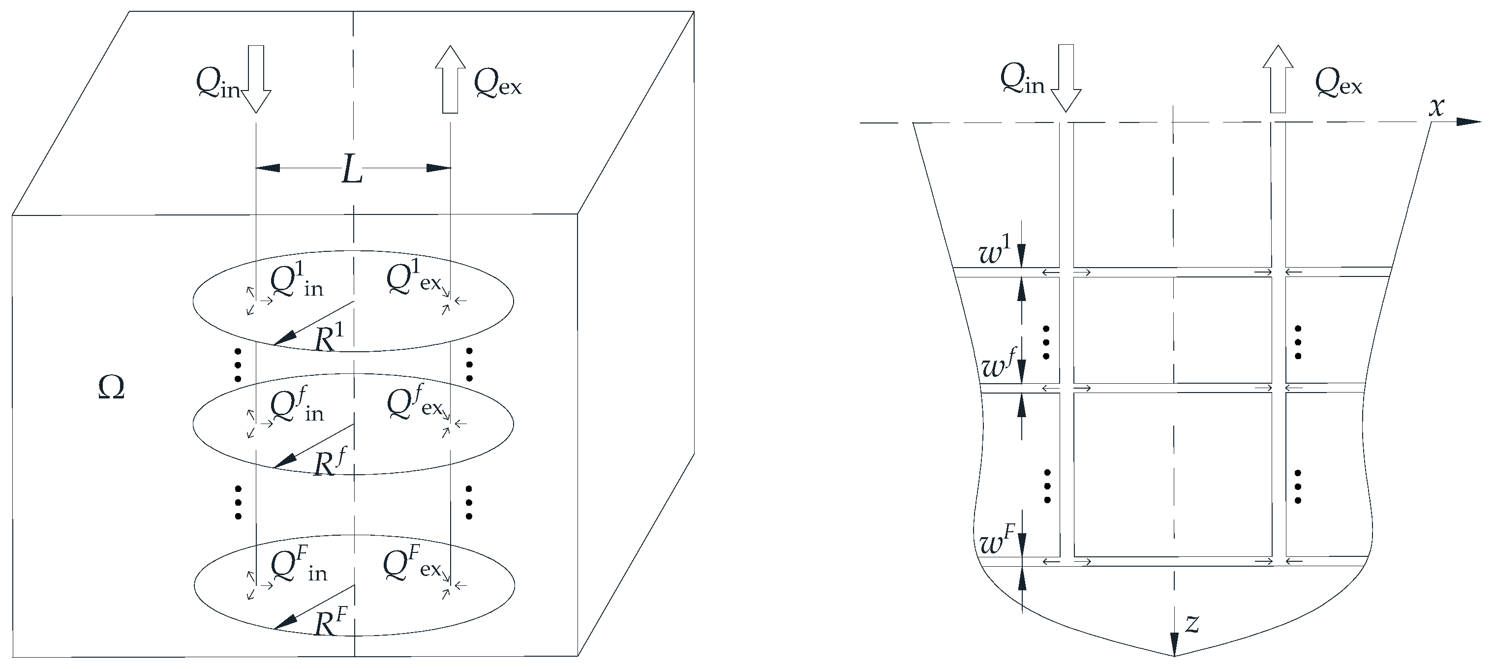
In this study, a multi-fracture EGS model was built based on the geometry suggested by Ref. [17]. In Figure 1, multiple horizontal disc-shaped fractures located in the center of a reservoir connect the injection and production wells. Due to the low permeability of the rock matrix, the leak-off is assumed to be negligible; thus, the heat propagates by conduction in the rock matrix and by convection within fractures. When time t > 0, cold water with a constant temperature T_in and a constant injection rate Q_in is injected into the system with the rock’s initial temperature of T₀. The hot water with a constant production rate Q_ex is pumped out at the same time. Some geometric parameters of the model are defined as follow: the radii of the wells are r_w; the separation between two wells is L; the number of fractures is F.

We also mention some assumptions for the physical model.

• The fracture water is incompressible, and the rock matrix is impermeable and homogenous.
• The thermal properties of the rock matrix and fracture water are independent of temperature variation.
• The aperture of the fractures remains uniform and invariant without considering the deformation induced by hydro-mechanical coupling or thermo-mechanical interaction. Due to the fact that the fracture aperture is relatively small compared to the fracture surface, each fracture is simplified as a plane that coincides with its axisymmetric surface.
• The heat transfer coefficient between the rock matrix and fracture water is infinite, which means that the temperature of the fracture water is equal to that of the rock matrix at the fracture surfaces.
• There is steady-state water flow in the fractures because the heat exchange in a geothermal reservoir is a long-term process.

2.1. Water Flow in Fractures

The water flow in the fth fracture is assumed to obey Darcy’s law [15]:

$$\nabla p^f\left({\mathit{x}}^f\right)=-\frac{{\mathsf{\pi }}^2{\mu }^f}{w^{f3}}{\mathit{q}}^f\left({\mathit{x}}^f\right),{\mathit{x}}^f\in A^f$$

(1)

where the superscript f denotes the fracture plane f, ∇ is the gradient operator, x^f is the point (x^f, y^f, z^f), q^f is the water discharge, p^f is the hydraulic pressure in the fracture, μ^f is the water viscosity, w^f is the fracture aperture, and A^f is the fracture plane area.

The water continuity equation within the fth fracture is expressed as:

$$\nabla ·{\mathit{q}}^f\left({\mathit{x}}^f\right)=Q_{\mathrm{ex}}^f\delta \left({\mathit{x}}^f-{\mathit{x}}_{\mathrm{ex}}^f\right)-Q_{\mathrm{in}}^f\delta \left({\mathit{x}}^f-{\mathit{x}}_{\mathrm{in}}^f\right)$$

(2)

where ∇· is the divergence operator, δ(·) is the Dirac delta function, $Q_{\mathrm{in}}^f$ is the flow rate at the injection well located at ${\mathit{x}}_{\mathrm{in}}^f$ = ($x_{\mathrm{in}}^f$, $y_{\mathrm{in}}^f$, $y_{\mathrm{in}}^f$), and $Q_{\mathrm{ex}}^f$ is the flow rate at the production well located at ${\mathit{x}}_{\mathrm{ex}}^f$ = ($x_{\mathrm{ex}}^f$, $y_{\mathrm{ex}}^f$, $z_{\mathrm{ex}}^f$).

Substituting Equation (1) to Equation (2) yields

$${\nabla }^2{p}^f\left({\mathit{x}}^f\right)=\frac{{\mathsf{\pi }}^2{\mu }^f}{w^{f3}}\left[Q_{\mathrm{ex}}^f\delta \left({\mathit{x}}^f-{\mathit{x}}_{\mathrm{ex}}^f\right)-Q_{\mathrm{in}}^f\delta \left({\mathit{x}}^f-{\mathit{x}}_{\mathrm{in}}^f\right)\right].$$

(3)

where ∇² is the Laplace operator.

For the water flow in the fth fracture, the following boundary condition is used:

$$\begin{array}{l}\frac{\partial p^f\left({\mathit{x}}^f\right)}{\partial n^f\left({\mathit{x}}^f\right)}=0,{\mathit{x}}^f\in \partial A^f\\ Q_{\mathrm{in}}^f=Q_{\mathrm{ex}}^f=\frac{Q_{\mathrm{in}}}{F}=\frac{Q_{\mathrm{ex}}}{F}\end{array}\}.$$

(4)

where ∂A^f is the boundary of the fracture, and n^f the outward normal of ∂A^f.

Based on the hypothesis that the fracture geometry including the radius and aperture is uniform, we can obtain the exact solution of the water discharge in the fth fracture by using the superposition procedure [18]:

$$q_x^f\left({\mathit{x}}^f\right)={\displaystyle \sum _{i=1}^2\frac{Q_i^f}{2\mathsf{\pi }}\left[\frac{x-x_i^f}{{\left(x-x_i^f\right)}^2+{\left(y-y_i^f\right)}^2}+\frac{r_{\mathrm{w}}^2\left(x{r}_{\mathrm{w}}^2-x_i^f{R}^{f2}\right)}{{\left(x{r}_{\mathrm{w}}^2-x_i^f{R}^{f2}\right)}^2+{\left(y{r}_{\mathrm{w}}^2-y_i^f{R}^{f2}\right)}^2}\right]},$$

(5)

$$q_y^f\left({\mathit{x}}^f\right)={\displaystyle \sum _{i=1}^2\frac{Q_i^f}{2\mathsf{\pi }}\left[\frac{y-y_i^f}{{\left(x-x_i^f\right)}^2+{\left(y-y_i^f\right)}^2}+\frac{r_{\mathrm{w}}^2\left(y{r}_{\mathrm{w}}^2-y_i^f{R}^{f2}\right)}{{\left(x{r}_{\mathrm{w}}^2-x_i^f{R}^{f2}\right)}^2+{\left(y{r}_{\mathrm{w}}^2-y_i^f{R}^{f2}\right)}^2}\right]}.$$

(6)

where $Q_i^f$ is the flow rate at the ith well located at ($x_i^f$, $y_i^f$, $z_i^f$). The sign is negative for injection and positive for production. R^f is the radius of the fracture.

2.2. Heat Transfer in Fractures

According to Cheng et al. [11], the heat transfer within fractures contains four components, i.e., heat storage, dispersion, convection, and conduction between the fracture water and the rock matrix. Due to the relatively large convection velocity, the heat storage and dispersion can be ignored. Thus, the heat transport in the fth fracture can be expressed as:

$${\rho }_{\mathrm{w}}{c}_{\mathrm{w}}{\mathit{q}}^f\left({\mathit{x}}^f\right)·\nabla T^f\left({\mathit{x}}^f,t\right)+q_h^f\left({\mathit{x}}^f,t\right)=0$$

(7)

where ρ_w is the water density, c_w is the water-specific heat, and $q_{\mathrm{h}}^f$ is the heat transfer rate between the fracture water and the rock matrix.

Assuming that temperature is continuous across fracture surfaces, the heat transfer rate in Equation (7) can be expressed as [19]:

$$q_{\mathrm{h}}^f\left({\mathit{x}}^f,t\right)=-2{\lambda }_{\mathrm{r}}{\frac{\partial T\left(\mathit{x},t\right)}{\partial z}|}_{z=z^f}$$

(8)

where λ_r is the thermal conductivity of the rock matrix.

2.3. Heat Transfer in the Rock Matrix

In a low-permeability rock matrix, the heat transfer dominated by conduction can be expressed as:

$${\lambda }_{\mathrm{r}}{\nabla }^{2}T\left(\mathit{x},t\right)={\rho }_{\mathrm{r}}{c}_{\mathrm{r}}\frac{\partial T\left(\mathit{x},t\right)}{\partial t},\mathit{x}\in \mathsf{\Omega }$$

(9)

where ρ_r is the rock matrix density and c_r is the rock matrix specific heat.

2.4. Initial and Boundary Condition

The initial and boundary conditions for the system are:

$$\begin{array}{l}T\left(\mathit{x},0\right)=T_0,\mathit{x}\subseteq \mathsf{\Omega }\\ T\left(\mathit{x},t\right)=T_{\mathrm{in}},\mathit{x}={\mathit{x}}_{\mathrm{in}}^f\\ T\left(\mathit{x},t\right)=T_0,\mathit{x}\to \pm \infty \end{array}\}.$$

(10)

2.5. Numerical Formation

2.5.1. Integral Equation Method

The temperature increment at location x and time t induced by an instantaneous unit point source at location x′ and time t′ < t is [20]:

$$\theta \left(\mathit{x}-{\mathit{x}}^{\prime },t-t^{\prime }\right)=\sqrt{\frac{{\rho }_{\mathrm{r}}{c}_{\mathrm{r}}}{{\left[4\mathsf{\pi }{\lambda }_{\mathrm{r}}\left(t-t^{\prime }\right)\right]}^3}}\exp \left(\frac{-{\rho }_{\mathrm{r}}{c}_{\mathrm{r}}{r}^2}{4{\lambda }_{\mathrm{r}}\left(t-t^{\prime }\right)}\right).$$

(11)

where $r=\sqrt{{\left(x-x^{\prime }\right)}^2+{\left(y-y^{\prime }\right)}^2+{\left(z-z^{\prime }\right)}^2}$.

Equation (11) is the temporal Green function of Equation (9). The heat transfer rate in Equation (8) is regarded as a heat sink when the fracture water is colder than the rock matrix. Taking into account heat sinks at all fracture planes, the resultant temperature in the reservoir at time t is:

$$T\left(\mathit{x},t\right)={\displaystyle \sum _{f=1}^F{\displaystyle {\int }_0^t{\displaystyle {\int }_{A^f}{q}_{\mathrm{h}}^f\left({\mathit{x}}^f,t^{\prime }\right)\theta \left(\mathit{x}-{\mathit{x}}^f,t-t^{\prime }\right)\mathrm{d}{A}^f}\mathrm{d}{t}^{\prime }}}+T_0.$$

(12)

Applying Equation (12) at the fth fracture plane yields

$$T^f\left({\mathit{x}}^f,t\right)={\displaystyle \sum _{i=1}^F{\displaystyle {\int }_0^t{\displaystyle {\int }_{A^i}{q}_{\mathrm{h}}^i\left({\mathit{x}}^i,t^{\prime }\right)\theta \left({\mathit{x}}^f-{\mathit{x}}^i,t-t^{\prime }\right)\mathrm{d}{A}^i}\mathrm{d}{t}^{\prime }}}+T_0.$$

(13)

Using the convolution algorithm [21] for Equation (13) yields

$$T^f\left({\mathit{x}}^f,t\right)={\displaystyle \sum _{i=1}^F{\displaystyle \sum _{n=1}^N{q}_{\mathrm{h}}^f\left({\mathit{x}}^f,t_n\right){\displaystyle {\int }_{A^i}{\theta }_{N-n+1}^{\mathrm{ch}}\left({\mathit{x}}^f-{\mathit{x}}^i\right)\mathrm{d}{A}^i}}}+T_0$$

(14)

where the time from 0 to t is divided into N equal intervals of Δt, ${\theta }_n^{\mathrm{ch}}$ is the integration of θ from time t_N−n to time t_N−n+1, and is expressed as:

$${\theta }_n^{\mathrm{ch}}\left(\mathit{x}-{\mathit{x}}^{\prime }\right)={\displaystyle {\int }_{t_{N-n}}^{t_{N-n+1}}\theta \left(\mathit{x}-{\mathit{x}}^{\prime },t-t^{\prime }\right)\mathrm{d}{t}^{\prime }}=\frac{1}{4\mathsf{\pi }{\lambda }_{\mathrm{r}}r}\left[\mathrm{erfc}\left(\frac{r}{\sqrt{4{\alpha }_{\mathrm{r}}{t}_n}}\right)-\mathrm{erfc}\left(\frac{r}{\sqrt{4{\alpha }_{\mathrm{r}}{t}_{n-1}}}\right)\right].$$

(15)

where α_r = λ_r/ρ_rc_r is the heat diffusivity of the rock matrix and erfc (·) is the complementary error function, which approximates to zero when the expression in the brackets approaches infinity.

Equation (14) with the initial and boundary conditions in Equation (10) can be used to obtain the temperature and heat transfer rate at each fracture plane.

2.5.2. Numerical Calculation

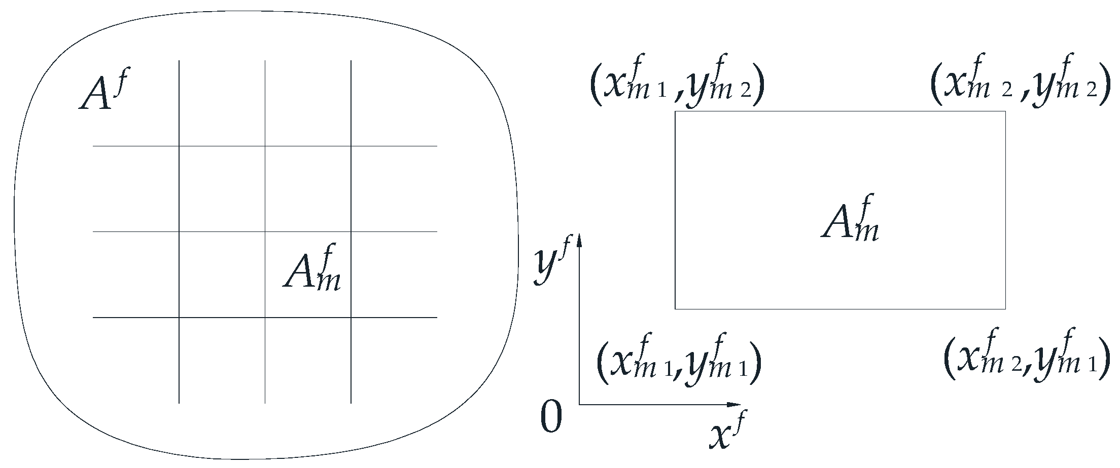
Fracture planes are discretized into a number of four–noded quadrilateral elements. For the fth fracture plane, there are M^f elements and K^f nodes as shown in Figure 2.

The following interpolations for any element m are used:

$$T_m^f=\mathit{N}{\mathit{T}}_m^f,q_{\mathrm{h}m}^f=\mathit{N}{\mathit{q}}_{\mathrm{h}m}^f$$

(16)

where the subscript m denotes the element m, ${\mathit{T}}_m^f$ is the vector of nodal temperature, ${\mathit{q}}_{\mathrm{h}m}^f$ is the vector of the nodal heat transfer rate, and N is the vector of interpolation functions.

Substituting Equation (16) into Equation (14) yields

$$T^f\left({\mathit{x}}^f,t\right)\approx {\displaystyle \sum _{i=1}^F{\displaystyle \sum _{n=1}^N{\displaystyle \sum _{m=0}^{M^i}{\displaystyle {\int }_{A_m^i}\mathit{N}{\theta }_{N-n+1}^{\mathrm{ch}}\left({\mathit{x}}^f-{\mathit{x}}^i\right)\mathrm{d}{A}_m^i}}{\mathit{q}}_{\mathrm{h}m}^i\left(t_n\right)}}+T_0.$$

(17)

Applying Equation (17) to all element nodes at the fth fracture plane yields

$${\mathit{T}}^f\left(t\right)={\displaystyle \sum _{i=1}^F\left[{\mathit{B}}^{f,i}{\mathit{q}}_{\mathrm{h}}^i\left(t\right)+{\mathit{C}}^{f,i}\right]}+{\mathit{D}}^f$$

(18)

where, specifically,

$${\mathit{B}}^{f,i}={\displaystyle \sum _{m=1}^{M^i}\left[\begin{array}{c}{\displaystyle {\int }_{A_m^i}\mathit{N}{\theta }_1^{\mathrm{ch}}\left({\mathit{x}}_1^f-{\mathit{x}}^i\right)\mathrm{d}{A}_m^i}\\ {\displaystyle {\int }_{A_m^i}\mathit{N}{\theta }_1^{\mathrm{ch}}\left({\mathit{x}}_2^f-{\mathit{x}}^i\right)\mathrm{d}{A}_m^i}\\ ⋮\\ {\displaystyle {\int }_{A_m^i}\mathit{N}{\theta }_1^{\mathrm{ch}}\left({\mathit{x}}_{K^f}^f-{\mathit{x}}^i\right)\mathrm{d}{A}_m^i}\end{array}\right]},$$

(19)

$${\mathit{C}}^{f,i}={\displaystyle \sum _{n=1}^{N-1}{\displaystyle \sum _{m=1}^{M^i}\left[\begin{array}{c}{\displaystyle {\int }_{A_m^i}\mathit{N}{\theta }_{N-n+1}^{\mathrm{ch}}\left({\mathit{x}}_1^f-{\mathit{x}}^i\right)\mathrm{d}{A}_m^i}\\ {\displaystyle {\int }_{A_m^i}\mathit{N}{\theta }_{N-n+1}^{\mathrm{ch}}\left({\mathit{x}}_2^f-{\mathit{x}}^i\right){d}{A}_m^i}\\ ⋮\\ {\displaystyle {\int }_{A_m^i}N{\theta }_{\mathit{N}-n+1}^{\mathrm{ch}}\left({\mathit{x}}_{K^f}^f-{\mathit{x}}^i\right)\mathrm{d}{A}_m^i}\end{array}\right]}}{\mathit{q}}_{{h}}^i\left(t_n\right),$$

(20)

$${\mathit{D}}^f={\left[T_0\left({\mathit{x}}_1^f\right),T_0\left({\mathit{x}}_2^f\right),\cdots ,T_0\left({\mathit{x}}_{K^f}^f\right)\right]}^{\mathrm{T}}.$$

(21)

where the superscript T denotes the transpose of a vector.

Usually, the conventional Galerkin finite element method for the convection-dominated problems is corrupted by spurious node-to-node oscillations. In order to reduce the numerical oscillations, the Streamline upwind/Petrov–Galerkin method [22] is used for Equation (7), which can be written as follows:

$${\mathit{E}}^f{\mathit{T}}^f\left(t\right)+{\mathit{F}}^f{\mathit{q}}_{\mathrm{h}}^f\left(t\right)=\mathbf{0},$$

(22)

where

$${\mathit{E}}^f={\rho }_{\mathrm{w}}{c}_{\mathrm{w}}{\displaystyle \sum _{m=1}^{M^f}{\displaystyle {\int }_{A_m^f}{\displaystyle \sum _{i=1}^2\left({\mathit{N}}^{\mathrm{T}}+{\overline{k}}_{x_{i}m}^f\frac{\partial {\mathit{N}}^{\mathrm{T}}}{\partial x_i^f}\right)\mathit{N}{\mathit{q}}_{x_i}^f\frac{\partial \mathit{N}}{\partial x_i^f}}\mathrm{d}{A}_m^f}},x_i=x,y,$$

(23)

$${\overline{k}}_{x_{i}m}^f=\frac{q_{x_{i}m}^{\mathrm{c}f}}{2}{\displaystyle \sum _{k=1}^2\frac{q_{x_{k}m}^{\mathrm{c}f}\Delta x_{km}^f}{q_{xm}^{\mathrm{c}f2}+q_{ym}^{\mathrm{c}f2}}\left(\coth \left(\frac{q_{x_{k}m}^{\mathrm{c}f}\Delta x_{km}^f}{2w^f{k}_{\mathrm{w}}}\right)-\frac{2w^f{k}_{\mathrm{w}}}{q_{x_{k}m}^{\mathrm{c}f}\Delta x_{km}^f}\right)},x_k=x,y,$$

(24)

$${\mathit{F}}^f={\displaystyle \sum _{m=1}^{M^f}{\displaystyle {\int }_{A_m^f}{\mathit{N}}^{\mathrm{T}}\mathit{N}\mathrm{d}{A}_m^f}}.$$

(25)

in which Δ$x_{km}^f$ is the element length in x_k direction, $q_{x_{k}m}^{\mathrm{c}f}$ is the water discharge at the center of the element, and k_w is the water diffusivity.

Substituting Equation (18) to Equation (22) yields:

$$\left({\mathit{E}}^f{\mathit{B}}^{f,f}+{\mathit{F}}^f\right){\mathit{q}}_{\mathrm{h}}^f\left(t\right)+{\displaystyle \sum _{i=1,i\ne f}^F{\mathit{E}}^f{\mathit{B}}^{f,i}{\mathit{q}}_{\mathrm{h}}^i\left(t\right)}=-{\mathit{E}}^f\left({\displaystyle \sum _{i=1}^F{\mathit{C}}^{f,i}}+{\mathit{D}}^f\right).$$

(26)

The heat transfer rate ${\mathit{q}}_{\mathrm{h}}^f(t)$ can be obtained by solving Equation (26). Thereafter, Equation (12) can be discretized as presented in this section to calculate the temperature of the fracture water and rock matrix.

3. Results and Discussion

3.1. Verification of the Temporal Semi-Analytical Method

3.1.1. Injection into an Infinite Rectangular Fracture

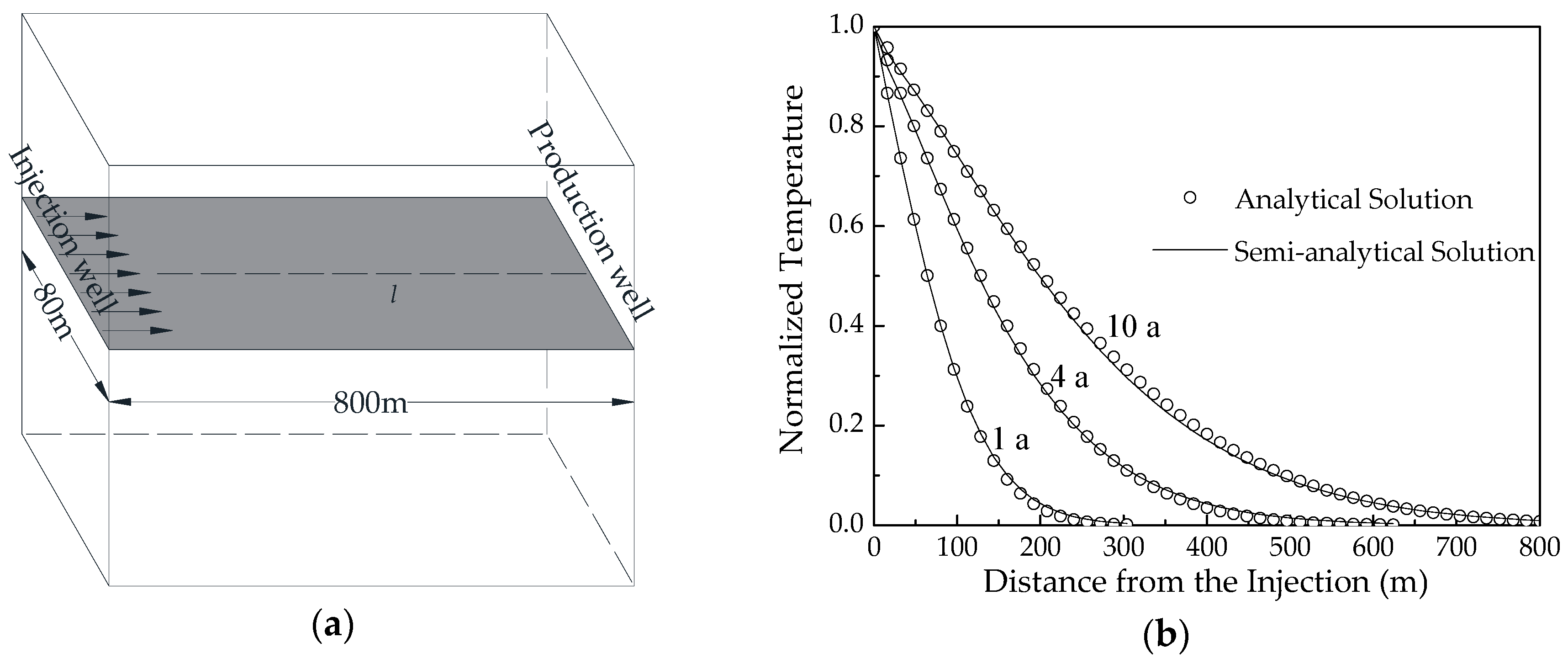
To verify the model proposed, we considered the problem of one-dimensional water injection into an infinite rectangular-shaped fracture as shown in Figure 3a. The length, width, and aperture of the fracture were 800 m, 80 m, and 0.003 m, respectively. The unit-width discharge was 1.5 × 10⁻⁵ m² s⁻¹. The parameters in

Table 1. Parameters used.

Parameters	Values	Parameters	Values
Water density ρw (Kg m−3)	1000	Water diffusivity kw (m2 s−1)	0.01
Rock density ρr (Kg m−3)	2650	Rock conductivity λr (W m−1 °C−1)	2.59
Water-specific heat cw (J kg−1 °C−1)	4180	Initial rock temperature T0 (°C−1)	90
Rock-specific heat cr (J kg−1 °C−1)	1000	Injected water temperature Tin (°C−1)	20

were used here. The temperature of line l located centrally in the fracture plane was calculated. Based on one-dimensional conduction in the rock matrix, the analytical solution for the normalized fracture water temperature is as follows [10]:

$$\frac{T-T_0}{T_{\mathrm{in}}-T_0}=\mathrm{erfc}\left[\left(\frac{{\lambda }_{\mathrm{r}}x}{{\rho }_{\mathrm{w}}{c}_{\mathrm{w}}q}+\frac{w}{4}\right)\sqrt{\frac{{\rho }_{\mathrm{r}}{c}_{\mathrm{r}}}{{\lambda }_{\mathrm{r}}t}}\right].$$

(27)

where x is the perpendicular distance from the interest point to the injection well, q is the unit-width discharge, and w is the fracture aperture. The other variables are as described above.

Figure 3b shows the comparison of the results for injection times of 1, 4, and 10 years. We observe that the difference between the two solutions is small. However, with the elapse of time, the difference becomes noticeable due to the different assumptions about conduction in the rock matrix.

3.1.2. Injection into an Infinite Radial Fracture

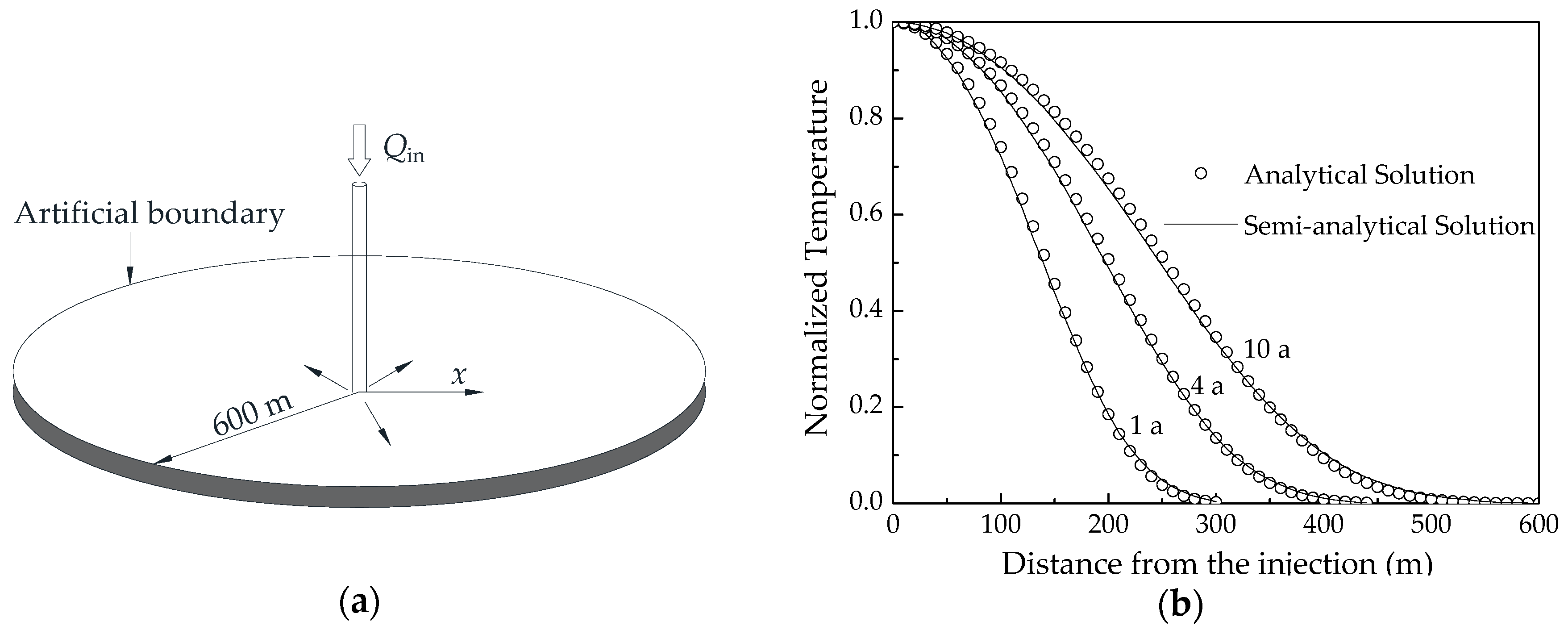
To validate the model presented, the heat transfer of radial flow through an infinite fracture was modeled. In Figure 4a, cold water was injected into the center of the fracture. Based on one-dimensional conduction in the rock matrix, the analytical solution for the normalized fracture water temperature is given as [23]:

$$\frac{T-T_0}{T_{\mathrm{in}}-T_0}=\mathrm{erfc}\left[\left(\frac{\mathsf{\pi }{\lambda }_{\mathrm{r}}{x}^2}{{\rho }_{\mathrm{w}}{c}_{\mathrm{w}}{Q}_{\mathrm{in}}}+\frac{w}{4}\right)\sqrt{\frac{{\rho }_{\mathrm{r}}{c}_{\mathrm{r}}}{{\lambda }_{\mathrm{r}}t}}\right].$$

(28)

where x is the radial distance from the interest point to the injection well and Q_in is the injection rate; the other variables are as described above.

The case that is shown in Figure 4a with an injection rate of 0.015 m³ s⁻¹, wellbore radius of 0.1 m, and fracture aperture of 0.003 m was analyzed. In order to reduce the impact of truncated boundaries, the radius of the fracture was set at 600 m. Other parameters are listed in Table 1. Figure 4b illustrates the comparison of results for injection times of 1, 4, and 10 years. A good match is observed between the solutions from the present model and the analytical one.

3.2. Multi-Fracture EGS

In this section, the temporal semi-analytical method was applied to investigate the effects of fracture spacing and fracture number on the response of an EGS. Without loss of generality, the fractures were equidistant. We assumed that the injection rate was 0.05 m³ s⁻¹, wellbore radius 0.1 m, wellbore spacing 60 m, fracture radius 50 m, and fracture aperture 0.001 m. Each fracture plane was discretized spatially by 1992 quadratic elements. Other parameters are shown in Table 1.

3.2.1. Effects of the Fracture Spacing

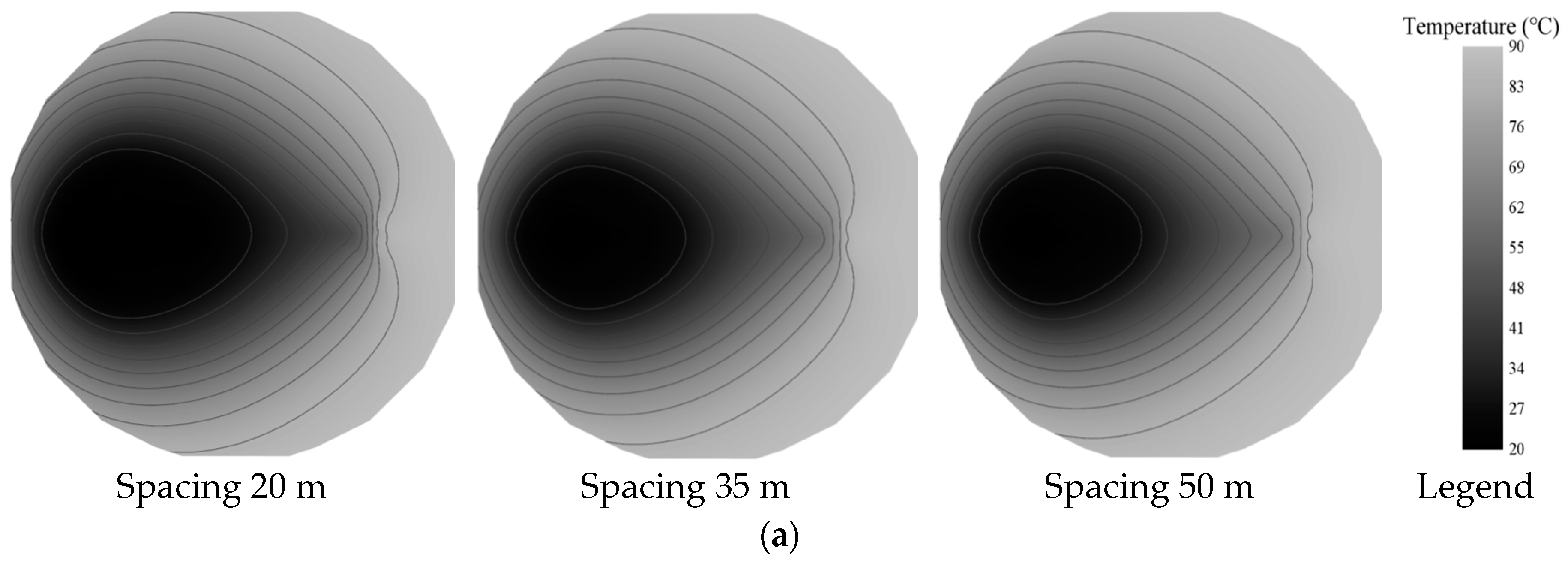
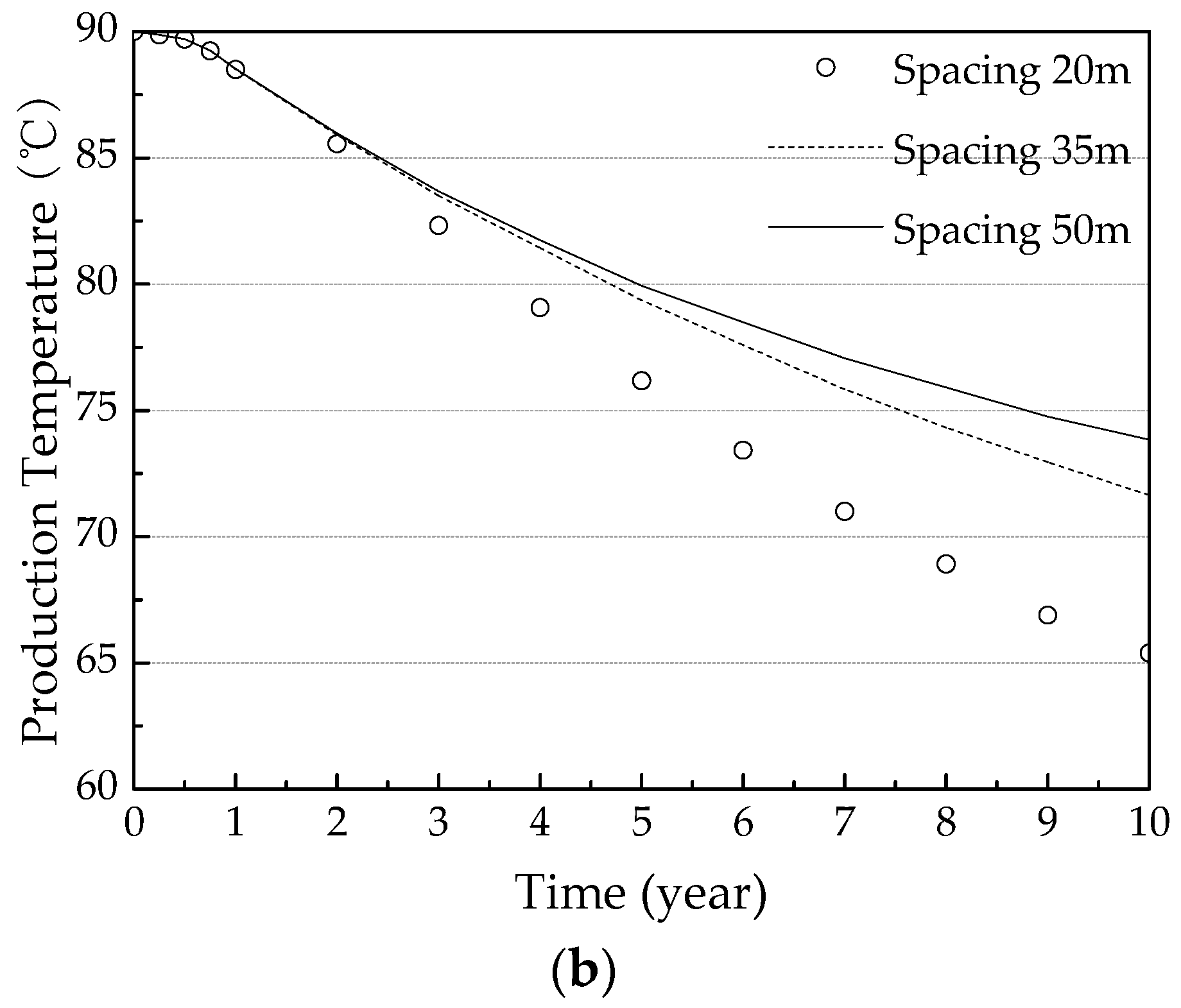
Assuming that there were two parallel fractures in Figure 1, we aimed at probing the influence of fracture spacing on fracture water temperature. The spacing between the two fractures ranged from 20 m to 50 m. For three cases with fracture spacings of 20 m, 35 m, and 50 m, the fracture temperature distribution after 5 years of extraction and the production temperature variation within 10 years are shown in Figure 5. With increasing the fracture spacing, the production temperature rose because the thermal interplay between the two fractures decreased correspondingly, while its relative increment declined. When the fracture spacing was increased from 30 m to 50 m, the relative increasing rate of the production temperature was lower than 3%. We can indicate that a spacing larger than 50 m is too large for thermal interaction, which is compatible with the results obtained by Vik et al. [3].

3.2.2. Effects of the Fracture Number

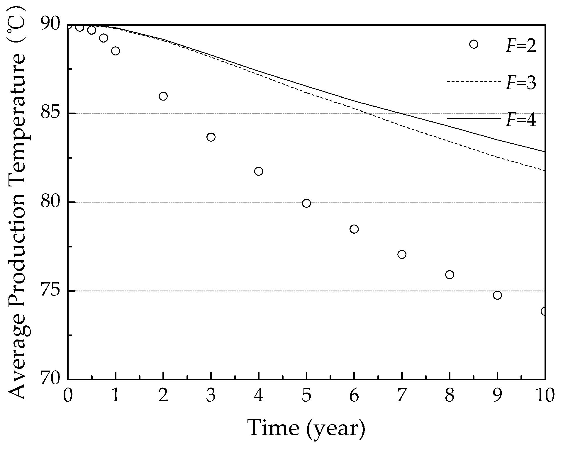
Assuming that the distance between the top fracture and the bottom one was 50 m in Figure 1, more horizontal fractures were added in the rock between them. Three cases were studied where the number of fractures was set to 2, 3, and 4, and correspondingly the uniform spacings were 50 m, 25 m, and 50/3 m. Figure 6 illustrates the average temperature of the water pumped from all fractures in each project, respectively. As the number of fractures increased, the production temperature rose because the contacting area between the fracture water and rock matrix expanded correspondingly, while its relative increment decreased. When the fracture number was increased from 3 to 4, the relative increasing rate of the production temperature was lower than 2%. We can observe that the optimal fracture number is 4, which approaches the smallest value of 6 proposed by Wu et al. [17]. In addition, the comparison between Figure 5b and Figure 6 reveals that increasing the fracture number improves the heat extracted more efficiently than does enlarging the fracture spacing.

4. Conclusions

In this study, a temporal semi-analytical model was developed to predict the heat exploited from an EGS with multiple parallel fractures. This model considers the three-dimensional conduction in the rock matrix and the finite scale of fractures. The solution was applied to investigate the effects of fracture spacing and fracture number on the production temperature of an EGS. The results show the following:

• The temporal semi-analytical method provides an accurate solution and, thus, can serve as a benchmark for numerical methods.
• The fracture spacing and fracture number are two key factors controlling the heat extraction from an EGS. Increasing the fracture spacing maintains the production temperature by decreasing the thermal interaction between fractures. A multi-fracture also extends the life of a geothermal reservoir by increasing the contacting area between the fracture water and rock matrix. In terms of improving heat exploitation, increasing the fracture number is more efficient than increasing fracture spacing.
• The proposed method is efficient in calculations and is applicable to the design and optimization of an EGS.

References

- Luo, J.; Luo, Z.Q.; Xie, J.H.; Xia, D.S.; Huang, W.; Shao, H.B.; Xiang, W.; Rohn, J. Investigation of shallow geothermal potentials for different types of ground source heat pump systems (GSHP) of Wuhan city in China. Renew. Energy 2018, 118, 230–244. [Google Scholar] [CrossRef]
- Olasolo, P.; Juárez, M.C.; Morales, M.P.; D’Amico, S.; Liarte, I.A. Enhanced geothermal systems (EGS): A review. Renew. Sustain. Energy Rev. 2016, 56, 133–144. [Google Scholar] [CrossRef]
- Vik, H.S.; Salimzadeh, S.; Nick, H.M. Heat Recovery from Multiple-Fracture Enhanced Geothermal Systems: The Effect of Thermoelastic Fracture Interactions. Renew. Energy 2018, 121, 606–622. [Google Scholar] [CrossRef]
- Yao, J.; Zhang, X.; Sun, Z.X.; Huang, Z.Q.; Li, Y.; Xin, Y.; Yan, X.; Liu, W.Z. Numerical simulation of the heat extraction in 3D-EGS with thermal-hydraulic-mechanical coupling method based on discrete fractures model. Geothemics 2018, 74, 19–34. [Google Scholar] [CrossRef]
- Xia, Y.D.; Plummer, M.; Mattson, E.; Podgorney, R.; Ghassemi, A. Design, modeling, and evaluation of a doublet heat extraction model in enhanced geothermal systems. Renew. Energy 2017, 105, 232–247. [Google Scholar] [CrossRef]
- Galgaro, A.; Farina, Z.; Emmi, G.; Crali, M.D. Feasibility analysis of a Borehole Heat Exchanger (BHE) array to be installed in high geothermal flux area: The case of the Euganean Thermal Basin, Italy. Renew. Energy 2015, 78, 93–104. [Google Scholar] [CrossRef]
- Kelkar, S.; Lewis, K.; Karra, S.; Zyvoloski, G.; Rapaka, S.; Viswanathan, H.; Mishra, P.K.; Chu, S.; Coblentz, D.; Pawar, R. A simulator for modeling coupled thermo-hydro-mechanical processes in subsurface geological media. Int. J. Rock Mech. Min. 2014, 70, 569–580. [Google Scholar] [CrossRef]
- Zeng, Y.C.; Su, Z.; Wu, N.Y. Numerical simulation of heat production potential from hot dry rock by water circulating through two horizontal wells at Desert Peak geothermal field. Energy 2013, 56, 92–107. [Google Scholar] [CrossRef]
- Huang, W.B.; Cao, W.J.; Jiang, F.M. Heat extraction performance of EGS with heterogeneous reservoir: A numerical evaluation. Int. J. Heat Mass. Transf. 2017, 108, 645–657. [Google Scholar] [CrossRef]
- Lauwerier, H.A. The transport of heat in an oil layer caused by the injection of hot fluid. Appl. Sci. Res. Sect. A 1955, 5, 145–150. [Google Scholar] [CrossRef]
- Cheng, A.H.D.; Ghassemi, A.; Detournay, E. Integral equation solution of heat extraction from a fracture in hot dry rock. Int. J. Numer. Anal. Methods Geomech. 2001, 25, 1327–1338. [Google Scholar] [CrossRef]
- Ghassemi, A.; Tarasovs, S.; Cheng, A.H.D. An integral equation for three-dimensional heat extraction from planar fracture in hot dry rock. Int. J. Numer. Anal. Methods Geomech. 2003, 27, 989–1004. [Google Scholar] [CrossRef]
- Xiang, Y.Y.; Guo, J.Q. A Laplace transform and Green function method for calculation of water flow and heat transfer in fractured rocks. Rock Soil Mech. 2011, 32, 333–340. [Google Scholar]
- Zhang, Y.; Xiang, Y.Y. A semi-analytical method for calculation of three-dimensional water flow and heat transfer in single-fracture rock with distributed heat sources. Rock Soil Mech. 2013, 34, 685–695. [Google Scholar]
- Zhou, X.X.; Ghassemi, A.; Cheng, A.H.D. A three-dimensional integral equation model for calculating poro- and thermoelastic stresses induced by cold water injection into a geothermal reservoir. Int. J. Numer. Anal. Methods Geomech. 2009, 33, 1613–1640. [Google Scholar] [CrossRef]
- Abbasi, M.; Khazali, N.; Sharifi, M. Analytical model for convection-conduction heat transfer during water injection in fractured geothermal reservoirs with variable rock matrix block size. Geothermics 2017, 69, 1–14. [Google Scholar] [CrossRef]
- Wu, B.S.; Zhang, X.; Jeffrey, R.G.; Bunger, A.P.; Jia, S.P. A simplified model for heat extraction by circulating fluid through a closed-loop multiple-fracture enhanced geothermal system. Appl. Energy 2016, 183, 1664–1681. [Google Scholar] [CrossRef]
- Liggett, J.A.; Liu, P.L.F. The Boundary Integral Equations Method for Porous Media Flow; George Allen & Unwin: London, UK, 1983. [Google Scholar]
- Ghassemi, A.; Zhou, X.X. A three-dimensional thermo-poroelastic model for fracture response to injection/extraction in enhanced geothermal systems. Geothemics 2011, 40, 39–49. [Google Scholar] [CrossRef]
- Xiang, Y.Y. Fundamental Theory of Groundwater Mechanics; Science Press: Beijing, China, 2011. [Google Scholar]
- Dargush, G.; Banerjee, P.K. A time domain boundary element method for poroelasticity. Int. J. Numer. Meth. Eng. 1989, 28, 2423–2449. [Google Scholar] [CrossRef]
- Brooks, A.N.; Hughes, T.J.R. Streamline upwind/Petrov-Galerkin formulations for convection dominated flows with particular emphasis on the incompressible Navier-Stokes equations. Comput. Method. Appl. M 1982, 32, 19–259. [Google Scholar] [CrossRef]
- Mossop, A.P. Seismicity, subsidence and strain at the Geysers geothermal field. Ph.D. Thesis, Stanford University, Location of University, Stanford, CA, USA, 2001. [Google Scholar]
Figure 1.
Geometry of the model with multi-parallel disc-shaped fractures and dipole wells.
Figure 2.
Discretization of the fth fracture plane.
Figure 3.
(a) Water flows through an infinite rectangular fracture in which the left and right sides are the positions of the injection and production wells, respectively [10]; (b) Normalized temperature increment distribution along line l.
Figure 4.
(a) Injection into an infinite radial fracture [23]; (b) Normalized temperature increment distribution in the radial fracture.
Figure 5.
Effect of various fracture spacings on fracture temperature: (a) Fracture temperature distribution after 5 years of extraction; (b) Temperature breakthrough curves.
Figure 6.
Average production temperature for a fracture number of 2, 3, and 4.