A Novel Multi-Population Based Chaotic JAYA Algorithm with Application in Solving Economic Load Dispatch Problems


1
Department of Electrical Engineering, Yeungnam University, Gyeongsan 38541, Korea
2
Department of Electronic Information and Electrical Engineering, Anyang Institute of Technology, Anyang 455000, China
*
Author to whom correspondence should be addressed.
Energies 2018, 11(8), 1946; https://doi.org/10.3390/en11081946
Submission received: 1 July 2018
/
Revised: 20 July 2018
/
Accepted: 22 July 2018
/
Published: 26 July 2018
(This article belongs to the Special Issue Optimization Methods Applied to Power Systems)
Abstract
:The economic load dispatch (ELD) problem is an optimization problem of minimizing the total fuel cost of generators while satisfying power balance constraints, operating capacity limits, ramp-rate limits and prohibited operating zones. In this paper, a novel multi-population based chaotic JAYA algorithm (MP-CJAYA) is proposed to solve the ELD problem by applying the multi-population method (MP) and chaotic optimization algorithm (COA) on the original JAYA algorithm to guarantee the best solution of the problem. MP-CJAYA is a modified version where the total population is divided into a certain number of sub-populations to control the exploration and exploitation rates, at the same time a chaos perturbation is implemented on each sub-population during every iteration to keep on searching for the global optima. The proposed MP-CJAYA has been adopted to ELD cases and the results obtained have been compared with other well-known algorithms reported in the literature. The comparisons have indicated that MP-CJAYA outperforms all the other algorithms, achieving the best performance in all the cases, which indicates that MP-CJAYA is a promising alternative approach for solving ELD problems.
1. Introduction
With the issues of global warming and depletion of classical fossil fuels, saving energy and reducing the operational cost have become the key topics in power systems nowadays. The economic load dispatch problem (ELD) is a crucial issue of power system operation that minimizes the operational cost while satisfying a set of physical and operational constraints imposed by generators and system limitations [1]. A large number of conventional optimization methods have been applied successfully for solving the ELD problem such as gradient method [2], lambda iteration method [3], semi-definite programming [4], quadratic programming [5], dynamic programming [6], Lagrangian relaxation method [7] and linear programming [8]. However, they suffer from difficulties when dealing with problems with nonconvex objective function and complex constraints, which tends to exhibit highly non-linear, non-convex and non-smooth characteristics with a number of local optima [9].
To overcome these drawbacks, meta-heuristic methods are proposed, such as genetic algorithm (GA) [10], particle swarm optimization (PSO) [11], tabu search (TS) [12], artificial bee colony algorithm (ABC) [13], firefly algorithm [14], harmony search (HS) [15] and teaching-learning-based optimization (TLBO) [16]. Additionally, hybrid meta-heuristic optimization approaches built by the combination between conventional methods and meta-heuristic methods or among the meta-heuristic methods have also been reported to deal with the ELD problem, such as DE-PSO method [17], HS-DE method [18], GA-PS-SQP algorithm [19] and Quantum-PSO method [20]. Even though hybrid methods offer much faster convergence rates, the combination may lead to increased numbers of parameters which causes more difficulties in selecting the proper value for each one. Hence, a new method with strong searching ability and less number of control parameters is needed.
The JAYA algorithm is a newly developed yet advanced heuristic algorithm for solving constrained and unconstrained optimization problems [21]. Different from other algorithms requiring for algorithm-specific parameters in addition to common parameters, the JAYA algorithm does not require any algorithm-specific parameters except for two common parameters named the population size (Npop) and the number of iteration (Niter). This significant benefit makes it popular in various real-world optimization problems such as optimum power flow [22], heat exchangers [23], photovoltaic models [24], thermal devices [25], MPPT of PV system [26], constrained mechanical design optimization [27], modern machining processes [28] and PV-DSTATCOM [29]. However, as a newly developed algorithm, the JAYA algorithm still has some disadvantages even though the number of parameters is less and the convergence rate is accelerated. Since there is only guidance as approach to get close to the best solution and get away from the worst solution, the population diversity may not be maintained efficiently, easily leading to local optimal solutions.
The multi-population based optimization method (MP) is applied for improving the search diversity by dividing the whole population into a certain number of sub-populations and distributing them throughout the search area so that the problem changes can be monitored more effectively. The MP method is aimed at maintaining population diversity during the search period by distributing different sub-populations to different search spaces. Each population is used to either intensify or diversifying the search process [30,31]. The interaction among the sub-populations occurs by dividing and merging process as long as a change in the solution is detected. Branke proposed a multi-population evolutionary algorithm in [32]. Turky and Abdullah proposed a multi-population electromagnetic algorithm and a multi-population harmony search algorithm in [33,34]. Nseef proposed a multi-population artificial bee colony algorithm in [35]. The published literature have demonstrated that employing MP method is useful for maintaining the population diversity when dealing with various problem changes.
Its worthy to be noted that the MP optimization method has superior behaviors because [36]:
- (1)
- By dividing the whole population into sub-populations, population diversity can be maintained since the sub-populations are located in different regions of the problem landscape.
- (2)
- With the ability to search various regions simultaneously, it is able to track the movement of optimum value more effectively.
- (3)
- Population-based optimization algorithms can be easily integrated with MP method.
At the same time the chaotic optimization algorithm (COA) which adopts chaotic sequences instead of random sequences is also employed here. Due to the non-repetitive characteristics of chaotic sequences, the COA can execute with shorter execution time and more robust mechanisms than stochastic ergodic searches that depending on random probabilities. It also has the feature of easy implementation in meta-heuristic algorithms, such as chaotic evolutionary algorithms [37], chaotic ant swarm optimization [38], chaotic harmony search algorithm [39], chaotic particle swarm optimization [40], chaotic firefly algorithm [41]. The choice of chaotic sequences is justified theoretically by their unpredictability, i.e., by their spread-spectrum characteristic, non-periodic, complex temporal behavior and ergodic properties. Simulation results from the abovementioned literature have demonstrated that the application of deterministic chaotic signals to meta-heuristic algorithms is a promising strategy in engineering applications. In this paper, COA has been applied twice:
- (1)
- During the initialization step, chaotic sequences generated by a chaotic map are used to initialize the initial solutions.
- (2)
- During the iteration step, COA is conducted to search further around the solution obtained by former algorithm to enhance the global convergence and to prevent to be trapped on local optima.
Based on the descriptions above, a novel multi-population based chaotic JAYA algorithm (MP-CJAYA) is proposed in this paper. It is a modified version of JAYA algorithm where the total population is divided into sub-populations by the MP method to control the exploration and exploitation rates, meanwhile a chaos perturbation is implemented on each sub-population during every iteration to keep on searching for the global optima. The MP-CJAYA algorithm is applied for solving the ELD cases with constraints including valve-point effects, power balance constraints, operating capacity limits, ramp-rate limits and prohibited operating zones. In all the experimented ELD cases, the proposed MP-CJAYA has produced the most competitive results.
The rest of this paper is arranged as follows: In Section 2, the problem formulation of ELD problem is constructed. The basic JAYA, the compared CJAYA and the proposed MP-CJAYA algorithms are described in Section 3. The experimental results and comparisons of MP-CJAYA with other algorithms are presented and analyzed in Section 4. Finally, the conclusions and future work are given in Section 5.
2. Problem Formulation
The ELD problem is described as an objective function to minimize the total fuel cost while satisfying different constraints, we adopt the problem formulation described in [16,42].
2.1. Objective Function
The objective function is to sum up all the costs of committed generators as expressed below:
where is the total generator number in power systems, is the cost function of generator with output .
Approximately, the cost function can be expressed as a quadratic polynomial by the following equation:
where , , are the cost coefficients of generator, which are constants.
In reality, a higher-order non-linearity rectified sinusoid contribution is usually added to the cost function to model the valve-point effect, which is given below:
where and are cost coefficients of generator due to valve-point effect, while is the minimum output for generator .
According to the discussion above, the objective function of ELD problem considering the valve-point effect can be represented as:
2.2. Constrained Functions
2.2.1. Power Losses
The total power generated by available units must equal to the summation of the demanded power and the system power loss, which can be formulated as:
where and is the value of the demanded power and the whole power loss in the system respectively. is calculated by Kron’s formula:
where , , are the loss coefficients that generally can be assumed to be constants under a normal operating condition.
2.2.2. Generating Capacity
The real output generated by a available unit must be ranged between its minimum limit and maximum limit:
where and are the minimum and maximum limits of generator.
2.2.3. Ramp Rate Limit
In practical circumstances, the output power can not be adjusted immediately, the operating range is restricted by the ramp-rate limit constraint expressed below:
where is the present power output, is the previous power output, and is the up-ramp and down-ramp limit of generator respectively.
2.2.4. Prohibited Operating Zones
For generator with prohibited operating zones (POZs), which are the sets of output power ranges where the generator can not work, the feasible operating zones are as discontinuous as follows:
where is the index of POZs, is the total number of POZs where , and are the lower and upper bounds of the POZ of the unit, respectively.
3. The Proposed MP-CJAYA Algorithm
Since the proposed MP-CJAYA algorithm is a hybrid of the basic JAYA, COA and MP methods, it is quite necessary to observe the relative strength of each constituent when solving the ELD problem, so three different algorithms are studied:
- (1)
- The basic JAYA algorithm: The classical JAYA algorithm with standard parameters; it is selected to compare its performance at solving different ELD cases with the other two algorithms.
- (2)
- The compared CJAYA algorithm: The basic JAYA algorithm combined by COA but without the MP method.
- (3)
- The proposed MP-CJAYA algorithm: The basic JAYA algorithm integrated with both the COA and MP methods.
3.1. The Basic JAYA Algorithm
The JAYA algorithm is a powerful heuristic algorithm proposed by Rao for solving optimization problems. It always attempts to get success to reach the best solution as well as move far away from the worst solution. Different from most of the other heuristic algorithms, JAYA is free from algorithm-specific parameters, only two common parameters named the population size Npop and the number of iterations Niter are required [21].
Suppose the objective function is which is required to be minimized or maximized. Let and represent the best value and the worst value of among the entire candidate solutions during each iteration. Let be the value of the variable for the candidate during the iteration, then the new modified value by JAYA algorithm is calculated by:
where is the updated value of . and are the values of the variable for and during the iteration respectively. and are two random numbers ranged in [0, 1]. The term ‘’ indicates the tendency of the solution to move closer to the best solution and the term ‘’ indicates the tendency of the solution to avoid the worst solution. Suppose is the modified value of , if provides better value than , then is replaced by and is replaced by ; otherwise, keep the old value. All the values of new obtained and at the end of every iteration are maintained and become the inputs to the next iteration [21].
The procedure for the basic JAYA algorithm to solve ELD problem is described as follows:
Step 1: Set parameters. Common parameters of JAYA are initialized in this step. The first one is the population size () which represents how many solutions will be generated; the second one is the maximum iteration number () which indicates the stopping condition during the calculation; the last one is the total number of generators () for -units system.
Set the iteration counter as iter.
Step 2: Initialize the solution. A set of initial solutions are randomly generated as follows:
where , , and are the lower and upper limits of generator given by generating capacity limits in Equation (7).
Step 3: Apply constraints. Apply the constraints in Section 2.2 by using Equations (5)–(9).
Step 4: Evaluate the solution. Calculate the objective function (cost function) by using Equation (3) with considering the valve-point effect or Equation (2) without considering the valve-point effect to obtain the initial value .
Set iter = 1.
Step 5: Determine the best and worst. Choose and according to the value of and , which means the lowest and highest value among all the populations.
Step 6: Generate new solution. Generate new output by Equation (10).
Step 7: Apply constraints. Apply the constraints in Section 2.2 by using Equations (5)–(9).
Step 8: Evaluate the new solution. Calculate the new objective function value by Equation (3) with considering the valve-point effect or Equation (2) without considering the valve-point effect.
Step 9: Compare. The new is compared with the old , the values are updated as follows:
If
then and ;
Otherwise, keep the old value.
Step 10: Check the stopping condition. If the current iteration number , then and return to Step 5. Otherwise, stop the procedure.
3.2. The Compared CJAYA Algorithm
In this chapter, the Chaos Optimization Algorithm (COA) is combined with the basic JAYA algorithm to form the compared CJAYA algorithm. COA has used chaotic map for new search surface during every iteration, which is a discrete-time dynamical system running in chaotic state:
A widely used logistic map which appears in nonlinear dynamics of biological population evidencing chaotic behavior is shown below [43].
where is the serial number of chaotic variables, is the iteration number. The initial value of the chaotic variable is where . is used in this paper. It is obvious that under the conditions of .
The procedure for the CJAYA algorithm to solve ELD problem is provided here, the symbol denotes a new added step compared with the basic JAYA:
Step 1: Set parameters. Common parameters of CJAYA are initialized in this step. The population size (), the maximum iteration number () and the total number of generators () are as the same as basic JAYA. However, one more parameter () is introduced which represents the maximum iteration number by COA.
Set the iteration counter as iter.
Step 2: Generate chaotic sequence. The chaotic sequence is generated by Logistic map in this step, where denoting the number of generators of the system, denoting the population number and denoting the number of iteration by COA, which is shown in the following equation:
Here , , .
Step 3: Initialize the solution. By the carrier wave method, the set of initial variable can be transformed to chaos variables by:
where and are the lower and upper limits of generator given by generating capacity limits in Equation (7).
Step 4: Apply constraints. As the same as Step 3 in Section 3.1.
Step 5: Evaluate the solution. As the same as Step 4 in Section 3.1.
Step 6: Determine the best and worst. As the same as Step 5 in Section 3.1.
Step 7: Generate new solution. As the same as Step 6 in Section 3.1.
Step 8: Apply constraints. As the same as Step 7 in Section 3.1.
Step 9: Evaluate the new solution. As the same as Step 8 in Section 3.1.
Step 10: Compare. As the same as Step 9 in Section 3.1.
Step 11: Apply COA. In the former step we have obtained the best set of solutions up to now, then the second carrier wave method can be performed by:
where is a constant, generates chaotic states with small ergodic ranges around current to seek further for improving the quality of current solutions. Then the generated neighborhood solutions will be compared with current solutions to check if they give better objective function values by the following steps:
- (1)
- Apply constraints. As the same as Step 7 in Section 3.1.
- (2)
- Evaluate the new solution. As the same as Step 8 in Section 3.1.
- (3)
- Compare. As the same as Step 9 in Section 3.1.
Step 12: Check the stopping condition. If the current iteration number , then and return to Step 6. Otherwise, stop the procedure.
3.3. The Proposed MP-CJAYA Algorithm
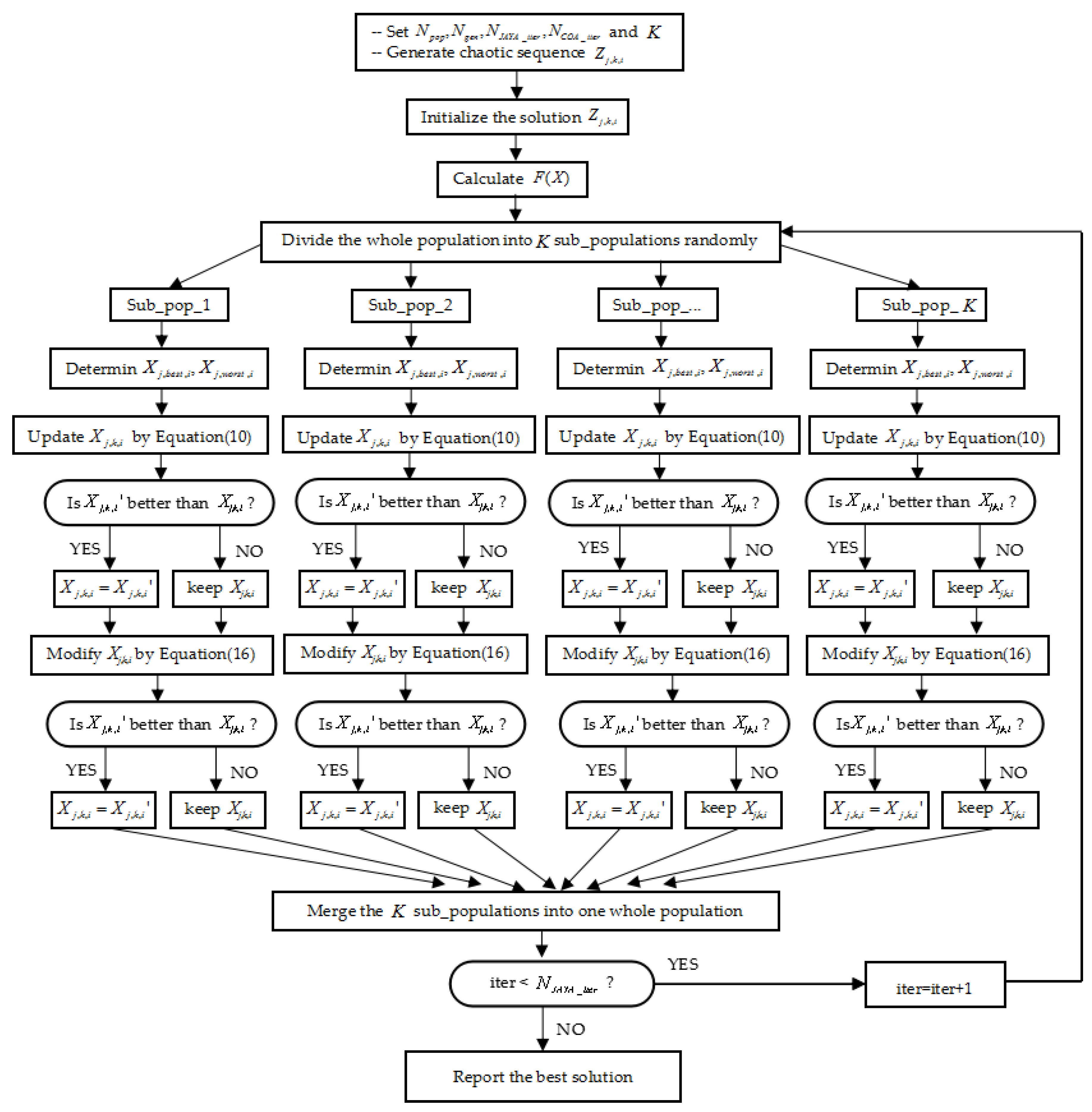
In this section, Multi-population based optimization method (MP) is combined with CJAYA algorithm to form the proposed MP-CJAYA algorithm. Figure 1 presents the flowchart of the proposed MP-CJAYA algorithm, the pseudo code of the proposed MP-CJAYA is described in Algorithm 1. The whole steps of MP-CJAYA to solve ELD problem is described as follows, the symbol denotes a newly added step compared with CJAYA:
Step 1: Set parameters. Common parameters of MP-CJAYA are initialized in this step. The population size (), the maximum iteration number (), the total number of generators () and the maximum COA iteration number () are as the same as basic JAYA and CJAYA. However, another important parameter () is introduced which represents the divided number of sub-populations, so the population size of the sub-populations () is:
Set the iteration counter as iter.
Step 2: Generate chaotic sequence. As the same as Step 2 in Section 3.2.
Step 3: Initialize the solution. As the same as Step 3 in Section 3.2.
Step 4: Apply constraints. As the same as Step 3 in Section 3.1.
Step 5: Evaluate the solution. As the same as Step 4 in Section 3.1.
Step 6: Divide the population. The entire population is divided into sub-populations with population size of by Equation (17). It is noted that the solutions in the whole population are randomly assigned to a sub-population, each sub-population is arranged to explore a different area of the whole search space.
The following steps are performed on each sub-population:
Step 7: Determine the best and worst. As the same as Step 5 in Section 3.1.
Step 8: Generate new solution. As the same as Step 6 in Section 3.1.
Step 9: Apply constraints. As the same as Step 7 in Section 3.1.
Step 10: Evaluate the new solution. As the same as Step 8 in Section 3.1.
Step 11: Compare. As the same as Step 9 in Section 3.1.
Step 12: Apply COA. As the same as Step 11 in Section 3.2.
Step 13: Check the stopping condition. If the current iteration number reaches , stop the loop and report the best solution; otherwise follow the next step and set .
Step 14: Merge the sub-populations. All the sub-populations are merged together to form one population, then for re-divide the population go to Step 6.
| Algorithm 1 Pseudo code of the MP-CJAYA Algorithm |
| Begin |
| Initialize ,,, and ; |
| Generate initial solution by chaotic sequence; |
| Calculate objective function value ; |
| Set |
| Whiledo |
| Divide the whole population into sub-populations by Equation (17) randomly |
| Fordo |
| Confirm and within |
| Fordo |
| Generate new solution by Equation (10) |
| End for |
| If is better than then |
| Else |
| Keep the old value |
| End if |
| Fordo |
| Generate new solution by Equation (16) |
| If is better than then |
| Else |
| Keep the old value |
| End if |
| End for |
| End for |
| Merge the sub-populations () into |
| End while |
4. Experimental Results and Analysis
In this section, the basic JAYA, the compared CJAYA and the proposed MP-CJAYA algorithms are applied on the following ELD cases to test their performances:
- Case I.
- 3-units system for load demand of 850 MW.
- Case II.
- 13-units system for load demand of 2520 MW.
- Case III.
- 40-units system for load demand of 10500 MW.
- Case IV.
- 6-units system for load demand of 1263 MW.
- Case V.
- 15-units system for load demand of 2630 MW.
Since for meta-heuristic algorithms, parameter setting is critical for the quality of their performances, so the parameters used in the cases above are all listed below. All the cases are run in MATLAB 2016 under windows 7 on Intel(R) Core(TM) i5-6500 CPU 3.20 GHz, with 8 GB RAM.
4.1. Case I: 3-Units System for Load Demand of 850 MW
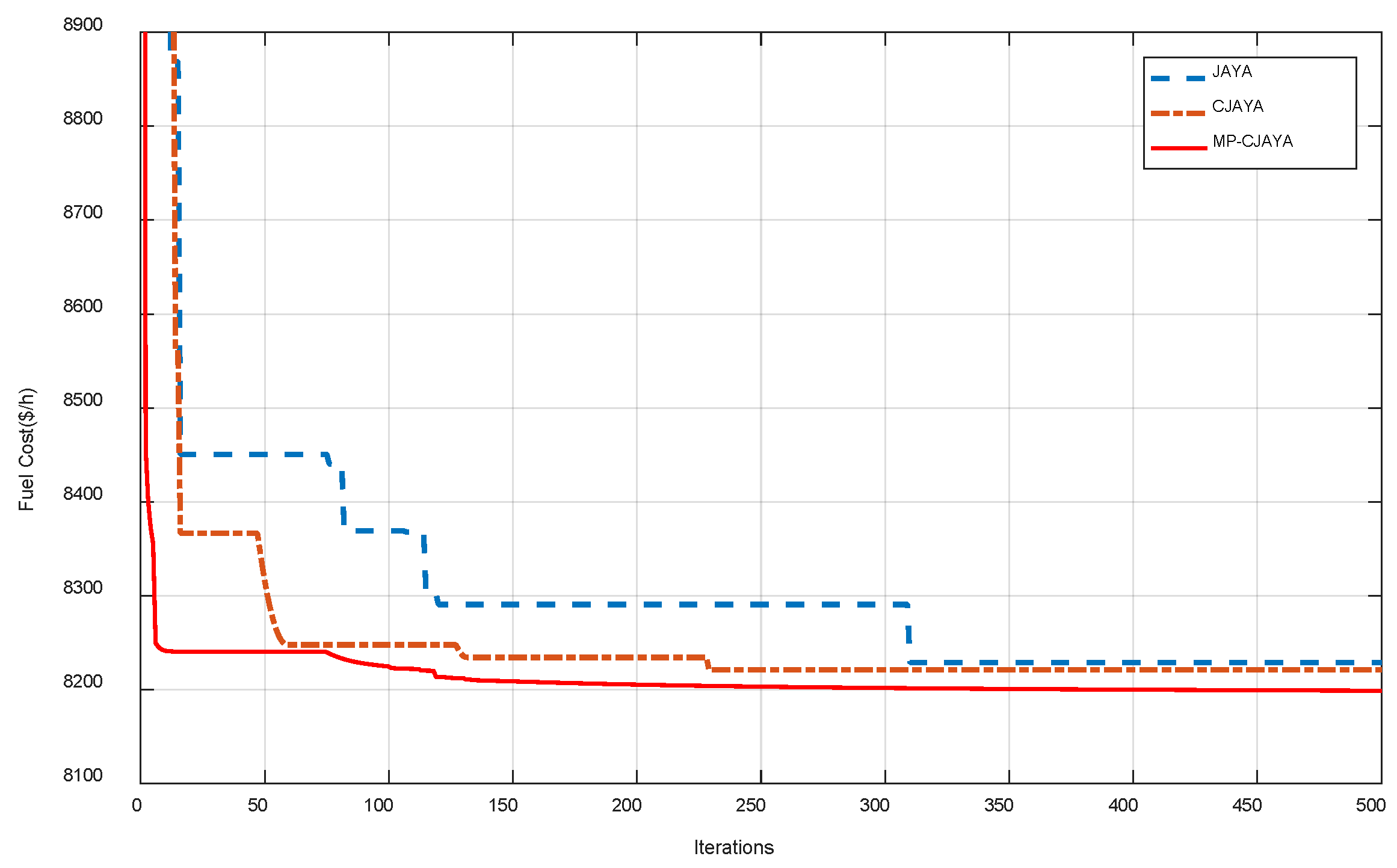
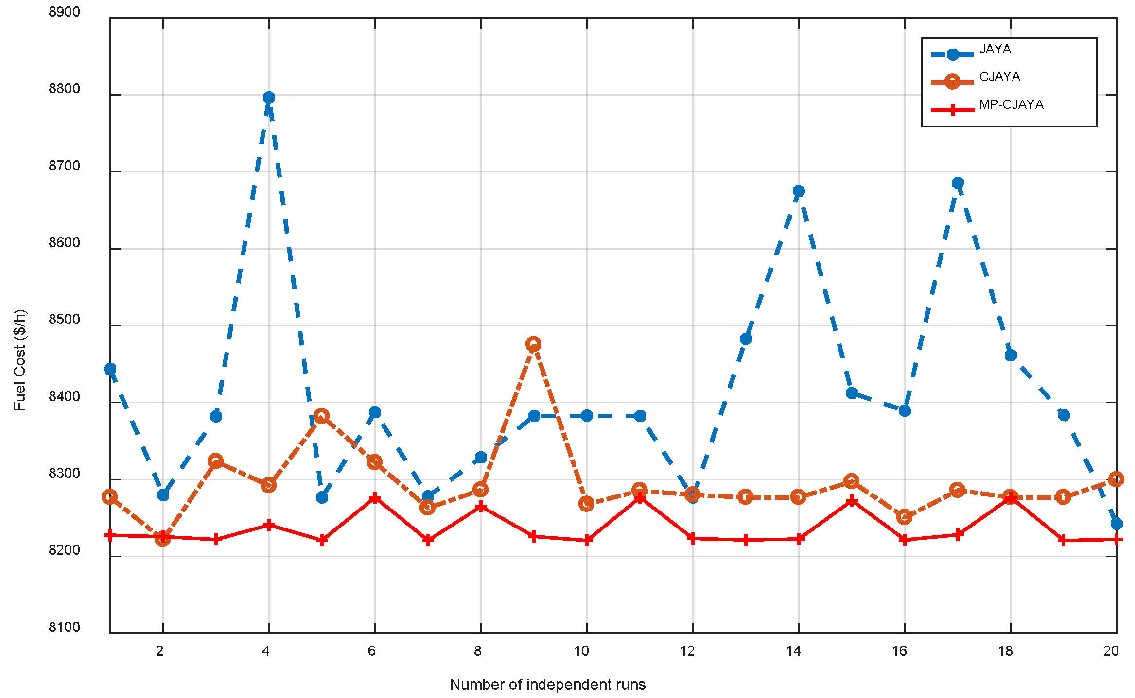
All detailed data are provided in [44]. The common parameters and constraint conditions are given in Table 1. The cost value of and obtained by JAYA, CJAYA and MP-CJAYA are compared with GA [45], EP [45], EP-SQP [45], PSO [45], PSO-SQP [45], CPSO [46] and CPSO-SQP [46] in Table 2. The best cost are highlighted in bold font. Obviously, all the compared algorithms give the same best cost of 8234.07 $/h, except for GA who did not meet the load demand. However, JAYA, CJAYA and MP-CJAYA are able to give continuously decreasing values of Fbest and MP-CJAYA achieves the minimum value of 8223.29 $/h, as well as the minimum value of Fmean which is 8232.06 $/h. To observe the cost convergence characteristics more visually, Figure 2 depicts one randomly chosen convergence curve from 20 times of independent runs (Nruns). We can see that JAYA has been trapped into local optimum at about 320 iterations and CJAYA has also settled down at around 230 iterations, but MP-CJAYA has showed extraordinary fast convergence ability at the beginning of 10 iterations and reached global optimum at approximately 200 iterations. It reveals that MP-CJAYA has faster convergence rate compared with JAYA and CJAYA due to its strong searching ability. Figure 3 shows the distribution outlines of Fbest at each independent run time. In case of MP-CJAYA, the value of Fbest after each run remains more or less steady, whereas in CJAYA the value of Fbest varies much more than MP-CJAYA, while JAYA shows the worst stability of Fbest with maximum cost as much as 8800 $/h. This indicates that MP-CJAYA is more consistent and robust than CJAYA and JAYA.
4.2. Case II: 13-Units System for Load Demand of 2520 MW
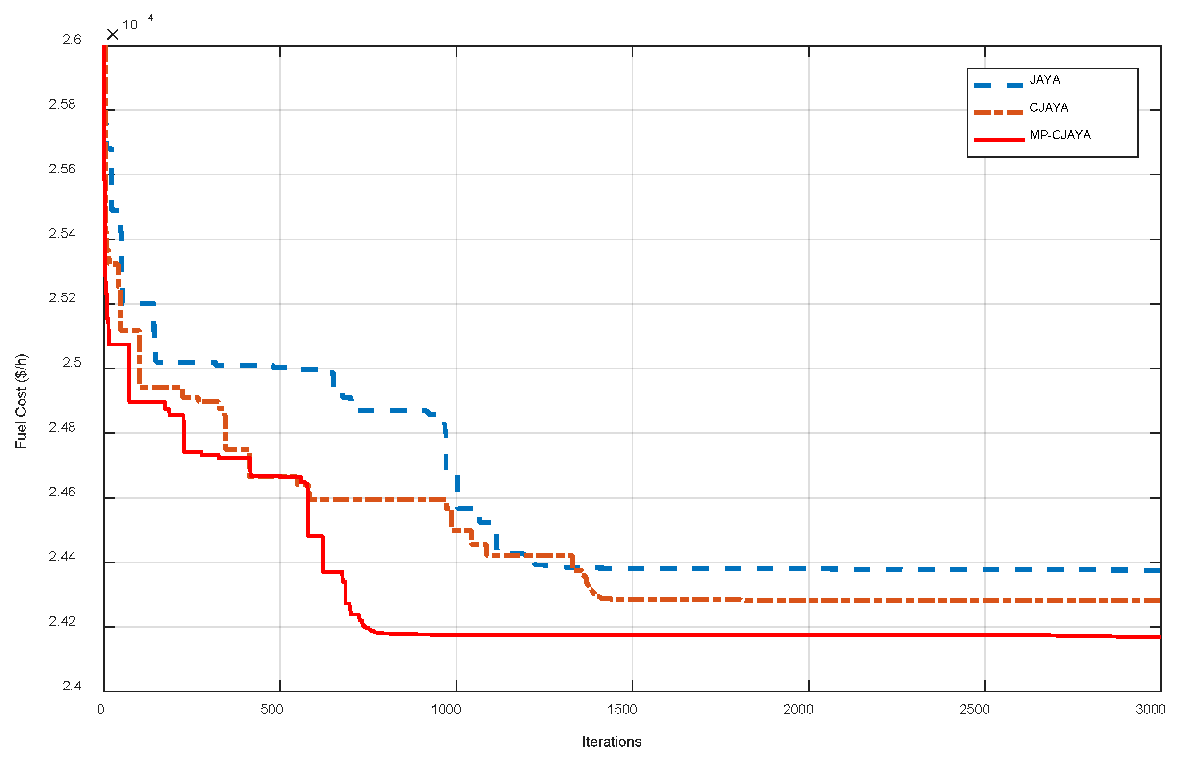
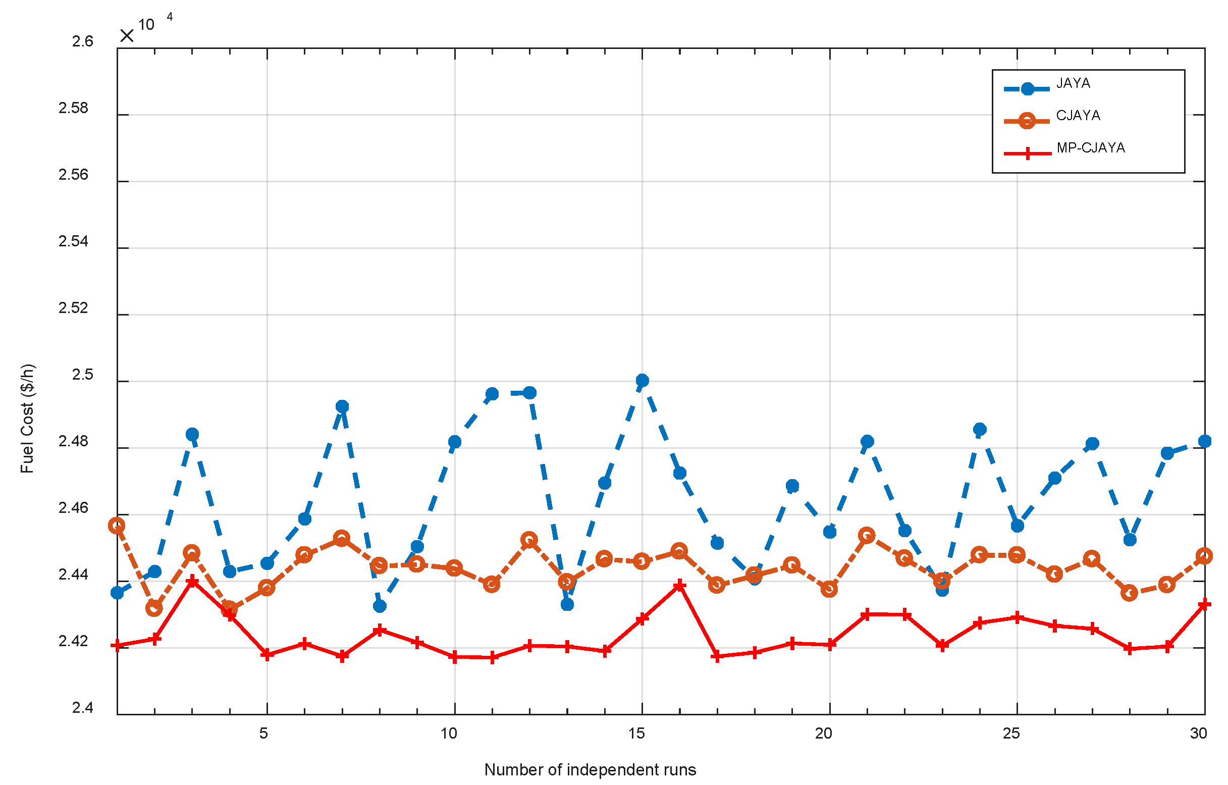
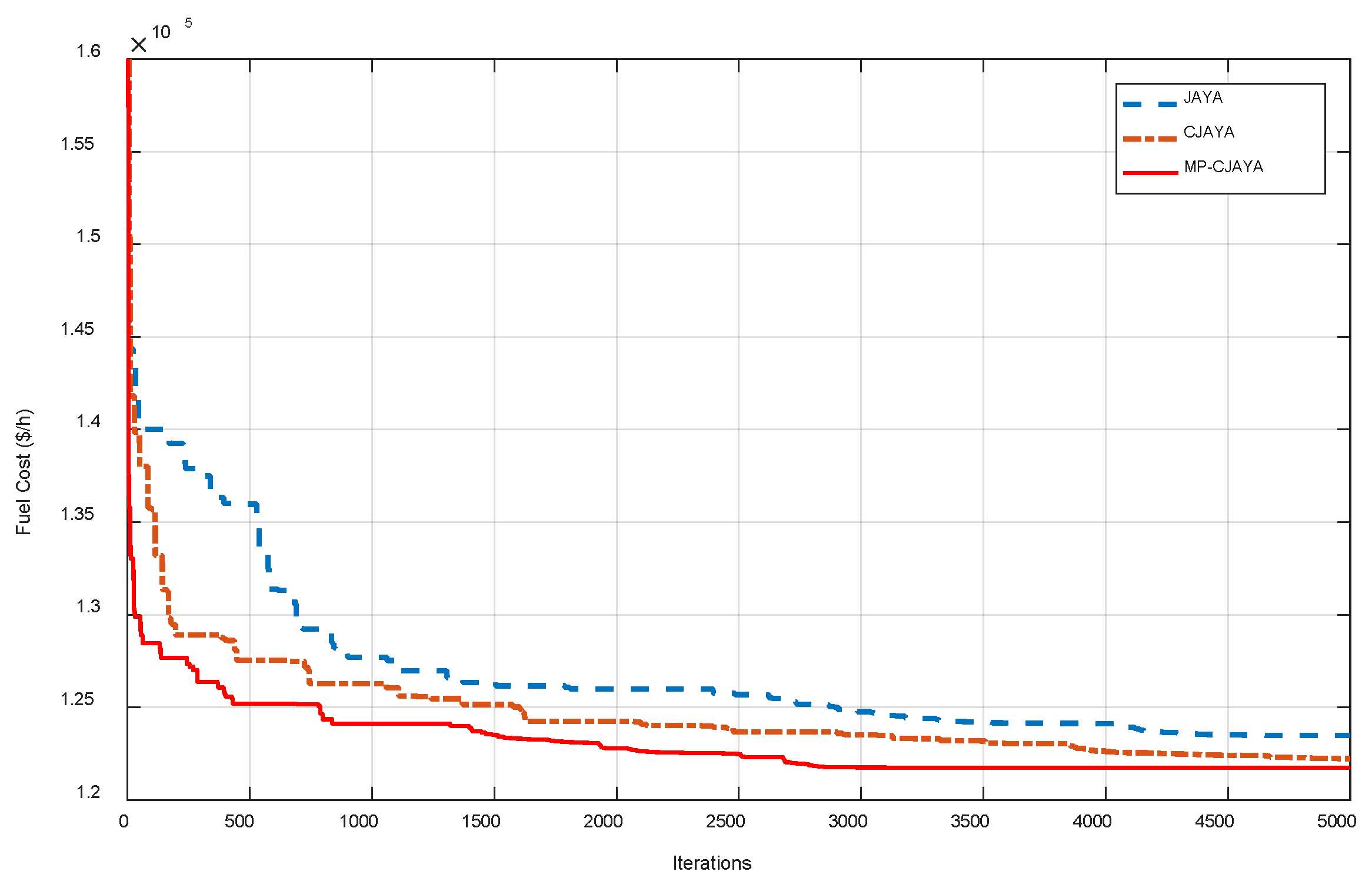
As the same as case I, all detailed data are provided in [44]. Since the increasing number of generators causes more non-linearity and complexity, Npop, NJAYA_iter and Nruns have all increased in this case, which are given in Table 1. The best individual of dispatched outputs obtained by different methods including GA [47], SA [47], HSS [47], EP-SQP [45], PSO-SQP [45], CPSO [46], CPSO-SQP [46], JAYA, CJAYA and MP-CJAYA are reported in Table 3. The best cost are highlighted in bold font. It is observed that the minimum value of Fmean and Fbest are both achieved by MP-CJAYA, which is 24,228.1331 $/h and 24,175.5444 $/h respectively. In Figure 4 the convergence curve of MP-CJAYA is compared with JAYA and CJAYA, it can be observed that JAYA has been trapped into a local optimum in about 1300 iterations, while CJAYA has the same problem at around 1500 iterations. However, the proposed MP-CJAYA has greatly accelerated the convergence rate and reached the best value within only 750 iterations. Figure 5 is the distribution outlines of Fbest at each run time. Once again, it can be easily compared that MP-CJAYA shows the most robust characteristic among the three versions of JAYA due to most of its independent runs have achieved getting close to the best individual. All the comparisons above real that MP-CJAYA has greatly improved the best cost, the mean cost, the convergence rate and the consistency of the solution.
4.3. Case III: 40-Units System for Load Demand of 10,500 MW
In order to investigate the effectiveness of MP-CJAYA for larger scale power system, it is further evaluated by 40 generating units with load demand of 10,500 MW, which is the largest system of ELD problem considering the valve-point effect in the available literature. Considering the increased number of generators and the much more complex solution space, Npop, NJAYA_iter, NCOA_iter, Nsub_pop and Nruns have all increased, as shown in Table 1. The results comparison from methods PSO-LRS [48], NPSO [48], NPSO-LRS [48], SPSO [49], PC-PSO [49], SOH-PSO [49], JAYA, CJAYA and MP-CJAYA are shown in Table 4. The minimum value of Fmean and Fbest are highlighted in bold font. It is observed that MP-CJAYA has achieved the minimum value of Fbest among all the values by above-mentioned methods, which is 121,480.10 $/h. What’s more, the minimum value of Fmean is also achieved by MP-CJAYA, which is 121,861.08 $/h. In Figure 6 the convergence curve of MP-CJAYA is compared with JAYA and CJAYA, it can easily be observed that CJAYA performs better than JAYA due to the local searching ability provided by COA, while MP-CJAYA shows superiority over CJAYA due to the extra searching diversification provided by MP method.
Figure 7 is the distribution outlines of Fbest within 50 times of independent runs. Once again, it can be observed that MP-CJAYA shows the most robust characteristic among the three versions of JAYA because most of the Fbest value keeps steady and very close to the best individual. The comparisons have verified that MP-CJAYA get better results than all of the other algorithms in best cost, mean cost, convergence rate and consistency when dealing with larger scale power system.
4.4. Case IV: 6-Units System for Load Demand of 1263 MW
In this case, the three versions of JAYA are applied to 6-units system with constraints of ramp rate limit, prohibited operating zones (POZs) and transmission loss (), as shown in Table 1. The generator data and B-coefficients have been taken from [50]. For every generator it has two , this problem causes challenging complexity to find the global optima because of increasing number of non-convex decision spaces.
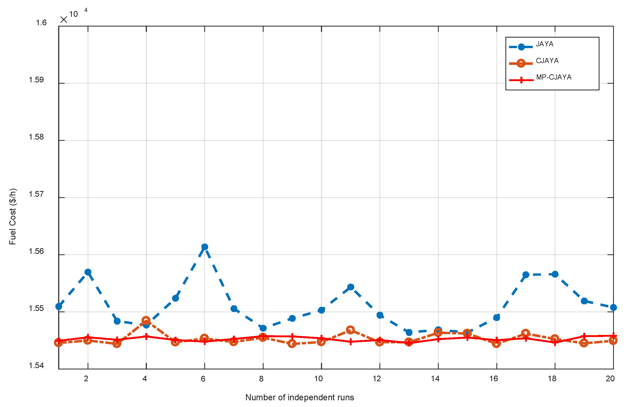
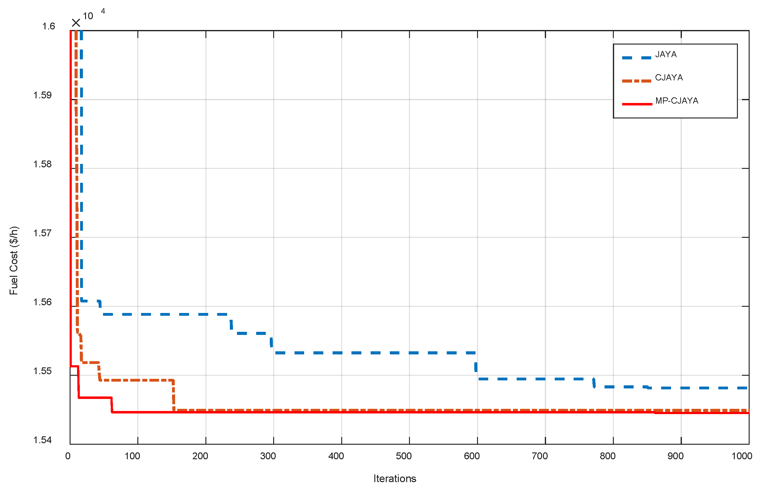
The best individual achieved by MP-CJAYA, as well the other algorithms such as SA [51], GA [51], TS [51], PSO [51], MTS [51], PSO-LRS [48], NPSO [48], NPSO-LRS [48], JAYA and CJAYA have been recorded in Table 5. It can be observed that MP-CJAYA provides the lowest Fbest among all the methods as 15,446.17 $/h, while CJAYA and JAYA provide the second and third lowest Fbest as 15,446.71 $/h and 15,447.09 $/h. Furthermore, the best cost Fbest, the worst cost Fworst and the mean cost Fmean of the three version of JAYA algorithms are also compared with those above-mentioned methods and summarized in Table 6. It can be found that MP-CJAYA is superior to all the other compared methods and achieves the minimum value of Fbest, Fworst and Fmean at the same time, which are highlighted in bold font. Figure 8 is the distribution outlines of Fbes, it can be noticed that MP-CJAYA shows the most robust characteristic and the value keeps almost steady within 20 independent runs, which has greatly surpassed JAYA and a little surpassed CJAYA. One randomly chosen convergence curve of fuel cost is shown in Figure 9, from which we can see that MP-CJAYA is extraordinary fast in convergence rate and approaches global optimum within only about 60 iterations. It all demonstrates that MP-CJAYA has the strongest capabilities of handling ELD problems with different constraint conditions.
4.5. Case V: 15-Units System for Load Demand of 2630 MW
In the last case, the three versions of JAYA are applied to a larger 15-units system with the same constraints as in case 4, the system data and B-coefficients have been taken from [50]. There are 4 generators having . Generators 2, 5 and 6 have three and generator 12 has two . Considering that these result in non-convex decision spaces consisting of 192 convex sub-spaces, the value of , , , and are all increased compared to Case IV to cope with the challenges.
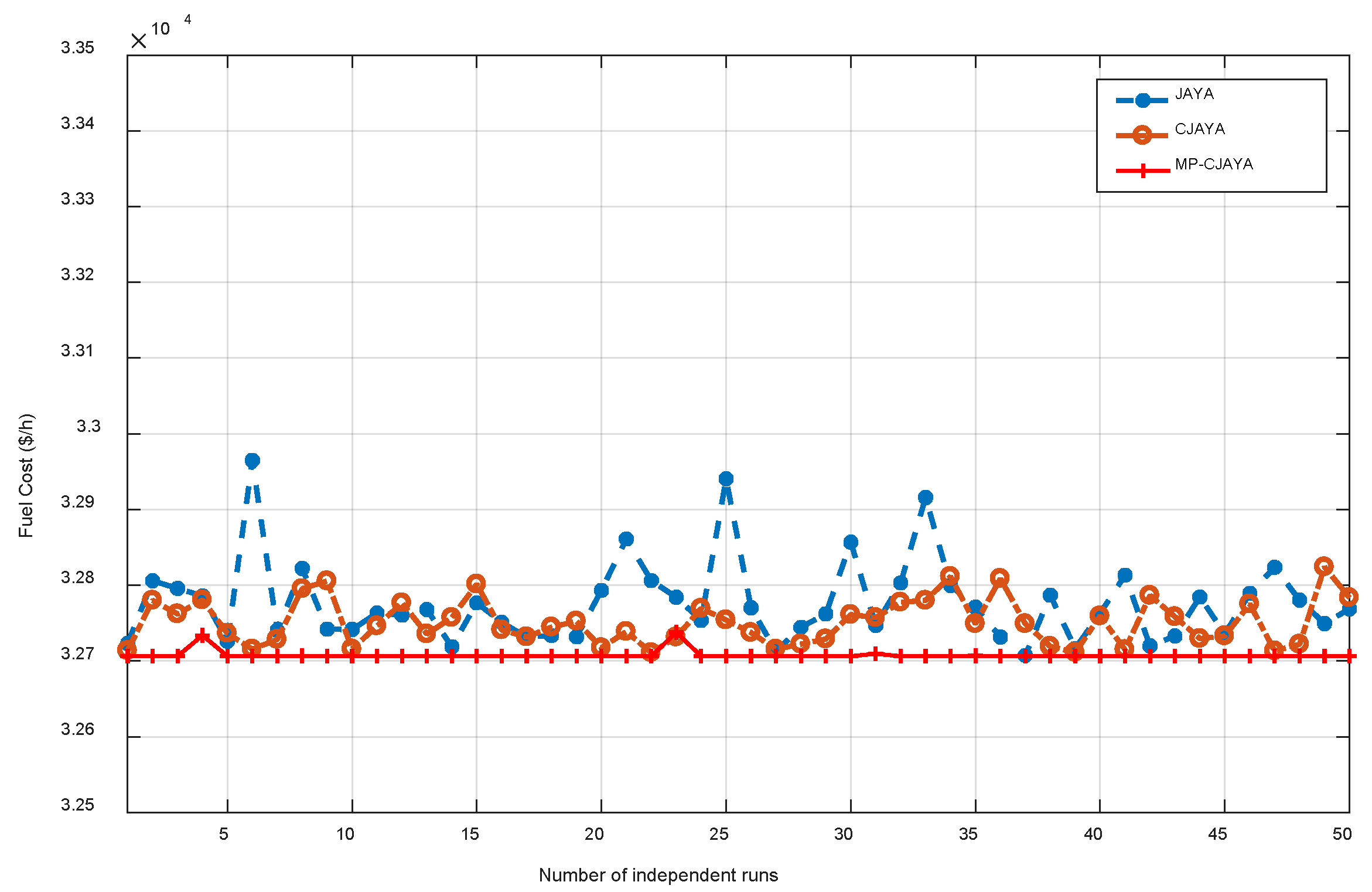
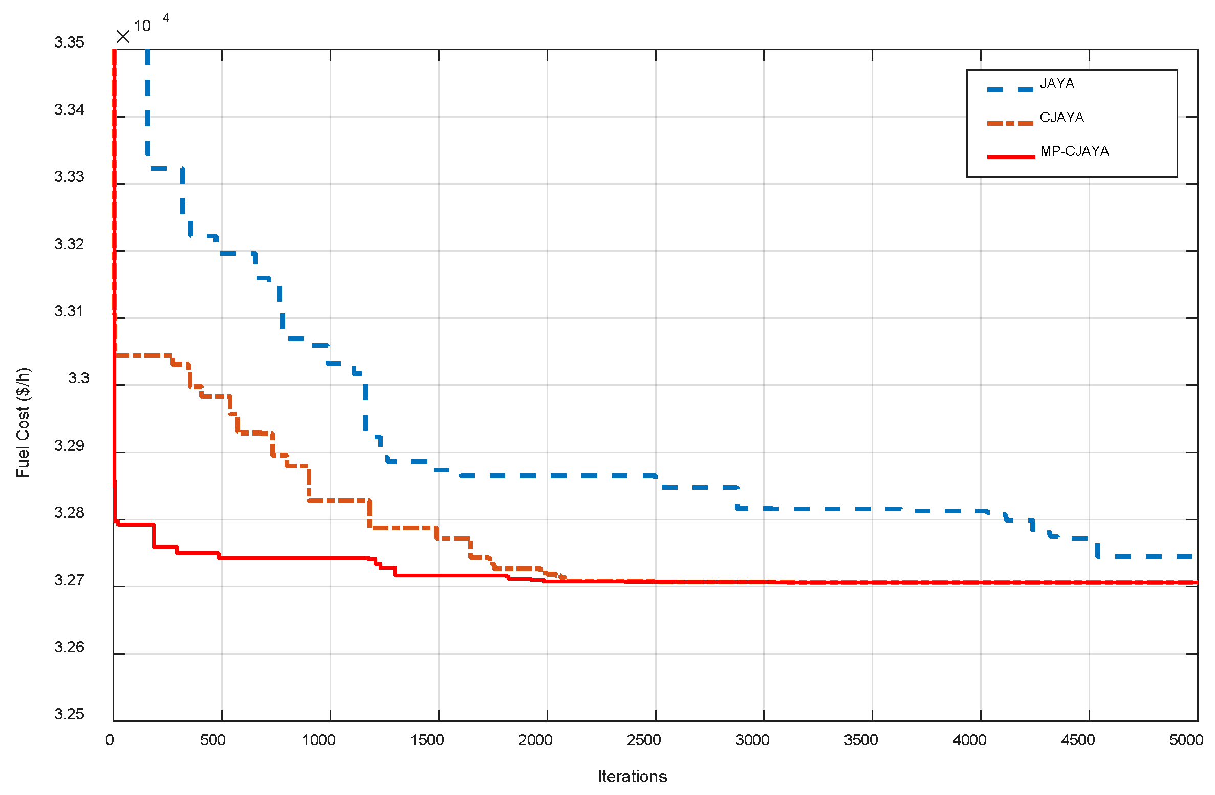
The best outputs from JAYA, CJAYA, MP-CJAYA and other algorithms including SA [51], GA [51], TS [51], PSO [51], MTS [51], TSA [52], DSPSO-TSA [52] and AIS [53] are summarized in Table 7. From the table we can observe that DSPSO-TSA has provided lower than JAYA, but it is not as lowest as CJAYA and MP-CJAYA, which obtains 32,710.0768 $/h and 32,706.5158 $/h respectively and ranks the second and first best value among all the algorithms. Furthermore, in addition to the best cost , the worst cost and the mean cost of the three version of JAYA algorithms are also compared with those above-mentioned methods in Table 8. It can be found that MP-CJAYA achieves the minimum value of , and at the same time, which are highlighted in bold font. Figure 10 is the distribution outlines of , we can notice that MP-CJAYA exhibits the best consistency in achieving minimum within 50 independent runs. One randomly chosen convergence curve is shown in Figure 11, from which we can see that CJAYA has improved the convergence rate and accuracy of basic JAYA, while MP-CJAYA has made further improvements of CJAYA in the rate of approaching the lowest cost. From the analysis above, it can be concluded that MP-CJAYA has the strongest capabilities of handling larger size of ELD problems with different constraint conditions.
5. Discussion and Conclusions
A novel multi-population based chaotic JAYA algorithm (MP-CJAYA) is proposed in this paper. By introducing the MP method and chaotic map to the basic JAYA algorithm, both the global exploration capability and the local searching capability have been greatly improved. MP-CJAYA is employed in five typical ELD cases to compare the performances with other well-established algorithms in terms of best solutions, convergence rate and robustness. The results have proved that MP-CJAYA algorithm has outstanding superiority to all the other compared algorithms in all cases.
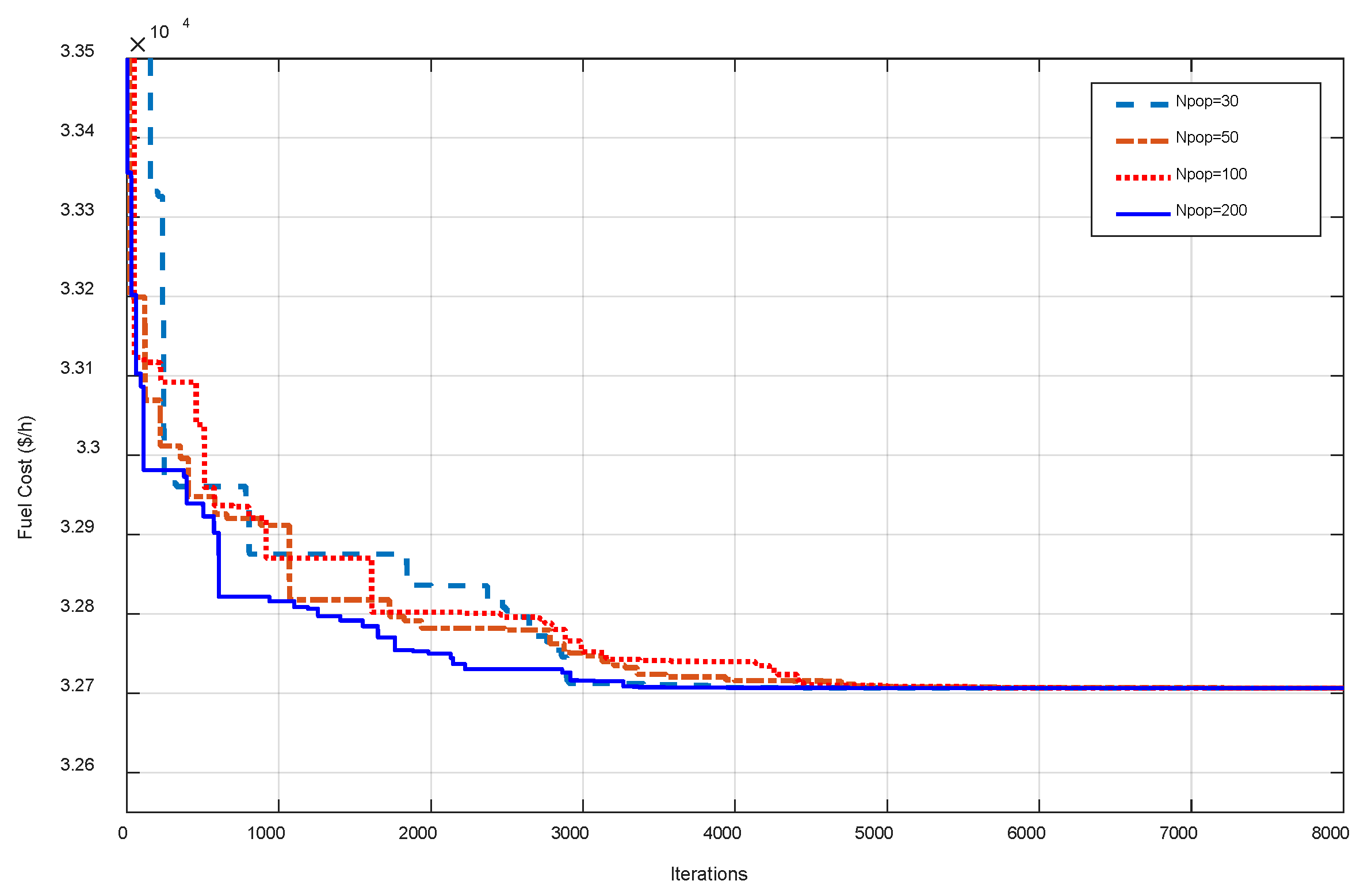
It is noteworthy that for most of the meta-heuristic algorithms, parameter setting is critical for the quality of their results. But for MP-CJAYA, it does not require for specific algorithm parameters except for common parameters. What’s more, it is observed that the common parameter population size (Npop) does not affect the performance of its final optimal solution significantly, as shown in Figure 12. With increased Npop of 30, 50, 100 and 200 under the same circumstances, a slightly steady improvement of the convergence rate can be observed at initial part of the iteration. However, after about 5000 iterations, the differences among those curves become difficult to be observed and they all have reached the same best solution, which has proved that MP-CJAYA algorithm is not highly dependent on the common parameter Npop.
As a newly proposed meta-heuristic algorithm, even though MP-CJAYA has gained the most outstanding superiority in this paper, it still has not been used for solving other optimization issues, except for the ELD problem. Hence, authors are planning to apply it to different kinds of optimization issues in the future to broaden its applications, such as multiple fuel options, micro grid power dispatch problems and multi-objective scheduling optimization problems.
Author Contributions
Conceptualization, J.Y., C.-H.K. and S.-B.R.; Data curation, J.Y.; Formal analysis, J.Y., A.W. and T.K.; Investigation, J.Y., C.-H.K., A.W. and T.K.; Methodology, J.Y. and S.-B.R.; Software, J.Y. and C.-H.K.; Supervision, S.-B.R.; Writing—Original Draft, J.Y.; Writing—Review & Editing, A.W. and T.K.
Funding
This research received no external funding.
Acknowledgments
Authors would like to thank Yeungnam University for all the supports in terms of fellowship to Jiangtao Yu.
Conflicts of Interest
The authors declare no conflict of interest.
References
- Narimani, MR.; Joo, J.-Y.; Crow, M.L. Dynamic Economic Dispatch with Demand Side Management of Individual Residential Loads. In Proceedings of the 2015 North American Power Symposium (NAPS), Charlotte, NC, USA, 4–6 October 2015. [Google Scholar]
- Dodu, J.C.; Martin, P.; Merlin, A.; Pouget, J. An optimal formulation and solution of short-range operating problems for a power system with flow constraints. Proc. IEEE 1972, 60, 54–63. [Google Scholar] [CrossRef]
- Chen, C.L.; Wang, S.C. Branch-and-bound scheduling for thermal generating units. IEEE Trans. Energy Convers. 1993, 8, 184–189. [Google Scholar] [CrossRef]
- Jubril, A.; Olaniyan, O.; Komolafe, O.; Ogunbona, P.O. Economic-emission dispatch problem: A semi-definite programming approach. Appl. Energy 2014, 134, 446–455. [Google Scholar] [CrossRef]
- Papageorgiou, L.G.; Fraga, E.S. A mixed integer quadratic programming formulation for the economic dispatch of generators with prohibited operating zones. Electr. Power Syst. Res. 2007, 77, 1292–1296. [Google Scholar] [CrossRef] [Green Version]
- Liang, Z.X.; Glover, J.D. A zoom feature for a dynamic programming solution to economic dispatch including transmission losses. IEEE Trans. Power Syst. 1992, 7, 544–550. [Google Scholar] [CrossRef]
- El-Keib, A.A.; Ma, H.; Hart, J.L. Environmentally constrained economic dispatch using the Lagrangian relaxation method. IEEE Trans. Power Syst. 1994, 9, 1723–1729. [Google Scholar] [CrossRef]
- Farag, A.; Al-Baiyat, S.; Cheng, T. Economic load dispatch multiobjective optimization procedures using linear programming techniques. IEEE Trans. Power Syst. 1995, 10, 731–738. [Google Scholar] [CrossRef]
- Niknam, T. A new fuzzy adaptive hybrid particle swarm optimization algorithm for non-linear, non-smooth and non-convex economic dispatch problem. Appl. Energy 2010, 87, 327–339. [Google Scholar] [CrossRef]
- Chiang, C.L. Improved genetic algorithm for power economic dispatch of units with valve-point effects and multiple fuels. IEEE Trans. Power Syst. 2005, 20, 1690–1699. [Google Scholar] [CrossRef]
- Park, J.B.; Lee, K.S.; Shin, J.R.; Lee, K.Y. A particle swarm optimization for economic dispatch with non-smooth cost functions. IEEE Trans. Power Syst. 2005, 20, 34–42. [Google Scholar] [CrossRef]
- Lin, W.M.; Cheng, F.S.; Tsay, M.T. An improved tabu search for economic dispatch with multiple minima. IEEE Trans. Power Syst. 2002, 17, 108–112. [Google Scholar] [CrossRef]
- Secui, D.C. A new modified artificial bee colony algorithm for the economic dispatch problem. Energy Convers. Manag. 2015, 89, 43–62. [Google Scholar] [CrossRef]
- Yang, X.S.; Sadat Hosseini, S.S.; Gandomi, A.H. Firefly algorithm for solving non-convex economic dispatch problems with valve loading effect. Appl. Soft Comput. 2012, 12, 1180–1186. [Google Scholar] [CrossRef]
- Dos Santos Coelho, L.; Mariani, V.C. An improved harmony search algorithm for power economic load dispatch. Energy Convers. Manag. 2009, 50, 2522–2526. [Google Scholar] [CrossRef]
- He, X.Z.; Rao, Y.Q.; Huang, J.D. A novel algorithm for economic load dispatch of power systems. Neurocomputing 2016, 171, 1454–1461. [Google Scholar] [CrossRef]
- Niknam, T.; Mojarrad, H.D.; Meymand, H.Z. A novel hybrid particle swarm optimization for economic dispatch with valve-point loading effects. Energy Convers. Manag. 2011, 52, 1800–1809. [Google Scholar] [CrossRef]
- Wang, L.; Li, L.P. An effective differential harmony search algorithm for the solving non-convex economic load dispatch problems. Int. J. Electr. Power Energy Syst. 2013, 44, 832–843. [Google Scholar] [CrossRef]
- Alsumait, J.S.; Sykulski, J.; Al-Othman, A. A hybrid GA-PS-SQP method to solve power system valve-point economic dispatch problems. Appl. Energy 2010, 87, 1773–1781. [Google Scholar] [CrossRef]
- Mahdi, F.P.; Vasant, P. Quantum particle swarm optimization for economic dispatch problem using cubic function considering power loss constraint. IEEE Trans. Power Syst. 2002, 17, 108–112. [Google Scholar]
- Rao, R.V. Jaya: A simple and new optimization algorithm for solving constrained and unconstrained optimization problems. Int. J. Ind. Eng. Comput. 2016, 7, 19–34. [Google Scholar]
- Warid, W.; Hizam, H.; Mariun, N.; Abdul-Wahab, N.I. Optimal power flow using the JAYA algorithm. Energies 2016, 9, 678. [Google Scholar] [CrossRef]
- Rao, R.V.; Saroj, A. Multi-objective design optimization of heat exchangers using elitist-JAYA algorithm. Energy Syst. 2018, 9, 305–341. [Google Scholar] [CrossRef]
- Yu, K.J.; Liang, J.J.; Qu, B.Y. Parameters identification of photovoltaic models using an improved JAYA optimization algorithm. Energy Convers. Manag. 2017, 150, 742–753. [Google Scholar] [CrossRef]
- Rao, R.V.; More, K. Design optimization and analysis of selected thermal devices using self-adaptive JAYA algorithm. Energy Convers. Manag. 2017, 140, 24–35. [Google Scholar] [CrossRef]
- Huang, C.; Wang, L.; Yeung, R.S. A prediction model guided JAYA algorithm for the PV system maximum power point tracking. IEEE Trans. Sustain. Energy 2018, 9, 45–55. [Google Scholar] [CrossRef]
- Rao, R.V.; Waghmare, G. A new optimization algorithm for solving complex constrained design optimization problems. Eng. Opt. 2017, 49, 60–83. [Google Scholar] [CrossRef]
- Rao, R.V.; Rai, D.P.; Balic, J. A multi-objective algorithm for optimization of modern machining processes. Eng. Appl. Artif. Intell. 2017, 61, 103–125. [Google Scholar] [CrossRef]
- Mishra, S.; Ray, P.K. Power quality improvement using photovoltaic fed DSTATCOM based on JAYA optimization. IEEE Trans. Sustain. Energy 2016, 7, 1672–1680. [Google Scholar] [CrossRef]
- Nguyen, T.T.; Yang, S.; Branke, J. Evolutionary dynamic optimization: a survey of the state of the art. Swarm Evol. Comput. 2012, 6, 1–24. [Google Scholar] [CrossRef]
- Cruz, C.; González, J.R.; Pelta, D.A. Optimization in dynamic environments: a survey on problems methods and measures. Soft Comput. 2011, 15, 1427–1448. [Google Scholar] [CrossRef]
- Branke, J.; Kaußler, T.; Schmidt, C.; Schmeck, H. A multi-population approach to dynamic optimization problems. Evol. Des. Manuf. 2000, 299–309. [Google Scholar] [CrossRef]
- Turky, A.M.; Abdullah, S. A multi-population electromagnetic algorithm for dynamic optimization problems. Appl. Soft Comput. 2014, 22, 474–482. [Google Scholar] [CrossRef]
- Turky, A.M.; Abdullah, S. A multi-population harmony search algorithm with external archive for dynamic optimization problems. Inf. Sci. 2014, 272, 84–95. [Google Scholar] [CrossRef]
- Nseef, S.K.; Abdullah, S.; Turky, A.; Kendall, G. An adaptive multi-population artificial bee colony algorithm for dynamic optimization problems. Knowl. Based Syst. 2016, 104, 14–23. [Google Scholar] [CrossRef]
- Li, C.; Nguyen, T.T.; Yang, M.; Yang, S.; Zeng, S. Multi-population methods in un-constrained continuous dynamic environments: the challenges. Inf. Sci. 2015, 296, 95–118. [Google Scholar] [CrossRef]
- Caponetto, R.; Fortuna, L.; Fazzino, S.; Gabriella, M. Chaotic sequences to improve the performance of evolutionary algorithms. IEEE Trans. Evol. Comput. 2003, 7, 289–304. [Google Scholar] [CrossRef]
- Li, Y.; Wen, Q.; Li, L.; Peng, H. Hybrid chaotic ant swarm optimization. Chaos Solitons Fractals 2009, 42, 880–889. [Google Scholar] [CrossRef]
- Alatas, B. Chaotic harmony search algorithms. Appl. Math. Comput. 2010, 216, 2687–2699. [Google Scholar] [CrossRef]
- Chuang, L.-Y.; Tsai, S.-W.; Yang, C.-H. Chaotic catfish particle swarm optimization for solving global numerical optimization problems. Appl. Math. Comput. 2011, 217, 6900–6916. [Google Scholar] [CrossRef]
- Dos Santos Coelho, L.; Mariani, V.C. Firefly algorithm approach based on chaotic Tinkerbell map applied to multivariable PID controller tuning. Comput. Math. Appl. 2012, 64, 2371–2382. [Google Scholar] [CrossRef]
- Narimani, M.R.; Joo, J.-Y.; Crow, M. Multi-objective dynamic economic dispatch with demand side management of residential loads and electric vehicles. Energies 2017, 10, 624. [Google Scholar] [CrossRef]
- Heidari-Bateni, G.; McGillem, C.D. A chaotic direct-sequence spread-spectrum communication system. IEEE Trans. Commun. 1994, 42, 1524–1527. [Google Scholar] [CrossRef]
- Sinha, N.; Chakrabarti, R.; Chattopadhyay, P. Evolutionary programming techniques for economic load dispatch. IEEE Trans. Evol. Comput. 2003, 7, 83–94. [Google Scholar] [CrossRef]
- Victoire, T.A.A.; Jeyakumar, A.E. Hybrid PSO–SQP for economic dispatch with valve-point effect. Electr. Power Syst. Res. 2004, 71, 51–59. [Google Scholar] [CrossRef]
- Cai, J.; Li, Q. A hybrid CPSO–SQP method for economic dispatch considering the valve-point effects. Energy Convers. Manag. 2012, 53, 175–181. [Google Scholar] [CrossRef]
- Bhagwan Das, D.; Patvardhan, C. Solution of Economic Load Dispatch using real coded Hybrid Stochastic Search. Int. J. Electr. Power Energy Syst. 1999, 21, 165–170. [Google Scholar] [CrossRef]
- Selvakumar, I.; Thanushkodi, K. A new particle swarm optimization solution to nonconvex economic dispatch problems. Electr. Power Syst. Res. 2007, 22, 42–51. [Google Scholar] [CrossRef]
- Chaturvedi, K.T.; Pandit, M. Self-Organizing Hierarchical Particle Swarm Optimization for Nonconvex Economic Dispatch. IEEE Trans. Power Syst. 2008, 23, 1079–1087. [Google Scholar] [CrossRef]
- Gaing, Z.L. Particle swarm optimization to solving the economic dispatch considering the generator constraints. IEEE Trans. Power Syst. 2003, 18, 1187–1195. [Google Scholar] [CrossRef] [Green Version]
- Pothiya, S.; Ngamroo, I.; Kongprawechnon, W. Application of multiple tabu search algorithm to solve dynamic economic dispatch considering generator constraints. Energy Convers. Manag. 2008, 49, 506–516. [Google Scholar] [CrossRef]
- Khamsawang, S.; Jiriwibhakorn, S. DSPSO–TSA for economic dispatch problem with nonsmooth and noncontinuous cost functions. Energy Convers. Manag. 2010, 51, 365–375. [Google Scholar] [CrossRef]
- Panigrahi, B.K.; Yadav, S.R.; Agrawal, S.; Tiwari, M.K. A clonal algorithm to solve economic load dispatch. Electr. Power Syst. Res. 2007, 77, 1381–1389. [Google Scholar] [CrossRef]
Figure 1.
Flow chart of the MP-CJAYA Algorithm.

Figure 2.
Fuel cost convergence characteristic of 3-units system ( = 850 MW).

Figure 3.
Fuel cost for 20 independent runs of 3-units system ( = 850 MW).

Figure 4.
Fuel cost convergence characteristic of 13-units system ( = 2520 MW).

Figure 5.
Fuel cost for 30 independent runs of 13-units system ( = 2520 MW).

Figure 6.
Fuel cost convergence characteristic of 40-units system ( = 10500 MW).

Figure 7.
Fuel cost for 50 independent runs of 40-units system ( = 10,500 MW).

Figure 8.
Fuel cost for 20 independent runs of 6-units system ( = 1263 MW).

Figure 9.
Fuel cost convergence characteristic of 6-units system ( = 1263 MW).

Figure 10.
Fuel cost for 50 independent runs of 15-units system ( = 2630 MW).

Figure 11.
Fuel cost convergence characteristic of 15-units system ( = 2630 MW).

Figure 12.
Convergence characteristics of MP-CJAYA with varying population sizes for case V.


Table 1.
Parameters and constraint conditions of the ELD cases.
| Case I | Case II | Case III | Case IV | Case V | |||||||||||
|---|---|---|---|---|---|---|---|---|---|---|---|---|---|---|---|
| JAYA | CJAYA | MP-CJAYA | JAYA | CJAYA | MP-CJAYA | JAYA | CJAYA | MP-CJAYA | JAYA | CJAYA | MP-CJAYA | JAYA | CJAYA | MP-CJAYA | |
| 20 | 20 | 20 | 50 | 50 | 50 | 100 | 100 | 100 | 20 | 20 | 20 | 100 | 100 | 100 | |
| 500 | 500 | 500 | 3000 | 3000 | 3000 | 5000 | 5000 | 5000 | 1000 | 1000 | 1000 | 5000 | 5000 | 5000 | |
| - | 20 | 20 | - | 20 | 20 | - | 30 | 30 | - | 20 | 20 | - | 30 | 30 | |
| - | - | 10 | - | - | 10 | - | - | 20 | - | - | 10 | - | - | 20 | |
| 20 | 20 | 20 | 30 | 30 | 30 | 50 | 50 | 50 | 20 | 20 | 20 | 50 | 50 | 50 | |
| Valve-point effect | ● | ● | ● | - | - | ||||||||||
| Ramp-rate limit | - | - | - | ● | ● | ||||||||||
| POZ | - | - | - | ● | ● | ||||||||||
| - | - | ● | ● | ||||||||||||
Table 2.
Best outputs for 3-units system ( = 850 MW).
| Unit | GA [45] | EP [45] | EP-SQP [45] | PSO [45] | PSO-SQP [45] | CPSO [46] | CPSO-SQP [46] | JAYA | CJAYA | MP-CJAYA |
|---|---|---|---|---|---|---|---|---|---|---|
| 1 | 398.700 | 300.264 | 300.267 | 300.268 | 300.267 | 300.267 | 300.266 | 350.3314 | 350.0254 | 350.2464 |
| 2 | 399.600 | 400.000 | 400.000 | 400.000 | 400.000 | 400.000 | 400.000 | 400.0000 | 400.0000 | 400.0000 |
| 3 | 50.100 | 149.736 | 149.733 | 149.732 | 149.733 | 149.733 | 149.734 | 99.6453 | 99.9511 | 99.7576 |
| (MW) | 848.400 | 850.000 | 850.000 | 850.000 | 850.000 | 850.000 | 850.000 | 849.977 | 849.977 | 850.004 |
| ($/h) | 8234.72 | 8234.16 | 8234.09 | 8234.72 | 8234.07 | NA | NA | 8382.10 | 8289.41 | 8232.06 |
| ($/h) | 8222.07 | 8234.07 | 8234.07 | 8234.07 | 8234.07 | 8234.07 | 8234.07 | 8230.23 | 8226.18 | 8223.29 |
NA indicates the cost value is not found.
Table 3.
Best outputs for 13-units system ( = 2520 MW).
| Unit | GA [47] | SA [47] | HSS [47] | EP-SQP [45] | PSO-SQP [45] | CPSO [46] | CPSO-SQP [46] | JAYA | CJAYA | MP-CJAYA |
|---|---|---|---|---|---|---|---|---|---|---|
| 1 | 628.32 | 668.40 | 628.23 | 628.3136 | 628.3205 | 628.32 | 628.31 | 628.3185 | 628.3185 | 628.3183 |
| 2 | 356.49 | 359.78 | 299.22 | 299.1715 | 299.0524 | 299.83 | 299.83 | 299.2009 | 299.1992 | 299.0170 |
| 3 | 359.43 | 358.20 | 299.17 | 299.0474 | 298.9681 | 299.17 | 299.16 | 306.9105 | 299.1993 | 299.1428 |
| 4 | 159.73 | 104.28 | 159.12 | 159.6399 | 159.4680 | 159.70 | 159.73 | 159.7339 | 159.7330 | 159.5714 |
| 5 | 109.86 | 60.36 | 159.95 | 159.6560 | 159.1429 | 159.64 | 159.73 | 159.7337 | 159.7331 | 159.6930 |
| 6 | 159.73 | 110.64 | 158.85 | 158.4831 | 159.2724 | 159.67 | 159.73 | 159.7338 | 159.7331 | 159.6801 |
| 7 | 159.63 | 162.12 | 157.26 | 159.6749 | 159.5371 | 159.64 | 159.73 | 109.8673 | 159.7330 | 159.7270 |
| 8 | 159.73 | 163.03 | 159.93 | 159.7265 | 158.8522 | 159.65 | 159.73 | 159.7342 | 159.7330 | 159.7328 |
| 9 | 159.73 | 161.52 | 159.86 | 159.6653 | 159.7845 | 159.78 | 159.73 | 159.7340 | 159.7331 | 159.5119 |
| 10 | 77.31 | 117.09 | 110.78 | 114.0334 | 110.9618 | 112.46 | 109.07 | 114.8012 | 110.0403 | 111.0288 |
| 11 | 75.00 | 75.00 | 75.00 | 75.00 | 75.00 | 74.00 | 77.40 | 114.8001 | 114.7994 | 77.1661 |
| 12 | 60.00 | 60.00 | 60.00 | 60.00 | 60.00 | 56.50 | 55.00 | 92.4018 | 55.0000 | 55.0014 |
| 13 | 55.00 | 119.58 | 92.62 | 87.5884 | 91.6401 | 91.64 | 92.85 | 55.0027 | 55.0000 | 92.3862 |
| (MW) | 2520 | 2520 | 2520 | 2520 | 2520 | 2520 | 2520 | 2519.97 | 2519.96 | 2519.98 |
| ($/h) | NA | NA | NA | NA | NA | NA | NA | 24,476.5247 | 24,385.7604 | 24,228.1331 |
| ($/h) | 24,398.23 | 24,970.91 | 24,275.71 | 24,266.44 | 24,261.05 | 24,211.56 | 24,190.97 | 24,220.7529 | 24,178.8040 | 24,175.5444 |
NA indicates the cost value is not found.
Table 4.
Best outputs for 40-units system ( = 10,500 MW).
| Unit | PSO-LRS [48] | NPSO [48] | NPSO-LRS [48] | SPSO [49] | PC-PSO [49] | SOH-PSO [49] | JAYA | CJAYA | MP-CJAYA |
|---|---|---|---|---|---|---|---|---|---|
| 1 | 111.9858 | 113.9891 | 113.9761 | 113.97 | 113.98 | 110.80 | 114.0000 | 113.5264 | 114.0000 |
| 2 | 110.5273 | 113.6334 | 113.9986 | 114.00 | 114.00 | 110.80 | 111.6651 | 110.7998 | 110.7998 |
| 3 | 98.5560 | 97.5500 | 97.4141 | 109.19 | 97.26 | 97.40 | 119.9876 | 120.0000 | 97.3999 |
| 4 | 182.9266 | 180.0059 | 179.7327 | 179.77 | 179.51 | 179.73 | 188.2606 | 179.7331 | 179.7331 |
| 5 | 87.7254 | 97.0000 | 89.6511 | 97.00 | 89.38 | 87.80 | 96.9763 | 97.0000 | 93.1276 |
| 6 | 139.9933 | 140.0000 | 105.4044 | 91.01 | 105.20 | 140.00 | 139.9488 | 140.0000 | 140.0000 |
| 7 | 259.6628 | 300.0000 | 259.7502 | 259.87 | 259.55 | 259.60 | 264.0949 | 300.0000 | 300.0000 |
| 8 | 297.7912 | 300.0000 | 288.4534 | 286.99 | 286.90 | 284.60 | 299.9814 | 284.5997 | 284.5997 |
| 9 | 284.8459 | 284.5797 | 284.6460 | 284.09 | 284.71 | 284.60 | 284.9042 | 284.5997 | 284.5997 |
| 10 | 130.0000 | 130.0517 | 204.8120 | 204.05 | 206.24 | 130.00 | 130.0908 | 130.0000 | 130.0000 |
| 11 | 94.6741 | 243.7131 | 168.8311 | 168.40 | 166.52 | 94.00 | 94.0011 | 94.0000 | 94.0000 |
| 12 | 94.3734 | 169.0104 | 94.00 | 94.00 | 94.00 | 94.00 | 94.0000 | 94.0000 | 94.0000 |
| 13 | 214.7369 | 125.0000 | 214.7663 | 212.30 | 214.56 | 304.52 | 125.1028 | 125.0000 | 125.0000 |
| 14 | 394.1370 | 393.9662 | 394.2852 | 393.76 | 392.76 | 304.52 | 394.2529 | 394.2794 | 394.2794 |
| 15 | 483.1816 | 304.7586 | 304.5187 | 303.62 | 306.24 | 394.28 | 484.1262 | 394.2794 | 394.2794 |
| 16 | 304.5381 | 304.5120 | 394.2811 | 392.05 | 394.88 | 394.28 | 304.5950 | 394.2794 | 394.2794 |
| 17 | 489.2139 | 489.6024 | 489.2807 | 489.49 | 489.26 | 489.28 | 490.8265 | 489.2794 | 489.2794 |
| 18 | 489.6154 | 489.6087 | 489.2832 | 489.35 | 489.82 | 489.28 | 489.3438 | 489.2794 | 489.2794 |
| 19 | 511.1782 | 511.7903 | 511.2845 | 512.39 | 510.62 | 511.28 | 511.3775 | 511.2794 | 511.2794 |
| 20 | 511.7336 | 511.2624 | 511.3049 | 511.21 | 511.68 | 511.27 | 512.1395 | 511.2794 | 511.2794 |
| 21 | 523.4072 | 523.3274 | 523.2916 | 522.61 | 523.52 | 523.28 | 523.6621 | 523.2794 | 523.2794 |
| 22 | 523.4599 | 523.2196 | 523.2853 | 523.65 | 523.26 | 523.28 | 523.3534 | 523.2794 | 523.2794 |
| 23 | 523.4756 | 523.4707 | 523.2797 | 523.06 | 523.98 | 523.28 | 524.9677 | 523.2794 | 523.2794 |
| 24 | 523.7032 | 523.0661 | 523.2994 | 520.72 | 523.21 | 523.28 | 524.2850 | 523.2794 | 523.2794 |
| 25 | 523.7854 | 523.3978 | 523.2865 | 524.86 | 523.54 | 523.28 | 522.9279 | 523.2794 | 523.2794 |
| 26 | 523.2757 | 523.2897 | 523.2936 | 525.22 | 523.10 | 523.28 | 523.2298 | 523.2794 | 523.2794 |
| 27 | 10.0000 | 10.0208 | 10.0000 | 10.00 | 10.00 | 10.00 | 10.0000 | 10.0000 | 10.0000 |
| 28 | 10.6251 | 10.0927 | 10.0000 | 10.00 | 10.00 | 10.00 | 10.0047 | 10.0000 | 10.0000 |
| 29 | 10.0727 | 10.0621 | 10.0000 | 10.00 | 10.00 | 10.00 | 10.0000 | 10.0000 | 10.0000 |
| 30 | 51.3321 | 88.9456 | 89.0139 | 87.64 | 89.05 | 97.00 | 97.0000 | 97.0000 | 87.7999 |
| 31 | 189.8048 | 189.9951 | 190.0000 | 190.00 | 190.00 | 190.00 | 190.0000 | 190.0000 | 190.0000 |
| 32 | 189.7386 | 190.0000 | 190.0000 | 190.00 | 190.00 | 190.00 | 189.9503 | 190.0000 | 190.0000 |
| 33 | 189.9122 | 190.0000 | 190.0000 | 190.00 | 190.00 | 190.00 | 190.0000 | 190.0000 | 190.0000 |
| 34 | 199.3258 | 165.9825 | 199.9998 | 200.00 | 200.00 | 185.20 | 169.8860 | 164.7998 | 200.0000 |
| 35 | 199.3065 | 172.4153 | 165.1397 | 167.18 | 164.78 | 164.80 | 199.8549 | 200.0000 | 200.0000 |
| 36 | 192.8977 | 191.2978 | 172.0275 | 172.12 | 172.89 | 200.00 | 199.9896 | 200.0000 | 200.0000 |
| 37 | 110.0000 | 109.9893 | 110.0000 | 110.00 | 110.00 | 110.00 | 109.9712 | 110.0000 | 110.0000 |
| 38 | 109.8628 | 109.9521 | 110.0000 | 110.00 | 110.00 | 110.00 | 109.9977 | 110.0000 | 110.0000 |
| 39 | 92.8751 | 109.8733 | 93.0962 | 95.58 | 94.24 | 110.00 | 109.9871 | 110.0000 | 110.0000 |
| 40 | 511.6883 | 511.5671 | 511.2996 | 510.85 | 511.36 | 511.28 | 511.2250 | 511.2794 | 511.2794 |
| (MW) | 10,499.9452 | 10,499.9989 | 10,499.9871 | 10,500 | 10,500 | 10,500 | 10,499.97 | 10,499.97 | 10,499.97 |
| ($/h) | 122,558.4565 | 122,221.3697 | 122,209.3185 | NA | NA | 121,853.57 | 122,581.85 | 121,926.77 | 121,861.08 |
| ($/h) | 122,035.7946 | 121,704.7391 | 121,664.43 | 122,049.66 | 121,767.89 | 121,501.14 | 121,799.88 | 121,516.97 | 121,480.10 |
NA indicates the cost value is not found.
Table 5.
Best outputs for 6-units system ( = 1263 MW).
| Generator | SA [51] | GA [51] | TS [51] | PSO [51] | MTS [51] | PSO-LRS [48] | NPSO [48] | NPSO-LRS [48] | JAYA | CJAYA | MP-CJAYA |
|---|---|---|---|---|---|---|---|---|---|---|---|
| 1 | 478.1258 | 462.0444 | 459.0753 | 447.5823 | 448.1277 | 447.4440 | 447.4734 | 446.96 | 457.9858 | 452.3884 | 444.7000 |
| 2 | 163.0249 | 189.4456 | 185.0675 | 172.8387 | 172.8082 | 173.3430 | 173.1012 | 173.3944 | 176.8785 | 162.1065 | 171.1458 |
| 3 | 261.7146 | 254.8535 | 264.2094 | 261.3300 | 262.5932 | 263.3646 | 262.6804 | 262.3436 | 250.0717 | 256.4885 | 253.8111 |
| 4 | 125.7665 | 127.4296 | 138.1222 | 138.6812 | 136.9605 | 139.1279 | 139.4156 | 139.5120 | 129.3748 | 142.1863 | 134.8118 |
| 5 | 153.7056 | 151.5388 | 154.4716 | 169.6781 | 168.2031 | 165.5076 | 165.3002 | 164.7089 | 172.8886 | 170.7924 | 175.4557 |
| 6 | 93.7965 | 90.7150 | 74.9900 | 85.8963 | 87.3304 | 87.1698 | 87.9761 | 89.0162 | 88.4618 | 91.5015 | 95.6913 |
| (MW) | 1276.1339 | 1276.0270 | 1275.94 | 1276.0066 | 1276.0232 | 1275.95 | 1275.96 | 1275.94 | 1275.6611 | 1275.4637 | 1275.6158 |
| (MW) | 13.1317 | 13.0268 | 12.9422 | 13.0066 | 13.0205 | 12.9571 | 12.9470 | 12.9361 | 12.6665 | 12.4444 | 12.6030 |
| ($/h) | 15,461.10 | 15,457.96 | 15,454.89 | 15,450.14 | 15,450.06 | 15,450.00 | 15,450.00 | 15,450.00 | 15,447.09 | 15,446.71 | 15,446.17 |
Table 6.
Results comparison of 6-units system ( = 1263 MW).
| SA [51] | 15,461.10 | 15,545.50 | 15,488.98 |
| GA [51] | 15,457.96 | 15,524.69 | 15,477.71 |
| TS [51] | 15,454.89 | 15,498.05 | 15,472.56 |
| PSO [51] | 15,450.14 | 15,491.71 | 15,465.83 |
| MTS [51] | 15,450.06 | 15,453.64 | 15,451.17 |
| PSO-LRS [48] | 15,450.00 | 15,455.00 | 15,454.00 |
| NPSO [48] | 15,450.00 | 15,454.00 | 15,452.00 |
| NPSO-LRS [48] | 15,450.00 | 15,452.00 | 15,450.50 |
| JAYA | 15,447.09 | 15,622.16 | 15,500.11 |
| CJAYA | 15,446.71 | 15,484.34 | 15,461.62 |
| MP-CJAYA | 15,446.17 | 15,451.68 | 15,449.23 |
Table 7.
Best outputs for 15-units system ( = 2630 MW).
| Unit | SA [51] | GA [51] | TS [51] | PSO [51] | MTS [51] | TSA [52] | DSPSO-TSA [52] | AIS [53] | JAYA | CJAYA | MP-CJAYA |
|---|---|---|---|---|---|---|---|---|---|---|---|
| 1 | 453.6646 | 445.5619 | 453.5374 | 454.7167 | 453.9922 | 440.500 | 453.627 | 441.159 | 455.0000 | 455.0000 | 455.0000 |
| 2 | 377.6091 | 380.0000 | 371.9761 | 376.2002 | 379.7434 | 346.800 | 379.895 | 409.587 | 379.9848 | 380.0000 | 380.0000 |
| 3 | 120.3744 | 129.0605 | 129.7823 | 129.5547 | 130.0000 | 110.880 | 129.482 | 117.298 | 130.0000 | 130.0000 | 130.0000 |
| 4 | 126.2668 | 129.5250 | 129.3411 | 129.7083 | 129.9232 | 122.460 | 129.923 | 131.258 | 129.9821 | 130.0000 | 130.0000 |
| 5 | 165.3048 | 169.9659 | 169.5950 | 169.4407 | 168.0877 | 177.740 | 168.956 | 151.011 | 169.6535 | 170.0000 | 170.0000 |
| 6 | 459.2455 | 458.7544 | 457.9928 | 458.8153 | 460.0000 | 459.110 | 459.907 | 466.258 | 460.0000 | 460.0000 | 460.0000 |
| 7 | 422.8619 | 417.9041 | 426.8879 | 427.5733 | 429.2253 | 406.410 | 429.971 | 423.368 | 429.0688 | 430.0000 | 430.0000 |
| 8 | 126.4025 | 97.8230 | 95.1680 | 67.2834 | 104.3097 | 107.550 | 103.673 | 99.948 | 81.7235 | 106.1556 | 71.8662 |
| 9 | 54.4742 | 54.2933 | 76.8439 | 75.2673 | 35.0358 | 107.270 | 34.909 | 110.684 | 51.3258 | 25.0000 | 58.9683 |
| 10 | 149.0879 | 144.2214 | 133.5044 | 155.5899 | 155.8829 | 140.560 | 154.593 | 100.229 | 146.6714 | 160.0000 | 160.0000 |
| 11 | 77.9594 | 77.3002 | 68.3087 | 79.9522 | 79.8994 | 78.470 | 79.559 | 32.057 | 79.1805 | 80.0000 | 80.0000 |
| 12 | 93.9489 | 77.0371 | 79.6815 | 79.8947 | 79.9037 | 74.170 | 79.388 | 78.815 | 80.0000 | 80.0000 | 80.0000 |
| 13 | 25.0022 | 31.1537 | 28.3082 | 25.2744 | 25.0220 | 31.950 | 25.487 | 23.568 | 25.0000 | 25.0000 | 25.0000 |
| 14 | 16.0636 | 15.0233 | 17.7661 | 16.7318 | 15.2586 | 37.380 | 15.952 | 40.258 | 27.7503 | 15.0000 | 15.0000 |
| 15 | 15.0196 | 33.6125 | 22.8446 | 15.1967 | 15.0796 | 22.470 | 15.640 | 36.906 | 15.0000 | 15.0000 | 15.0000 |
| (MW) | 2663.29 | 2661.23 | 2661.53 | 2661.19 | 2661.36 | 2663.70 | 2660.96 | 2662.04 | 2660.3408 | 2661.1556 | 2660.8346 |
| (MW) | 33.2737 | 31.2363 | 31.4100 | 31.1697 | 31.3523 | 33.8110 | 30.9520 | 32.4075 | 30.3442 | 31.1643 | 30.8346 |
| ($/h) | 32,786.40 | 32,779.81 | 32,762.12 | 32,724.17 | 32,716.87 | 32,918.00 | 32,715.06 | 32,854.00 | 32,716.8706 | 32,710.0768 | 32,706.5158 |
Table 8.
Results comparison of 15-units system ( = 2630 MW).
| SA [51] | 32,786.40 | 33,028.95 | 32,869.51 |
| GA [51] | 32,779.81 | 33,041.64 | 32,841.21 |
| TS [51] | 32,762.12 | 32,942.71 | 32,822.84 |
| PSO [51] | 32,724.17 | 32,841.38 | 32,807.45 |
| MTS [51] | 32,716.87 | 32,796.15 | 32,767.21 |
| TSA [52] | 32,917.87 | 33,245.54 | 33,066.76 |
| DSPSO-TSA [52] | 32,715.06 | 32,730.39 | 32,724.63 |
| AIS [53] | 32,854.00 | 32,892.00 | 32,873.25 |
| JAYA | 32,716.8706 | 32,967.8314 | 32,789.1472 |
| CJAYA | 32,710.0768 | 32,828.6554 | 32,740.0719 |
| MP-CJAYA | 32,706.5158 | 32,708.8736 | 32,706.7150 |
© 2018 by the authors. Licensee MDPI, Basel, Switzerland. This article is an open access article distributed under the terms and conditions of the Creative Commons Attribution (CC BY) license (http://creativecommons.org/licenses/by/4.0/).
Share and Cite
MDPI and ACS Style
Yu, J.; Kim, C.-H.; Wadood, A.; Khurshiad, T.; Rhee, S.-B. A Novel Multi-Population Based Chaotic JAYA Algorithm with Application in Solving Economic Load Dispatch Problems. Energies 2018, 11, 1946. https://doi.org/10.3390/en11081946
AMA Style
Yu J, Kim C-H, Wadood A, Khurshiad T, Rhee S-B. A Novel Multi-Population Based Chaotic JAYA Algorithm with Application in Solving Economic Load Dispatch Problems. Energies. 2018; 11(8):1946. https://doi.org/10.3390/en11081946
Chicago/Turabian StyleYu, Jiangtao, Chang-Hwan Kim, Abdul Wadood, Tahir Khurshiad, and Sang-Bong Rhee. 2018. "A Novel Multi-Population Based Chaotic JAYA Algorithm with Application in Solving Economic Load Dispatch Problems" Energies 11, no. 8: 1946. https://doi.org/10.3390/en11081946
Note that from the first issue of 2016, this journal uses article numbers instead of page numbers. See further details here.