Design and CFD Simulations of a Vortex-Induced Piezoelectric Energy Converter (VIPEC) for Underwater Environment

1
School of Marine Science and Technology, Northwestern Polytechnical University, Xi’an 710072, China
2
Laboratoire Roberval, Université de Technologie de Compiègne, Compiègne 60200, France
*
Author to whom correspondence should be addressed.
Energies 2018, 11(2), 330; https://doi.org/10.3390/en11020330
Submission received: 14 December 2017
/
Revised: 11 January 2018
/
Accepted: 20 January 2018
/
Published: 2 February 2018
Abstract
:A novel vortex-induced piezoelectric energy converter (VIPEC) is presented in this paper to harvest ocean kinetic energy in the underwater environment. The converter consists of a circular cylinder, a pivoted plate attached to the tail of the cylinder, several piezoelectric patches and a storage circuit. Vortex-induced pressure difference acts on the plate and drives the plate to squeeze piezo patches to convert fluid dynamic energy into electric energy. The output voltage is derived from the piezoelectric constitutive equation with fluid forces. In order to evaluate the performance of the VIPEC, two-dimensional computational fluid dynamics (CFD) simulations based on the Reynolds averaged Navier–Stokes (RANS) equation and the shear stress transport (SST) k- turbulence model are conducted. The CFD method is firstly verified for different grid resolutions and time steps, and then validated using simulation and experimental data. The influences of the plate length and flow velocity on the wake structure, the driving force and the performance of the VIPEC are investigated. The results reveal that different parameters reach their peaks at different plate lengths, and the converter has a maximal output voltage of mV in a specified condition and the maximal power density reaches 0.035 W/m with a resistance load of 10 M. The influence of the simulated subcritical Reynolds number on the driving force is not noticeable. The simulation results also demonstrate the feasibility of this device.
1. Introduction
Due to the exhausting of non-renewable energy sources and the urgency of environmentally friendly requirements, various types of renewable energy technologies have been proposed and developed. The ocean is becoming a more and more promising source of renewable energy, including ocean surface solar energy, wave energy, current energy, thermal energy and osmotic energy. With the implementation of these miscellaneous energy-extracting technologies, the crisis is alleviated to a certain extent. However, since solar energy and wave energy attenuate quickly under the water surface, energy technologies mentioned above are not suitable for powering underwater mooring structures, especially those working tens to hundreds of meters beneath the ocean surface.
Vortex-induced vibration (VIV) or flow-induced vibration (FIV) [1] is receiving increasing attention as a new form of renewable energy source since the first prototype was invented by Bernitsas et al. [2,3] in 2005. Various kinds of prototypes combining VIV with other technologies such as vibrators, and a linear/rotating generator, were designed in recent years. Employing piezoelectric materials in underwater applications and combining it with VIV is also a potential energy converter.
Taylor et al. [4] developed a device called an ‘energy harvesting eel’, which is composed of a long strip of piezoelectric polymer bimorphic material and a bluff body placed in its upstream position. Periodically shedding vortices from either side of the obstruction results in pressure difference over the strip that causes the piezoelectric bimorph to ‘wave’, which is similar to the motion of an eel. This device is easily scalable in size and relatively inexpensive, however other tasks including the automatic orientation of the eel and bluff body to the direction of the flow, waterproofing the flexible eel body and reliably operating in a variable speed environment are not addressed. Pobering and Schwesinger [5] conducted research on the ability of a PVDF (polyvinylidene fluoride) flag, similar to the ‘eel’ created by Taylor et al. Their converter could be combined with other alternative power sources without any maintenance. By means of PVDF films used as a cantilever [6,7] or attached to a leaf-shaped structure [8], wind-energy harvesters with piezoelectric material have also been investigated. Akaydin et al. [9] experimented the wake of a circular cylinder through the output voltage of a piezoelectric cantilever beam, in which the cantilever is parallel to the incoming flow and cantilevered at its downstream end. He concluded that maximum power output was measured when the tip of the cantilever is about two diameters downstream of the cylinder. In his later work [10], he experimented with a self-excited piezoelectric harvester subjected to a uniform and steady flow. The harvester consists of a cylinder connected to the free end of a cantilever beam and piezoelectric patches partially covering the clamped end. His harvester has a capability to self-start and sustains the periodic motion in wind-tunnel tests. Its application in the underwater environment and the fixed support of the clamped end in practical applications have not been investigated yet. Research on a multilayer piezoelectric cantilever was performed as well. Dai et al. [11] investigated a multi-layered piezoelectric cantilever beam with a circular cylinder tip mass attached to its end, which is placed in a uniform air flow and subjected to direct harmonic excitations. He integrated both vibratory base and aeroelastic excitations on a VIV-based piezoaeroelastic energy harvester, and the fix of the converter could be troublesome in practical applications, similar to that of Akaydin et al. [10]. An et al. [12] also modeled the transverse motion of a bluff body attached by a tri-layered piezoelectric cantilever beam. However, the manufacture of a piezoelectric layer covering the whole cantilever beam is difficult and expensive. Besides, all converters mentioned above, except that of An et al. [12], are all designed/fabricated specially to harvest flow energy, and are seldom considered combined with existing underwater equipment.
The cantilever beam is one of the most commonly used structures in piezoelectric energy harvesters for low-frequency applications. When it is placed in the wake zone, significant influence will be brought to the entire fluid field, which behaves like a splitter plate. Plenty of experiments and research have been carried out to investigate the effect of the plate behind a cylinder over the past few decades. Kwon and Choi [13] revealed two sets of Strouhal number profiles with respect to the splitter length at the low Reynolds numbers, – 160, where U is the free-flow inlet velocity, D is the characteristic length and is the fluid dynamic viscosity. Vu et al. [14] found that the shedding vortex behind the cylinder was completely restrained when the splitter length was longer than a critical value, which was proportional to the Reynolds number for . Gerrard [15] measured the vortex shedding frequency at . From his study, he showed that it decreased for , where L is the plate length, but it increased for . Apelt et al. [16,17] conducted experiments at from to to study the influence of the splitter plate. They concluded that the vortex shedding disappeared when . Nevertheless, to the author’s knowledge, few studies about forces on the plate under high Reynolds number, which is exactly the practical application, have been conducted.
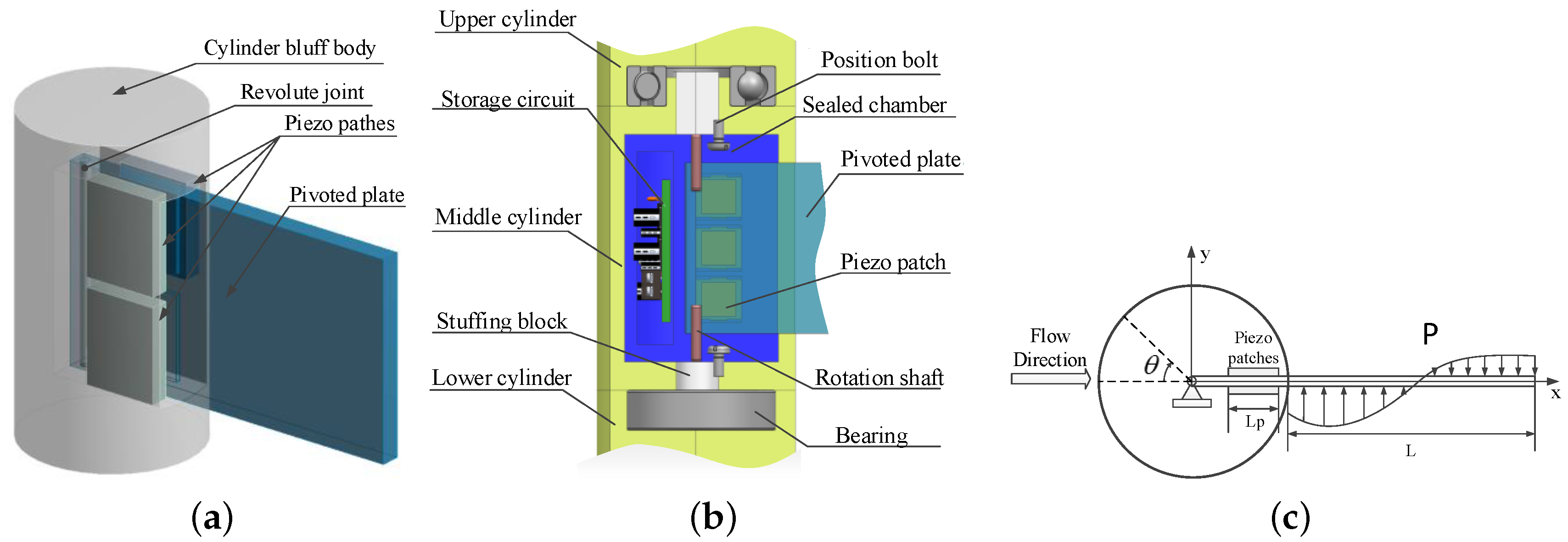
Underwater mooring platforms are tethered to the seabed using tens or hundreds of meters of mooring cables. Inspired by the above research, when a bluff body is covering the mooring cable, kinetic energy contained in vortices shed from the bluff body could be recovered through piezoelectric materials. A vortex-induced piezoelectric energy converter (VIPEC) for mooring cables is then designed as shown in Figure 1a. The VIPEC is intended to be affiliated to existing underwater mooring cables. It can be used to charge a storage battery and is beneficial for sustaining the cables’ stability. Furthermore, with the mooring cable as its foundation support, the VIPEC can be easily cascaded along the cable and scaled in size. The converter is mainly composed of a bluff body, a pivoted plate and several piezoelectric patches, and a storage circuit. When shedding vortices act on the pivoted plate, they squeeze piezo patches and convert fluid kinematic energy into electricity; generated electricity is collected through the storage circuit. Detailed mechanisms will be discussed in the following part.
The VIPEC is quite suitable for underwater mooring cables or other underwater mooring platforms (UMPs) due to its simple structure. However, its performance has never been researched before. This paper will investigate the characteristics of forces, the wake flow structure and the generated voltage of VIPECs of different design parameters with a computational fluid dynamic (CFD) method. The effects of the plate length under a certain range of Reynolds numbers are considered.
2. Description of the VIPEC
The VIPEC is mainly composed of a circular cylinder bluff body, a pivoted plate and several piezoelectric patches and a storage circuit. Two mechanisms, that is, the impingement of induced flow of shedding vortices on one side of the plate and the low-pressure region of vortices present at the opposite side of the plate, contribute the driving force, which drives the plate to squeeze its adjacent piezo patches to generate voltage. In order to eliminate the influence of the plate’s rotation on the cylinder, the cylinder is divided into three parts, and both the upper and lower parts are connected to the middle part by a bear, which ensures the middle part can rotate unrestrainedly under the action of wake flow on the plate, which ensures the plate will be in line with the flow direction to attain the minimal drag. The shaft’s friction is designed much smaller than that of the bearing, so that the narrow rotation of the plate does not cause the middle part to rotate. This converter is intended to be utilized in an underwater environment, such as covering cables of mooring platforms, and therefore underwater sealing is an inevitable problem. Electric components including piezo patches and the storage circuit are settled inside a sealed chamber. This can firstly guarantee those components isolated from water, and secondly they will have no influence on the plate’s rotation. Piezoelectric patches are amounted on either side of the plate inside the cylinder and a detailed view is shown in Figure 1b. A storage circuit is connected to piezo patches’ electrodes to collect charges and charge its accumulator persistently. It can discharge under a predetermined condition based on practical demands.
Physical Model
Since the plate remains in line with the flow direction, the cylinder’s rotation is not considered in this study. The rigid PVC (polyvinyl chloride) is taken to the attached plate, and its deformation can be ignored in comparison with its thickness and the rotation. Hence, it is considered to be undeformable. Since a straight pivoted plate is utilized in the wake, the converter has the same geometry in any cross-section along the plate’s height. Given the axial length does not affect the converter’s performance, a two-dimensional analysis was adopted in the present study. The plate is solely stuck with piezo patches in order to act stresses on patches adequately. Thus, the plate’s vibration amplitude is bounded and remains constant in all cases. It is the frequency and amplitude of stress that are essential factors to determine the VIPEC’s performance. Therefore, the plate is assumed to be stationary reasonably in the two-dimensional simulation. A principle diagram of a simplified physical model of the VIPEC due to vortex shedding is illustrated in Figure 1c. The cylinder’s center is selected as the coordinate origin. is the azimuth angle around the cylinder. P is the schematic distributed pressure on the plate, which is just an optional pressure distribution. Let D be the diameter of the cylinder and L be the plate length outside the cylinder. represents the patches’ length.
3. Mathematical Model
The two-dimensional CFD simulations presented in this paper were carried out on commercial code ANSYS Fluent 15.0, which is based on the cell-centered finite volume method.
3.1. Governing Equation and Turbulence Model
In this paper, the computational fluid dynamic simulation of the converter is conducted in unsteady incompressible viscous fluid. The governing equations are the Navier–Stokes equations including the continuity equation and the momentum equation, as written below:
where is the velocity component in the i direction, is the coordinate component in the i direction, is the fluid density, is its dynamic viscosity coefficient, p is the pressure.
Turbulence is modeled with the Reynolds averaging method, and the velocity is decomposed into the time-averaged and fluctuating components. The Reynolds stress model is adopted to close the unsteady Reynolds-averaged Navier–Stokes (URANS) equations, and the Reynolds stress tensor is written as:
where is the fluctuation velocity component in the i direction, is the turbulent viscosity, k is the turbulent energy and is the Kronecker delta.
The SST k- model is a hybrid model combing the k- and the k- models. It activates the k- model near the wall and the k- model in the free stream, which ensures it has better performance in the predictions of boundary layer flows with adverse pressure gradients. Therefore, the SST k- model is adopted in the CFD simulations of this paper.
3.2. Equations of Piezoelectric Performance
31-type piezoelectric patches were employed in the converter, which means the direction of polarization is perpendicular to that of applied stress. A resistance load () was connected to PZT (lead zirconate titanate piezoelectric ceramics) patches’ conductive electrodes for a simple analysis. In many cases, it is required to use a full wave rectifier for alternating current to direct current (AC–DC) conversion, which results in nonlinearity in the circuit dynamics. However, since the forcing term in the piezoelectric equation coming from the mechanical vibration and piezo patches is located on the cantilevered plate, the following analysis is considered with the reasonable assumption that the mechanical vibrations are not affected by the circuit dynamics [18].
Consider the following piezoelectric constitutive relation reduced from the tensorial representation [19]:
where is the electric displacement component, is the piezoelectric charge constant, is the stress component, is the permittivity electric constant, is the electric field component. can be expressed in terms of the voltage across the electrodes of pizeo patches, that is, (where is the thickness of the piezo layers). is derived from the lift force acting on the splitter plate and written as:
where is the ratio of the arm of lift force on the splitter to that of the normal stress acting on piezo patches, is the normal stress action area and is the lift force acting on the splitter plate. Thereafter, the circuit equation can be presented as:
The output voltage of the circuit equation can be extracted from Equation (6) and rearranged as:
The average output power can be calculated using the following relationship:
where is the period fo alternative lift force acting on the plate.
4. CFD Simulation Approach
4.1. Computational Domains and Grid Generation
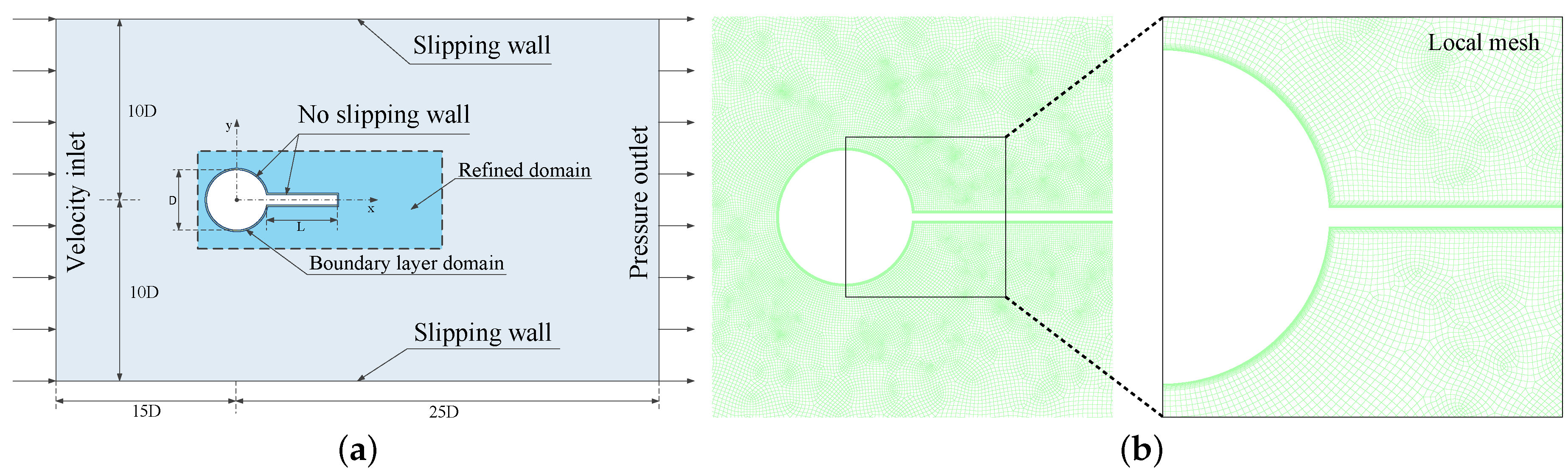
The computational domain had a width of and a length of (as showed in Figure 2a). The converter was placed in the symmetry of the top and bottom and at a distance of from the inlet boundary. Boundary conditions employed consisted of a velocity inlet on the left side, a pressure outlet on the right side and two slipping walls on the top and bottom sides.
The entire domain was discretized with quadrilateral elements. The domain around the converter was refined to obtain an accurate solution. Grids closest to the profiles of the converter were improved with rectangular elements to describe the boundary layer. The final grid around the converter and a local view is given in Figure 2b.
4.2. Solution Setups
A second-order upwind spatial discretization algorithm was used for all fluid-governing equations, including pressure, momentum and turbulence, and a least-squares cell-based algorithm was used for the gradient computation. The convection term and turbulence term were both discretized by the second-order upwind difference scheme in the present study. The second-order backward Euler scheme was employed to discretize the transient term. The second-order algorithm is more accurate than the first-order one because it reduces interpolation errors and false numerical diffusion. The coupled pressure–velocity coupling method was employed in all simulation cases. Convergences were determined by the magnitude of the governing equations’ residuals. The criteria of all scaled residuals including continuity equation, momentum equation, k equation and equation below were employed as the convergence criterion in order to get reliable results. The maximal iterations of each time step were set to 30, which enabled all residuals to reach convergence in every simulation case.
4.3. CFD Simulation Method Verification and Validation
Since no experimental results with the exact VIPEC model have been published yet, it is unrealistic to verify and validate the CFD method with experimental results. The VIPEC is working in a high Reynolds number flow in the practical application. Therefore, a verification and validation of whether the adopted CFD method could offer accurate results for high Reynolds number flow is conducted and compared with published results.
4.3.1. Verification
For the convenience of comparing with others’ simulated and experimental results, CFD simulation verification and validation in this paper was processed under flow past a smooth cylinder at . A grid convergence study was performed to evaluate the influence of grid resolution on the lift coefficient , the drag coefficient , and Strouhal number . Three different grid resolutions, whose total elements were controlled by max face size, and their calculated results are listed in Table 1. Because most elements were aggregated in the neighborhood of the model (the refined domain in Figure 2a), results of medium and fine grid cases had little difference. It can be noted that medium and fine girds gave substantially the same results and agree well with large eddy simulation (LES) results given by Catalano et al. [20], and published experimental data [21]. Considering time consumption in the simulation, the medium grid resolution was adopted in the following simulations.
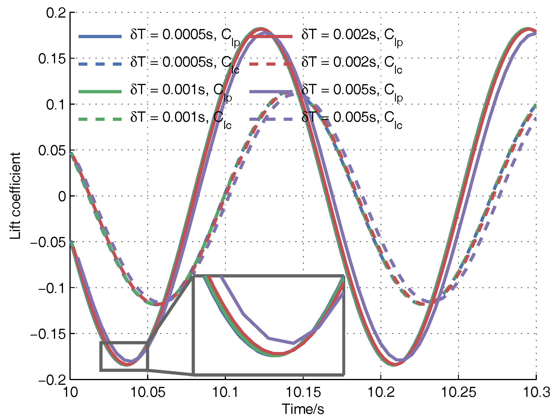
Based on the medium grid resolution, a time-step () verification was conducted with four different time steps for a cylinder with a plate of with reference to the root mean square (RMS) of lift coefficient and mean of drag coefficient on the plate and cylinder (termed as , , , , respectively). Their variation curves are shown in Figure 3 and corresponding results are summarized in Table 2. A small time step could not enhance the calculation accuracy too much and is time consuming. 0.002 s was set as the simulation time step in this paper, which is sufficient to gain precise solutions.
4.3.2. Validation
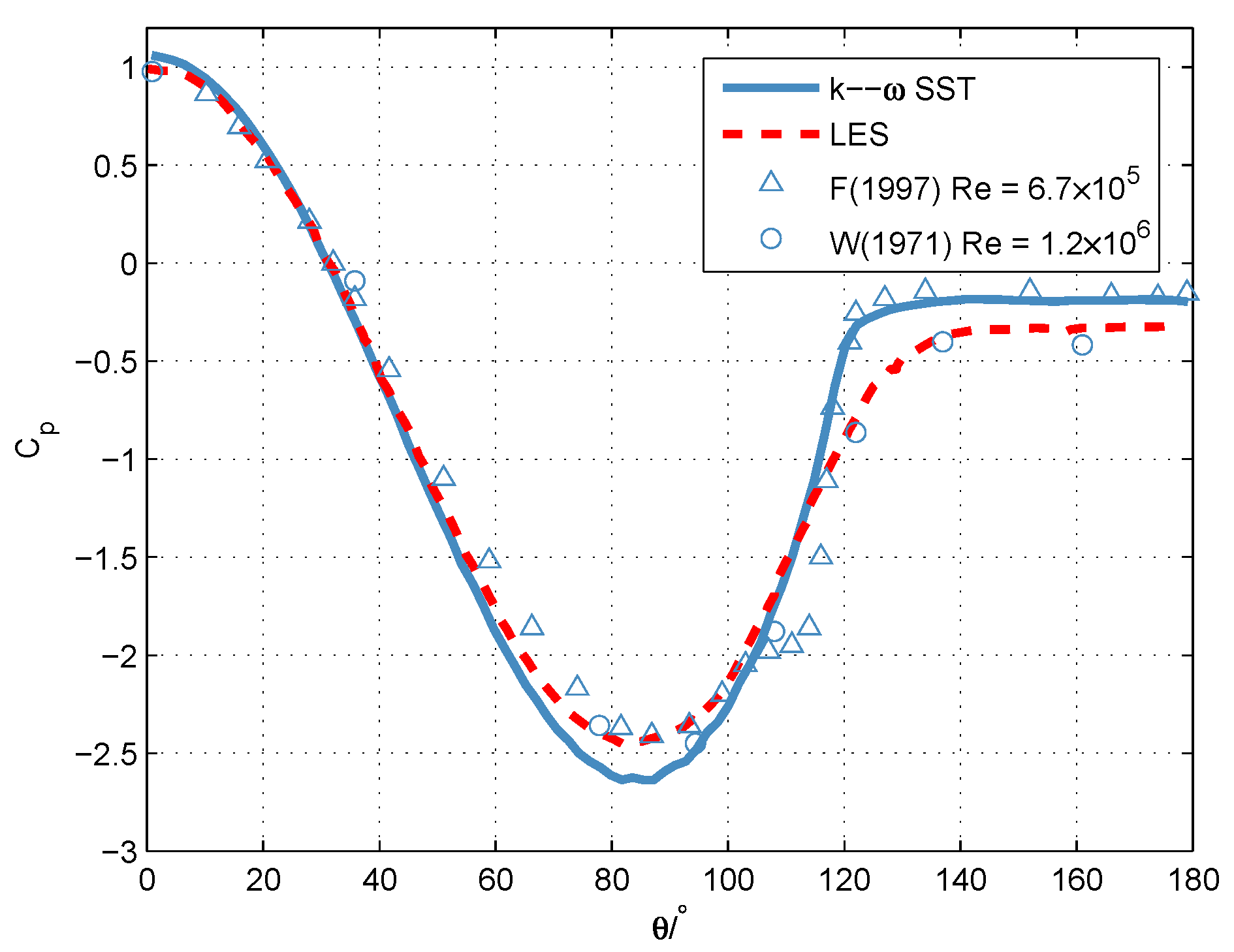
In order to validate the accuracy of the turbulent model adopted in this paper, the calculated pressure coefficient around the cylinder at is showed in Figure 4. It can be found that the simulation result agrees well with that of LES [20], Falchabart’s [21] and Warschauer and Leene’s [22] experiments, which means reliable results of this issue can be obtained from the adopted turbulent model.
5. Results and Discussion
5.1. Instantaneous Forces on the Splitter and Cylinder
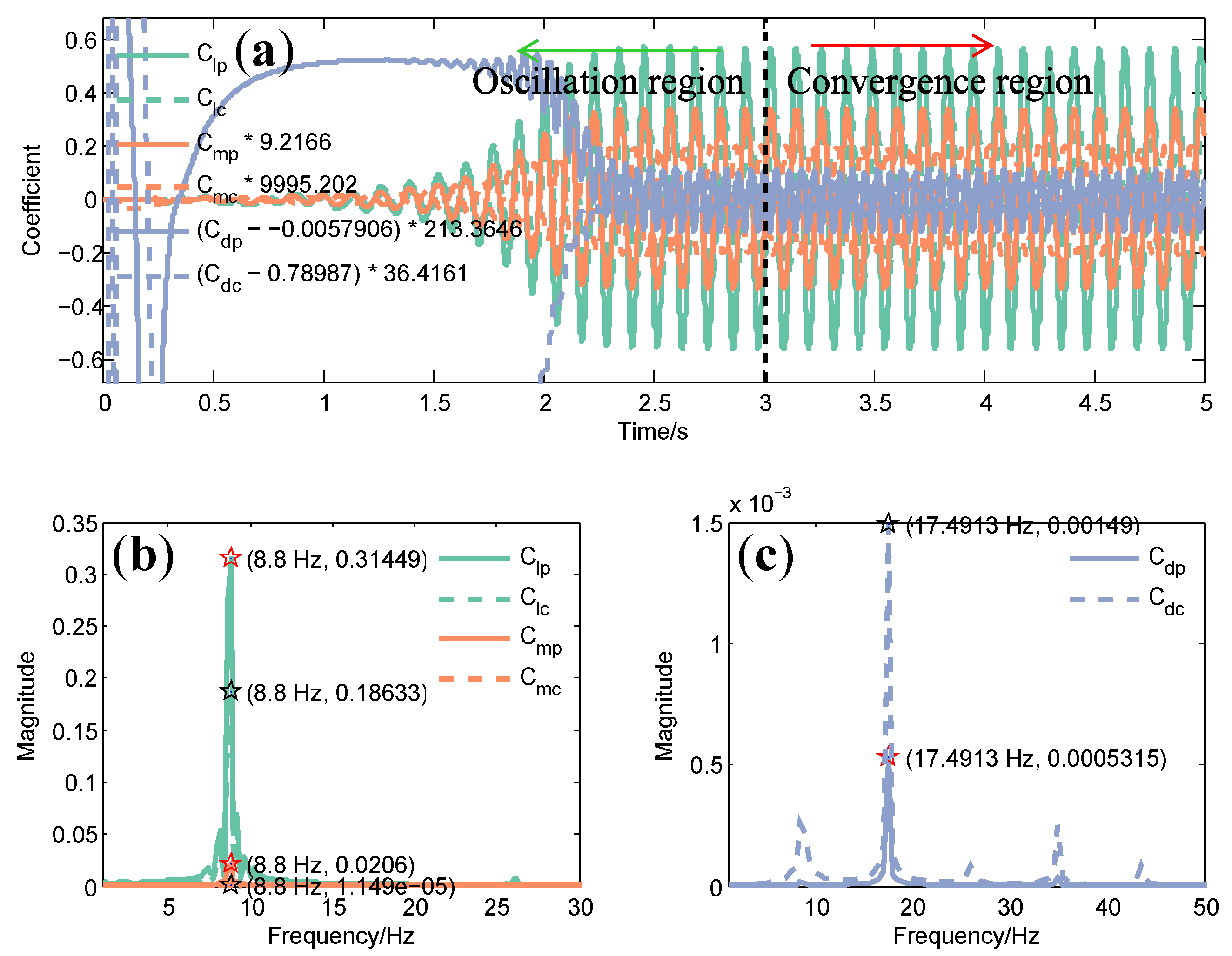
A series of simulation cases was carried out for various plate lengths, and the dimensionless plate length varied from 0.5 to 4 in an interval of 0.5 at a subcritical Reynolds number region of –. The selected Reynolds number range was based on the converter’s characteristic length and the flow velocity of its underwater working environment. Given the current flow velocity varies between m/s and 1.5 m/s in the underwater environment, D varies from 33 mm to 180 mm. The characteristic length D was fixed to 35 mm be the circular cylinder’s diameter, and the corresponding velocity changes from 1.4 m/s to 2.6 m/s according to the Reynold criterion in this paper. The case of U = 1.5 m/s and is selected for the illustration of instantaneous forces including the coefficients of lift and drag on the cylinder (termed as and , respectively), on the plate (termed as and , respectively) and the coefficient of torque (termed as and , respectively). To give a clear view at the same scale, the curves of and are offset by the mean value and all curves expect for and are magnified by an amplification factor, separately, as shown in Figure 5a. This reveals that all curves reach oscillatory convergence after 3 s. Therefore, every simulation in every case lasts for at least 30 s for all coefficients to reach their convergence, and only the last ten cycles are used to calculate the averaged coefficients.
The fast Fourier transforms (FFTs) for various instantaneous coefficients are conducted as shown in Figure 5b,c. It is observed that the dominant frequency for lift and momentum coefficients is 8.8 Hz. This indicates that each instantaneous coefficient’s fluctuation is controlled by shedding vortices and hence they share the same frequency. However, since each vortex has the same contribution to the drag, ’s and ’s frequency is twice (17.49 Hz) that of lift coefficient.
5.2. Analysis of Wake Structure
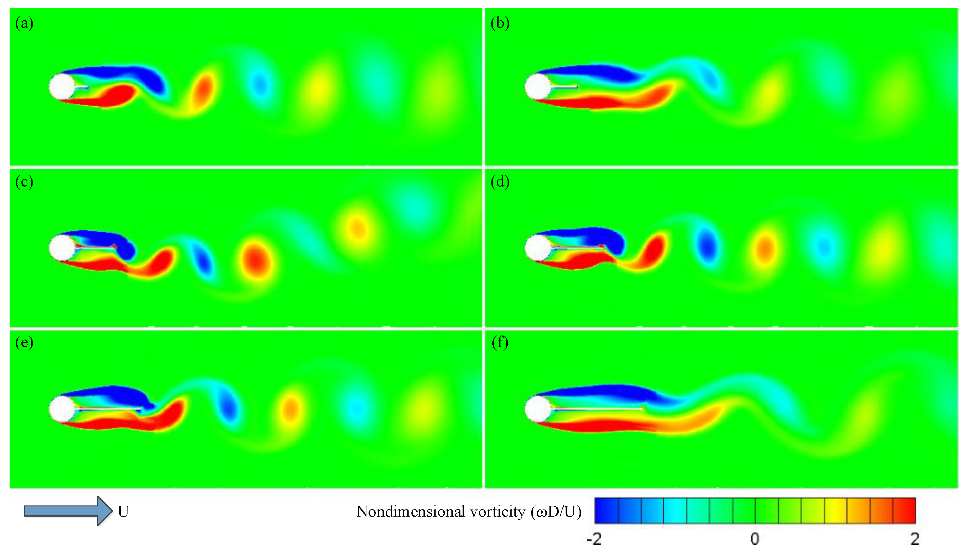
In order to investigate the influence of the plate length on the wake structure of the converter, contours of nondimensional vorticity for a variety of plate lengths at U = 1.7 m/s are illustrated in Figure 6. The wake shows a regular 2S vortex pattern (a single vortex is shed into the downstream in each half cycle) for varied splitter lengths, which means the plate has little impact on the far downstream wake. Shedding vortices cannot roll from one side to the other side along the cylinder’s rear surface due to the plate’s prevention, thus they are forced to process along the plate downstream. Therefore, with the existence of the plate, the shear layer is greatly influenced and extended to the tip of the plate, and the near-plate wake field is significantly rebuilt, which results in dissimilar shapes of lift force curves. Shedding vortices cannot attach to the plate for , and they reattach to the plate for longer s. Meanwhile, the vorticity magnitude is obviously smaller at compared with other cases, and vorticity contour becomes approximately symmetrical over the plate. Additionally, the reattachment of shedding vortices (Figure 6c–e) on the splitter leads to a counterflow along its surfaces, which also contributes to a larger negative-pressure region and higher pressure difference between two surfaces.
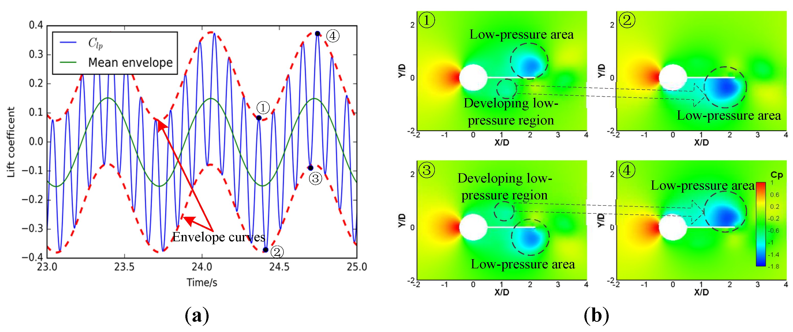
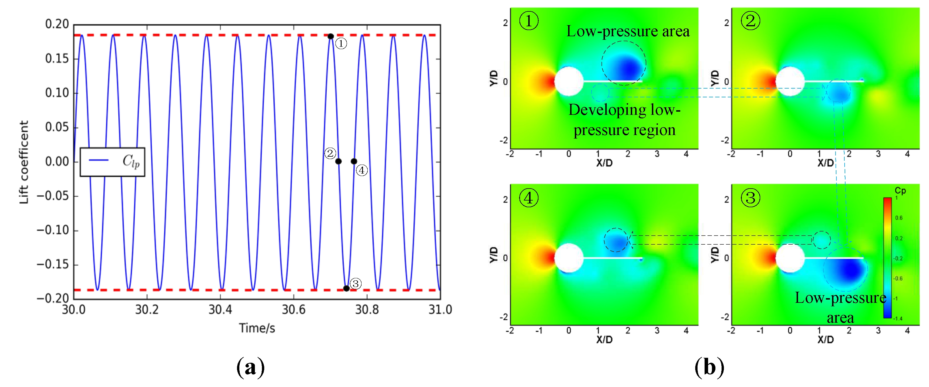
In order to show the variation of the wake structure at different design parameters, time-varying lift-coefficient and pressure-coefficient contours are presented in Figure 7 in comparison with that of another simulation case as shown in Figure 8. In order to compare variations of the wake structure, time-varying lift-coefficient and pressure- coefficient contours of two simulation cases with significant differences are presented in Figure 7 and Figure 8. It can be found that the variation of lift coefficient is obviously different from other simulation cases in Figure 7. Two dominant frequencies (Figure 7a) shape the varying lift force, while the upper/lower envelope and mean value oscillate synchronously with the same frequency, which is the major oscillating frequency of the lift coefficient. The minor frequency is produced as a result of the developing low-pressure area marching alongside one surface of the plate. Lift-force peaks are obtained when the low-pressure area reaches the tip of the plate (Figure 7b). Furthermore, the maximum of negative pressure is obviously greater for the case shown in Figure 7 than that shown in Figure 8, which determines its lift coefficient has a larger amplitude.
5.3. Analysis of the Driving Force
The lift force acting on the plate performs as the driving force on piezo patches. Its dimensionless shedding frequency, phase difference of lifts on the upper/lower surface, RMS of and its arm are all analyzed in the following part.
5.3.1. Dimensionless Shedding Frequency
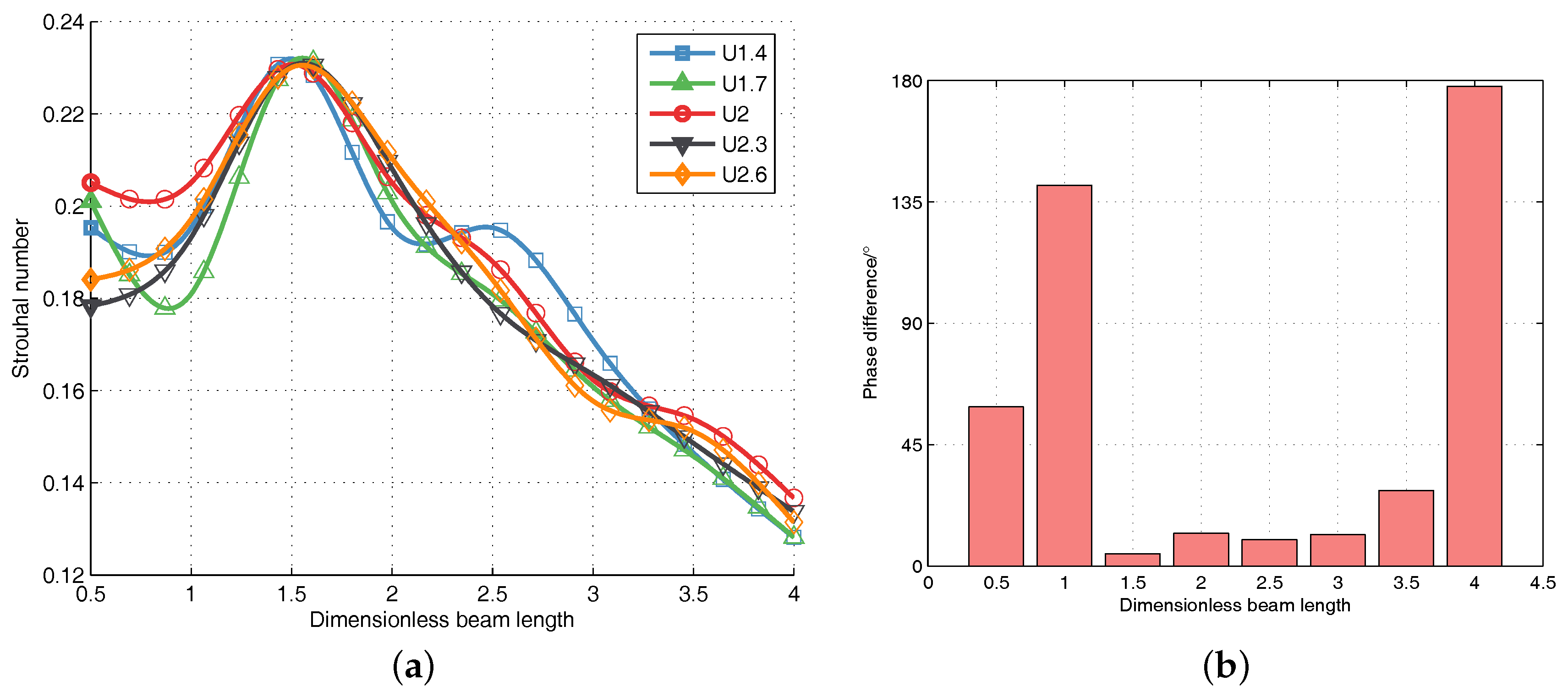
Influence of plate length on dimensionless shedding frequency (Strouhal number) is shown in Figure 9a. It reveals that the variation of Strouhal number obeys the same tendency for the selected Reynolds number range. It grows with the increment of the plate’s length for , though the tendency seems to be slightly diminished at around . All s reach a maximum of at , and this is also the condition when maximal RMS of comes up. This indicates that the shedding vortices are distinctly affected by their reattachment on the plate. decreases almost linearly with the growth of the plate’s length for .
5.3.2. Phase Difference
The lift force exerting on the plate is the summation of those acting on its lower side and upper surface. The existence of the splitter not only affects the lifts’ amplitude but also their phase. Pressure centers on each surface are obviously not equivalent and the maximum of negative pressure does not remain constant, as shown in the pressure contour (Figure 7 and Figure 8). This nonequivalence results in a fluctuating phase difference between the forces on lower and upper surfaces. Phase differences of lifts at different plate lengths are averaged and illustrated in Figure 9b. It can be noted that the phase difference of is remarkably greater than other cases, which could result in a lift coefficient of a small amplitude. The fluctuating phase difference and absolute pressure difference together shape the time-varying total lift on the plate.
5.3.3. RMS of
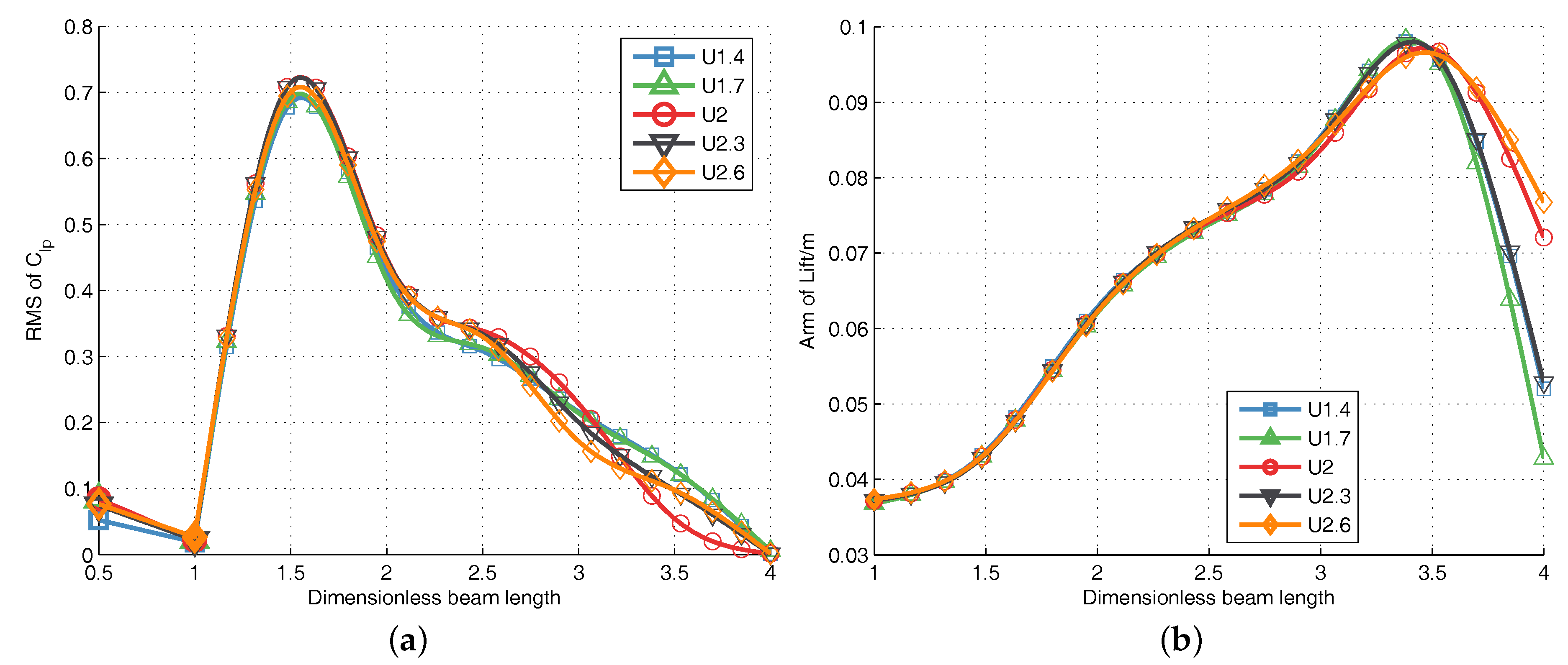
The amplitude of lift coefficient is characterized by its RMS value, and the variation of RMS of is presented in Figure 10a. It can be noticed that a sinking of exists at , which is caused by the wake being approximately symmetric at the plate’s upper/lower surface (Figure 6b) due to shedding vortices not adhering to its surfaces. RMS of reaches it peak at for different velocities, and it begins to decline due to the combined effect of the magnitude of negative pressure region on the plate (Figure 7 and Figure 8) and the phase difference between the lift on both sides (Figure 9b).
5.3.4. Arm of Lift
The arm-of-lift force on the plate is calculated by . As shown in Figure 10b, the lift arm almost increases linearly as the plate’s length grows for . It results from shedding vortices’ propagation along the plate’s span direction. The lift arm has a certain degree of decline at . This is due to the wake zone being approximately symmetrical and steady, which results in a smaller fluctuating lift and a shorter lift arm.
This demonstrates that the dimensionless shedding frequency , the phase difference between the on the plate’s upper/lower surface, the RMS and the arm () with reference to the lift force on the plate () all behave with the same tendency and approximately in the same magnitude. This indicates that at the simulated subcritical Reynolds number region, the influence of Reynolds number on the driving force is not enough to be noticeable.
5.4. Analysis of the System Performance
5.4.1. Output Voltage
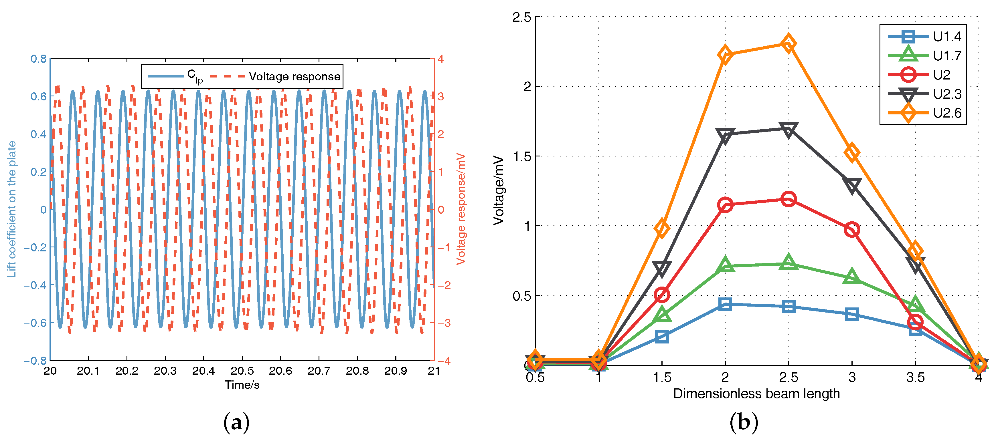
With a resistance load of 10 M, the voltage response of piezo patches along with the calculated lift force on the splitter for the simulation case U = 2.6 m/s and is shown in Figure 11a. Table 3 lists the major properties of the adopted piezoelectric material for piezo patches. It should be noted that in Figure 11a, phase difference exists obviously between the and responding voltage responses due to the partial derivative term with respect to time in Equation (7). Nevertheless, their fluctuation frequencies remain the same, which equals the vortex shedding frequency.
RMS of voltage (term as ) in different simulation cases varying versus the dimensionless plate length is given in Figure 11b. Because of the tiny lift on the plate, s get close to 0 at for various inlet velocities. s reach their maxima at . The maximum of RMS of output voltage is around 2.3 mV with U = 2.6 m/s and . The generated output could be collected through a storage circuit, or charge an accumulator, and it can discharge periodically or at predetermined conditions, which proves the feasibility of the VIPEC.
5.4.2. Output Power and Power Density
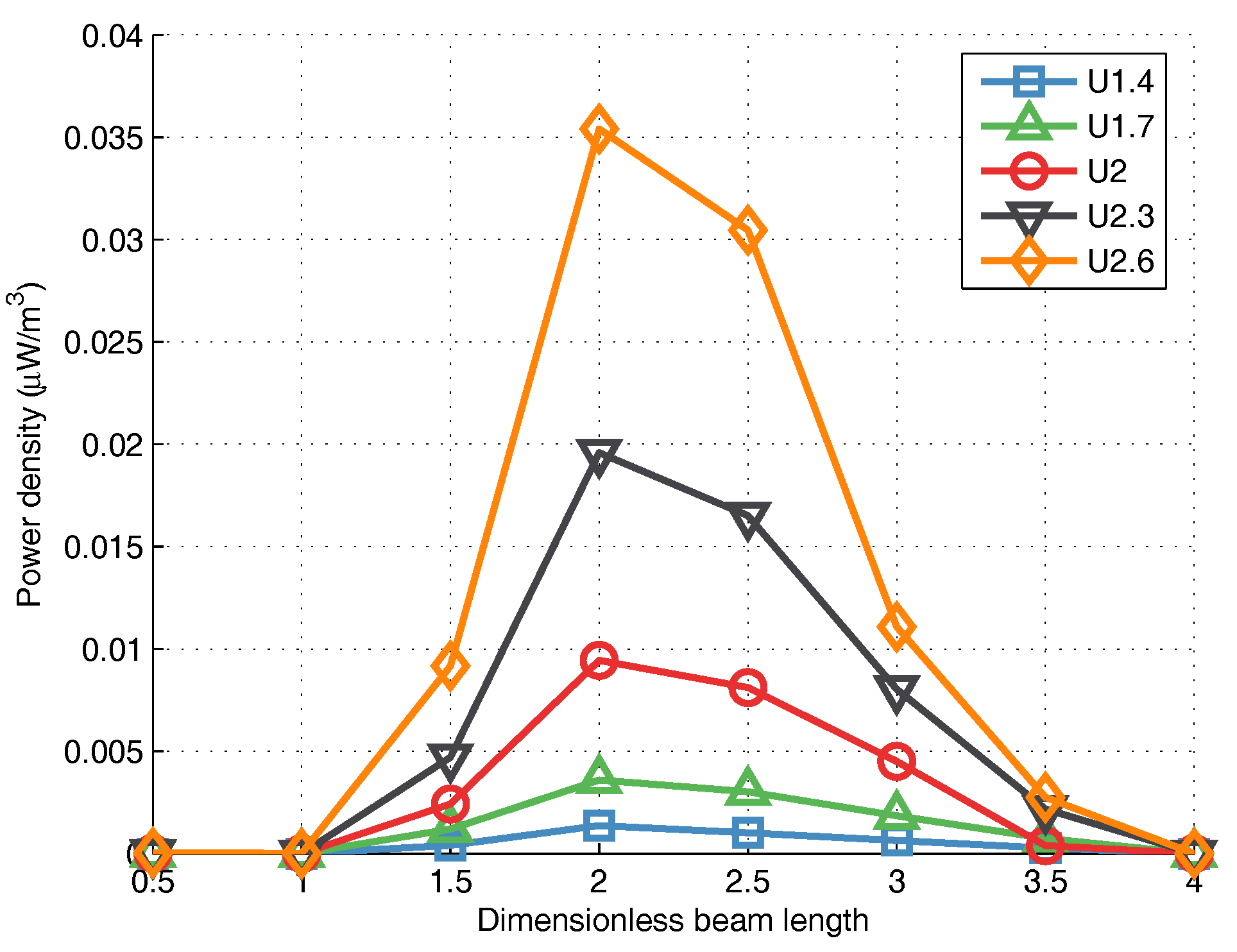
With the calculated output power from Equation (8), power density per sweep volume [10], defined as power value divided by stalk’s volume (microwatt per cubic meter), is calculated and presented in Figure 12. The maximal power density reaches 0.035 W/m at and U = 2.6 m/s. Though it is quite small compared with those of Pobering and Schwesinger [5] (theoretically 68.1 W/cm), Li et al. [6] (2036 W/cm), Akaydin et al. [10] (23.6 mW/m) and Vatansever et al. [7] (157.9 W/cm for the PVDF layer, 9.67 W/cm for the PZT–single layer and 2.28 W/cm for the PZT–bimorph in the air), the VIPEC could be easily cascaded in a single mooring cable. Besides, the smaller lift coefficient on the cylinder makes the cable more stable. Periodical discharge from the storage circuit provides multiple purposes of the VIPEC.
6. Conclusions
A novel form of a vortex-induced piezoelectric energy converter (VIPEC) was introduced in this paper. Its voltage response equation was established based on the constitutive relations of piezoelectric materials. Utilizing a simplified physical model, two-dimensional transient CFD simulations with a k- turbulence model were conducted to investigate the variation of the wake structure and the driving force under various conditions of inlet velocities and plate lengths. Finally, the effect of the plate length on the performance of the converter was studied and the results demonstrate the design of the VIPEC is feasible.
Important conclusions of this study are summarized below:
- With the growth of the plate length, , , and increase at first and decrease subsequently due to the reattachment of shedding vortices on the plate, though they reach their peaks at different plate lengths. The optimal plate length for the maximal and is and , respectively, for maximal .
- Under the simulated Reynolds number region, the different aspects of the driving force (, phase difference, RMS of , ) have the same variation shapes, and the influence of the Reynolds number on the driving force is not very explicit.
- The wake structure under different situations at the subcritical Reynolds number region is similar to the Kármán vortex street in the 2S pattern. The plate has two principal effects on the flow structure and hydrodynamic forces of the converter. Firstly, it prevents shedding vortices rolling from one side to the other side along the rear of the cylinder. Secondly, it extends the length of the shear layer and delays the obvious shedding of vortices.
- The peaks of voltage response are obtained at with the inlet velocity as 2.6 m/s and the maximum of RMS of output voltage around 2.3 mV. The maximal averaged power density reaches 0.035 W/m at and U = 2.6 m/s with a resistance load of 10 M.
Acknowledgments
This research was supported by the National Natural Science Foundation of China (Grant No. 51179159, 61572404).
Author Contributions
Xinyu An conceived the study and performed the CFD simulations; Xinyu An, Baowei Song and Wenlong Tian analyzed the simulation results; Xinyu An wrote the manuscript; Wenlong Tian and Congcong Ma reviewed and edited the manuscript.
Conflicts of Interest
The authors declare no conflict of interest.
References
- Rostami, A.B.; Armandei, M. Renewable energy harvesting by vortex-induced motions: Review and benchmarking of technologies. Renew. Sustain. Energy Rev. 2017, 70, 193–214. [Google Scholar] [CrossRef]
- Bernitsas, M.M.; Raghavan, K.; Ben-Simon, Y.; Garcia, E.M.H. VIVACE (vortex-induced Vibration for Aquatic Clean Energy): A New Concept in Generation of Clean and Renewable Energy from Fluid Flow. J. Offshore Mech. Arct. Eng. Trans. ASME 2008, 130, 619–636. [Google Scholar] [CrossRef]
- Bernitsas, M.M.; Ben-Simon, Y.; Raghavan, K.; Garcia, E.M.H. The VIVACE Converter: Model Tests at High Damping and Reynolds Number Around 105. J. Offshore Mech. Arctic Eng. 2009, 131, 403–414. [Google Scholar] [CrossRef]
- Taylor, G.W.; Burns, J.R.; Kammann, S.M.; Powers, W.B.; Welsh, T.R. The Energy Harvesting Eel: A Small Subsurface Ocean/River Power Generator. IEEE J. Ocean. Eng. 2001, 26, 539–547. [Google Scholar] [CrossRef]
- Pobering, S.; Schwesinger, N. A novel hydropower harvesting device. In Proceedings of the IEEE International Conference on MEMS, NANO and Smart Systems, Banff, AB, Canada, 25–27 August 2004; pp. 480–485. [Google Scholar]
- Li, S.; Yuan, J.; Lipson, H. Ambient wind energy harvesting using cross-flow fluttering. J. Appl. Phys. 2011, 109, 109–111. [Google Scholar] [CrossRef]
- Vatansever, D.; Hadimani, R.L.; Shah, T.; Siores, E. An investigation of energy harvesting from renewable sources with PVDF and PZT. Smart Mater. Struct. 2011, 20, 55019–55024. [Google Scholar] [CrossRef]
- Oh, S.J.; Han, H.J.; Han, S.B.; Lee, J.Y.; Chun, W.G. Development of a tree-shaped wind power system using piezoelectric materials. Int. J. Energy Res. 2010, 34, 431–437. [Google Scholar] [CrossRef]
- Akaydin, H.D.; Elvin, N.; Andreopoulos, Y. Wake of a cylinder: A paradigm for energy harvesting with piezoelectric materials. Exp. Fluids 2010, 49, 291–304. [Google Scholar] [CrossRef]
- Akaydin, H.D.; Elvin, N.; Andreopoulos, Y. The performance of a self-excited fluidic energy harvester. Smart Mater. Struct. 2012, 21, 25007–25019. [Google Scholar] [CrossRef]
- Dai, H.L.; Abdelkefi, A.; Wang, L. Piezoelectric energy harvesting from concurrent vortex-induced vibrations and base excitations. Nonlinear Dyn. 2014, 77, 967–981. [Google Scholar] [CrossRef]
- An, X.; Song, B.; Mao, Z.; Ma, C. The mathematical modeling of a novel anchor based on vortex-induced vibration. In Proceedings of the IEEE Oceans, Shanghai, China, 10–13 April 2016; pp. 1–5. [Google Scholar]
- Kwon, K.; Choi, H. Control of laminar vortex shedding behind a circular cylinder using splitter plates. J. Mech. Sci. Technol. 2014, 28, 1721–1725. [Google Scholar] [CrossRef]
- Vu, H.C.; Ahn, J.; Hwang, J.H. Numerical investigation of flow around circular cylinder with splitter plate. KSCE J. Civil Eng. 2016, 20, 2559–2568. [Google Scholar] [CrossRef]
- Gerrard, J.H. The mechanics of the formation region of vortices behind bluff bodies. J. Fluid Mech. 1966, 25, 401–413. [Google Scholar] [CrossRef]
- Apelt, C.J.; West, G.S.; Szewczyk, A.A. The effects of wake splitter plates on the flow past a circular cylinder in the range 104 < R < 5 × 10⁴. J. Fluid Mech. 1973, 61, 187–198. [Google Scholar]
- Apelt, C.; West, G. The effects of wake splitter plates on bluff-body flow in the range 104 < R < 5 × 10⁴. Part 2. J. Fluid Mech. 1975, 71, 145–160. [Google Scholar]
- Erturk, A.; Tarazaga, P.A.; Farmer, J.R.; Inman, D.J. Effect of Strain Nodes and Electrode Configuration on Piezoelectric Energy Harvesting From Cantilevered Beams. J. Vib. Acoust. 2009, 131, 402–413. [Google Scholar] [CrossRef]
- Meitzler, A.; Tiersten, H.F.; Warner, A.W.; Berlincourt, D.; Couqin, G.A.; Welsh, F.S., III. IEEE Standard on Piezoelectricity; American National Standards Institute: New York, NY, USA, 1988. [Google Scholar]
- Catalano, P.; Wang, M.; Iaccarino, G.; Moin, P. Numerical simulation of the flow around a circular cylinder at high Reynolds numbers. Int. J. Heat Fluid Flow 2003, 24, 463–469. [Google Scholar] [CrossRef]
- Zdravkovich, M.M. Conceptual overview of laminar and turbulent flows past smooth and rough circular cylinders. J. Wind Eng. Ind. Aerodyn. 1990, 33, 53–62. [Google Scholar] [CrossRef]
- Warschauer, K.A.; Leene, J.A. Experiments on mean and fluctuating pressures of circular cylinders at cross flow at very high Reynolds numbers. In Proceedings of the International Conference on Wind Effects on Buildings and Structures, Tokyo, Japan, 16–18 September 1971; pp. 305–315. [Google Scholar]
Figure 1.
Components of the vortex-induced piezoelectric energy converter (VIPEC): (a) a general view, (b) an inside view and (c) a principle diagram of the simplified two-dimensional model.
Figure 1.
Components of the vortex-induced piezoelectric energy converter (VIPEC): (a) a general view, (b) an inside view and (c) a principle diagram of the simplified two-dimensional model.

Figure 2.
(a) Computation domains and boundary conditions; (b) computing mesh and a local detail view.
Figure 2.
(a) Computation domains and boundary conditions; (b) computing mesh and a local detail view.

Figure 3.
Verification of the lift coefficient with different time steps ( is the time step; and is the lift coefficient on the plate and the cylinder, respectively).
Figure 3.
Verification of the lift coefficient with different time steps ( is the time step; and is the lift coefficient on the plate and the cylinder, respectively).

Figure 4.
Pressure distribution around the cylinder compared with others’ simulation and experimental results.
Figure 4.
Pressure distribution around the cylinder compared with others’ simulation and experimental results.

Figure 5.
(a) The time history of coefficients of instantaneous forces, (b) the frequency spectra of , , , and (c) , for the simulation of U = 1.5 m/s and .
Figure 5.
(a) The time history of coefficients of instantaneous forces, (b) the frequency spectra of , , , and (c) , for the simulation of U = 1.5 m/s and .

Figure 6.
Wake structures in the form of nondimensional vorticity at U = 1.7 m/s for various plate lengths: (a) ; (b) ; (c) ; (d) ; (e) and (f) .
Figure 6.
Wake structures in the form of nondimensional vorticity at U = 1.7 m/s for various plate lengths: (a) ; (b) ; (c) ; (d) ; (e) and (f) .

Figure 7.
(a) Instantaneous lift ( is the lift coefficient on the plate) and (b) pressure-coefficient contours around the plate with U = 1.7 m/s and .
Figure 7.
(a) Instantaneous lift ( is the lift coefficient on the plate) and (b) pressure-coefficient contours around the plate with U = 1.7 m/s and .

Figure 8.
(a) Instantaneous lift ( is the lift coefficient on the plate) and (b) pressure-coefficient contours around the splitter with U = 2 m/s and .
Figure 8.
(a) Instantaneous lift ( is the lift coefficient on the plate) and (b) pressure-coefficient contours around the splitter with U = 2 m/s and .

Figure 9.
Variation of (a) Strouhal number ; (b) phase difference between lift coefficients on the upper and lower surfaces of the plate versus the dimensionless plate length at different velocities.
Figure 9.
Variation of (a) Strouhal number ; (b) phase difference between lift coefficients on the upper and lower surfaces of the plate versus the dimensionless plate length at different velocities.

Figure 10.
Variation of (a) RMS of and (b) the arm of versus the dimensionless plate length.

Figure 11.
(a) and corresponding voltage response versus time for U = 2.6 m/s and ; (b) RMS of voltage response for different plate lengths under various velocities. All loads were 10 M.
Figure 11.
(a) and corresponding voltage response versus time for U = 2.6 m/s and ; (b) RMS of voltage response for different plate lengths under various velocities. All loads were 10 M.

Figure 12.
The averaged density of output power for different plate lengths under various velocities.
Figure 12.
The averaged density of output power for different plate lengths under various velocities.


Table 1.
Simulation validation ( and is the lift and drag coefficient on the cylinder, is the corresponding Strouhal number).
Table 1.
Simulation validation ( and is the lift and drag coefficient on the cylinder, is the corresponding Strouhal number).
| Max Face Size | Total Elements | ||||
|---|---|---|---|---|---|
| Coarse | 60 | 68,000 | 0.081 | 0.40 | 0.268 |
| Medium | 30 | 70,000 | 0.090 | 0.35 | 0.323 |
| Fine | 15 | 89,000 | 0.092 | 0.33 | 0.327 |
| LES (Large Eddy Simulation) [20] | - | - | - | 0.31 | 0.35 |
| Published experimental data [21] | - | - | 0.21–0.63 | 0.17–0.40 | 0.18–0.50 |
Table 2.
RMS of lift and mean of drag coefficient at different time steps.
| Time Step ()/s | RMS of | RMS of | Mean of | Mean of |
|---|---|---|---|---|
| 0.0005 | 0.130046 | 0.081676 | 0.004463 | 0.721799 |
| 0.001 | 0.130107 | 0.081739 | 0.004463 | 0.721808 |
| 0.002 | 0.129713 | 0.081442 | 0.004462 | 0.721767 |
| 0.005 | 0.126406 | 0.079282 | 0.004455 | 0.721411 |
Table 3.
Major properties for adopted piezoelectric patches.
| Physical Property | Value |
|---|---|
| Vacuum permittivity (pF/m) | 8.85 |
| Permittivity electric constant | 1700 |
| Piezoelectric charge constant (pm/V) | −171 |
| Thickness (mm) | 2 |
| Electrode area (mm) | 20 |
| Stress area (mm) | 255 |
© 2018 by the authors. Licensee MDPI, Basel, Switzerland. This article is an open access article distributed under the terms and conditions of the Creative Commons Attribution (CC BY) license (http://creativecommons.org/licenses/by/4.0/).
Share and Cite
MDPI and ACS Style
An, X.; Song, B.; Tian, W.; Ma, C. Design and CFD Simulations of a Vortex-Induced Piezoelectric Energy Converter (VIPEC) for Underwater Environment. Energies 2018, 11, 330. https://doi.org/10.3390/en11020330
AMA Style
An X, Song B, Tian W, Ma C. Design and CFD Simulations of a Vortex-Induced Piezoelectric Energy Converter (VIPEC) for Underwater Environment. Energies. 2018; 11(2):330. https://doi.org/10.3390/en11020330
Chicago/Turabian StyleAn, Xinyu, Baowei Song, Wenlong Tian, and Congcong Ma. 2018. "Design and CFD Simulations of a Vortex-Induced Piezoelectric Energy Converter (VIPEC) for Underwater Environment" Energies 11, no. 2: 330. https://doi.org/10.3390/en11020330
Note that from the first issue of 2016, this journal uses article numbers instead of page numbers. See further details here.