Predicting Human Location Using Correlated Movements


1
Department of Electrical and Computer Engineering, University of Ulsan, Ulsan 44610, Korea
2
School of Computer Science and Engineering, Nanyang Technological University, Singapore 639798, Singapore
*
Author to whom correspondence should be addressed.
Electronics 2019, 8(1), 54; https://doi.org/10.3390/electronics8010054
Submission received: 24 October 2018
/
Revised: 8 December 2018
/
Accepted: 2 January 2019
/
Published: 3 January 2019
(This article belongs to the Section Computer Science & Engineering)
Abstract
:This paper aims at estimating the current location, or predicting the next location, of a person when the recent location sequence of that person is unknown. Inspired by the fact that the behavior of an individual is greatly related to other people, a two-phase framework is proposed, which first finds persons who have highly correlated movements with a person-of-interest, then estimates the person’s location based on the position information for selected persons. For the first phase, we propose two methods: community interaction similarity-based (CISB) and behavioral similarity-based (BSB). The CISB method finds persons who have similar encounters with other members in the entire community. In the BSB method, members are selected if they show similar behavioral patterns with a given person, even though there are no direct encounters or evident co-locations between them. For the second phase, a neural network is considered in order to develop the prediction model based on the selected members. Evaluation results show that the proposed prediction model under the BSB scheme outperforms other methods, achieving top-1 accuracy of 71.13% and 69.36% for estimations of current and next locations, respectively, with the MIT dataset and 92.31% and 92.03% in case of the Dartmouth dataset.
1. Introduction
Human mobility prediction can be used in many potential and promising applications, such as location-based recommendation services, contagious disease control, patient tracking, geographic profiling, and urban planning [1,2,3,4,5]. In particular, in order to prevent the outbreak of infectious diseases (e.g., malaria and flu), which usually spread due to people’s travels and interactions, estimating the location of persons who are at a high risk of infection is crucial [1,4]. In geographic profiling, in order to strengthen security, law enforcement agencies need to analyze movements of suspects and need to determine their most likely position [5].
If someone’s recent location is known using a global positioning system (GPS) or other localization techniques (e.g., Wi-Fi, cellular-based systems), it is relatively simple to estimate that person’s current or next locations. However, there are cases where someone’s recent location sequences are not available. For instance, the GPS function is required to turn off due to lack of battery power in a smartphone even though people want to share their positions. In addition, there are some cases where data is sparse [6,7] (e.g., call detail records, health record of individuals, and credit card spending data). Moreover, in some cases, it is necessary to estimate locations even when someone may not want to share that information (e.g., geographic profiling of criminals). Therefore, in this work, we consider a new problem which is estimating someone’s current or next location, particularly when recent location sequence information is not available.
Specifically, the mobility information of other Persons with Correlated Movements (PCM) with a given person is used to estimate the person-of-interest’s current or future location, based on the fact that the behavior of one individual is largely related to other members. In other words, the current or next location of a given person is estimated using the known position information of other specific people. Although there were several studies on the prediction of human location using social relationships [8,9,10], those works focused on finding direct social ties between people (e.g., friendships) using encounters or calling traces between them. However our work, in addition to friendships, considers behavioral similarity between people, which may not be reflected by direct encounters or co-location events between them.
In this paper, we propose a two-phase human location prediction model. More specifically, in the first phase, PCMs with a given person are selected. For this phase, two novel PCM selection methods are proposed: community interaction similarity-based (CISB) and behavioral similarity-based (BSB). In the CISB method, interactions with other community members are considered as well as direct encounters between certain individuals, i.e., the strength of the social relationship between people is measured by not only their direct interactions but also their interactions with other members of society. The motivation is that if two people have a close social tie, then they may have similar patterns of meeting other members of the community. In contrast to the CISB method, which attempts to find PCMs with stronger social ties, the objective of the BSB method is to find PCMs with similar behavioral patterns. As a result, the selected PCMs under the BSB method may not have a strong social relationship with the person-of-interest. In the second phase, motivated by the fact that the movement of an individual is highly correlated with other people, the current or next location of a person is estimated using the position information of selected PCMs. A PCM-based location prediction (PLP) model is developed based on a neural network (NN) [11].
For this paper, two different datasets were used to evaluate the proposed prediction model. The first dataset provided cellular traces collected by the Massachusetts Institute of Technology (MIT) Media Lab [12], which recorded the time a mobile phone was associated with a base station. In a metropolitan area, small and short-range cells that cover distances of a few hundred meters are more popular [13]. Moreover, since people usually carry their phones all the time, the position of a base station can be used to represent a person’s approximate location [10,14,15,16,17,18]. The second dataset is the mobility data extracted from Wi-Fi traces collected in the Dartmouth university campus [19]. A log message was recorded whenever a mobile device associates or disassociates with an AP. Due to the relatively short range of the Wi-Fi technology, an AP can be used to reflect a person’s location [20,21,22].
Experiments were performed in order to validate the proposed prediction model in various situations. We draw a comparison between the designed PLP model and the baseline one, called most frequent location (MFL), in which the most visited position is predicted as the location of the person-of-interest. Two proposed PCMs selection methods are also compared with three recent existing approaches: encounter frequency-based (EFB) [18,23,24], spatial closeness (SC) [6], and spatio-temporal closeness (STC) [6]. Specifically, EFB is rooted in encounter frequency, which is one of the natural characteristics of a friendship, i.e., two members who more frequently meet each other are likely to be closer friends. In SC, the persons who have the most similar distribution of visited locations to the person-of-interest are selected, meanwhile STC chooses members with the most synchronous movement with that of the person-of-interest.
The main contributions of our work can be summarized as:
- Our work considers a new problem in which human location should be estimated in a challenging situation, i.e., the recent historical location of the person-of-interest is not available. To address this challenge, a two-phase framework with low time and space complexity is proposed. Specifically, for a given person-of-interest, persons with correlated movements (PCMs) are first selected, then the location of the person-of-interest is estimated based on the spatio-temporal information of selected PCMs.
- Two novel PCMs selection methods are proposed: CISB and BSB. CISB selects PCMs who have the strongest social tie with the person-of-interest. Because socially close people may have similar patterns of meeting other members in the community, CISB finds persons who have similar encounters with other members.
- While the purpose of CISB is to find PCMs who have the strong social relationship with the person-of-interest, BSB aims at selecting PCMs who have similar behavior patterns with the person-of-interest, even though there may be no direct encounters or evident co-location between them. As a result, the selected PCMs under the BSB method may not have strong social tie with the person-of-interest.
- A PCM-based location prediction model, which leverages the recent spatial data of selected PCMs, is developed.
- Experimental results show that the performance of BSB substantially dominates other PCMs selection methods in terms of prediction accuracy. In addition, higher performance can be achieved when a larger number of PCMs are embedded into the model. In particular, a beneficial effect of a large number of PCMs is more clearly observed in case of BSB than other PCMs extraction methods.
The rest of this manuscript is organized as follows. Section 2 and Section 3 discuss related studies of human mobility prediction and the two considered datasets, respectively. Then, the proposed framework is described briefly in Section 4. In Section 5, two methods for selecting PCMs in the first phase are presented. Section 6 explains the PCM-based location prediction model in detail. Then, in Section 7, we analyze the evaluation results of the proposed model with different PCMs selection methods. Finally, the conclusions from this work are drawn in Section 8.
2. Related Work
In this section, related studies on different aspects of human mobility are presented and compared with the proposed model.
2.1. Human Mobility Analysis
A number of studies were aimed at revealing human movement characteristics [25,26,27]. For example, Karamshuk et al. [27] classified the properties of human mobility into three groups: spatial, temporal, and connectivity. With regard to the spatial characteristic, they focused on geographic movement, i.e., how far a person moves and where a person goes. Flight was defined as a Euclidean distance between two consecutive spots visited by the same individual. Temporal features were also considered, e.g., pause-time indicates the time period a person stays at a specific location. Meanwhile, the connectivity property reflects the contact or encounter between two people, e.g., inter-contact time was defined as the elapsed time between two adjacent contacts for a pair of people.
In addition, a few studies considered the effect of social relationships on the human movement [8,28]. Cho et al. [8] observed that people are likely to visit a distant place where a friend stays nearby, based on the datasets of online location-based social networks and cell phone location traces. Meanwhile, short-distance travel is less affected by social ties.
Those studies mainly focused on capturing human mobility characteristics, whereas we plan to design a movement prediction model to estimate a person’s current or future location. Note that embedding the properties of human mobility will be helpful for accurately predicting human movement. Therefore, in this work, a mobility prediction model is proposed, considering human movement characteristics such as encounter frequency and social correlation.
2.2. Human Mobility Prediction
Several studies tried to predict where a person stays given the prior information on historical locations of that person [2,6,18,29,30,31,32]. Most of those studies are based on the Markov model. For instance, in order to predict the person’s position in upcoming time slots, Pang et al. [29] proposed a modified Markov model considering spatio-temporal information (i.e., sojourn time and location transition preference). The authors claimed that the modified Markov model achieves higher prediction accuracy than the original Markov model.
Alhasoun et al. [6] constructed a prediction model based on dynamic Bayesian networks with the assumption of knowing the last visited location of the person-of-interest and historical position data of ‘strangers’. Strangers were defined as members who do not necessarily have a social link to the person-of-interest. Authors proposed three methods to determine strangers: temporal closeness, spatial closeness, and spatiotemporal closeness. In case of the temporal closeness approach, the members who have the most similar pattern of communication (e.g., call, sms, and data) to the person-of-interest were chosen. Meanwhile, the spatial closeness method selected the person with the most similar distribution of visited locations to the person-of-interest. The spatiotemporal closeness considered the chi squared test value to compute the closeness between two people p and q. Specifically, the contingency table was first constructed where the element at row i and column j represents the number of times persons p and q concurrently stay at location i and j, respectively. Then, the chi squared test value was used to measure the degree of association between two persons on the contingency table.
In addition, Zeng et al. [32] first determined the missing data of human trajectories by using the Gibbs sampling algorithm. Then, a high-order Markov chain model was constructed to predict the most likely location of the person-of-interest. Meanwhile, Noulas et al. [2] considered two location prediction models based on linear regression and M5 model trees to address the problem of predicting the person’s next location. Mobility features such as historical visits and temporal information were fed into the prediction model. The authors concluded that combining different mobility features achieved noticeably higher performance than using a single feature approach. Unlike models in [2,6,18,29,30,31,32], we design a prediction model which does not require a prior location history of the person-of-interest.
In addition to historical visit information, a number of factors can be used to predict human mobility, such as social friendships, location preferences, and temporal information. Among these factors, the strong relationship between person movement and friends was revealed in some studies [8,33,34]. Consequently, a number of mobility prediction models were designed with the support of friendship information [8,9,10,18,35,36].
For instance, Cho et al. [8] decomposed human mobility into two parts: periodic and socially correlated movements. The authors demonstrated that short-distance travel is usually affected by periodic mobility, whereas friendship tends to influence long-range movement. They first developed a human mobility prediction model assuming that people’s periodic travels follow a mixed Gaussian distribution of home and workplace. Then, with consideration for social friendships, the probability of being in a location is estimated as a function of the time period during which a friend stays in that location and the distance from the person to his/her friend. Finally, a mobility probability distribution combining periodic and socially correlated movement is formulated using Bayes’ theorem.
Even though certain studies [8,9] did not require a location history for people, their models only work with datasets of geographic locations, e.g., GPS traces. Therefore, to address the limitation of [8,9], our work attempts to design a more flexible and applicable model that does not require a dataset of physical locations. Moreover, our model considers behavioral similarity between people as well as friendship. Note that behavioral similarity may not be revealed based on direct interactions or encounters between people.
In regard to datasets of symbolic locations, among the models considering social correlation features to predict person movements, a few approaches worked with datasets of non-geographic locations [10,18]. In [18], a location prediction model was considered based on two factors: periodic movements and social relationships. Specifically, a Markov-based model was constructed to capture periodic movements while colocation frequency was used to measure the closeness between people. In order to reflect the impacts of both factors on human mobility, the location prediction model was built where a different weight was assigned to each factor. Meanwhile, Zhang et al. [10] proposed an algorithm called NextCell to predict the future locations of people. A boosting technique was used to combine two predictors that are based on periodic behaviors and social interplay. The periodic behavior predictor considers a probability distribution over locations. Meanwhile, in the social interplay predictor, the probability that two people co-locate at a given time was estimated as a function of phone call features.
Although the above studies [10,18] consider the datasets of symbolic coordinations, those models do not take into account the impact of time features on human mobility which are believed to be an important factor for human mobility prediction [2,8,29]. Meanwhile, our work aims at considering both temporal and spatial information of social friends to design the movement prediction model. Moreover, for predicting the current or future location of a person, the proposed framework also takes into account other human mobility characteristics, e.g., encounter frequency, community interactions, and behavioral similarity.
2.3. Social Community Detection
A social network can be partitioned into different disjoint communities where people in the same community tend to have strong connection and similar behavior. In other words, being able to detect social communities can facilitate the prediction of human movement. Therefore, in our work in order to select PCMs for a given person, behavioral similarities and community interactions are considered, in addition to encounter frequency.
A number of studies were conducted to detect social communities using graph clustering [24,37] where a network was divided into disjoint communities by using clustering techniques. There were several studies on community detection based on the contact history of members in the network, e.g., encounter frequency and duration [38] and the total number of past encounters of a person [39]. Eagle and Pentland represented the behavior of individuals from a set of primary vectors called eigenbehaviors [39]. Then, community affiliation can be inferred by computing the social behavior distances (e.g., the total number of past Bluetooth encounters) between a person and other members of a social circle.
3. Preliminaries
3.1. Dataset
In this work, we consider two different datasets. The first one is called the MIT Reality Mining dataset [12], which was collected during a period of nine months with the attendance of 106 subjects, including students and faculty members of MIT. Since subjects in the MIT dataset are involved in the same university, the social relationships between people exist with a high probability.
The MIT dataset provides cell tower logs including the tower transition events and a set of base stations seen by the participants. In cellular networks, a mobile phone can be within the ranges of several cellular towers. However, the phone is only associated with the tower with the strongest signal. The events of tower transitions are recorded with cell tower ID and a timestamp. Due to the fact that small and short-range cells that cover distances of few hundred meters are more popular in metropolitan areas [13], the cell tower logs can be used to represent human locations [10,14,15,16,17,18]. Hence, this work uses the dataset of cellular traces in order to evaluate the movement prediction model. The subjects in the dataset participated in the experiment in different time periods, and some subjects have no data or very little data [24]. Therefore, by considering overlapping periods and available data, 43 people with sufficient mobility data were selected. and m are defined as the set of chosen people and the cardinality of , respectively.
The second one, called Dartmouth dataset [19], provides the mobility traces extracted from logs of APs in the Dartmouth university campus. A log message including the timestamp, user ID, and AP ID was recorded when a mobile device connects or disconnects to the AP. Because of the short range of the Wi-Fi technology, human mobility can be represented as a sequence of connected APs [20,21,22]. For the Dartmouth dataset, a 4-month period from 3 January to 30 April 2004 was considered since the during this period the academic campus was relatively consistent [20,40]. Similar to the MIT dataset, persons whose mobility data was provided less than 75% over the experiment period was filtered out. Then, the Dartmouth dataset includes 162 mobile users.
3.2. Location Extraction
In this subsection, the way to extract locations for people is described. In this work, location information based on time slots is used. Note that a mobile device may be connected to several base stations (e.g., cell towers or access points) during a time slot. Therefore, in such cases, the way to determine the locations of people in a time slot is needed.
Let denote a threshold for location extraction (). By using , the representative base station with which the phone is associated the most is determined, since a mobile device may connect to several base stations during a time slot. Specifically, if the ratio of the time a person spends at a base station to the time slot length exceeds , this base station is regarded as the representative human location in the specific time slot. In this work, and time slot length are set to 0.5 and 30 min, respectively. In cases where no base station satisfies the conditions for location extraction, or where a mobile phone does not receive any signal during a time slot, the person’s location in that time slot is marked as undefined.
In case of the MIT dataset, positions at which people rarely stay should be pruned. The locations are first arranged in descending order of occurrence frequency in the dataset. Then, a location set that contributes 98% of the cellular traces is selected for use in this work. Let denote the set of all symbolic locations in the dataset after the pruning process. In the MIT dataset, the total number of positions remaining after the above pre-processing is 482, i.e., . Meanwhile, in the Dartmouth dataset, there are total 399 APs. Table 1 summarizes the main characteristics of both datasets.
4. The Proposed Mobility Prediction Model
4.1. Problem Definition
Recall that and are the set of m members in the entire community and the set of locations, respectively. We take into account the problem of predicting the position of person p () at current or future time t with the precondition that the recent locations of person p are unknown. Assume that the historical positions of other members can be observed. Therefore, we can make use of the historical information of the rest of people for predicting where person p stays at the current or future time.
Let us define as the location of person p at time t and R as the spatio-temporal information of the rest of members during the historical period. Specifically, . The problem of predicting human location is formulated as follows. The objective is to predict where person p is the most likely to visit at time t given the recent information R, or to maximize the following probability:
4.2. Two-Phase Mobility Prediction Framework
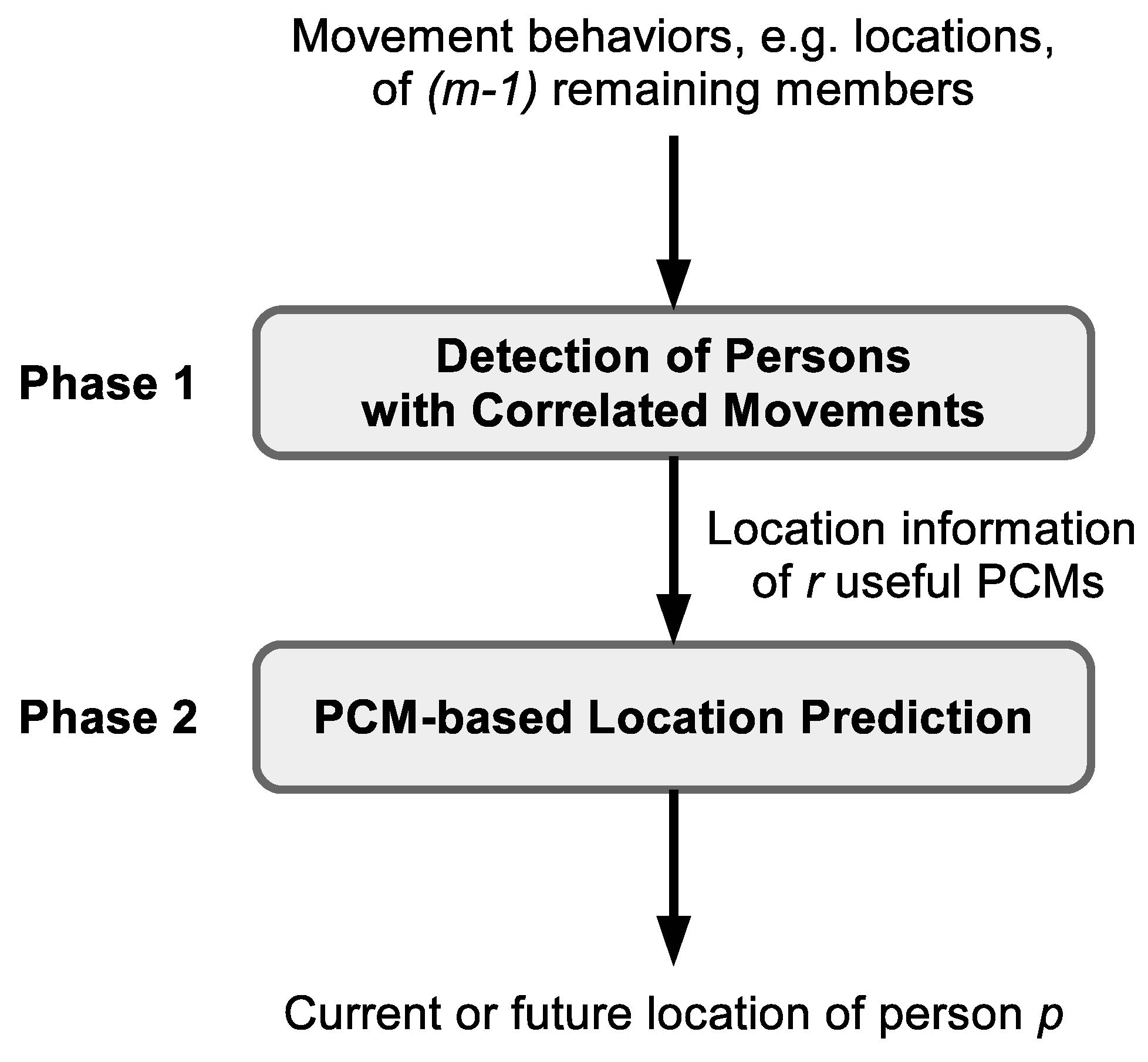
The proposed human mobility prediction framework consists of two phases, i.e., detection of persons with correlated movements (PCMs) and PCM-based location prediction, as shown in Figure 1. Let r denote the number of selected PCMs. In the first phase, r from among remaining members are extracted as PCMs of person p. Then, given the location information of the chosen members, the current or future position of person p is predicted.
In the first phase, we measure independently the social correlation between person p and each of the other members. In order to choose r useful PCMs for person p, these people are arranged according to their correlation scores, and r members with the highest scores are selected. The training set is used in the first phase where the input is vector that represents positional information of the remaining members. Table 2 shows an example of vector when the location of an arbitrary person, p, is estimated, where consists of spatial and temporal information. More specifically, , ,..., denotes the positions of the remaining members, while and account for the day and time slot indices, respectively. The first phase returns r PCMs of person p as the output.
Then, the location prediction phase estimates the most likely current or future position of person p using the spatio-temporal information of the r selected PCMs. Each sample of the training set is given by , where label is location information of person p at time t, and feature vector is spatio-temporal information of PCMs from time slots to where . In the proposed framework, a conditional probability distribution is estimated with the objective of maximizing probability . More specifically, given the location information of PCMs at time slots between and , the position of person p at time t needs to be predicted.
In this work, is considered, i.e., . In cases where , the location of PCMs in the previous time slot is used to predict the next location of person p (i.e., estimate person p’s future location at time t). Meanwhile, indicates that the model estimates the current position of the person using previous and current location information of PCMs. Whereas, if , the current position of the person is estimated given the information of PCMs at time t. Hereafter, the model is regarded as estimating the location of a person at time slot t. In the second phase, the PCM-based location prediction model is used to label an unknown sample as one out of possible locations.
There are several benefits from the proposed framework. Our model does not require a recent location sequence of person p when predicting the current or future location of person p, which is beneficial in cases where the location information of that person is not available. Note, however, that the location information of person p is necessary for training parameters of the prediction model.
The proposed framework first selects r PCMs based on human mobility characteristics, e.g., encounter frequency and behavioral patterns. Then, the location information of only these chosen PCMs is used to predict a person’s location at time t. As a result, by reducing redundant input features of the second phase, the overfitting problem can be mitigated. Moreover, the proposed framework allows for low time and space complexity.
5. Detection of Persons with Correlated Movements
In this section, two methods for selecting PCMs are proposed: community interaction similarity-based (CISB) and behavioral similarity-based (BSB) methods. Each uses a different measurement score to estimate the closeness between people’s movement patterns. Then, the r PCMs with the highest scores are selected.
5.1. Community Interaction Similarity-Based Method
Recall that the encounter frequency-based (EFB) method only uses direct encounters between certain individuals to estimate their friendship. In contrast, to measure correlation scores between persons p and q, CISB considers interactions between these persons and other community members as well as direct encounters between them. The CISB method is inspired by the fact that interactions and relationships with other members in the community have a great impact on a person’s behaviors.
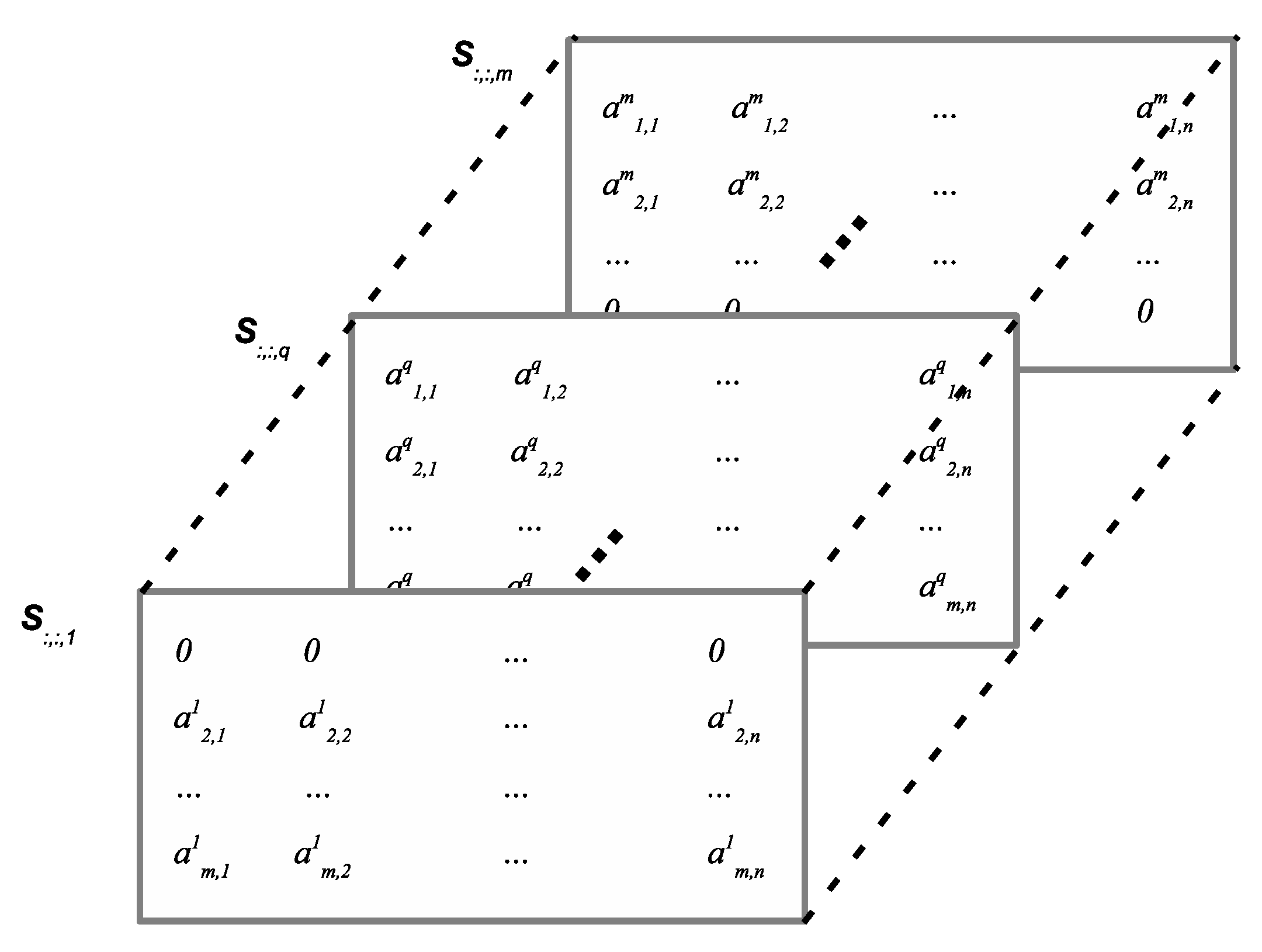
The CISB method utilizes the community interaction-based similarity (CIS) tensor shown in Figure 2, which represents the spatio-temporal encounters between people. The 3D CIS tensor, , consists of m layers each of which is a matrix, e.g., reflects the interactions between person q and the rest of the people. More specifically, the row in the matrix, i.e., , indicates the temporal encounters of persons p and q. Let and denote the total number of days in the overlapping period and the number of time slots per day, respectively. indicates the total number of samples per person during the whole period. accounts for the encounter between persons p and q in time slot t.
Vector , representing the encounters between persons p and q, is defined as follows:
Person p is not considered able to encounter himself or herself, because tensor represents the interactions between a person and the entire community, i.e., . The CIS tensor owns a symmetric property, i.e., .
From the CIS tensor, we reshape every 2D matrix, , to a one-dimensional vector with elements, which is denoted by . In order to evaluate the closeness between persons p and q, we consider the meet/min correlation coefficient [41] for measuring the similarity between and , which can be used if the vectors include a lot of 1 s. Thus, score between nodes p and q is calculated as follows:
where is the -norm of vector . After obtaining scores between person p and others, r people with the highest scores are chosen as PCMs.
Because of the characteristics of CIS, i.e., , and the dot product in the numerator of Equation (3), when measuring similarity , the interactions between persons p and q vanished unintentionally. For example, in calculating , two vectors and are as follows:
Since the first n elements of and the to elements of are zeros, similarity score that is estimated using Equation (3) does not consider the encounters of persons 1 and 2.
To avoid this vanishing problem, when calculating , the CIS tensor is temporarily modified as follows: and . For example, the modified vectors and corresponding to and , respectively, can be obtained as follows:
By using the modified CIS tensor, the CISB method takes into account the interactions with the entire community members.
5.2. Behavioral Similarity-Based Method
Persons p and q are said to have similar behavior if they experience a correlated visit behavior pattern, and hence, the location of a person can be estimated by using the other’s positional information. The places two people with similar behaviors visit at the same time are denoted as correlated locations. Note that correlated locations may be different. As seen in Table 3, persons p and q show a lot of similar behaviors even though they do not encounter each other. For example, person p exercises at a gym whenever person q visits a café. It is beneficial to measure the behavior similarity between persons because the location of a person can be inferred by using information of another person with a correlated behavioral pattern. For instance, the location of p at 3 p.m. on day 2 can be predicted using person q’s location (café). Based on this observation, in the BSB method, persons with the highest behavioral correlation are chosen as PCMs.
The key difference between the BSB method and friendship-based methods (i.e., CISB and EFB) is as follows. When selecting a PCM, the BSB method does not consider real friendships between people while friendship-based methods extract co-location information to measure the friendships between them. Specifically, in the EFB method, members with the highest number of encounters with a given person are chosen as PCMs. As shown in Table 3, persons p and u encounter each other several times (in math class and the laboratory), which indicates a close friendship between them. Therefore, in friendship-based methods, person u is likely to be chosen as a PCM of person p. Meanwhile, in case of two people with similar behaviors but different correlated locations, a person is not likely to be selected as a PCM of the other person. For example, persons p and q have the same behavior of having dinner at 5 p.m. at restaurant B and restaurant C, respectively. Since there is no encounter between people p and q, in friendship-based methods person q does not obtain a high enough score to be selected as a person p’s PCM. On the other hand, the BSB method considers this correlated behavior for choosing PCMs.
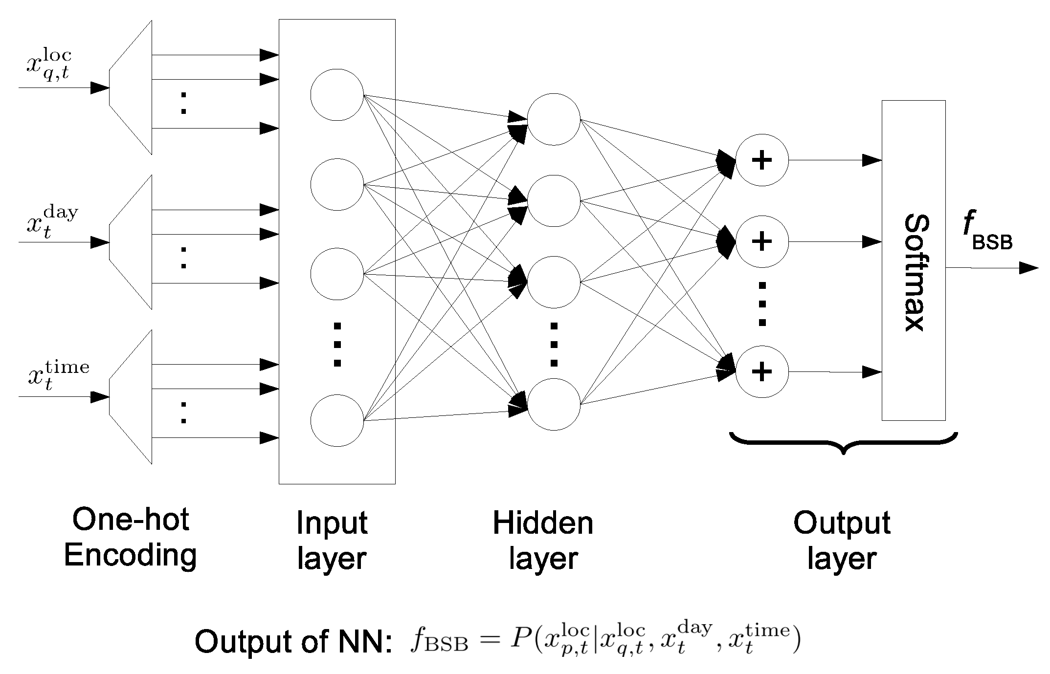
In the BSB method, a feed-forward neural network (NN), shown in Figure 3, is constructed to evaluate the behavioral similarity between persons p and q. is defined as the location of person q at time t, while and are indices of the day and the time slot at time t, respectively. The objective is to learn the underlying conditional probability distribution , i.e., the probability mass distribution that person p stays in a specific location during time slot t given the spatio-temporal information of person q.
Here, the training process is described. First, symbolic location is embedded into an -dimensional indicator vector using one-hot encoding, because there is no ordinal relationship between locations. Similarly, time slot and day indices (i.e., and , respectively) are also converted to indicator vectors. Then, these vectors are used as input units of the neural network including one hidden layer with 150 logistic sigmoid activation nodes. These input features propagate progressively throughout the network until reaching the softmax output layer, which obtains a conditional probability distribution over locations. is defined as the parameters of the NN consisting of weights, denoted by , and biases that are randomly initialized. Let denote the number of samples in the training dataset. After retrieving the conditional probability at the output layer, regularized cost function using cross-entropy error [42] is calculated as follows:
where and are the estimated output and target vectors of the instance, respectively. Note that is an element-wise operation. is the -based regularization term. The neural network model is trained to minimize cost function using a back-propagation algorithm combined with a gradient descent method.
In order to select r PCMs of person p, NNs are trained separately, where each NN measures the similar behavior pattern between individuals p and q (). The prediction accuracy, , of the NN, which indicates the behavioral similarity of persons p and q, is defined as the ratio of the number of correctly predicted instances to the number of test samples. In the BSB method, r PCMs among the remaining members with the highest are selected.
It is worthwhile to note that there are alternative ways of selecting a set of PCMs. For example, forward search (FS) [43] begins with an empty set and then progressively incorporates each feature (i.e., PCM) into the set. However, FS has an inherent weakness, i.e., high time and space complexity when a large number of features need to be selected.
Another simple approach that can be considered is that positional information of all remaining people is used as input features for a prediction model that labels the location of a person at time t with one of the positions. In our work, this simple method is called ignored feature selection (IFS) since there is no feature selection process. Note that IFS may need to train a model with tens or hundreds of thousands of features, which may result in a long training time, and might suffer from the overfitting problem.
In order to gain insight into computational costs, the number of training parameters for three methods including IFS, FS, and BSB is compared. For IFS, there is no PCM selection phase, i.e., the location of person p is predicted given the positional information of the other people. With FS, to choose the first PCM, NNs are trained independently. To select the second PCM, a combination of the first PCM and one of the remaining members is examined; NNs need to be learned, each of which estimates person p’s location at time slot t given the contextual information of two examined people. Similarly, to select the PCM, NNs are used to evaluate the subset of the already selected PCMs and one of the remaining members. In the FS method, a large r value leads to a significant increase in the number of training parameters.
In the BSB and FS methods, it is assumed that three selected PCMs are used for the location prediction phase, where a neural network with three hidden layers of 500, 150, and 50 neurons is considered. For a fair comparison, the number of hidden neurons for IFS is proportional to that of the BSB/FS methods in the mobility prediction phase with the ratio because and r are the numbers of people whose location information is given to the IFS and BSB/FS methods, respectively.
Table 4 compares the number of training parameters of the three methods, where , , and denote the number of parameters, i.e., weights and biases, in behavioral similarity-based, ignored feature selection, and forward search methods, respectively. When the total number of people, m, increases, the three considered methods need to train more parameters. However, the BSB method always learns the least number of parameters. Moreover, the increase rate is quite different in each method, e.g., when m varies from 43 to 1000 people, rises times, compared to times with and times with . In summary, because only location information of PCMs is used to predict human mobility of a given person, the proposed BSB method incurs a much lower computation cost in terms of time and space complexity than IFS and FS, which makes the BSB method more practical, particularly when there is a large number of people.
6. The PCM-Based Location Prediction (PLP) Model
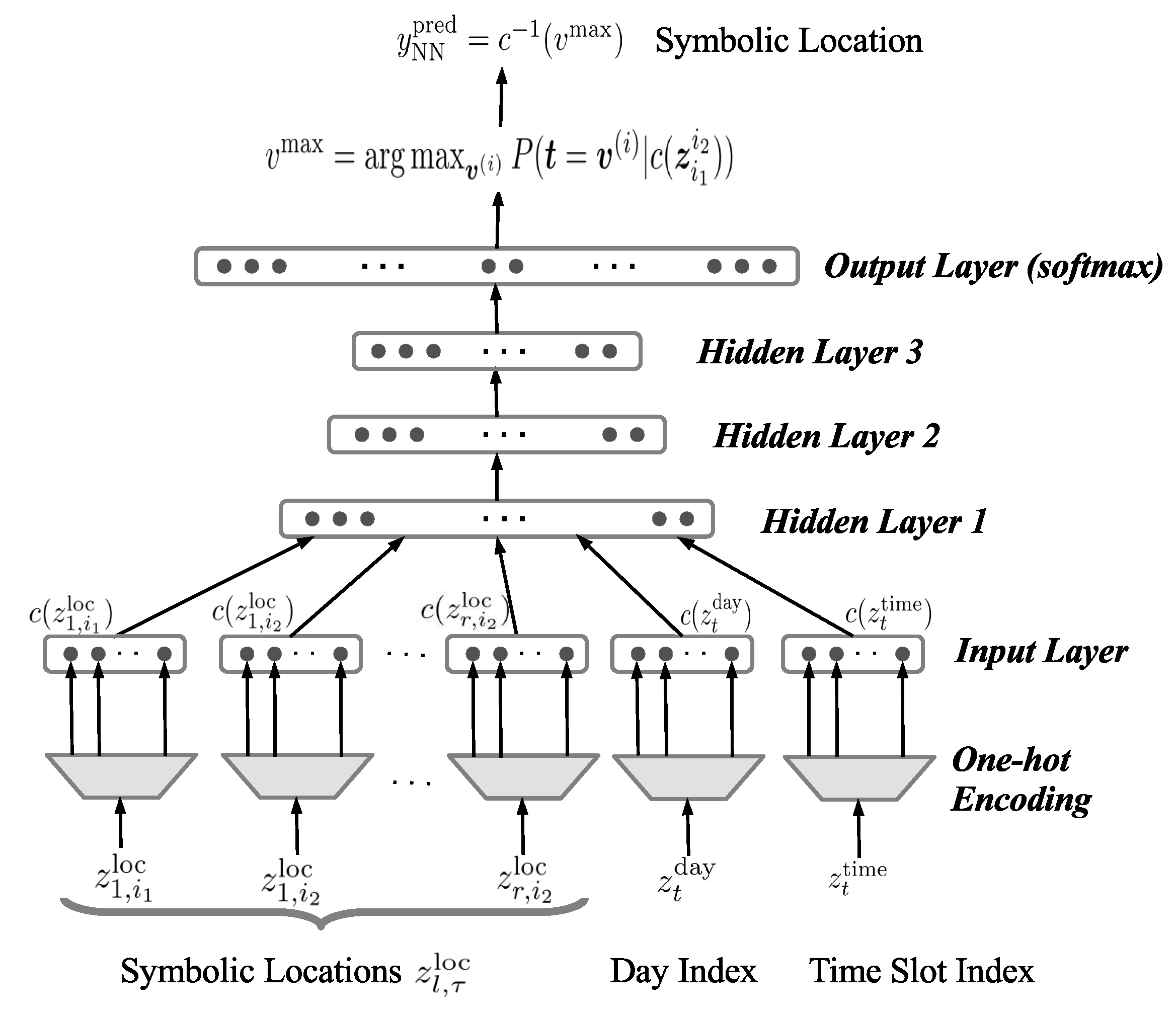
In this section, we propose the PCM-based location prediction (PLP) model based on the neural network to predict human mobility given the movement patterns of r selected PCMs. Figure 4 illustrates the NN-based prediction model where the location of a person at time t is estimated given the information of r PCMs, i.e., . Spatial information , where and , indicates the symbolic location of the r PCMs from time to . Meanwhile, temporal information and are the indices of the day of the week and the time slot in the day at time t, respectively. Let denote the output of the NN-based predictor, i.e., the most likely location of the person during time slot t. Note that to predict the location at time t of m persons in the community, m corresponding NN-based prediction models need to be trained separately. The remainder of this subsection describes an NN-based predictor.
The function can be decomposed into three parts, as follows.
- The contextual information of r PCMs, i.e., , is mapped onto real vectors using the one-hot encoding function , where output is the indicator vector in which only one element is set to 1 while others are 0. Since is the size of the extracted location set, are vectors in , where is a set of binary numbers; is a day-index vector in . Meanwhile, the cellular trace between 8 a.m. and 12 p.m. is extracted and each time slot lasts 30 min; therefore, is mapped onto a 32-dimensional binary vector. In addition, grouped time slots are considered. In this case, is a three-dimensional vector where each dimension corresponds to one of the three parts of a day, i.e., morning, afternoon, and evening.
- The NN classifier maps input sequence to a conditional probability distribution over locations. Let denote an indicator vector in which only the element is 1 and others are 0 (). Vector is defined as the target vector of the NN classifier. The output of the NN is denoted by vector where the element, , estimates posterior probability that the person stays in location i given the information of r PCMs.
- The vector that indicates the most likely location of the person is mapped onto symbolic position by the inverse function, i.e., .
Now, the neural network training process that includes feed-forward propagation, a cost function calculation, and a parameter update is presented. First, feed-forward propagation is described. In this work, is defined as the number of hidden layers, and a neural network is considered with logistic sigmoid activation units denoted by . Hereafter, the input layer is referred to as layer 0, the hidden layer as layer j (), and the output layer as layer . Let denote all learning parameters consisting of weights and biases of the NN classifier. More specifically, and are the matrix of weights and the vector of biases, respectively, that indicate connections from layers to j; is defined as the state vector at layer j, and is given by:
Note that is a vector of input features at layer 0. For the output layer, the unnormalized output vector is calculated by .
Then, the output of a softmax function represents the categorical distribution over locations where the element of the output vector reflecting the probability that the person stays at time t in location i is calculated as follows:
where is the value of unnormalized output vector .
Secondly, the calculation of the cost function is briefly described below. Assume that there are training instances. Cost function using the cross entropy metric and regularization method can be expressed as follows:
where and are, respectively, the estimated output and target vectors of the instance, and denotes the weight matrices. Note that is an element-wise operation. Regularization is implemented using the parameter norm penalty.
Finally, parameters including weights and biases are obtained by applying a back propagation algorithm, which minimizes the cost value using the gradient descent method with momentum. Let and denote the learning rate of gradient descent and the momentum coefficient, respectively, (). Let denote a training parameter in the set , i.e., . Then, each is updated in the epoch as follows:
where partial derivative is the gradient of the cost function with respect to , and is the current velocity vector with the same dimensions as parameter .
7. Evaluation Results and Discussion
In this section, the performance of the human mobility prediction framework is examined under different PCMs detection methods and is compared with the baseline prediction model, most frequent location (MFL). The whole dataset is randomly partitioned into training, validation, and test sets at the ratio of 5:2:3. Recall that in case of the Dartmouth dataset the 118-day period is selected and for each day human mobility from 8 h to 24 h is considered. Since each time slot lasts 30 min, there are total 32 time slots per day. Therefore, the number of samples in the Dartmouth dataset is . The training, validation, and test sets consist of 1886; 755; and 1133 instances, respectively. The training set is used to fit the model while the purpose of validation set is to determine the appropriate hyper-parameters for the neural network, e.g., the number of hidden layers, hidden units, activation units, and learning rate. Note that only the training set is used in the first phase of the prediction model and the performance of model is estimated based on the test set.
Table 5 presents the setup for the mobility prediction framework. Specifically, the two proposed PCM selection methods consisting of community interaction similarity-based (CISB) and behavioral similarity-based (BSB) are evaluated and compared with three recent selection approaches: encounter frequency-based method (EFB) [18,23,24], spatial closeness (SC) [6], and spatiotemporal closeness (STC) [6]. Table 6 shows a list of acronyms which are used in the manuscript.
Recall that Alhasoun et al. [6] constructed a prediction model based on dynamic Bayesian networks which leveraged historical location data of selected PCMs to predict the most probable position of the person-of-interest. However, the prediction model in [6] requires to know the last visited place of the person-of-interest, which is not applicable to our considering problem where the historical position data of the person-of-interest is assumed to be unknown. Note that since there was no existing prediction model designed for the considering problem, the PCM-based location prediction (PLP) model is used in the experiments.
Additionally, we make a performance comparison between our two proposed PCMs selection approaches and counterpart methods in [6]. There were three similarity measurement metrics to select PCMs in [6], and specifically the first method, temporal closeness, compares patterns of communication (e.g., call, sms, and data) between people. Due to the requirement of extra communication information of members, the temporal closeness is not considered as a counterpart method for selecting PCMs in our work. Therefore, we compare the proposed PCMs selection methods with only two approaches in [6]: STC and SC.
For the PLP model, a variety of NN architectures which have a different number of layers, hidden units, and activation functions were examined. Then, among the considered setting, the most appropriate NN architecture was selected by using the validation set. Specifically, there is 1 hidden layer of 150 sigmoid activation units in the NN of the BSB approach. In the NN-based predictor, 500, 150, and 50 sigmoid hidden units are used in the first, second, and third hidden layers, respectively. Weight and bias values are initialized with normal distribution. The regularization coefficient is set to 0.01. Learning rate in the gradient descent and the momentum coefficient are set to 0.4 and 0.1, respectively. Full batch learning with 1500 iterations is examined. Note that only the training set is used to select the r PCMs in the first phase of the prediction models. For example, in case of the Dartmouth dataset, r PCMs are determined by using the training set of 1866 samples which are randomly selected from the total 3776 instances.
Moreover, three types of temporal information are considered. The number of selected PCMs varies from 1 to 5, while top-k accuracy is considered with . In addition, un-grouped and grouped time slot features are compared. The bold text in the second column of Table 5 denotes default values of the prediction model. In this work, performance metrics including average and standard deviation of prediction accuracy are obtained over 5 runs. The results are collected via averaging the entire people.
The most noticeable results are summarized as follows. From the conducted experiments, the performance of designed PLP model outperforms that of the baseline method, MFL. With regard to the PCMs selection methods, the proposed BSB shows significantly better performance than other PCM extraction approaches. In addition, the generalization capability of the proposed framework increases as a larger number of PCMs are embedded into the model. In particular, this increase is more clearly shown in case of BSB.
7.1. Performance Comparison of PCM Selection Methods
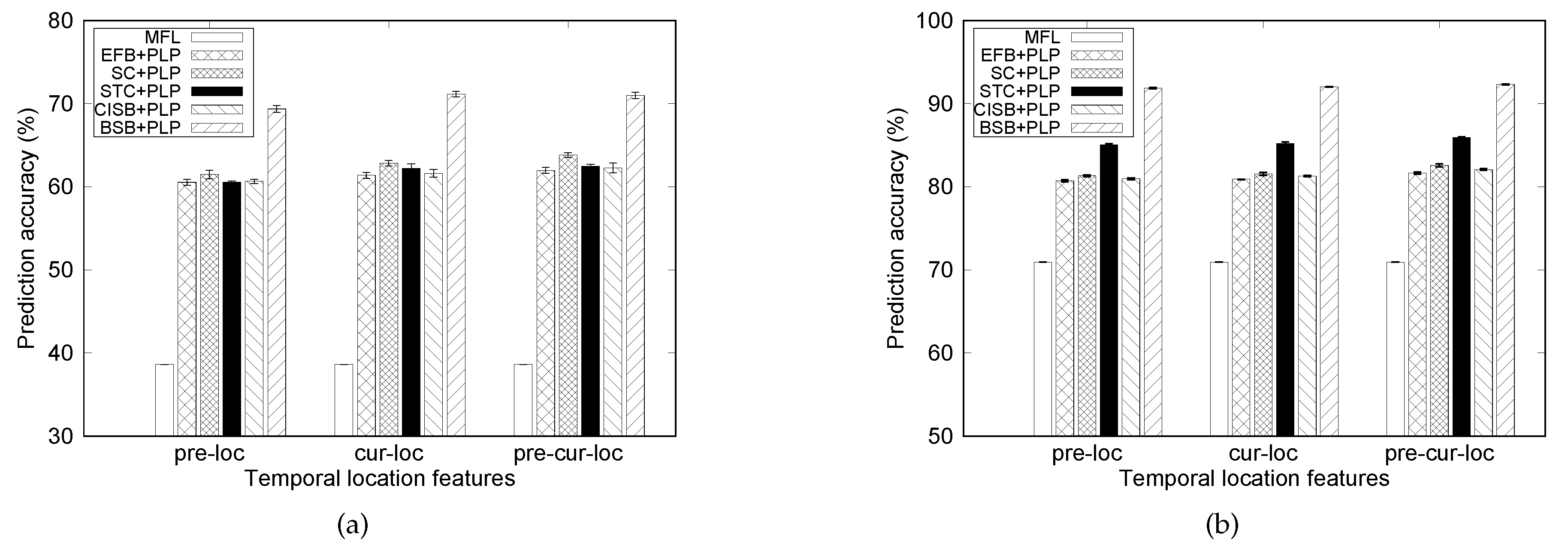
In this subsection, the performance results of PCMs extraction methods are discussed with different temporal features of selected PCMs. The location of a person during time t is predicted with the support of PCMs’ positions during the time slot (denoted by pre-loc), time slot t (denoted by cur-loc), and both and t time slots (denoted by pre-cur-loc). Recall that the time slot lasts 15 min. The obtained results are shown in Figure 5.
First, we evaluate the predictability of the baseline prediction model, most frequent location (MFL). As can be seen in Figure 5, the MFL model achieves much lower performance than the proposed PLP architecture, and specifically leads to top-1 accuracy of 38.62% and 70.92% with MIT and Dartmouth datasets, respectively. Since the MFL model does not use information of PCMs to predict where person p stays at time t, the temporal feature of PCMs does not affect the performance of MFL model.
Now, the performance of PLP model is analyzed with different PCM selection methods. In EFB and CISB methods, members with the most similar movement paths are selected as PCMs, i.e., people who stay the most frequently with a given person. The main difference between these two methods is that the EFB scheme weights the link of two people based on direct encounters between them, whereas the CISB method compares community interactions between persons to estimate their social correlation. Even though in some cases the CISB method obtains slightly higher accuracy than the EFB method, the two generally achieve similar performance. This indicates that a social relationship between two persons can be mainly reflected by direct interactions between them.
In contrast, the BSB method aims at selecting PCMs with the most correlated behavioral patterns. Our work shows that discovering behavior patterns helps to significantly improve prediction accuracy of the model compared to the friendship-based method. In fact, for members who work in the same university or company, they tend to have similar lifestyles (e.g., behavioral pattern) owing to the common schedules of the workplace. Therefore, considering behavioral similarity between people can be helpful in selecting better PCMs for predicting people’s locations. Specifically, when embedding pre-cur-loc information of PCMs selected by the BSB scheme into the PLP model, we achieve top-1 prediction accuracy as high as 71.00% and 92.31%, respectively, with MIT and Dartmouth datasets.
In the SC scheme, regardless of encounters between two people, members who have similar spatial distribution, or longevity of visiting places are selected as PCMs. The SC method may choose PCMs who have different frequency or regularity of staying in locations with the person-of-interest. For example, if two people p and q spend 4 h at the library everyday, the SC method is likely to choose person q as a PCM of p. However, if person p stays at the library in the whole afternoon while q spends 2 h in the morning and 2 h in the evening, using location information of q may not be appropriate to predict the mobility of person p.
Meanwhile, in case of the STC method, two people have a high closeness score if they move in a synchronous manner or their movement are highly dependent. Note that PCMs in both STC and BSB tend to move in a synchronous way with the person-of-interest. However, a fundamental difference between BSB and STC is that the STC method does not consider the temporal information when measuring the similarity between two people. Specifically, the STC approach computes the spatial distribution of person p given the location of person q. Meanwhile, the BSB method investigates the spatial distribution of person p given both spatial and temporal information of person q. By considering the temporal data when selecting PCMs, the BSB approach is able to measure movement association with both spatial and temporal aspects. As a consequence, the BSB method achieves significantly higher prediction accuracy than the STC one with both datasets.
However, the performance gap between BSB and STC in the Dartmouth traces is noticeably smaller than that in the MIT one. The gap difference may come from different characteristics of human mobility in two datasets. Recall that the STC scheme does not consider the dependence between human movement and the temporal information. Therefore, if human mobility extracted from a dataset (e.g., the Dartmouth) is not highly related to the temporal data, the STC can achieve better accuracy than the case of strong relationship between human movement and the temporal information.
One should note that BSB, SC and STC approaches do not take into account the actual encounter or friendship between people. The experiment results in Figure 5 indicate that friendship-based methods (EFB and CISB) causes the lower performance than other approaches (BSB, SC, and STC) in which friendship is not considered. In addition, the proposed BSB approach achieves the most accurate prediction among the considered PCMs selection methods. For example, using location data of PCMs at time and t, the PLP model predicts human locations at time t with top-1 accuracy of 81.64%, 82.57%, 85.92%, 82.07%, and 92.31% using EFB, SC, STC, CISB, and BSB methods, respectively, in case of the Dartmouth dataset.
Also, from the observations in Figure 5, among three considered temporal features, pre-cur-loc and cur-loc lead to quite similar performance in both datasets. For example, in case of the MIT traces, the PLP model achieves 71.13% and 71.00% accuracy in predicting the location of person p given pre-cur-loc and cur-loc information of PCMs, respectively. As anticipated, using data of PCMs during time t (cur-loc) can result in a more accurate prediction than the use of (pre-loc).
7.2. Top-k Accuracy
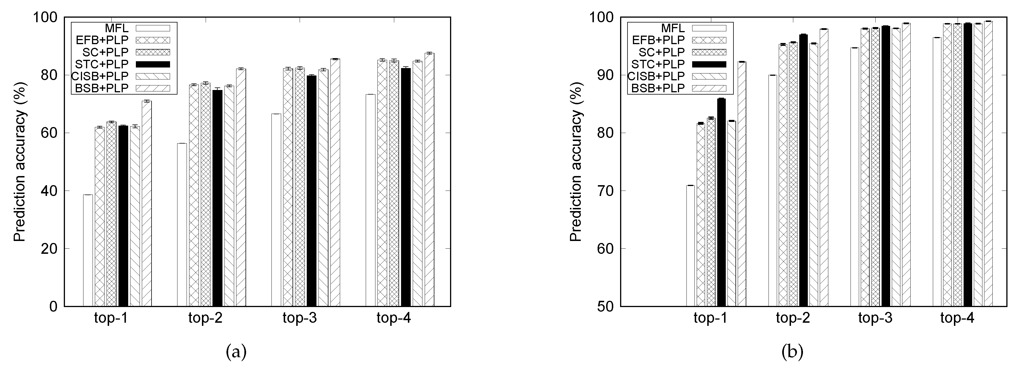
In this subsection, we evaluate the top-k accuracy of the proposed PLP model when . Other parameters are set to the default values shown in Table 5. For top-k accuracy, the model outputs a list of k location(s) with the highest probability. If the correct location belongs to the list of k element(s), the prediction is considered accurate.
As expected, Figure 6 shows that the obtained accuracy increases from top-1 to top-4. For example, in case of the MIT dataset, the BSB approach results in 71.00%, 82.17%, 85.53%, and 87.59% accuracy corresponding to top-1, top-2, top-3, and top-4, respectively. In all examined PCM selection schemes, the steepest rising rate is observed when k changes from 1 to 2. Then, the outcomes tend to plateau.
As can also be observed from Figure 6, there is higher prediction accuracy in the Dartmouth dataset than the MIT one. This observation is attributed to the fact that human movement in the MIT dataset was collected within a wider area than that in the Dartmouth traces. More specifically, all APs in the Dartmouth dataset are located in the university campus while movement trajectories of people in the MIT dataset are not bounded in the school area. Therefore, people mobility in the MIT dataset tends to be more divergent and more difficult to predict than that in the Dartmouth traces.
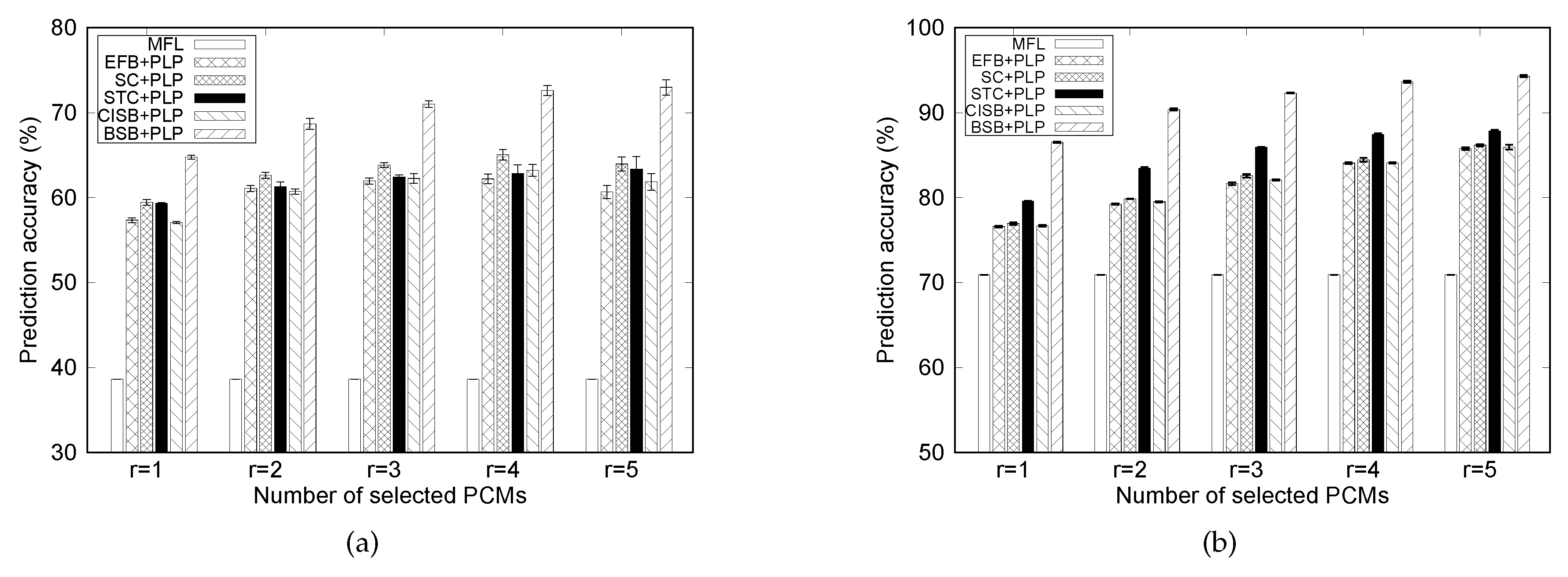
7.3. Effects of the Number of PCMs
In this subsection, the number of selected PCMs varies from 1 to 5. As seen in Figure 7b, using location information of one PCM (i.e., ), the PLP model obtains top-1 accuracy of 86.53% with the BSB method compared with 70.92% in case of the MFL model. Meanwhile, the PLP model with EFB, SC, STC, and CISB approaches results in 76.58%, 76.94%, 79.57%, and 76.70% accuracy, respectively.
It should be emphasized that when adding more PCMs, the performance of the prediction model is generally enhanced. In friendship-based methods (CISB and EFB), this is attributed to the fact that a person usually interacts with multiple PCMs rather than one person during the day. For example, in the morning, person p encounters co-worker q at the workplace. At lunch, p and r have an appointment at their favorite restaurant. Then, persons p and s go to the fitness center to exercise in the afternoon. In other PCMs selection approaches, the performance gain with more PCMs is due to the fact that a person has movement correlation with various PCMs depending on the time of a day. For instance, assume that person p is a middle-aged man. He may have a similar behavioral pattern with younger co-worker q during the daytime, whereas after work, he may have behaviors similar to other middle-aged men, rather than with the younger co-workers.
Moreover, the performance gap between the BSB and friendship-based methods (CISB and EFB) becomes larger as the number of PCMs embedded in the model increases especially in the MIT dataset. This is because selected PCMs of CISB and EFB tend to have more similar encounter patterns with person p than under the BSB method. To show this, KL divergence [44] is considered to measure similarity between temporal encounter distributions of PCMs and person p. Vector denotes the probability distribution of encounters between persons p and q. The element of represents the probability that persons p and q encounter each other during time slot i. Vector indicates a distribution of encounters between persons p and r. The length of and equals the number of samples for each person. Using KL divergence, the difference between the two probability distributions is given by:
where and are the elements of vectors and , respectively. If the score from KL divergence is small, encounter distributions between PCMs and person p are close, which indicates similar movement patterns between PCMs.
Assume that a mobility prediction model with r PCMs is considered. If another PCM with highly similar movement patterns to those of the r existing PCMs is added at input, the location information of the added PCM would not be helpful in predicting location of person p. As shown in Table 7, in cases where the number of selected PCMs is 5, the average value of KL divergence between PCMs’ patterns of encounters with a person-of-interest is 11.01, 11.03, and 15.19 in EFB, CISB, and BSB methods, respectively. We can also observe from Table 7 that KL divergence values of SC and STC approaches are generally higher than friendship-based ones since SC and STC do not consider encounters between people.
Lower KL divergence values from EFB and CISB methods indicate that they tend to select PCMs with more similar mobility patterns than the BSB method, and accordingly, movement patterns of the selected PCMs under the BSB method are more divergent than those under EFB/CISB methods. This contributes to a large accuracy gap between the BSB and friendship-based methods. The results also agree with the assumption that correlated locations in the BSB method do not have to be the same places.
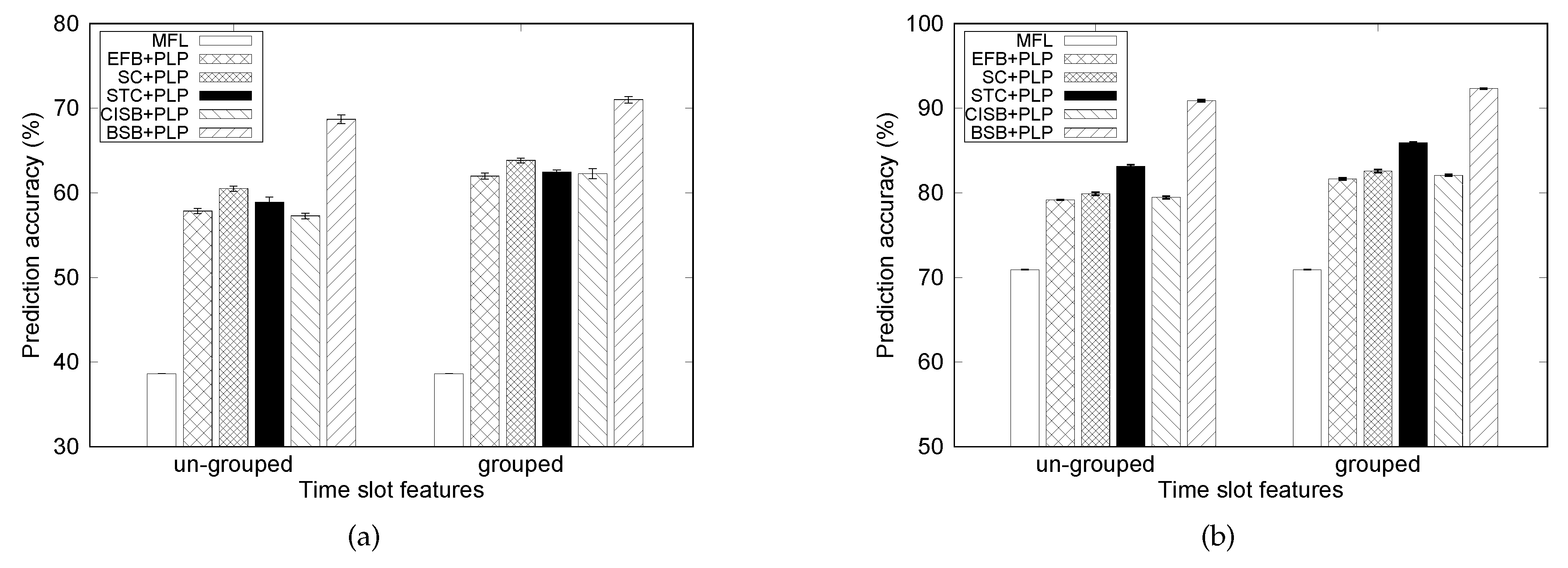
7.4. Effects of Time Slot Feature Selection
Figure 8 compares the precision of the mobility prediction model with two different time slot features: un-grouped and grouped. For the un-grouped case, 32 time slots in a day are mapped into a 32-dimensional vector. Meanwhile, for the grouped case, one-hot encoding converts a time slot index into a vector in where each dimension indicates one of the three parts of a day.
In addition, as shown in Figure 8, it is clear that grouping time slot feature achieves higher prediction accuracy than with un-grouped features. The results reflect that people tend to spend time with each other for a relatively long period. This becomes more understandable in environments like university campuses or companies, where people usually stay with their colleagues for a significant amount of time during the day. After work, they may enjoy leisure activities with friends in the evening. Another reason for the low performance with the un-grouped case may be the small number of data samples compared with the large input dimensions in the un-grouped case.
8. Concluding Remarks
Human mobility prediction has been a key point for the success of a variety of potential applications. For instance, with the development of device-to-device communication technologies, being able to accurately predict human locations will facilitate the design of an efficient data routing protocol in opportunistic networks. Moreover, the location prediction model inspires further applications such as urban data mining, location-based recommendation services, and contagious disease control. In addition, location estimation is required even when someone may not be willing to share their locations (e.g., geographic profiling of criminals).
Therefore, in this work, we address the mobility prediction problem in which the current or next location of a person is estimated, especially without requiring the positional history of that person. Since the movement of a person is highly related to other people, a two-phase framework is proposed in which persons with correlated movements (PCMs) with the person-of-interest are determined in the first phase. Then, information of these selected PCMs is leveraged in the second phase to estimate the location of the person-of-interest. For selecting PCMs, the communication interaction similarity-based (CISB) method considers encounter interactions between people, whereas the behavioral similarity-based (BSB) scheme selects PCMs who have similar behavioral patterns, instead of considering co-location between people.
For the considered problem, our approach is robust, because it can reduce overfitting by only using the location information of the selected PCMs to estimate the positions of the person-of-interest. Low time and space computational complexity is also achieved. Furthermore, geographic locations are not required in our model. Experimental results show that the BSB method gains significant improvement over other PCMs extraction approaches. In addition, the performance generally increases when more PCMs were embedded into the designed prediction model. In particular, a large number of PCMs is more beneficial under the BSB method than others.
However, our PCMs selection methods are centralized approaches because of requiring mobility traces of all people. Therefore, the proposed PCMs extraction methods are restricted to small or medium networks. In addition, information assurance needs to be taken into account since mobility data of people is exchanged in the network. As a future work, to address the limitations of the centralized approaches, we plan to design a PCMs extraction method which does not require mobility traces of all people. Furthermore, datasets with more people will be used to examine the proposed prediction model in the future work.
Author Contributions
S.Y. and T.-N.D. designed the framework. The performance evaluation was conducted by T.-N.D. and D.V.L. All authors have written and approved the manuscript.
Funding
This research was supported by the Basic Science Research Program through the National Research Foundation of Korea (NRF) funded by the Ministry of Education (NRF-2016R1D1A3B03934617).
Conflicts of Interest
The authors declare no conflict of interest.
References
- Asgari, F.; Gauthier, V.; Becker, M. A survey on Human Mobility and its applications. arXiv, 2013; arXiv:1307.0814. [Google Scholar]
- Noulas, A.; Scellato, S.; Lathia, N.; Mascolo, C. Mining User Mobility Features for Next Place Prediction in Location-Based Services. In Proceedings of the 2012 IEEE 12th International Conference on Data Mining, Brussels, Belgium, 10–13 December 2012; pp. 1038–1043. [Google Scholar]
- Su, J.; Chin, A.; Popivanova, A.; Goel, A.; de Lara, E. User mobility for opportunistic ad-hoc networking. In Proceedings of the Sixth IEEE Workshop on Mobile Computing Systems and Applications, Washington, DC, USA, 3 December 2004; pp. 41–50. [Google Scholar]
- Wesolowski, A.; Eagle, N.; Tatem, A.J.; Smith, D.L.; Noor, A.M.; Snow, R.W.; Buckee, C.O. Quantifying the Impact of Human Mobility on Malaria. Science 2012, 338, 267–270. [Google Scholar] [CrossRef] [PubMed] [Green Version]
- Rossmo, D. Geographic Profiling; CRC Press: Boca Raton, FL, USA, 1999. [Google Scholar]
- Alhasoun, F.; Alhazzani, M.; Aleissa, F.; Alnasser, R.; González, F. City Scale Next Place Prediction from Sparse Data through Similar Strangers. In Proceedings of the ACM KDD Workshop, Halifax, NS, Canada, 14 August 2017. [Google Scholar]
- Zhao, Z.; Koutsopoulos, H.N.; Zhao, J. Individual mobility prediction using transit smart card data. Transp. Res. Part C Emerg. Technol. 2018, 89, 19–34. [Google Scholar] [CrossRef]
- Cho, E.; Myers, S.A.; Leskovec, J. Friendship and Mobility: User Movement in Location-based Social Networks. In Proceedings of the 17th ACM SIGKDD International Conference on Knowledge Discovery and Data Mining, San Diego, CA, USA, 21–24 August 2011; pp. 1082–1090. [Google Scholar]
- Sadilek, A.; Kautz, H.; Bigham, J.P. Finding Your Friends and Following Them to Where You Are. In Proceedings of the Fifth ACM International Conference on Web Search and Data Mining, Marina Del Rey, CA, USA, 8–12 February 2012; pp. 723–732. [Google Scholar]
- Zhang, D.; Zhang, D.; Xiong, H.; Yang, L.T.; Gauthier, V. NextCell: Predicting Location Using Social Interplay from Cell Phone Traces. IEEE Trans. Comput. 2015, 64, 452–463. [Google Scholar] [CrossRef]
- Bengio, Y.; Ducharme, R.; Vincent, P.; Janvin, C. A Neural Probabilistic Language Model. J. Mach. Learn. Res. 2003, 3, 1137–1155. [Google Scholar]
- Eagle, N.; Pentland, A. Reality Mining: Sensing Complex Social Systems. Pers. Ubiquitous Comput. 2006, 10, 255–268. [Google Scholar] [CrossRef]
- Rappaport, T.S.; Roh, W.; Cheun, K. Mobile’s millimeter-wave makeover. IEEE Spectr. 2014, 51, 34–58. [Google Scholar] [CrossRef]
- Zeng, W.; Fu, C.W.; Arisona, S.M.; Schubiger, S.; Burkhard, R.; Ma, K.L. A visual analytics design for studying rhythm patterns from human daily movement data. Vis. Inform. 2017, 1, 81–91. [Google Scholar] [CrossRef]
- Jedari, B.; Liu, L.; Qiu, T.; Rahim, A.; Xia, F. A Game-theoretic Incentive Scheme for Social-aware Routing in Selfish Mobile Social Networks. Future Gener. Comput. Syst. 2017, 70, 178–190. [Google Scholar] [CrossRef]
- Zhang, X.; Cao, G. Transient Community Detection and Its Application to Data Forwarding in Delay Tolerant Networks. IEEE/ACM Trans. Netw. 2017, 25, 2829–2843. [Google Scholar] [CrossRef]
- Mo, T.; Sen, S.; Lim, L.; Misra, A.; Balan, R.K.; Lee, Y. Cloud-Based Query Evaluation for Energy-Efficient Mobile Sensing. In Proceedings of the 2014 IEEE 15th International Conference on Mobile Data Management, Brisbane, Australia, 14–18 July 2014; Volume 1, pp. 221–224. [Google Scholar]
- Cao, L.; She, J. Can Your Friends Predict Where You Will Be? In Proceedings of the 2014 IEEE International Conference on Internet of Things (iThings), and IEEE Green Computing and Communications (GreenCom) and IEEE Cyber, Physical and Social Computing (CPSCom), Taipei, Taiwan, 1–3 September 2014; pp. 450–455. [Google Scholar]
- Kotz, D.; Henderson, T.; Abyzov, I.; Yeo, J. CRAWDAD Dataset Dartmouth/campus (v. 2009-09-09), 2009. Available online: http://crawdad.cs.dartmouth.edu/dartmouth/campus (accessed on 3 January 2019).
- Karamat Jahromi, K.; Zignani, M.; Gaito, S.; Rossi, G.P. Predicting Encounter and Colocation Events. Ad Hoc Netw. 2017, 62, 11–21. [Google Scholar] [CrossRef]
- Nunes, I.O.; Celes, C.; de Melo, P.O.V.; Loureiro, A.A. GROUPS-NET: Group meetings aware routing in multi-hop D2D networks. Comput. Netw. 2017, 127, 94–108. [Google Scholar] [CrossRef] [Green Version]
- Shi, Y.; Chen, S.; Xu, X. MAGA: A Mobility-Aware Computation Offloading Decision for Distributed Mobile Cloud Computing. IEEE Internet Things J. 2018, 5, 164–174. [Google Scholar] [CrossRef]
- Bulut, E.; Szymanski, B.K. Exploiting Friendship Relations for Efficient Routing in Mobile Social Networks. IEEE Trans. Parallel Distrib. Syst. 2012, 23, 2254–2265. [Google Scholar] [CrossRef]
- Nguyen, C.; Yoon, S.; Kim, Y. Discovering Social Community Structures Based on Human Mobility Traces. Mob. Inf. Syst. 2017, 2017, 2190310. [Google Scholar] [CrossRef]
- Noulas, A.; Scellato, S.; Lambiotte, R.; Pontil, M.; Mascolo, C. A tale of many cities: Universal patterns in human urban mobility. PLoS ONE 2012, 7, e37027. [Google Scholar] [CrossRef]
- Gonzalez, M.C.; Hidalgo, C.A.; Barabasi, A.L. Understanding individual human mobility patterns. Nature 2008, 453, 779–782. [Google Scholar] [CrossRef] [PubMed]
- Karamshuk, D.; Boldrini, C.; Conti, M.; Passarella, A. Human mobility models for opportunistic networks. IEEE Commun. Mag. 2011, 49, 157–165. [Google Scholar] [CrossRef]
- Crandall, D.J.; Backstrom, L.; Cosley, D.; Suri, S.; Huttenlocher, D.P.; Kleinberg, J.M. Inferring social ties from geographic coincidences. Proc. Natl. Acad. Sci. USA 2010, 107, 22436–22441. [Google Scholar] [CrossRef] [Green Version]
- Pang, H.; Wang, P.; Gao, L.; Tang, M.; Huang, J.; Sun, L. Crowdsourced mobility prediction based on spatio-temporal contexts. In Proceedings of the 2016 IEEE International Conference on Communications (ICC), Kuala Lumpur, Malaysia, 23–27 May 2016; pp. 1–6. [Google Scholar]
- Mathew, W.; Raposo, R.; Martins, B. Predicting Future Locations with Hidden Markov Models. In Proceedings of the 2012 ACM Conference on Ubiquitous Computing, Pittsburgh, PA, USA, 5–8 September 2012; pp. 911–918. [Google Scholar]
- Eagle, N.; Clauset, A.; Quinn, J.A. Location Segmentation, Inference and Prediction for Anticipatory Computing. In Proceedings of the AAAI Spring Symposium: Technosocial Predictive Analytics, London, UK, 23–26 March 2009; pp. 20–25. [Google Scholar]
- Zeng, S.; Wang, H.; Li, Y.; Jin, D. Predictability and Prediction of Human Mobility Based on Application-Collected Location Data. In Proceedings of the 2017 IEEE 14th International Conference on Mobile Ad Hoc and Sensor Systems (MASS), Chengdu, China, 9–12 October 2017; pp. 28–36. [Google Scholar]
- Backstrom, L.; Sun, E.; Marlow, C. Find Me if You Can: Improving Geographical Prediction with Social and Spatial Proximity. In Proceedings of the 19th International Conference on World Wide Web, Raleigh, NC, USA, 26–30 April 2010; pp. 61–70. [Google Scholar]
- Hossmann, T.; Spyropoulos, T.; Legendre, F. Putting Contacts into Context: Mobility Modeling Beyond Inter-contact Times. In Proceedings of the Twelfth ACM International Symposium on Mobile Ad Hoc Networking and Computing (MobiHoc ’11), Paris, France, 16–20 May 2011; ACM: New York, NY, USA, 2011. [Google Scholar]
- Su, Y.; Li, X.; Tang, W.; Xiang, J.; He, Y. Next Check-in Location Prediction via Footprints and Friendship on Location-Based Social Networks. In Proceedings of the 2018 19th IEEE International Conference on Mobile Data Management (MDM), Aalborg, Denmark, 26–28 June 2018; pp. 251–256. [Google Scholar]
- Sepahkar, M.; Khayyambashi, M.R. A novel collaborative approach for location prediction in mobile networks. Wirel. Netw. 2018, 24, 283–294. [Google Scholar] [CrossRef]
- Girvan, M.; Newman, M.E.J. Community structure in social and biological networks. Proc. Natl. Acad. Sci. USA 2002, 99, 7821–7826. [Google Scholar] [CrossRef] [PubMed] [Green Version]
- Boston, D.; Mardenfeld, S.; Pan, J.S.; Jones, Q.; Iamnitchi, A.; Borcea, C. Leveraging Bluetooth co-location traces in group discovery algorithms. Pervasive Mob. Comput. 2014, 11, 88–105. [Google Scholar] [CrossRef] [Green Version]
- Eagle, N.; Pentland, A.S. Eigenbehaviors: Identifying structure in routine. Behav. Ecol. Sociobiol. 2009, 63, 1057–1066. [Google Scholar] [CrossRef]
- Kosta, S.; Mei, A.; Stefa, J. Large-Scale Synthetic Social Mobile Networks with SWIM. IEEE Trans. Mob. Comput. 2014, 13, 116–129. [Google Scholar] [CrossRef]
- Goldberg, D.S.; Roth, F.P. Assessing experimentally derived interactions in a small world. Proc. Natl. Acad. Sci. USA 2003, 100, 4372–4376. [Google Scholar] [CrossRef] [PubMed] [Green Version]
- Golik, P.; Doetsch, P.; Ney, H. Cross-entropy vs. squared error training: A theoretical and experimental comparison. Interspeech 2013, 13, 1756–1760. [Google Scholar]
- Guyon, I.; Elisseeff, A. An Introduction to Variable and Feature Selection. J. Mach. Learn. Res. 2003, 3, 1157–1182. [Google Scholar]
- MacKay, D.J.C. Information Theory, Inference & Learning Algorithms; Cambridge University Press: New York, NY, USA, 2002. [Google Scholar]
Figure 1.
The proposed framework for predicting the current or future location of person p.

Figure 2.
A three-dimensional CIS tensor, denoted by .

Figure 3.
Architecture of the neural network for measuring behavioral similarity between persons p and q in the BSB method.
Figure 3.
Architecture of the neural network for measuring behavioral similarity between persons p and q in the BSB method.

Figure 4.
The PCM-based location prediction model.

Figure 5.
Effects of temporal location features on the prediction model in case of (a) the MIT dataset and (b) Dartmouth dataset.
Figure 5.
Effects of temporal location features on the prediction model in case of (a) the MIT dataset and (b) Dartmouth dataset.

Figure 6.
Top-k accuracy of the prediction model in case of (a) the MIT dataset and (b) Dartmouth dataset.
Figure 6.
Top-k accuracy of the prediction model in case of (a) the MIT dataset and (b) Dartmouth dataset.

Figure 7.
Effects of the number of PCMs on the performance of the prediction model in case of (a) the MIT dataset and (b) Dartmouth dataset.
Figure 7.
Effects of the number of PCMs on the performance of the prediction model in case of (a) the MIT dataset and (b) Dartmouth dataset.

Figure 8.
Comparison of time slot features in the human prediction framework in case of (a) the MIT dataset and (b) Dartmouth dataset.
Figure 8.
Comparison of time slot features in the human prediction framework in case of (a) the MIT dataset and (b) Dartmouth dataset.


Table 1.
Summary of two datasets after locations and users extraction.
| Dataset | Number of People (m) | Number of Locations () | Duration (Days) | Period of a Day |
|---|---|---|---|---|
| MIT | 43 | 482 | 75 | 8 a.m. to 12 p.m. |
| Dartmouth | 162 | 399 | 118 | 8 a.m. to 12 p.m. |
Table 2.
Elements of the input vector in the first phase of the model for predicting the location of person p.
Table 2.
Elements of the input vector in the first phase of the model for predicting the location of person p.
| Feature | Description |
|---|---|
| location of remaining members | |
| index of day in a week | |
| index of time slot in a day |
Table 3.
Behaviors of Persons , and u.
| Day 1 | Day 2 | |||||||
|---|---|---|---|---|---|---|---|---|
| Time slot | 1 p.m. | 3 p.m. | 5 p.m. | 7 p.m. | 1 p.m. | 3 p.m. | 5 p.m. | 7 p.m. |
| Personp | math class | gym | restaurant B | tea house | laboratory D | gym | restaurant B | home |
| Personq | office A | café | restaurant C | piano class | office A | café | restaurant C | piano class |
| Personu | math class | market | park | home | laboratory D | cafeteria | library | concert hall |
Table 4.
Comparison of the number of parameters among behavioral similarity-based (BSB), ignored feature selection (IFS), and forward search (FS) methods.
Table 4.
Comparison of the number of parameters among behavioral similarity-based (BSB), ignored feature selection (IFS), and forward search (FS) methods.
| m | (millions) | (millions) | (millions) |
|---|---|---|---|
| 43 | 7.00 | 59.02 | 158.30 |
| 100 | 15.36 | 142.09 | 878.17 |
| 500 | 74.06 | 725.03 | 2229.0 |
| 1000 | 147.42 | 1453.7 | 8933.1 |
Table 5.
Setup for the location prediction framework.
| Parameters | Values |
|---|---|
| PCM selection method | {SC, STC, EFB, CISB, BSB } |
| Prediction model | {PLP} |
| Temporal location type | {pre-loc, cur-loc, pre-cur-loc} |
| Time slot feature | {un-grouped, grouped } |
| Number of selected PCMs (r) | {1, 2, 3, 4, 5} |
| Top-k accuracy | {top-1, top-2, top-3, top-4} |
Table 6.
List of Acronyms.
| Abbreviation | Meaning |
|---|---|
| BSB | Behavioral similarity-based |
| CISB | Community interaction similarity-based |
| EFB | Encounter frequency-based |
| MFL | Most frequent location |
| PCM | Persons with correlated movements |
| PLP | PCM-based location prediction |
| SC | Spatial closeness |
| STC | Spatiotemporal closeness |
Table 7.
Comparison of KL divergence values between PCMs selection methods.
| Dataset | EFB | SC | STC | CISB | BSB |
|---|---|---|---|---|---|
| MIT | 11.01 | 11.66 | 15.07 | 11.03 | 15.19 |
| Dartmouth | 13.59 | 13.63 | 20.32 | 13.76 | 20.44 |
© 2019 by the authors. Licensee MDPI, Basel, Switzerland. This article is an open access article distributed under the terms and conditions of the Creative Commons Attribution (CC BY) license (http://creativecommons.org/licenses/by/4.0/).
Share and Cite
MDPI and ACS Style
Dao, T.-N.; Le, D.V.; Yoon, S. Predicting Human Location Using Correlated Movements. Electronics 2019, 8, 54. https://doi.org/10.3390/electronics8010054
AMA Style
Dao T-N, Le DV, Yoon S. Predicting Human Location Using Correlated Movements. Electronics. 2019; 8(1):54. https://doi.org/10.3390/electronics8010054
Chicago/Turabian StyleDao, Thi-Nga, Duc Van Le, and Seokhoon Yoon. 2019. "Predicting Human Location Using Correlated Movements" Electronics 8, no. 1: 54. https://doi.org/10.3390/electronics8010054
Note that from the first issue of 2016, this journal uses article numbers instead of page numbers. See further details here.