The Nonadditive Entropy S_q and Its Applications in Physics and Elsewhere: Some Remarks

Abstract

The nonadditive entropy $S_q$ has been introduced in 1988 focusing on a generalization of Boltzmann–Gibbs (BG) statistical mechanics. The aim was to cover a (possibly wide) class of systems among those very many which violate hypothesis such as ergodicity, under which the BG theory is expected to be valid. It is now known that $S_q$ has a large applicability; more specifically speaking, even outside Hamiltonian systems and their thermodynamical approach. In the present paper we review and comment some relevant aspects of this entropy, namely (i) Additivity versus extensivity; (ii) Probability distributions that constitute attractors in the sense of Central Limit Theorems; (iii) The analysis of paradigmatic low-dimensional nonlinear dynamical systems near the edge of chaos; and (iv) The analysis of paradigmatic long-range-interacting many-body classical Hamiltonian systems. Finally, we exhibit recent as well as typical predictions, verifications and applications of these concepts in natural, artificial, and social systems, as shown through theoretical, experimental, observational and computational results.

1. Introduction

In the 1870s Ludwig Boltzmann introduced a microscopic expression for the thermodynamic entropy introduced by Clausius a few years earlier in the frame of thermodynamics. This expression, complemented by the remarkable contributions of Maxwell and of Gibbs, constitutes what we currently call today Statistical Mechanics. For reasons that will soon become clear, we shall here refer to this theory as the Boltzmann–Gibbs (BG) statistical mechanics. Indeed, one may say that the developments in this area along the last two decades strongly suggest that the epistemological process that is occurring exhibits some similarity with what happened at the beginning of the 1900s with Mechanics, nowadays frequently referred to as Newtonian mechanics, known to be particular limits of both relativistic mechanics and quantum mechanics.

The functional form of the BG entropy $S_{BG}$ for a discrete set of probabilities $\left\{p_i\right\}$ is given by

$$S_{BG}=-k\sum _{i=1}^W{p}_{i}ln{p}_i=k\sum _{i=1}^W{p}_{i}ln\frac{1}{p_i}\left(\sum _{i=1}^W{p}_i=1\right)$$

(1)

where W is the total number of microscopic possibilities (or configurations), and k a positive conventional constant chosen once for ever (the most frequent choices are $k=1$, or $k=k_B$, where $k_B$ is the Boltzmann constant). If all probabilities are equal, we obtain the celebrated expression

$$S_{BG}=klnW$$

(2)

If the (physically dimensionless) variable $\mathrm{x}$ which characterizes the microscopic state of the system is a D-dimensional continuous one, this expression is taken to be

$$S_{BG}=-k\int d\mathrm{x}p\left(\mathrm{x}\right)lnp\left(\mathrm{x}\right)=k\int d\mathrm{x}p\left(\mathrm{x}\right)ln\frac{1}{p\left(\mathrm{x}\right)}\left(\int d\mathrm{x}p(\mathrm{x})=1\right)$$

(3)

and, if we are dealing with a quantum system, it is taken to be

$$S_{BG}=-kTr\rho ln\rho =kTr\rho ln\frac{1}{\rho }\left(Tr\rho =1\right)$$

(4)

where ρ is the density matrix. We shall indistinctively use here one or the other of these forms, depending on the particular point we are addressing [1].

If our system is a dynamical one with an unique stationary state (a frequent case), this state (referred to as thermal equilibrium, when we are dealing, in one way or another, with a macroscopically large amount of particles) is the one which, under appropriate constraints, maximizes $S_{BG}$. For example, for $D=1$, if we happen to know $\langle x\rangle \equiv \int dxxp\left(x\right)$, the maximizing distribution is given by

$$p\left(x\right)=\frac{e^{-\beta x}}{\int dx{e}^{-\beta x}}(\beta >0)$$

(5)

where β is the corresponding Lagrange parameter. To guarantee that $\int dx{e}^{-\beta x}$ is finite, we demand that x only takes values above a minimal finite one $x_{min}$.

If $\langle x\rangle =0$, and we happen to know $\langle x^2\rangle$, the maximizing distribution is given by

$$p\left(x\right)=\frac{e^{-\beta x^2}}{\int dx{e}^{-\beta x^2}}(\beta >0)$$

(6)

where β is now the new corresponding Lagrange parameter [2]. This Gaussian form is known to be consistent with the Maxwellian distribution of velocities for classical statistical mechanics, with the solution of the standard Fokker–Planck equation in the presence of the most general quadratic potential, and also with the classical Central Limit Theorem (CLT). The latter basically states that if we consider the sum $S_N={\sum }_{i=1}^N{X}_i$ of N independent (or nearly independent in some sense) random variables $\left\{X_i\right\}$, each of them having a finite variance, this sum converges for $N\to \infty$, after appropriate centering and rescaling, to a Gaussian. This most important theorem can be proved in a variety of manners and under slightly different hypothesis. One of those standard proofs uses the Fourier transform, which we shall address later on.

Although no general rigorous first-principle proof (i.e., just using mechanics and theory of probabilities, with no other hypothesis) yet exists for classical (or quantum) Hamiltonian systems [3], there remains—after 140 years of impressive success—no reasonable doubt that the BG entropy is the correct one to be used for a wide and important class of physical systems, basically those whose (nonlinear) dynamics is strongly chaotic (meaning, for classical systems, positive maximal Lyapunov exponent), hence mixing, hence ergodic. Among those very many that violate this hypothesis, there is an important class, namely those that are weakly chaotic, meaning that the maximal Lyapunov exponent vanishes. A vanishing maximal Lyapunov exponent means sub-exponential sensitivity to the initial conditions, which corresponds of course to an infinite number of mathematical behaviors. There is however one of those which can be considered as the most simple and natural one. We refer to a power-law time-dependence of the sensitivity to the initial conditions. It has been proposed in 1988 [4] (see also [5,6]) that the current statistical-mechanical methods can be extended to a wide class of physical systems by just generalizing $S_{BG}$ into a nonadditive entropy, namely $S_q$ (with $S_1=S_{BG}$), where the index q is a real number. It turned out that $q\ne 1$ basically corresponds to the power-law class referred above, and is consistently associated with a hierarchical or (multi) fractal geometry. This q-generalization and its applications are briefly reviewed in the rest of the present paper, which is based in fact on various previous books and reviews [7,8,9,10,11,12], parts of which are here followed/reproduced for simplicity and self-completeness.

2. Additivity versus Extensivity

The q-generalized entropy $S_q$ we are focusing on here is defined as follows [4]:

$$\begin{array}{ccc}\hfill S_q& =& k\frac{1-{\sum }_{i=1}^W{p}_i^q}{q-1}\hfill \end{array}$$

(7)

$$\begin{array}{ccc}& =& -k\sum _{i=1}^W{p}_i^q{ln}_q{p}_i=k\sum _{i=1}^W{p}_i{ln}_q\frac{1}{p_i}\left(\sum _{i=1}^W{p}_i=1\right)\hfill \end{array}$$

(8)

$$\begin{array}{ccc}\hfill S_q& =& k\frac{1-\int d\mathrm{x}{\left[p\left(\mathrm{x}\right)\right]}^q}{q-1}\hfill \\ & =& -k\int d\mathrm{x}{\left[p\left(\mathrm{x}\right)\right]}^q{ln}_{q}p\left(\mathrm{x}\right)=k\int d\mathrm{x}p\left(\mathrm{x}\right){ln}_q\frac{1}{p\left(\mathrm{x}\right)}\left(\int d\mathrm{x}p(\mathrm{x})=1\right)\hfill \end{array}$$

(9)

and

$$S_q=k\frac{1-Tr{\rho }^q}{q-1}=-kTr{\rho }^q{ln}_q\rho =kTr\rho {ln}_q\frac{1}{\rho }\left(Tr\rho =1\right)$$

(10)

where $q\in R$, and

$${ln}_{q}z\equiv \frac{z^{1-q}-1}{1-q}({ln}_{1}z=lnz)$$

(11)

Equations (7), (9) and (10) respectively recover Equations (1), (3) and (4) in the $q\to 1$ instance. This theory is currently referred to as nonextensive statistical mechanics [4,5,6,7,9,10,11,12].

The entropy $S_q$ (see [13] for historical details) satisfies the following property: if A and B are two probabilistically independent systems (i.e., $p_{ij}^{A+B}=p_i^A{p}_j^B,\forall (i,j)$), then

$$\frac{S_q(A+B)}{k}=\frac{S_q\left(A\right)}{k}+\frac{S_q\left(B\right)}{k}+(1-q)\frac{S_q\left(A\right)}{k}\frac{S_q\left(B\right)}{k}$$

(12)

In other words, following Penrose’s definition of entropic additivity [14], $S_q$ is additive for $q=1$, and nonadditive for $q\ne 1$ [15].

Furthermore, if the probabilities are all equal, we have, for the discrete case, that

$$S_q=k{ln}_{q}W$$

(13)

which recovers Equation (2) in the $q\to 1$ limit.

The thermodynamic property of extensivity is quite different from additivity. An entropy $S\left(N\right)$ of a system containing N independent or correlated elements (or subsystems) is said extensive if

$$0<\underset{N\to \infty }{lim}\frac{S\left(N\right)}{N}<\infty ,i.e.,S\left(N\right)\propto N(N\to \infty )$$

(14)

What happens if the N elements are either strictly or nearly independent? In other words, what happens if the system satisfies the following relation?

$$W\left(N\right)\sim {\mu }^N(N\to \infty ;\mu >1)$$

(15)

This is the case of N coins (hence $\mu =2$), or of N dices (hence $\mu =6$). This is also the case, at high temperature, of the Ising and Potts models with first-neighboring ferromagnetic interactions in any Bravais lattice, and of a plethora of other important systems. For all systems satisfying Equation (15), $S_{BG}$ is extensive since Definition (14) is satisfied.

But what happens if we have very strong generic correlations? More specifically, what happens if the following power-law relation is satisfied?

$$W_{eff}\left(N\right)\sim N^{\tau }(N\to \infty ;\tau >0)$$

(16)

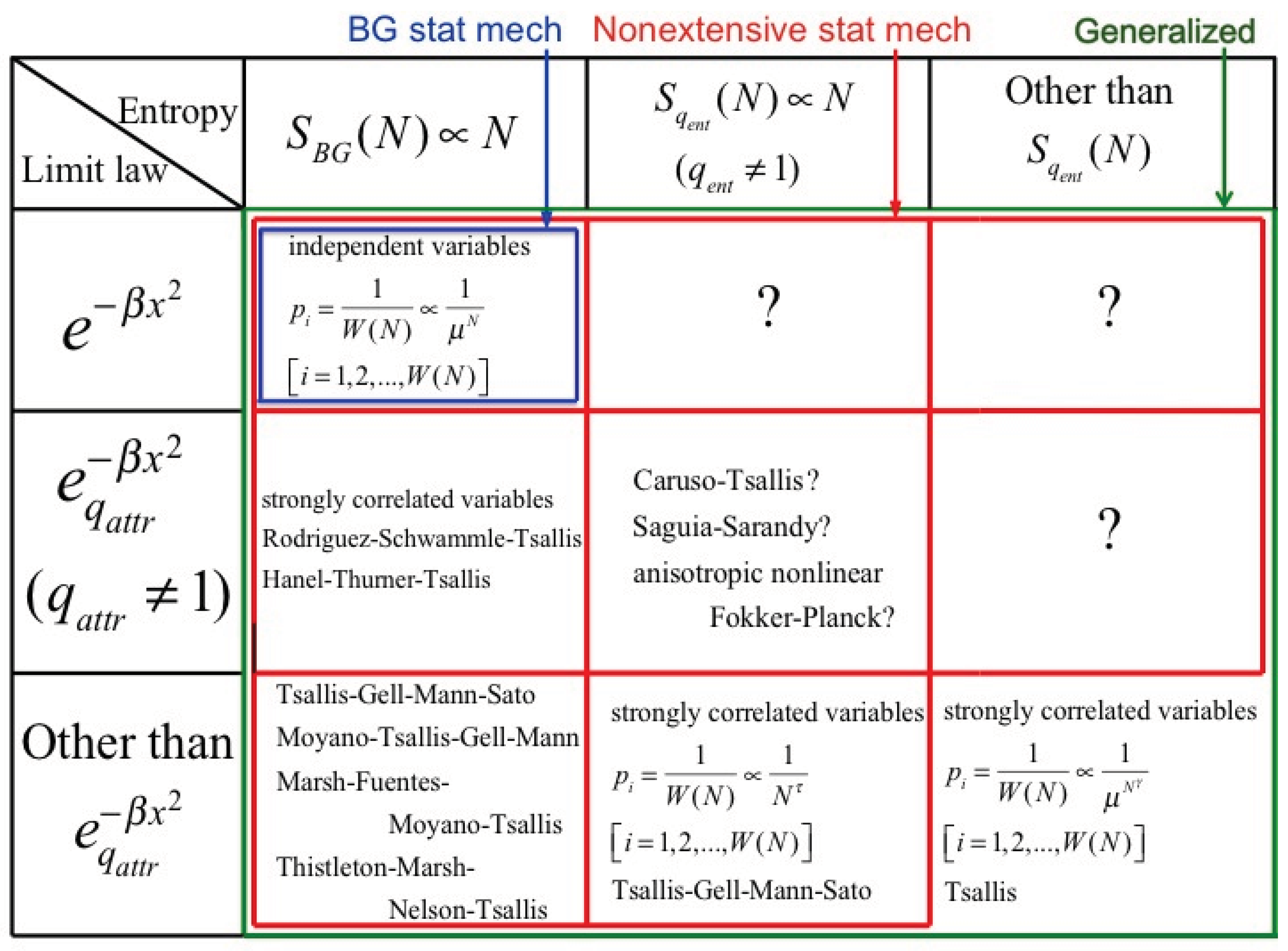
where by $W_{eff}\left(N\right)$ ($\le W\left(N\right)$) we denote the effective number of possible states, namely those whose probability is nonzero. We immediately verify that $S_{BG}\left(N\right)=kln{W}_{eff}\left(N\right)\propto lnN$, hence it is nonextensive for any system satisfying (16). In other words, it violates classical thermodynamics, and consequently we cannot use many of the formulas that are exhibited in all good textbooks of thermodynamics. It is to avoid such disagreeable situation that we are led to generalize the BG entropic functional.

Indeed, in remarkable contrast with $S_{BG}\left(N\right)$, $S_q\left(N\right)\propto N$ for

$$q=1-\frac{1}{\tau }$$

(17)

for all systems satisfying (16) [16] (another such example is shown in [17] with $\tau =d$, $d=1,2,3,...$, characterizing the width of the region of nonvanishing probabilities in an asymptotically scale-invariant probabilistic triangle of N identical and strongly correlated binary variables). For such complex systems, the additive entropy $S_{BG}$ is nonextensive, whereas the nonadditive entropy $S_q$ is extensive for a special (system-dependent) value of q, and therefore thermodynamically admissible! Various mathematical and physical examples are introduced and discussed in [16,17,18,19]. We shall hereafter note $q_{ent}$ the value of q such that $S_q\left(N\right)\propto N$. So, if the system satisfies Relation (15), we have $q_{ent}=1$, whereas if it satisfies Equation (16) we have $q_{ent}=1-\frac{1}{\tau }$ . It is convenient to emphasize at this point that particularly complex systems mathematically exist (and probably also exist in nature) for which no value q exists such that $S_q$ is extensive. We are therefore obliged, in such cases, to introduce other generalized entropic forms. Let us illustrate this fact with the following example [10]. If we have that

$$W_{eff}\left(N\right)\sim {\mu }^{N^{\gamma }}(N\to \infty ;\mu >1,0<\gamma <1)$$

(18)

we are led to consider the entropy

$$S_{\gamma }=k\sum _{i=1}^{W_{eff}}{p}_i{ln}^{1/\gamma }(1/p_i)(S_1=S_{BG})$$

(19)

whose equal-probability expression is given by

$$S_{\gamma }=k{ln}^{1/\gamma }{W}_{eff}$$

(20)

We immediately verify that $S_{\gamma }\left(N\right)\sim ({ln}^{1/\gamma }\mu )N$, hence extensive. It can be straightforwardly verified that $S_{\gamma }\left(\left\{p_i\right\}\right)$ is nonnegative, expansible, concave, and nonadditive. A full classification of such behaviors has been proposed in [20].

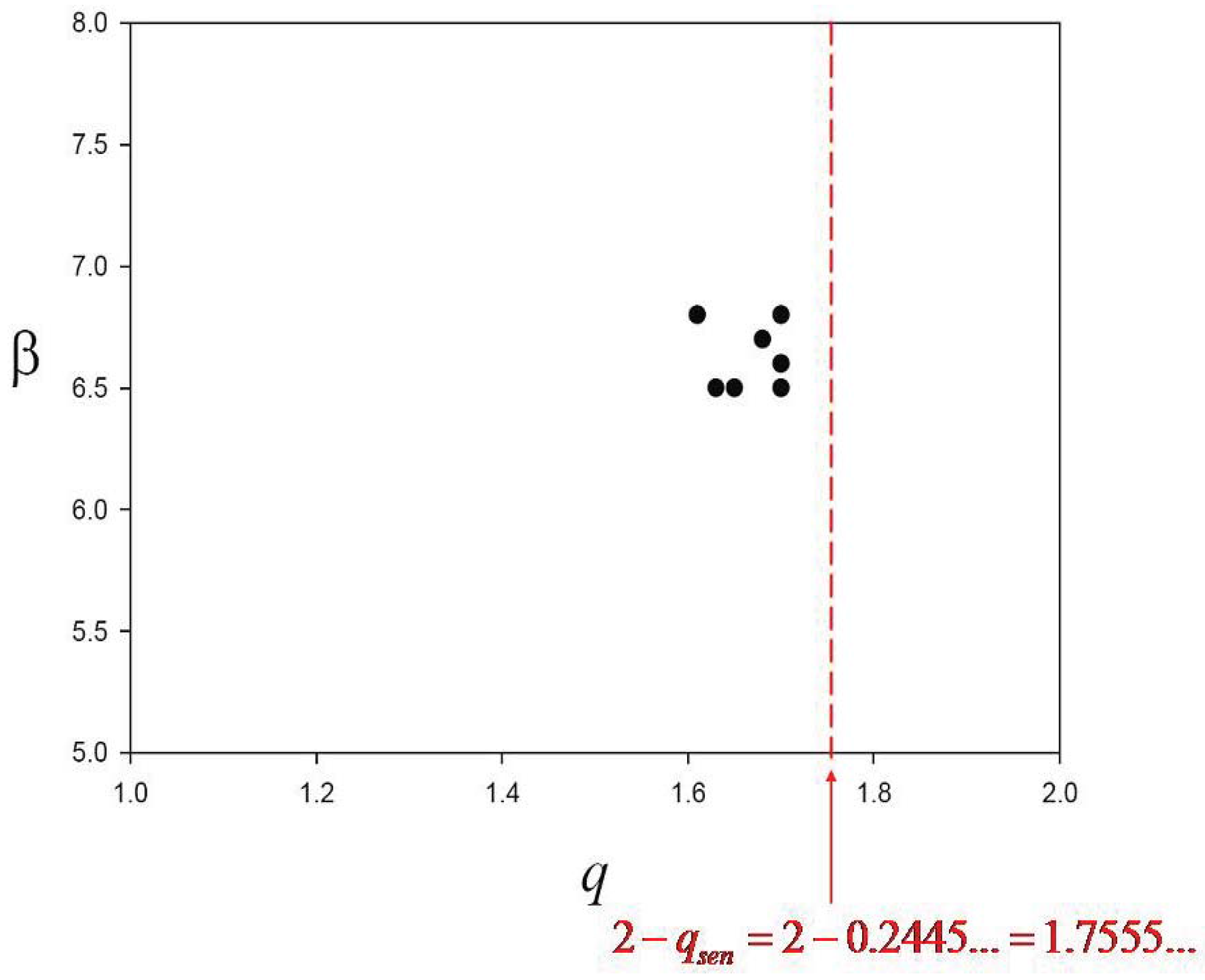
Let us now briefly review physical examples [18,19] having essentially this type of mathematical structure, and needing the use of $S_q$ with $q<1$ in order to satisfy classical thermodynamics for a subsystem of a quantum strongly entangled system. They both are finite-spin one-dimensional magnetic systems of N spins (a pure magnet in [18], and a random magnet in [19]). They both are considered at zero temperature, at the critical point of a quantum second-order phase transition. The state that is considered is the fundamental one in the $N>>1$ limit (i.e., the thermodynamic limit). The entropy of the N system is of course zero. But if we focus on a L-subsystem, namely a block of L consecutive spins in the interior of the N-system, we have that the so-called block entropy ${lim}_{N\to \infty }{S}_{BG}(L,N)$ is nonextensive. More precisely, the marginal density matrix associated with the L-system corresponds not to a pure but to a mixed state, and therefore its entropy is different from zero. It can be shown that ${lim}_{N\to \infty }{S}_{BG}(L,N)\sim lnL(L>>1)$, hence it violates the thermodynamical requirement of extensivity. It has been shown in both examples (analytically for the pure magnet, and numerically for the random magnet) that a special value of q, $q_{ent}<1$, exists such that ${lim}_{N\to \infty }{S}_{q_{ent}}(L,N)\sim L(L>>1)$, thus reconciling these strongly correlated systems with classical thermodynamics. The values of $q_{ent}$ as functions of the central charge c are shown in Figure 1. The scenario which emerges from these examples is the following one. Many quantum d-dimensional strongly-entangled systems exhibit, for their subsystems of size L, that

$$\begin{array}{ccc}\hfill S_{BG}\left(L\right)& \sim & lnL(d=1)\hfill \end{array}$$

(21)

$$\begin{array}{ccc}& \sim & L(d=2)\hfill \end{array}$$

(22)

$$\begin{array}{ccc}& \sim & L^2(d=3)\hfill \end{array}$$

(23)

$$\begin{array}{ccc}& \sim & L^{d-1}(d>1)\hfill \end{array}$$

(24)

The $d=3$ case corresponds to black holes, and the generic d-dimensional case is currently referred to in the literature as the area law. They can all be unified through

$$S_{BG}\left(L\right)\sim \frac{L^{d-1}-1}{d-1}\equiv {ln}_{2-d}L\ne L^d(d\ge 1)$$

(25)

and are nonextensive in all cases. The $d=1$ examples in [18,19] that we have discussed here above, as well as a bosonic $d=2$ one numerically approached in [18], suggest that a value of q $(q_{ent}<1)$ exists such that

$$S_{q_{ent}}\left(L\right)\sim L^d(d\ge 1)$$

(26)

i.e., extensive in all cases. It remains as an open intriguing puzzle what would be the value of $q_{ent}$ for black holes! Could it be $q_{ent}=1/2$? See $q_{ent}\left(c\right)$ for the pure magnet, in Figure 1. Indeed, on one hand, we obtain the value 1/2 for $c=4$ (it is known that, in some contexts, c behaves as a dimensionality, which is 4 for the relativistic space-time (the same viewpoint might perhaps explain why, in the limit $c\to \infty$, we obtain the BG value $q_{ent}=1$). On the other hand, the value 1/2 has already emerged in theoretical discussions of black holes [21].

To summarize the present Section we might emphasize that additivity only depends on the mathematical connection between the thermodynamic entropy and the nonvanishing probabilities of the admissible microscopic configurations [22]. Extensivity is more complex. Indeed, it not only depends on the above mathematical connection, but also on the class of correlations between the elements of the system. In other words, the validity of thermodynamics in what concerns the extensivity of the entropy mandates the admissible entropic forms. If the system satisfies Relation (15) we must use $S_{BG}$; if the system satisfies Relation (16) we must use $S_q$ with $q\ne 1$; if the system satisfies other relations, we must use other entropies. It is as simple as that! A sort of typical paradigm shift in the Thomas Kuhn sense [23] can be seen in this fact, where an universal (or so thought to be, more precisely speaking) expression for the entropy is to be replaced by a nonuniversal one which “dialogues” adequately with the class of correlations present in the system.

Let us finally clarify a misname that has been long used (and still is occasionally used) in the literature. The entropy $S_q$ has been frequently referred to as “nonextensive entropy” for $q\ne 1$. This is in general inadequate, and it should be referred to as “nonadditive entropy" instead. Indeed, once the adequate value of q is chosen, $S_q$ is thermodynamically extensive for all those systems for which it is applicable. Why then maintaining the expression “nonextensive statistical mechanics” to refer to the associated thermostatistical theory? Besides the historical fact that it is so called since more than two decades, there is the fact that it is intended to be applicable to long-range-interacting many-body Hamiltonian systems, which by definition have a nonextensive internal energy (see, for example, [24], as well as generic thermodynamical considerations reviewed in [10]), while the entropy remains extensive, as in the case of short-range interactions.

3. Probability Distributions that Are Attractors in the Sense of the Central Limit Theorem

In the $D=1$ continuous case, if an appropriate first moment of x is different from zero (see details in [6]), the extremization of $S_q$ yields

$$p\left(x\right)=\frac{e_q^{-\beta x}}{\int dx{e}_q^{-\beta x}}(q<2;\beta >0)$$

(27)

where $e_q^z$ is the inverse function of ${ln}_{q}z$, more precisely

$$e_q^z\equiv {[1+(1-q)z]}_{+}^{\frac{1}{1-q}}(e_1^z=e^z)$$

(28)

${[...]}_{+}$ being equal to its argument when this is positive, and zero otherwise [25]. Clearly Equation (27) recovers Equation (5) for the $q=1$ particular case. The condition $q<2$ comes from the demand of normalizability of Distribution (27) [26] (x is assumed to take values only for $x>x_{min}>-\infty$).

If the appropriate first moment vanishes and we happen to know the appropriate second moment, the extremization of $S_q$ yields, for the continuous case, the so-called q-Gaussian distribution

$$p\left(x\right)=\frac{e_q^{-\beta x^2}}{\int dx{e}_q^{-\beta x^2}}(q<3;\beta >0)$$

(29)

The q-Gaussian distributions [27] have a finite support for $q<1$, and an infinite one for $q\ge 1$; for $q>1$ they asymptotically decay as power-laws (more precisely like $x^{-2/(q-1)}$); they have a finite variance for $q<5/3$, and an infinite one for $q\ge 5/3$; they are normalizable only for $q<3$ [28].

Around 2000 [29], q-Gaussians have been conjectured (see details in [30]) to be attractors in the CLT sense whenever the N random variables that are being summed are strongly correlated in a specific manner. The conjecture was recently proved in the presence of q-independent variables [31,32,33,34,35]. The proof presented in [33] is based on a q-generalization of the Fourier transform, denoted as q-Fourier transform, and the theorem is currently referred to as the q-CLT. The validity of this proof has been recently challenged by Hilhorst [36,37]. His criticism is constructed on the inexistence of inverse q-Fourier transform for $q>1$, which he illustrates with counterexamples. The inverse, as used in the [33] paper, indeed does not exist in general, which essentially makes the proof in [33] a proof of existence, but not of uniqueness. The q-generalization of the inverse Fourier transform appears then to be a quite subtle mathematical problem if $q\ne 1$. It has nevertheless been solved recently [38,39], and further considerations are coming [40] related to q-moments [41,42,43]. Work is in progress attempting to transform the existence proof in [33] into a uniqueness one. It is fair to say that, at the present moment, a gap exists in the complete proof (not necessarily in the thesis) of the q-CLT as it stands in [33]. In the meanwhile, several other forms [44,45,46] of closely related q-generalized CLT’s have already been published which do not use the inverse q-Fourier transform.

Probabilistic models have been formulated [47,48] which, in the $N\to \infty$ limit, yield q-Gaussians. These models are scale-invariant, which might suggest that q-independence implies scale-invariance, but this is an open problem at the present time. However, definitively, scale-invariance does not imply q-independence. Indeed, (strictly or asymptotically) scale-invariant probabilistic models are known [49,50,51] which do not yield q-Gaussians, but other limiting distributions instead, some of which have been proved to be amazingly close to q-Gaussians [52]. In addition to all these, q-Gaussians are exact solutions of nonlinear homogeneous [53,54,55,56] as well as of linear inhomogeneous Fokker-Planck equations [57]. In fact, these various cases have been recently unified as particular cases of nonlinear inhomogeneous Fokker-Planck equations [58].

Let address now an interesting question, namely, whether it is possible to simultaneously have, in the same (mechanical or purely probabilistic) many-body system, an extensive entropy $S_{q_{ent}}$, and a $q_{attr}$-Gaussian distribution which is an attractor in the sense of the CLT (which, for mechanical systems, essentially corresponds to time averages, as opposed to ensemble averages).

It is clear that this situation trivially exists in the BG frame (for both probabilistic models, and thermostatistics of classical Hamiltonian systems), with $q_{ent}=q_{attr}=1$. The simplest probabilistic model is N independent binary random variables. The Gaussian attractor (i.e., $q_{attr}=1$) is since long known and basically constitutes the so-called de Moivre–Laplace theorem. Also, a straightforward calculation leads to $S_{BG}=k(ln2)N$ (i.e., $q_{ent}=1$). The simplest mechanical model is the ideal gas. The one-body distribution of velocities is the well known Maxwellian, hence $q_{attr}=1$, and, as proved in any statistical mechanics textbook, the associated BG entropy is extensive, hence $q_{ent}=1$.

The situation is of course nontrivial in the realm of nonextensive statistical mechanics, where at least one (and even possibly both) among $q_{ent}$ and $q_{attr}$ must differ from unity.

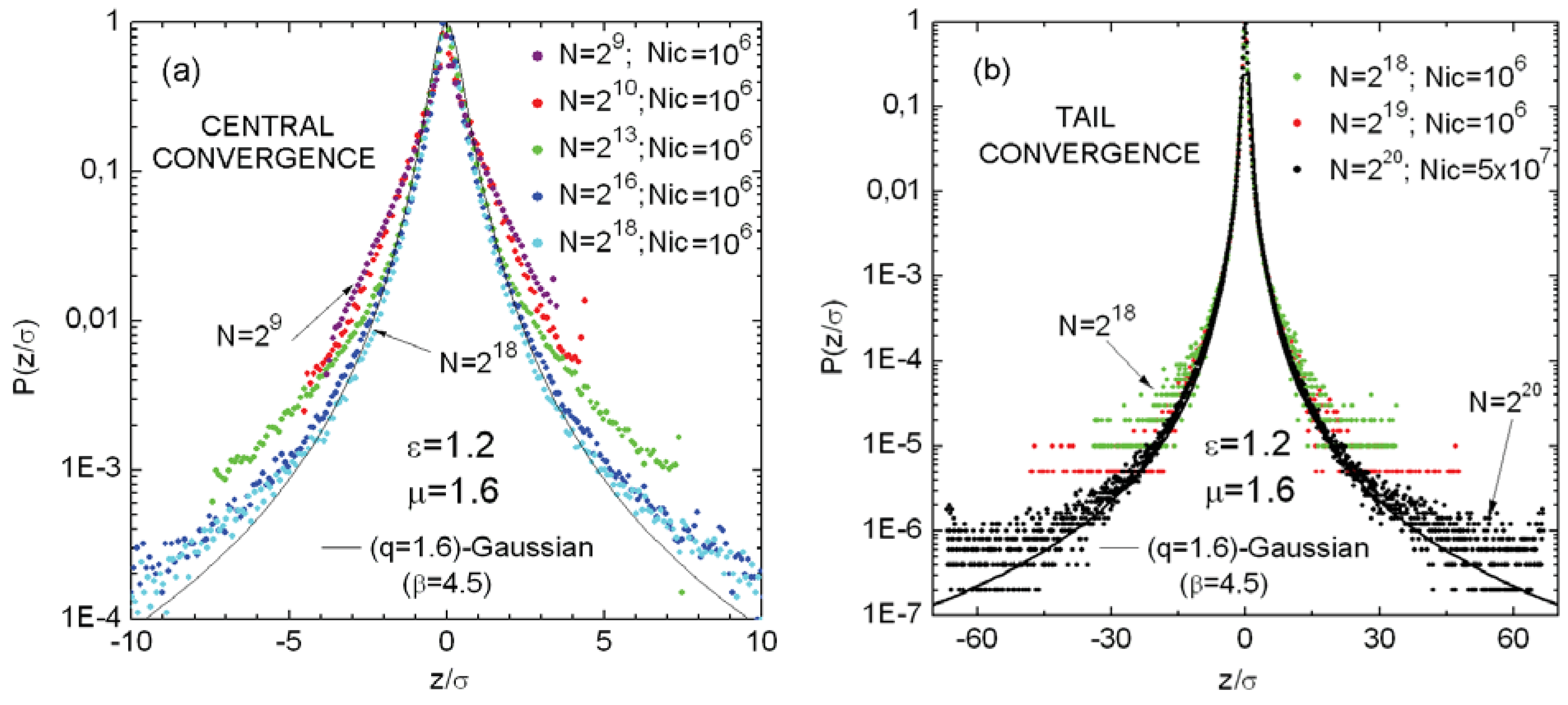
Let us first focus on probabilistic models. Simple models based on strongly correlated binary random variables exist for which the $N\to \infty$ limiting distributions are q-Gaussians with both $q_{attr}<1$ (compact support) [47,48] and $q_{attr}>1$ (heavy tails) [48]. To be precise, it has been proved that these are the limiting distributions, but it has not yet been specifically proved that they are attractors (i.e., stable distributions) in the space of probability distributions, although it might well be so. For all these models we have $q_{ent}=1$. What about those situations where $q_{ent}\ne 1$? We do not yet have clear-cut examples whose attractor is a $q_{attr}$-Gaussian, neither with $q_{attr}=1$ nor $q_{attr}\ne 1$. We do have, however, examples where the attractor is not a $q_{attr}$-Gaussian: see Figure 2.

A particularly interesting possibility would be that of simultaneously having $q_{ent}\ne 1$ and $q_{attr}\ne 1$. Such case is by no means trivial. Let us present here a mathematically possible and physically plausible manner through which this could happen.

Let us focus on a system such that $q_{attr}$ exist in the $N\to \infty$, and differs from unity. Inspection of Figure 2 shows that they tend to have $q_{ent}=1$. How to avoid, for such a system, that $q_{ent}$ approaches unity in the thermodynamic limit? If we could have, in some sense to be specified, an anisotropic system with N different “axes” or “directions”, each of them being associated to an index $q_{ent}^{\left(n\right)}\le 1$, we would expect for the total entropy to be associated to an index $q_{ent}$ satisfying [59]

$$\frac{1}{1-q_{ent}}=\sum _{n=1}^N\frac{1}{1-q_{ent}^{\left(n\right)}}$$

(30)

If the system is anomalous we expect of course to have $q_{ent}^{\left(n\right)}\ne 1$ ($\forall n$) (typically $q_{ent}^{\left(n\right)}<1$, $\forall n$), which would be consistent with the fact that we have already assumed that $q_{attr}\ne 1$. If the system is fully isotropic, all $q_{ent}^{\left(n\right)}$ should be equal and equal to $q_{ent}^{\left(1\right)}$. Then the heuristic relation in Equation (30) implies

$$\frac{1}{1-q_{ent}}=\frac{N}{1-q_{ent}^{\left(1\right)}}$$

(31)

hence,

$$1-q_{ent}\propto \frac{1}{N}$$

(32)

Plenty of examples exist in the literature (e.g., [60,61,62,63,64,65]) for which this relation is satisfied. All of them yield $q_{ent}=1$ in the thermodynamic limit. But, if the system is anisotropic, we may order $q_{ent}^{\left(n\right)}$ so that

$$\frac{1}{1-q_{ent}^{\left(1\right)}}\ge \frac{1}{1-q_{ent}^{\left(2\right)}}\equiv \frac{{\delta }_2}{1-q_{ent}^{\left(1\right)}}\ge ...\ge \frac{1}{1-q_{ent}^{\left(N\right)}}\equiv \frac{{\delta }_N}{1-q_{ent}^{\left(1\right)}}({\delta }_n\ge 0,\forall n)$$

(33)

Consequently, from Equation (30), we obtain

$$\frac{1}{1-q_{ent}}=\frac{1}{1-q_{ent}^{\left(1\right)}}\left(1+\sum _{n=2}^N{\delta }_n\right)$$

(34)

If $\Delta \equiv {lim}_{N\to \infty }\left(1+{\sum }_{n=2}^N{\delta }_n\right)\ge 1$ is finite, then

$$q_{ent}=1-\frac{1-q_{ent}^{\left(1\right)}}{\Delta }<1$$

(35)

It seems plausible that the results (with $q_{ent}<1$) that have been verified in [18,19] follow a path somehow analogous to the above one.

Before closing this section, let us briefly mention another aspect concerning q indices. Different physical properties correspond, in one way or another, to different moments, and ultimately to different q indices. The infinite number of q indices within each of such families are expected to be related among them, leaving space for a small number (possibly just one or two in simple cases) of independent values of q’s, which would determine the associated universality classes. The study of these classes and their internal relations still is in its infancy. However, some illustrations do exit, at least on the mathematical level. For example, the successive application of the additive duality $q\to (2-q)$ and the multiplicative duality $q\to 1/q$ determines the following algebras [17,33]:

$$\frac{2}{1-q_{m,2}^{+}}=\frac{2}{1-q_0}+m(m=0,\pm 1,\pm 2,...)$$

(36)

and

$$\frac{2}{1-q_{m,2}^{-}}=\frac{2}{q_0-1}+m(m=0,\pm 1,\pm 2,...)$$

(37)

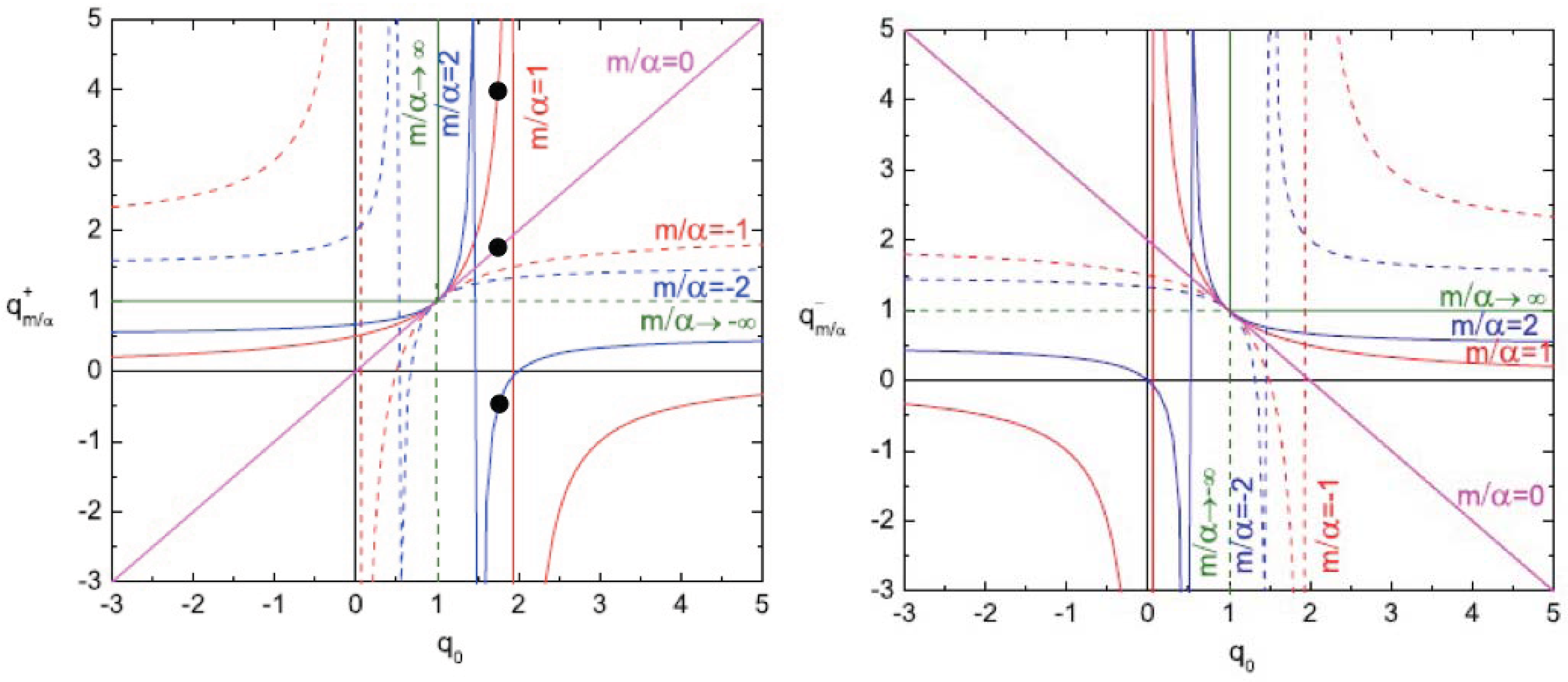
These algebras can be generalized into [34]

$$\frac{\alpha }{1-q_{m,\alpha }^{+}}=\frac{\alpha }{1-q_0}+m(m=0,\pm 1,\pm 2,...)$$

(38)

and

$$\frac{\alpha }{1-q_{m,\alpha }^{-}}=\frac{\alpha }{q_0-1}+m(m=0,\pm 1,\pm 2,...)$$

(39)

where $0<\alpha \le 2$. We immediately realize that $q_{m,\alpha }^{\pm }$ only depend on $(q_0,m/\alpha )$. In other words, the universality class is in this case determined by only two real numbers, namely $q_0$ and α. We also verify that if $q_0=1$, all of them are equal to unity, but, if $q_0\ne 1$, an infinite family of inter-related indices q appears (thus reflecting the relative simplicity of the BG statistical mechanics, as compared to the nonextensive one). These algebras are depicted in Figure 3 [66]. The q-triplets that have been frequently observed in nature (or in computational models) probably correspond to central elements of algebras like the one that we have just illustrated, or of similar mathematical structures.

4. Remarks on Paradigmatic Low-Dimensional Nonlinear Dynamical Systems Near the Edge of Chaos

As we have seen in Section 2 of this review, the strong utility of the BG entropy relies on the fact that the N random variables of the system might be independent or nearly so. If this hypothesis is not satisfied, then we should have recourse to other entropies, for instance $S_q$. Now, what is the situation for a nonlinear dynamical system? Strong chaos, i.e., positive largest Lyapunov exponent (LLE) in systems whose random variables are continuous, makes the correlation between not too close elements of the system, and even successive steps of the same element, to be quickly lost. Therefore in such dynamical systems, the hypothesis of probabilistic independence is essentially satisfied. This is what Boltzmann intuitively referred to as the Stossanzahlansatz (molecular chaos hypothesis). What happens then when the LLE approaches zero, or even vanishes? We should observe the failure (or, at least, inadequacy) of the BG entropic form and of its consequences (very especially, the ubiquity of exponential and Gaussian laws).

Let us illustrate these features in simple low-dimensional dynamical systems, namely one-dimensional dissipative unimodal maps, and two-dimensional conservative maps.

4.1. One-Dimensional Dissipative Unimodal Maps

Let us focus on the z-logistic map, defined as follows

$$x_{t+1}=1-a{\left|x_t\right|}^z(0\le a\le 2;z\ge 1;x_t\in [-1,1];t=0,1,2,3,...)$$

(40)

These maps exhibit, for $a<a_c\left(z\right)$ (where $a_c\left(z\right)$ monotonically increases from 1 to 2 when z increases from 1 to infinity), attractors which are fixed points, cycles-2, cycles-4, and so on. While a approaches the value $a_c\left(z\right)$ from below, these attractors successively bifurcate, and the bifurcation points accumulate at $a_c\left(z\right)$, the edge of chaos, sometimes referred to as the Feigenbaum point. For $a>a_c\left(z\right)$, a complex behavior emerges, with many peculiarities. Among those, a remarkable one is the fact that infinitely many intervals of a exist for which the (unique) Lyapunov exponent ${\lambda }_1$ is positive (the subindex 1 will soon become clear), whereas no such possibility exists for $a<a_c\left(z\right)$. The largest value of ${\lambda }_1$ occurs at $a=2,\forall z$; at the edge of chaos, ${\lambda }_1$ vanishes. For every value of a whose ${\lambda }_1$ is positive, we observe the following properties.

(i) The sensitivity to the initial conditions $\xi \left(t\right)\equiv {lim}_{\Delta \left(0\right)\to 0}\frac{\Delta \left(t\right)}{\Delta \left(0\right)}$ diverges exponentially, namely

$$\xi \left(t\right)=e^{{\lambda }_{1}t}$$

(41)

(ii) If we start at $t=0$ with a uniform occupancy of initial conditions in the interval $[-1,1]$, the generic case is that the occupancy region gradually shrinks with t. The number $W\left(t\right)$ of little windows which contain at least one point decays exponentially, essentially as follows:

$$\frac{W\left(t\right)-W\left(\infty \right)}{W\left(0\right)-W\left(\infty \right)}=e^{-t/{\tau }_1}(W\left(\infty \right)>0)$$

(42)

(iii) If we make a partition of the interval $[-1,1]$ in many W equal little windows ($i=1,2,...,W$), and fill, at $t=0$, one of them (say near the origin) with many M initial conditions (for instance, randomly spread within that little initial window), we can define a set of probabilities $p_i\left(t\right)\equiv \frac{M_i\left(t\right)}{M}$, where $M_i\left(t\right)$ is the number of points present in the $i^{th}$-interval at time t (with ${\sum }_{i=1}^W{M}_i\left(t\right)=M$). With this set of probabilities we verify the following Pesin-like equality

$$\begin{array}{ccc}\hfill K_{BG}\equiv K_1& \equiv & \underset{t\to \infty }{lim}\underset{W\to \infty }{lim}\underset{M\to \infty }{lim}\frac{S_{BG}\left(t\right)}{t}\hfill \\ & =& \underset{t\to \infty }{lim}\underset{W\to \infty }{lim}\underset{M\to \infty }{lim}\frac{-{\sum }_{i=1}^W{p}_i\left(t\right)ln{p}_i\left(t\right)}{t}={\lambda }_1\hfill \end{array}$$

(43)

The entropy production per unit time $K_{BG}$ here defined is a concept similar to the so-called Kolmogorov–Sinai entropy rate, and is expected to provide the same result in most cases.

(iv) If we make the sum of very many (plausibly infinitely many) successive values of $x\left(t\right)$ starting from a given generic initial condition we obtain, after appropriate centering and scaling, a Gaussian distribution

$$p\left(x\right)=\frac{e^{-\beta x^2}}{{\int }_{-\infty }^{\infty }dx{e}^{-\beta x^2}}$$

(44)

where β depends on $(a,z)$ and decreases for decreasing ${\lambda }_1$. This corresponds to the standard Central Limit Theorem (CLT), and reflects the (experimentally most important) time averages (as opposed to ensemble averages, i.e., averages over initial conditions).

(v) If we distribute within the interval $[-1,1]$ traps such that a point which falls there disappears from the system, the number of trajectories $N\left(t\right)$ that remain in the system from the initial $N\left(0\right)$ ones decreases exponentially as follows

$$\underset{N\left(0\right)\to \infty }{lim}\frac{N\left(t\right)}{N\left(0\right)}=e^{-{\gamma }_{1}t}$$

(45)

where the escape rate ${\gamma }_1$ depends on $(a,z)$ and decreases for decreasing ${\lambda }_1$. The relation (43) becomes generalized into

$$K_1={\lambda }_1-{\gamma }_1$$

(46)

Let us now address a highly interesting question, namely what happens at the edge of chaos, where ${\lambda }_1=0$ ? The answer is astonishingly simple. Essentially it suffices to replace (with some adjustments), in Equations (41)–(46), the subindex “BG", i.e., “1”, by the appropriate “q” indices! Let us review one by one the five above properties.

(i) The sensitivity to the initial conditions follows a behavior which asymptotically (i.e., for $t>>1$) is a power-law [68] (see also previous references in [10]). Details are analyzed in [68,69,70,71,72,73] and in references therein.

The (maximal) sensitivity ξ is given by

$$\xi =e_{q_{sen}}^{{\lambda }_{q_{sen}}t}$$

(47)

where [74] (see also [75])

$$\frac{1}{1-q_{sen}}={\lambda }_{q_{sen}}=\frac{1}{{\alpha }_{min}}-\frac{1}{{\alpha }_{max}}(q_{sen}<1)$$

(48)

where ${\alpha }_{min}$ and ${\alpha }_{max}$ are respectively the minimal and maximal values of the index α in the multifractal $f\left(\alpha \right)$ function [76]. This expression can be shown to be, for the z-logistic map,

$$\frac{1}{1-q_{sen}\left(z\right)}=(z-1)\frac{ln{\alpha }_F\left(z\right)}{ln2}$$

(49)

where ${\alpha }_F\left(z\right)$ is the Feigenbaum constant. For $z=2$ we have

$$q_{sen}\left(2\right)=0.244487701341282066198....$$

(50)

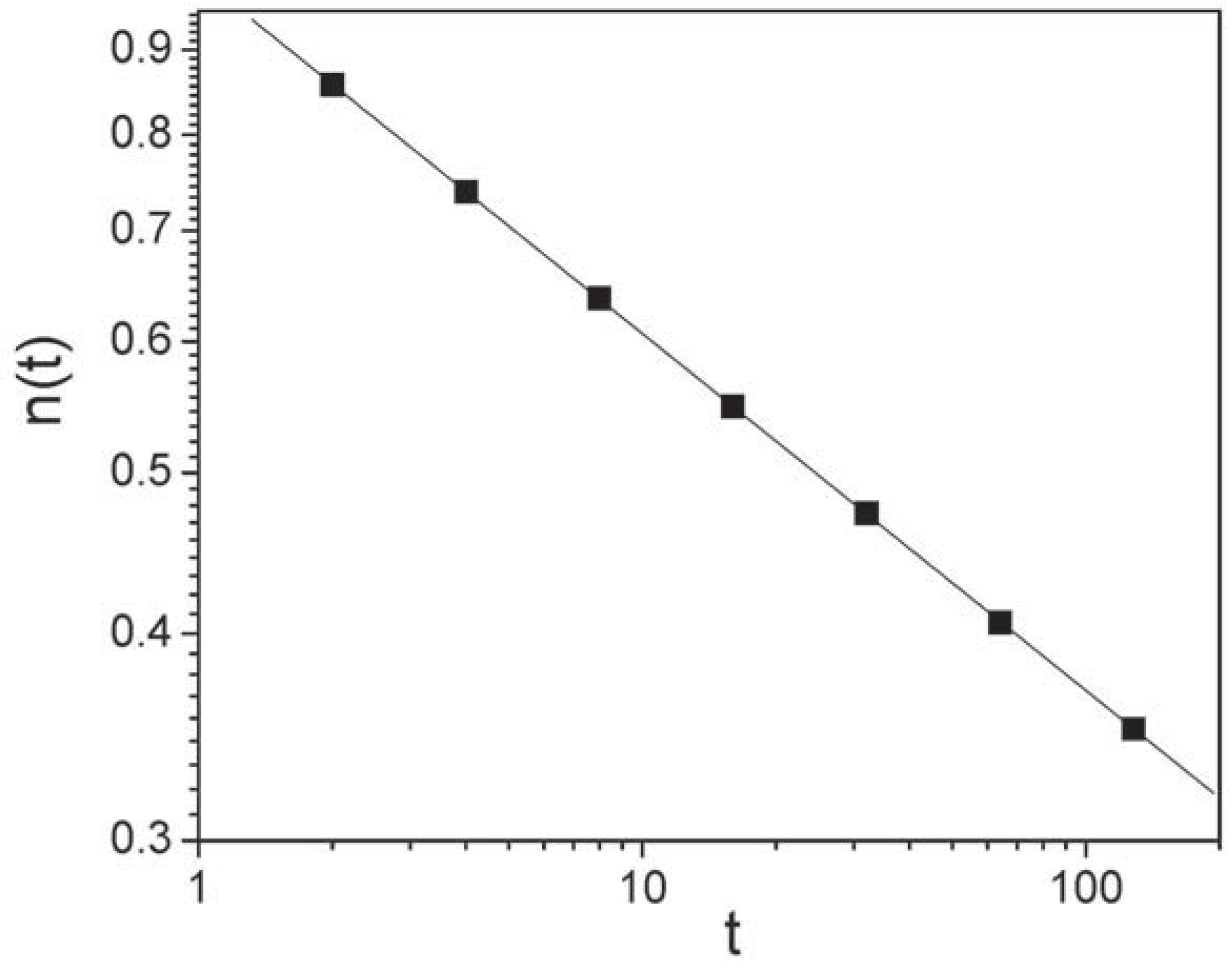
(ii) The Lebesgue measure of the intervals which contain at least one point decays approximatively like

$$\frac{W\left(t\right)}{W\left(0\right)}=e_{q_{rel}}^{-t/{\tau }_{q_{rel}}}(W\left(\infty \right)=0)$$

(51)

($rel$ stands for relaxation) with $q_{rel}\left(z\right)>1$ (see details in [10] and references therein). High precision calculations are available for $z=2$ [77,78] (see note [79]), namely $1/[q_{rel}\left(2\right)-1]=0.800138194...$, hence

$$q_{rel}\left(2\right)=2.249784109...$$

(52)

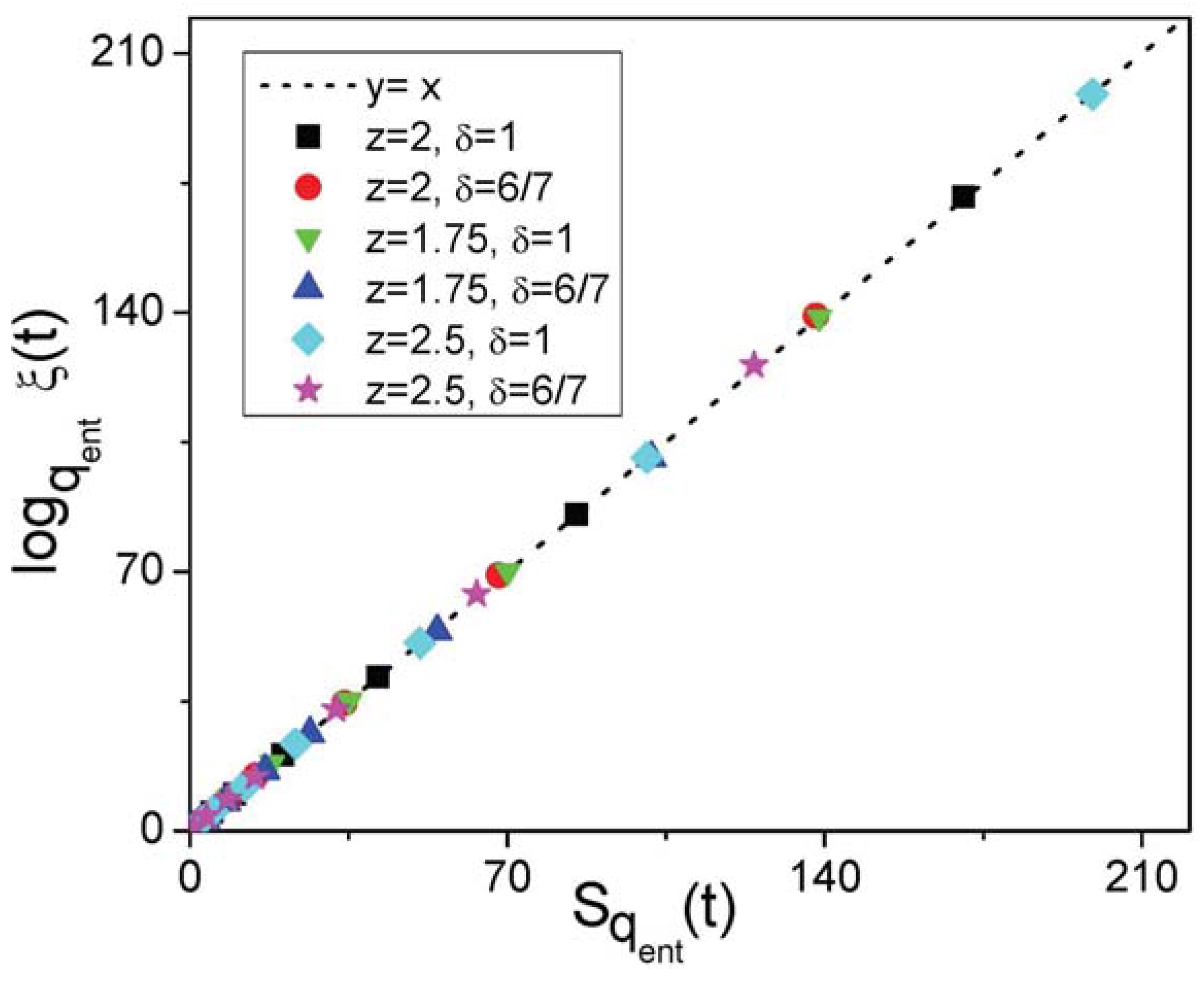
(iii) The (upper bound of the) entropy production per unit time is generalized as follows:

$$\begin{array}{ccc}\hfill K_{q_{sen}}& \equiv & \underset{t\to \infty }{lim}\underset{W\to \infty }{lim}\underset{M\to \infty }{lim}\frac{S_{q_{sen}}\left(t\right)}{t}\hfill \\ & =& \underset{t\to \infty }{lim}\underset{W\to \infty }{lim}\underset{M\to \infty }{lim}\frac{1-{\sum }_{i=1}^W{\left[p_i\left(t\right)\right]}^{q_{sen}}}{(q_{sen}-1)t}={\lambda }_{q_{sen}}\hfill \end{array}$$

(53)

(iv) The sum of very many successive values of $x\left(t\right)$ starting from a given generic initial condition yields (see details in [80,81,82]) (see note [83]), after appropriate centering and scaling, a $q_{timeave}$-Gaussian distribution (time ave stands for time average)

$$p\left(x\right)=\frac{e_{q_{timeave}}^{-{\beta }_{q_{timeave}}{x}^2}}{{\int }_{-\infty }^{\infty }dx{e}_{q_{timeave}}^{-{\beta }_{q_{timeave}}{x}^2}}$$

(54)

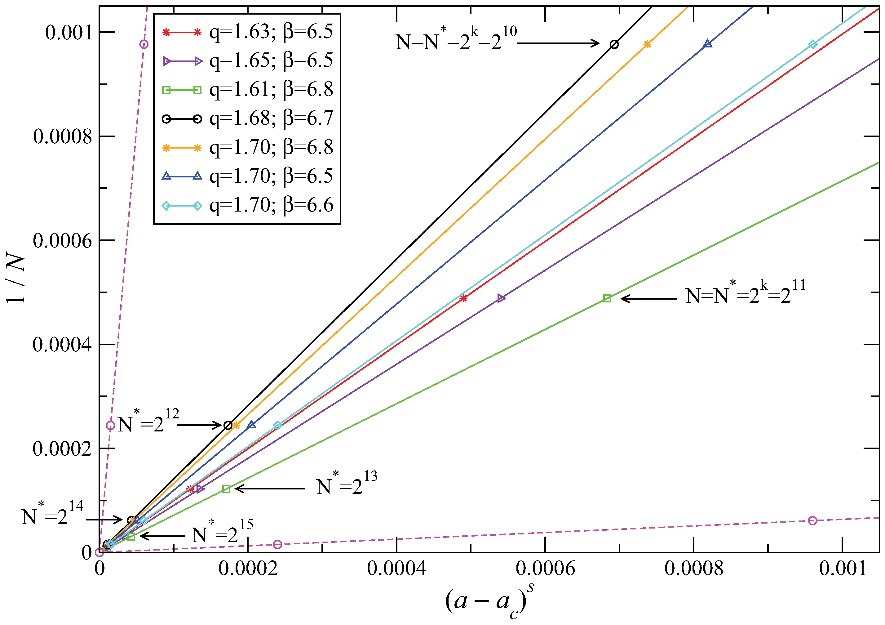
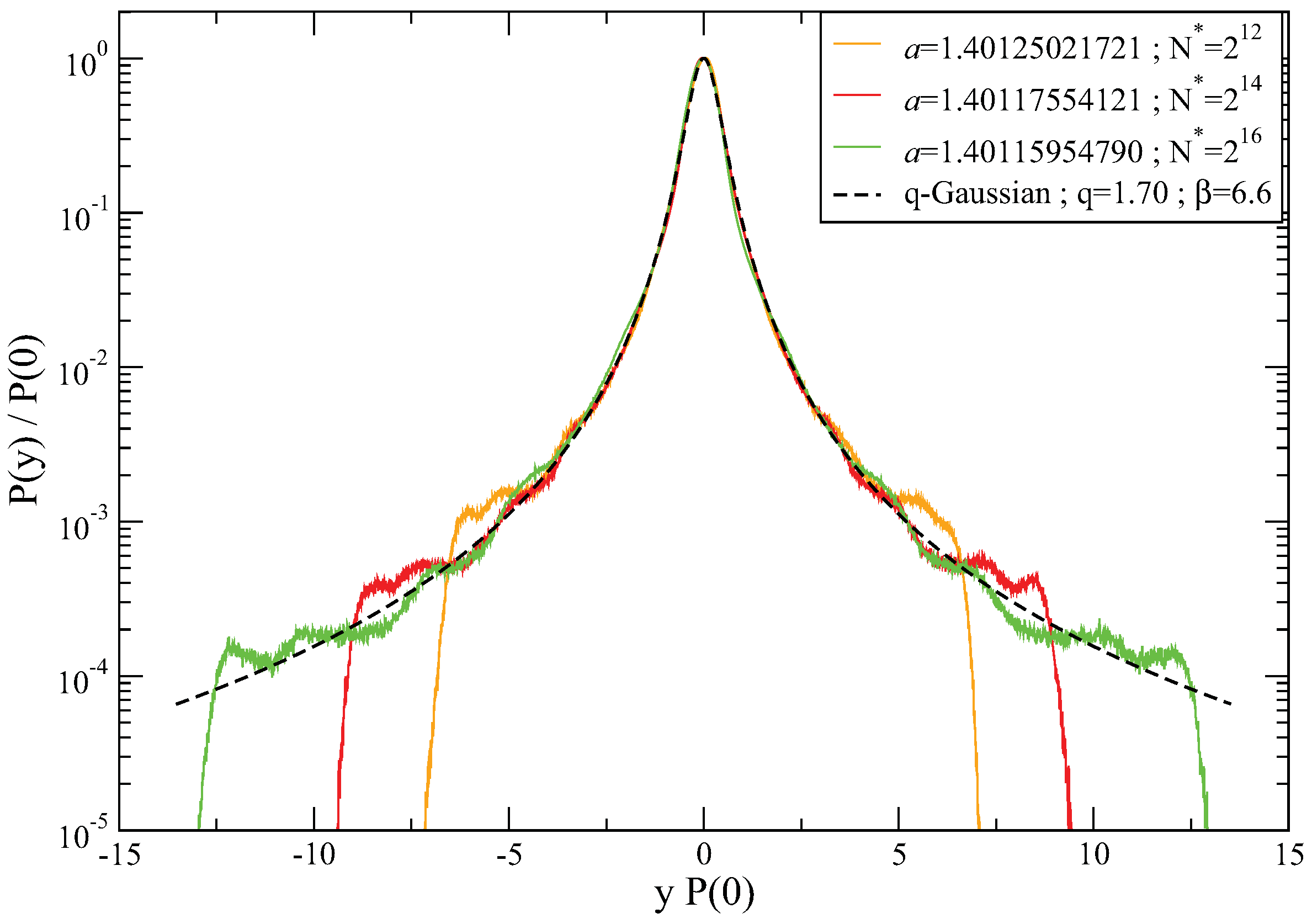
where $q_{timeave}\left(z\right)$ and ${\beta }_{q_{timeave}}\left(z\right)$ depend on z. This is not surprising given the q-Central Limit Theorem (CLT). However, an important difference exists with the $q=1$ generic case. It is here necessary to basically scale the number N of successive iterations with the “distance” (from above) to the edge of chaos $a_c\left(z\right)$ at which the calculation is being done [80,81,82]: see Figure 4, Figure 5 and Figure 6. In other words, it has a nature close to a crossover in the language of the usual critical phenomena theory. This point has been further analyzed in [84,85]. The present results suggest

$$q_{timeave}\left(2\right)=1.65\pm 0.05$$

(55)

(v) For the escape problem due to traps distributed within the interval $[-1,1]$, we obtain [86]

$$\underset{N\left(0\right)\to \infty }{lim}\frac{N\left(t\right)}{N\left(0\right)}=e_{q_{esc}}^{-{\gamma }_{q_{esc}}t}$$

(56)

where the escape rate ${\gamma }_{q_{}}\left(z\right)$ depends on z. The Relation (53) becomes generalized into

$$K_{q_{entprod}}={\lambda }_{q_{sen}}-{\gamma }_{q_{esc}}$$

(57)

where $entprod$ stands for entropy production per unit time. See typical illustrations in Figure 7 and Figure 8.

The values indicated in Equations (50), (52) and (55) play the role of the q-triplet for the $z=2$ logistic map.

Many of the results that have been here exhibited for the z-logistic map are also available in the literature for other families of maps (see, for instance, [87,88]). In all these various examples we verify that $q_{sen}\le 1$ (even $q_{sen}\le 0$ in some cases), and $q_{rel}\ge 1$; $q_{attr}$ can be either unity, above unity and below unity. The full mathematical clarification of these various possibilities remains elusive at the present time.

4.2. Two-Dimensional Conservative Maps

The type of results that have just been reviewed have been also seen in low-dimensional conservative maps in cases where the Lyapunov exponents (strictly or nearly) vanish. Such is the case in the Casati–Prosen triangle map [89] (where $q_{sen}=q_{entprod}=0$, and $K_{q_{entprod}}={\lambda }_{q_{sen}}=1$ have been verified), as well as in the MacMillan map [90] (where $q_{attr}\simeq 1.6$ has been numerically exhibited).

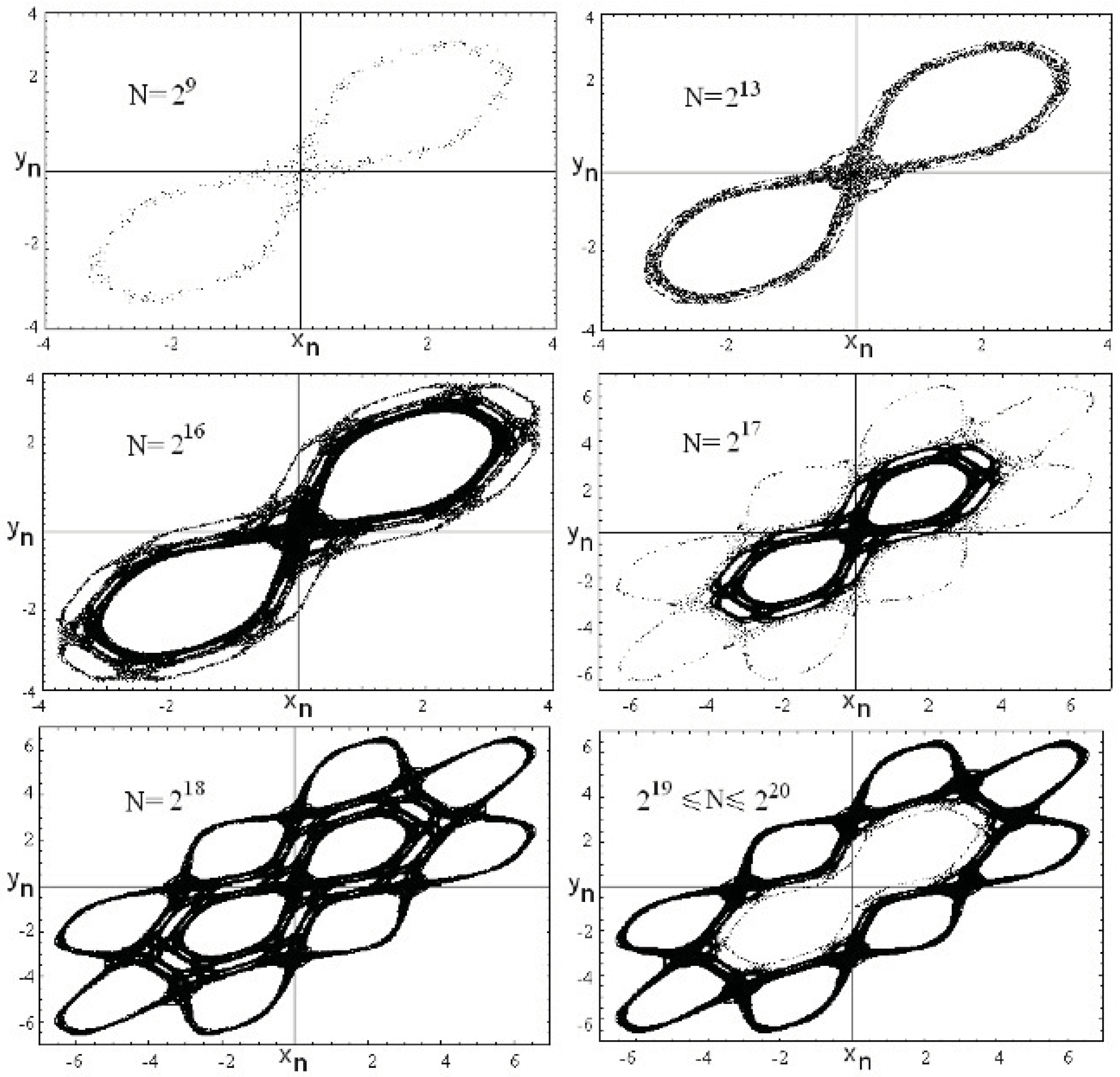
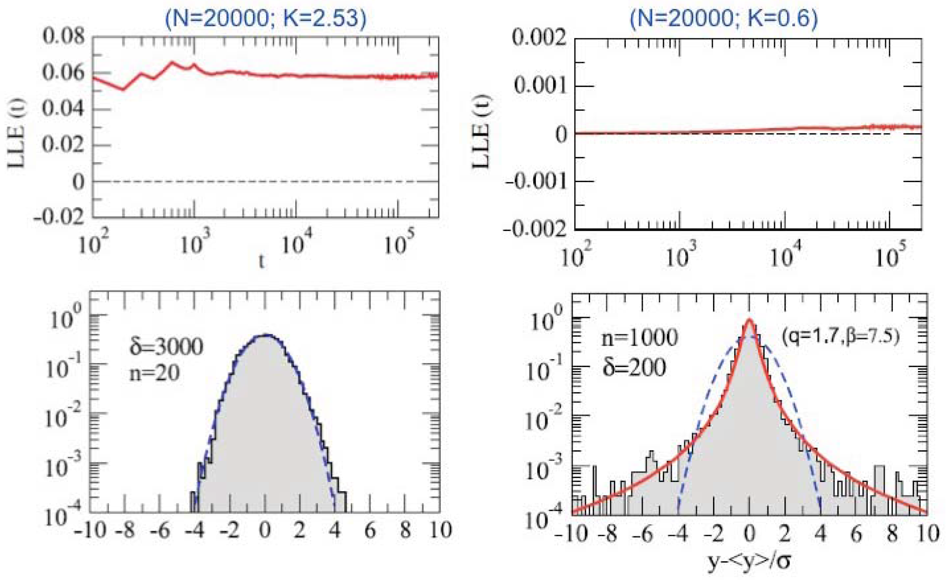
Specifically, the MacMillan map (physically relevant for focusing of thin lenses) is defined as follows:

$$\begin{array}{ccc}\hfill x_{t+1}& =& y_t\hfill \\ \hfill y_{t+1}& =& -x_t+2\mu \frac{y_t}{1+y_t^2}+ϵy_t\hfill \end{array}$$

(58)

which, for $\mu \ne 0$, is nonlinear. For $(\mu ,ϵ)=(1.6,1.2)$, the positive Lyapunov exponent equals a low value, namely 0.05, for orbits starting near the origin. See Figure 9 and Figure 10 in order to verify that, even for very large values of the number of iterations N, no sign towards ergodicity emerges. Instead the occupation of the phase-space remains sort of hierarchical. The distribution of sums (of successive values of the variable x) indeed suggests, after appropriate centering and scaling, a $q_{attr}$-Gaussian with $q_{attr}>1$. We do not know what is the situation in the mathematical $N\to \infty$ limit. But it is clear that a long-standing heavy-tailed distribution emerges in this problem.

5. Remarks on Paradigmatic Long-Range-Interacting Many-Body Classical Hamiltonian Systems

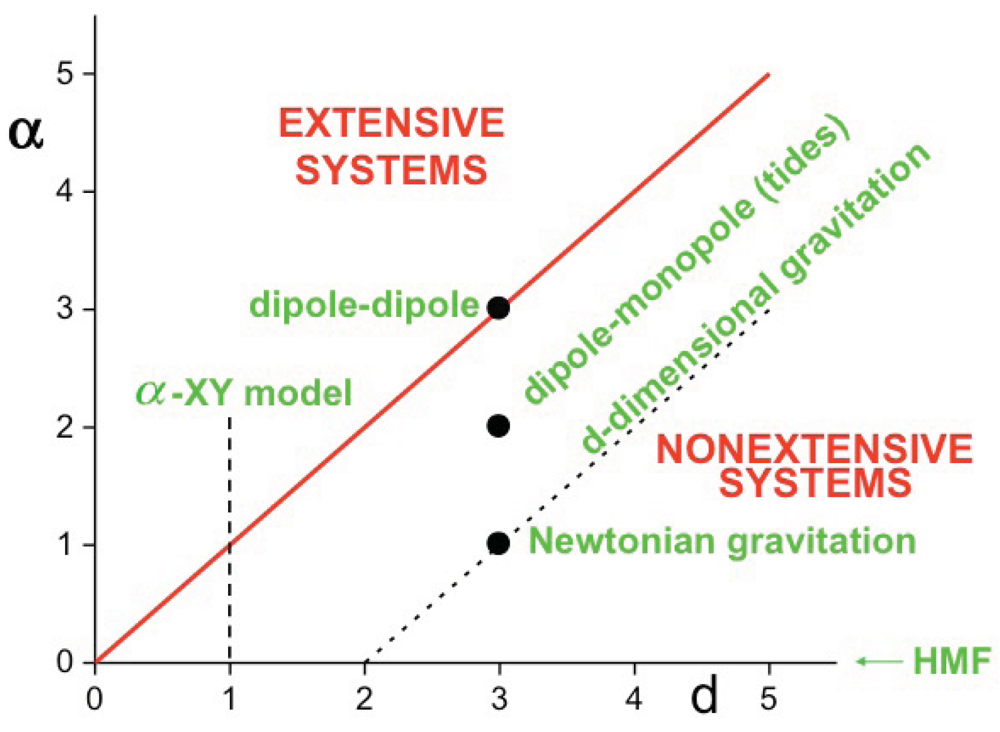
Let us focus now on a very interesting problem, namely that of classical d-dimensional many-body Hamiltonians involving N elements interacting through two-body potentials $V\left(r\right)$ that exhibit no singularities at short distances, are finite at intermediate distances, and have an attractive isotropic potential at long distances decaying like $r^{-\alpha }$ ($\alpha \ge 0$). A necessary condition for the existence of a finite BG partition function at all temperatures is that the potential be integrable. In other words, it is necessary that ${\int }_0^{\infty }dr{r}^{d-1}V\left(r\right)<\infty$, which implies that ${\int }_{r_0}^{\infty }dr{r}^{d-1}{r}^{-\alpha }<\infty$, $r_0$ being any finite distance. It can then be straightforwardly verified that this integrability is equivalent to the condition $\alpha /d>1$. In other words, if this condition is satisfied, the interaction will be referred to as short-ranged, and the BG statistical mechanical mathematical recipes are computable, finite results are obtained in virtually all circumstances (an exception is the second-order critical points in phase transitions), and the total internal energy is extensive (i.e., it grows like N). If $0\le \alpha /d<1$, the system potential is not integrable, the interaction will be referred to as long-ranged, no legitimate BG computations are tractable (unless we artificially scale the microscopic coupling constants with N: see [24]), and the total internal energy is super-extensive (i.e., it grows faster than N). These cases are summarized in Figure 11. The total energy of the N-system typically satisfies the following scaling (see [10] and references therein):

$$\begin{array}{c}\hfill U\left(N\right)\propto N\frac{N^{1-\alpha /d}-1}{1-\alpha /d}\end{array}$$

(59)

i.e.,

$$\begin{array}{ccc}\hfill U\left(N\right)& \propto & N(if\alpha /d>1)\hfill \end{array}$$

(60)

$$\begin{array}{ccc}& \propto & NlnN(if\alpha /d=1)\hfill \end{array}$$

(61)

$$\begin{array}{ccc}& \propto & N^{2-\alpha /d}(if0\le \alpha /d<1)\hfill \end{array}$$

(62)

Integrability of the potential is necessary for legitimate BG thermostatistics to be computable [91], and is consistent with the fact that, in the $N\to \infty$ limit, the largest Lyapunov exponent remains positive, whereas it approaches zero when the potential is non integrable (see examples in [24,92,93]). However, BG computability does not in principle guarantee that the main stationary (or quasi-stationary) state is precisely the BG thermal equilibrium: ergodicity is required as well, which might be not the case for finite N (perhaps not even in the $N\to \infty$ limit). An illustration of this fact is provided by the α-XY ferromagnet [24]. A preliminary discussion has been recently presented [94] for the $d=1$ model. Robust q-Gaussians are observed for a wide variety of conditions. One such example is shown in Figure 12 for $\alpha =0.99$ and $N=300000$.

Also for confining potentials (e.g., for $V\left(r\right)\propto r^{-\alpha }$ with $\alpha <0$), interesting similar situations can be observed. Such is the case for the Fermi–Pasta–Ulam β model for finite N, as recently shown [95,96]: Gaussian distributions of momenta are observed for time averages far from its π-orbit (consistently with the CLT), whereas (strict or approximate) q-Gaussians emerge very close to it. See Figure 13.

Let us mention that similar features can also occur in dissipative many-body systems. Such is the case in the Kuramoto model of N nonlinearly coupled oscillators, as illustrated in Figure 14 [97].

The distributions observed in Figure 12, Figure 13 and Figure 14 have been satisfactorily fitted with q-Gaussians. It is nevertheless clear that although this fact constitutes a strong suggestion, it does not prove that they are indeed q-Gaussians, no more than the thousands of fittings done during the last one hundred years with Gaussians for all kinds of physical systems do not prove that they indeed are Gaussians. In particular, we must always have in mind that distributions such as the Lévy (see, for instance, [98,99]) and the $(q,\alpha )$-stable (see [34]) ones exhibit, like many others, similar forms.

6. Applications

In this Section we briefly, and non-exhaustively, review various predictions, verifications and applications of q-exponentials and q-Gaussians through analytical, experimental, observational and computational methods in natural, artificial and social systems that are available in the literature (see [100] for full bibliography).

(i)

The velocity distribution of (cells of) Hydra viridissima follows a q-Gaussian probability distribution function (PDF) with $q\simeq 3/2$ [101,102]. Anomalous diffusion has been independently measured as well [101,102], and an exponent $\gamma \simeq 4/3$ has been observed (where the squared space $x^2$ scales with time t like $t^{\gamma }$). Therefore, within the error bars, the prediction $\gamma =\frac{2}{3-q}$ [54] is verified in this system.

(ii)

The velocity distribution of (cells of) Dictyostelium discoideum is well fitted by a q-Gaussian PDF with $q\simeq 5/3$ in the vegetative state, and with $q\simeq 2$ in the starved state [103].

(iii)

The velocity distribution of the point defects in in defect turbulence, as well as its corresponding anomalous diffusion, have been measured [104]. The results suggest a q-Gaussian PDF with $q\simeq 3/2$, and $\gamma \simeq 4/3$, which constitutes another verification of the prediction $\gamma =\frac{2}{3-q}$ [54].

(iv)

The velocity distribution of cold atoms in a dissipative optical lattice was predicted [105] to be a q-Gaussian with $q=1+44\frac{E_r}{U_0}$, where $E_r$ and $U_0$ are parameters related to the optical lattice potential. This prediction was verified three years later, both in the laboratory and with quantum Monte Carlo techniques [106,107].

(v)

Computational simulations of the velocity distribution, and of the associated anomalous diffusion, during silo drainage suggest $q\simeq 3/2$ and $\gamma \simeq 4/3$ [108,109], once again satisfying the prediction $\gamma =\frac{2}{3-q}$ [54].

(vi)

The velocity distribution in a driven-dissipative 2D dusty plasma was found to be of the q-Gaussian form, with $q=1.08\pm 0.01$ and $q=1.05\pm 0.01$ at temperatures of $30000K$ and $61000K$ respectively [110].

(vii)

The spatial (Monte Carlo) distributions of a trapped ${}^{136}B{a}^{+}$ ion cooled by various classical buffer gases at $300K$ was verified to be of the q-Gaussian form, with q increasing from close to unity to about 1.9 when the mass of the molecules of the buffer increases from that of $He$ to about 200 [111].

(viii)

The distributions of price returns and stock volumes at the New York and NASDAQ stock exchanges are well fitted by q-Gaussians and q-exponentials respectively [112,113,114,115]. The volatility smiles that are obtained within this approach also are well fitted. The distributions of interoccurrence times between losses in financial markets are consistently well described by universal q-exponentials, which enables a simple analytical expression for the risk function [116].

(ix)

The Bak–Sneppen model of biological evolution exhibits a time-dependence of the spread of damage which is well approached by a q-exponential with $q<1$ [117].

(x)

The distributions of returns in the Ehrenfest’s dog-flea model exhibit a q-Gaussian form [118,119].

(xi)

The distributions of returns in the coherent noise model are well fitted with q-Gaussians where q is analytically obtained through $q=\frac{2+\tau }{\tau }$, τ being the exponent associated with the distribution of sizes of the events [120].

(xii)

The distributions of returns of the avalanche sizes in the self-organized critical Olami–Feder–Christensen model, as well as in real earthquakes exhibit a q-Gaussian form [121] (see also [122]).

(xiii)

The distributions of angles in the $HMF$ model approaches as time evolves towards a q-Gaussian form with $q\simeq 1.5$ [123].

(xiv)

Experimental measurements of the turbulence in pure electron plasma are analytically reproduced with $q=1/2$ [124,125].

(xv)

The relaxation in various paradigmatic spin-glass substances through neutron spin echo experiments is well reproduced by q-exponential forms with $q>1$ [126].

(xvi)

The fluctuating time dependence of the width of the ozone layer over Buenos Aires (and, presumably, around the Earth) yields a q-triplet with $q_{sen}<1<q_{statstate}<q_{rel}$ [127].

(xvii)

Diverse properties for conservative and dissipative nonlinear dynamical systems (different from those described earlier in this review) are well described within q-statistics [97,128,129,130,131,132].

(xviii)

The degree distribution of (asymptotically) scale-free networks is numerically calculated and is well approached by a q-exponential distribution [133,134,135,136].

(xix)

The tissue radiation response follows a q-exponential form [137].

(xx)

The overdamped motion of interacting particles in type II superconductors is analytically shown to follow, at vanishing temperature, a q-Gaussian with $q=0$. Moreover, the entropy is the nonadditive one associated with this value of q [138] (see also [139,140]).

(xxi)

Experimental and simulated molecular spectra due to the rotational population in plasmas are frequently interpreted as two Boltzmann distributions corresponding to two different temperatures. These fittings involve three fitting parameters, namely the two temperatures and the relative proportion of each of the Boltzmann weights. It has been shown [141] that equally good fittings can be obtained with a single q-exponential weight, which has only two fitting parameters, namely q and a single temperature.

(xxii)

High energy physics has been since more than one decade handled with q-statistics [142,143,144,145]. During the last decade various phenomena, such as the flux of cosmic rays and others, have been shown to exhibit relevant nonextensive aspects [146,147,148,149]. The distributions of transverse momenta of hadronic jets outcoming from proton-proton collisions (as well as others) have been shown to exhibit q-exponentials with $q\simeq 1.1$. These results have been obtained at the LHC detectors CMS, ATLAS and ALICE [150,151,152,153,154,155,156,157], as well as at SPS and RHIC in Brookhaven [158,159]. Predictions for the rapidities in such experiments have been advanced as well [160].

(xxiii)

Various astrophysical systems exhibit nonextensive effects [161,162,163,164,165,166,167,168,169,170,171,172].

(xxiv)

Analysis of the magnetic field in the solar wind plasma using data from Voyager 1 and Voyager 2 strongly suggests nonextensive effects [67,173,174].

(xxv)

Various geophysical applications exhibit nonextensive effects [175,176,177,178,179,180,181,182,183,184,185,186,187,188,189,190,191,192,193].

(xxvi)

Nonlinear generalizations of the Schroedinger, the Klein–Gordon and the Dirac equations have been implemented which admit q-plane wave solutions as free particles, i.e., solutions of the type $e_q^{i(kx-\omega t)}$ [194], with the energy given by $E=\hslash \omega$ and the momentum given by $\overrightarrow{p}=\hslash \overrightarrow{k}$, $\forall q$. The nonlinear Schroedinger equation yields $E=p^2/2m$ ($\forall q$), and the nonlinear Klein-Gordon and Dirac equations yield the Einstein relation $E^2=m^2{c}^4+p^2{c}^2$ ($\forall q$).

(xxvii)

The degree distributions of various (asymptotically) scale-free networks based on preferential attachment have been numerically shown [134,135,136,195,196] to approach q-exponential distributions, thus extending the Barabasi–Albert model.

The systematic study of metastable or long-living states in long-range versions of magnetic models such as the finite-spin Ising [197] and Heisenberg [198] ones, or in hydrogen-like atoms [199,200,201], might provide further hints and applications.

7. Final Remarks

The q-entropy and its associated statistical mechanics have been used in thousands of papers [100]. It is therefore no surprise that, in some cases of this vast literature, an inadequate use of the present theory has been done: such is the case of using $q\ne 1$ for ideal systems (e.g., ideal gas and ideal paramagnet), where we naturally expect the BG theory to be perfectly applicable. Without providing at least some convincing phenomenological arguments (guided by experimental results in particularly complex systems) suggesting the use of q as an effective index rather than a rigorous one, such attempts are to be considered as unjustified.

The Boltzmann–Gibbs entropic form and its associated exponential distribution for thermal equilibrium have been generalized, during the last two decades, in very many senses [202,203,204,205,206,207,208,209] (see further details in [10]). Many of the applications concern physical systems (both thermodynamical and non-thermodynamical, conservative and dissipative), but also many concern other natural systems (in astrophysics, geophysics, biology, medicine, among others), as well as artificial (computational sciences) and social (in economics, linguistics, cognitive psychology, among others) ones. Optimized algorithms for processing signals and images have been presented as well. In all of those, the q-indices play central roles. When the microscopic probabilistic/dynamical details are completely known (a quite rare case), q can in principle be calculated a priori from first principles (i.e., from dynamics and theory of probabilities); this has been indeed accomplished whenever mathematical tractability is present (e.g., [18]). When only mesoscopic information is known, we can calculate q from Langevin-like and Fokker–Planck-like equations [138]. When not even that is known (a quite frequent case, given the width of the phenomena that are being addressed in the literature [100]), we may determine q through fitting of specific properties. In many cases, q characterizes universality classes of systems, similarly to what happens in the theory of critical phenomena of standard magnetic and geometrical systems (one such example can be seen in [18]); in other cases, q depends on nonuniversal features, similarly to what happens for the criticality of say the $d=2$ short-range XY ferromagnet (such examples can be seen in [58,210]); finally, in some other cases, q might depend on many details of the system. A full classification of all these various possibilities still is in its infancy.

References and Notes

- We should, however, always have in mind that we cannot use the continuous expression (3) for states involving too narrow continuous distributions. Indeed, only expressions such as (1) and (4) can guarantee the non-negativeness of a well defined entropy, whose lowest admissible value is zero (corresponding to the system being at its fundamental state, where all information is available). This feature reflects, of course, the fact that nature ultimately is quantum rather than classical. A well known consequence of this question is the fact that classical specific heats do not vanish in the T → 0 limit, in contrast with the quantum ones, which always do.
- The Cases (5) and (6) can be unified by imposing the generic constraint 〈E(x)〉 = constant. The distribution which maximizes SBG is then given by , which corresponds of course to the celebrated BG distribution for thermal equilibrium at a temperature T given by T = 1/(βk).
- This is sometimes referred to as the Boltzmann program. Boltzmann died in 1906 without accomplishing it.
- Tsallis, C. Possible generalization of Boltzmann-Gibbs statistics. J. Stat. Phys. 1988, 52, 479–487. [Google Scholar] [CrossRef]
- Curado, E.M.F.; Tsallis, C. Generalized statistical mechanics: connection with thermodynamics. J. Phys. A 1991, 24, L69–L72, Corrigenda: 24, 3187 (1991) and 25, 1019 (1992). [Google Scholar] [CrossRef]
- Tsallis, C.; Mendes, R.S.; Plastino, A.R. The role of constraints within generalized nonextensive statistics. Physica A 1998, 261, 534–554. [Google Scholar] [CrossRef]
- Gell-Mann, M.; Tsallis, C. Nonextensive Entropy—Interdisciplinary Applications; Oxford University Press: New York, NY, USA, 2004. [Google Scholar]
- Tsallis, C.; Brigatti, E. Nonextensive statistical mechanics: A brief introduction. Continuum. Mech. Therm. 2004, 16, 223–235. [Google Scholar] [CrossRef]
- Boon, J.P.; Tsallis, C. Nonextensive statistical mechanics: New trends, new perspectives. Europhys. News 2005, 36, 6. [Google Scholar] [CrossRef]
- Tsallis, C. Introduction to Nonextensive Statistical Mechanics—Approaching a Complex World; Springer: New York, NY, USA, 2009. [Google Scholar]
- Tsallis, C. Entropy. In Encyclopedia of Complexity and Systems Science; Meyers, R.A., Ed.; Springer: Berlin, Germany, 2009; Volume 11, ISBN 978-0-387-75888-6. [Google Scholar]
- Tsallis, C. On the nonuniversality of the mathematical connection between the Clausius thermodynamic entropy and the probabilities of the microscopic configurations. In Concepts and Recent Advances in Generalized Information Measures and Statistics; Kowalski, A.M., Rossignoli, R., Curado, E.M.F., Eds.; Bentham Science Publishers: Sharjah, United Arab Emirates, 2011; in press. [Google Scholar]
- Havrda and Charvat [211] were apparently the first to ever introduce—for possible cybernetic purposes—the entropic form of Equation (7), though with a different prefactor, adapted to binary variables. Vajda [212] further studied this form, quoting Havrda and Charvat. Daroczy [213] rediscovered this form (he quotes neither Havrda-Charvat nor Vajda). Lindhard and Nielsen [214] rediscovered this form (they quote none of the predecessors) through the property of entropic composability. Sharma and Mittal [215] introduced a two-parameter form which reproduces both Sq and Renyi entropy [216,217] as particular cases. Aczel and Daroczy [218] quote Havrda-Charvat and Vajda, but not Lindhard-Nielsen. Wehrl [219] mentions the form of Sq in page 247, quotes Daroczy, but ignores Havrda-Charvat, Vajda, Lindhard-Nielsen, and Sharma-Mittal. Myself I rediscovered this form in 1985 with the aim of generalizing Boltzmann–Gibbs statistical mechanics, but quote none of the predecessors in my 1988 paper [4]. Indeed, I started knowing the whole story quite a few years later thanks to S.R.A. Salinas and R.N. Silver, who were the first to provide me with the corresponding informations. Such rediscoveries can by no means be considered as particularly surprising. Indeed, this happens in science more frequently than usually realized. This point is lengthily and colorfully developed by Stigler [220]. In page 284, a most interesting example is described, namely that of the celebrated normal distribution. It was first introduced by Abraham De Moivre in 1733, then by Pierre Simon de Laplace in 1774, then by Robert Adrain in 1808, and finally by Carl Friedrich Gauss in 1809, nothing less than 76 years after its first publication! This distribution is universally called Gaussian because of the remarkable insights of Gauss concerning the theory of errors, applicable in all experimental sciences. A less glamorous illustration of the same phenomenon, but nevertheless interesting in the present context, is that of Renyi entropy [216,217]. According to Csiszar [221], the Renyi entropy had already been essentially introduced by Schutzenberger [222].
- Penrose, O. Foundations of Statistical Mechanics: A Deductive Treatment; Dover Publications: Mineola, NY, USA, 1970; p. 167. [Google Scholar]
- This expression can be rewritten as Sq(A + B) = Sq(A) + Sq(B) + Sq(A)Sq(B), which shows that there are two different manners to approach the BG limit. One of them is the obvious (q − 1) → 0 limit for fixed k, the other one being k → ∞ for fixed q. Since in thermal equilibrium, as well as in other relevant many-body stationary states, k is always accompanied by T in the form kT, we may say that k → ∞ is somehow equivalent to k → ∞. This consistently reflects the fact that all thermal statistics are expected to merge with the classic BG one at very high temperature. This is indeed what happens with Fermi-Dirac statistics, Bose-Einstein statistics, and q-statistics as well. In addition to this, we can make another generic remark concerning, this time, the four independent physical universal constants of contemporary physics, which can be chosen to be the velocity of light c, Newton constant G, Planck constant h, and Boltzmann constant kB (the elementary electron charge qe can be seen as an appropriate combination of these ones, through the hyperfine structure universal pure number). All units used in all natural sciences can be uniquely expressed in terms of powers of these four constants. If we start from basic Newtonian mechanics (which corresponds to (1/c, G, h, 1/kB) = (0, 0, 0, 0)), Maxwell electromagnetism and special relativity require to allow for 1/c ≠ 0, gravitation requires to allow for G ≠ 0, quantum mechanics requires to allow for h ≠ 0, general relativity requires to simultaneously allow for G ≠ 0 and 1/c ≠ 0, Dirac equation requires to simultaneously allow for 1/c ≠ 0 and h ≠ 0, and so on (e.g., quantum gravity is assumed to require for (1/c, h, G) ≠ (0,0,0)). Standard BG statistics at any finite temperature requires to allow for 1/kB ≠ 0 (and consistently, the totally elusive statistical mechanics of quantum gravity would in principle require (1/c, h, G, 1/kB) ≠ (0,0,0,0)). But, as we have seen above, in the context of q-statistics, 1/kB ≠ 0 can be alternatively seen as (q − 1) ≠ 0. A curious difference nevertheless is noticed: whereas all four universal constants 1/c, h, G and 1/kB are non-negative, the quantity (1 − q)/kB has no such restriction, both positive and negative values being mathematically admissible. It would certainly be very interesting to know whether this fact has any relevant physical interpretation!
- Tsallis, C. Nonextensive statistical mechanics: Construction and physical interpretation. In Nonextensive Entropy—Interdisciplinary Applications; Gell-Mann, M., Tsallis, C., Eds.; Oxford University Press: New York, NY, USA, 2004. [Google Scholar]
- Tsallis, C.; Gell-Mann, M.; Sato, Y. Asymptotically scale-invariant occupancy of phase space makes the entropy Sq extensive. Proc. Natl. Acad. Sci. USA 2005, 102, 15377–15382. [Google Scholar] [CrossRef] [PubMed]
- Caruso, F.; Tsallis, C. Nonadditive entropy reconciles the area law in quantum systems with classical thermodynamics. Phys. Rev. E 2008, 78, 021101:1–021101:6. [Google Scholar] [CrossRef] [PubMed]
- Saguia, A.; Sarandy, M.S. Nonadditive entropy for random quantum spin-S chains. Phys. Lett. A 2010, 374, 3384:1–3384:5. [Google Scholar] [CrossRef]
- Hanel, R.; Thurner, S. When do generalised entropies apply? How phase space volume determines entropy. arXiv, 2011; arXiv:1104.2064v1. [Google Scholar]
- Aranha, R.F.; Soares, I.D.; Tonini, E.V. Mass-energy radiative transfer and momentum extraction by gravitational wave emission in the collision of two black holes. Phys. Rev. D 2010, 81, 104005:1–104005:14. [Google Scholar] [CrossRef]
- For example, Renyi entropy is additive for all values of q.
- Kuhn, T.S. The Structure of Scientific Revolutions, 3rd ed.; University of Chicago Press: Chicago, IL, USA, 1996. [Google Scholar]
- Anteneodo, C.; Tsallis, C. Breakdown of the exponential sensitivity to the initial conditions: Role of the range of the interaction. Phys. Rev. Lett. 1998, 80, 5313–5316. [Google Scholar] [CrossRef]
- To be more explicit, equals ez (∀z) if q = 1, vanishes for z ≤ −1/(1 − q) and equals [1 + (1 − q)z] for z > −1/(1 − q) if q < 1, and equals [1 + (1 − q)z] for all z <1 /(q − 1) (value at which it blows up to infinity) if q > 1.
- If x is a d-dimensional real vector, normalizability mandates that converges, hence . If, in addition to that, the system has a density of states φ(x) which diverges like xδ for x → ∞ (a quite frequent case), then normalizability mandates that converges, hence . Similarly, the finiteness of the first moment mandates that converges, hence .
- Since long known in plasma physics under the name suprathermal or κ distributions [223,224] if q > 1, and equal to the Student’s t-distributions [225] for special rational values of q > 1. They are also occasionally referred to as generalized Lorentzians [226].
- If x is a d-dimensional real vector, normalizability mandates that converges, hence . If, in addition to that, the system has a density of states φ(x) which diverges like xδ for x → ∞ (a quite frequent case), then normalizability mandates converges, hence . Similarly, the finiteness of the second moment mandates that converges, hence .
- Bologna, M.; Tsallis, C.; Grigolini, P. Anomalous diffusion associated with nonlinear fractional derivative Fokker-Planck-like equation: Exact time-dependent solutions. Phys. Rev. E 2000, 62, 2213–2218. [Google Scholar] [CrossRef]
- Tsallis, C. Nonextensive statistical mechanics, anomalous diffusion and central limit theorems. Milan J. Math. 2005, 73, 145–176. [Google Scholar] [CrossRef]
- Tsallis, C.; Queiros, S.M.D. Nonextensive statistical mechanics and central limit theorems I—Convolution of independent random variables and q-product. AIP Conf. Proc. 2007, 965, 8–20. [Google Scholar]
- Queiros, S.M.D.; Tsallis, C. Nonextensive statistical mechanics and central limit theorems II—Convolution of q-independent random variables. AIP Conf. Proc. 2007, 965, 21–23. [Google Scholar]
- Umarov, S.; Tsallis, C.; Steinberg, S. On a q-central limit theorem consistent with nonextensive statistical mechanics. Milan J. Math. 2008, 76, 307–328. [Google Scholar] [CrossRef]
- Umarov, S.; Tsallis, C.; Gell-Mann, M.; Steinberg, S. Generalization of symmetric α-stable Lévy distributions for q > 1. J. Math. Phys. 2010, 51, 033502. [Google Scholar] [CrossRef] [PubMed]
- Nelson, K.P.; Umarov, S. Nonlinear statistical coupling. Physica A 2010, 389, 2157–2163. [Google Scholar] [CrossRef]
- Hilhorst, H.J. Central limit theorems for correlated variables: some critical remarks. Braz. J. Phys. 2009, 39, 371–379. [Google Scholar] [CrossRef]
- Hilhorst, H.J. Note on a q-modified central limit theorem. J. Stat. Mech. 2010, 2010, P10023. [Google Scholar] [CrossRef]
- Jauregui, M.; Tsallis, C. q-generalization of the inverse Fourier transform. Phys. Lett. A 2011, 375, 2085:1–2085:6. [Google Scholar] [CrossRef]
- Jauregui, M.; Tsallis, C. New representations of π and Dirac delta using the nonextensive-statistical-mechanics q-exponential function. J. Math. Phys. 2010, 51, 063304:1–063304:13. [Google Scholar] [CrossRef]
- Jauregui, M.; Tsallis, C.; Curado, E.M.F. q-Moments raise the degeneracy associated with the inversion of the q-Fourier transform. J. Stat. Mech. 2011, in press. [Google Scholar] [CrossRef]
- Budde, C.; Prato, D.; Re, M. Superdiffusion in decoupled continuous time random walks. Phys. Lett. A 2001, 283, 309:1–309:9. [Google Scholar] [CrossRef]
- Tsallis, C.; Plastino, A.R.; Alvarez-Estrada, R.F. Escort mean values and the characterization of power-law-decaying probability densities. J. Math. Phys. 2009, 50, 043303. [Google Scholar] [CrossRef] [Green Version]
- Rodriguez, A.; Tsallis, C. A generalization of the cumulant expansion. Application to a scale-invariant probabilistic model. J. Math. Phys. 2010, 51, 073301. [Google Scholar] [CrossRef]
- Vignat, C.; Plastino, A. Central limit theorem and deformed exponentials. J. Phys. A 2007, 40, F969. [Google Scholar] [CrossRef]
- Vignat, C.; Plastino, A. Geometry of the central limit theorem in the nonextensive case. Phys. Lett. A 2009, 373, 1713–1718. [Google Scholar] [CrossRef]
- Hahn, M.G.; Jiang, X.X.; Umarov, S. On q-Gaussians and exchangeability. J. Phys. A 2010, 43, 165208:1–165208:14. [Google Scholar] [CrossRef]
- Rodriguez, A.; Schwammle, V.; Tsallis, C. Strictly and asymptotically scale-invariant probabilistic models of N correlated binary random variables having q–Gaussians as N → ∞ limiting distributions. J. Stat. Mech. Theory Exp. 2008, 2008, P09006. [Google Scholar] [CrossRef]
- Hanel, R.; Thurner, S.; Tsallis, C. Limit distributions of scale-invariant probabilistic models of correlated random variables with the q-Gaussian as an explicit example. Eur. Phys. J. B 2009, 72, 263–268. [Google Scholar] [CrossRef]
- Moyano, L.G.; Tsallis, C.; Gell-Mann, M. Numerical indications of a q-generalised central limit theorem. Europhys. Lett. 2006, 73, 813–819. [Google Scholar] [CrossRef]
- Thistleton, W.J.; Marsh, J.A.; Nelson, K.P.; Tsallis, C. q-Gaussian approximants mimic non-extensive statistical-mechanical expectation for many-body probabilistic model with long-range correlations. Cent. Eur. J. Phys. 2009, 7, 387–394. [Google Scholar] [CrossRef]
- Marsh, J.A.; Fuentes, M.A.; Moyano, L.G.; Tsallis, C. Influence of global correlations on central limit theorems and entropic extensivity. Physica A 2006, 372, 183–202. [Google Scholar] [CrossRef]
- Hilhorst, H.J.; Schehr, G. A note on q-Gaussians and non-Gaussians in statistical mechanics. J. Stat. Mech. 2007, 2007, P06003. [Google Scholar] [CrossRef]
- Plastino, A.R.; Plastino, A. Non-extensive statistical mechanics and generalized Fokker-Planck equation. Physica A 1995, 222, 347–354. [Google Scholar] [CrossRef]
- Tsallis, C.; Bukman, D.J. Anomalous diffusion in the presence of external forces: Exact time-dependent solutions and their thermostatistical basis. Phys. Rev. E 1996, 54, R2197–R2200. [Google Scholar] [CrossRef]
- Borland, L. Ito-Langevin equations within generalized thermostatistics. Phys. Lett. A 1998, 245, 67–72. [Google Scholar] [CrossRef]
- Fuentes, M.A.; Caceres, M.O. Computing the non-linear anomalous diffusion equation from first principles. Phys. Lett. A 2008, 372, 1236–1239, To compare with the present paper, it must be done q → 2 − q. [Google Scholar] [CrossRef]
- Anteneodo, C.; Tsallis, C. Multiplicative noise: A mechanism leading to nonextensive statistical mechanics. J. Math. Phys. 2003, 44, 5194–5203. [Google Scholar] [CrossRef]
- Mariz, A.M.; Tsallis, C. Long memory constitutes a unified mesoscopic mechanism for nonextensive statistical mechanics. arXiv, 2011; arXiv:1106.3100v1. [Google Scholar]
- We are using an analogy with dependence on time (instead of dependence on N) regarding the entropy production index qentropy production as a function of the indices associated with successive directions for the sensitivity to initial conditions (see Equation (26) in [60]).
- Ananos, G.F.J.; Baldovin, F.; Tsallis, C. Anomalous sensitivity to initial conditions and entropy production in standard maps: Nonextensive approach. Eur. Phys. J. B 2005, 46, 409–417. [Google Scholar] [CrossRef]
- Plastino, A.R.; Plastino, A. From Gibbs microcanonical ensemble to Tsallis generalized canonical distribution. Phys. Lett. A 1994, 193, 140–143. [Google Scholar] [CrossRef]
- Mendes, R.S.; Tsallis, C. Renormalization group approach to nonextensive statistical mechanics. Phys. Lett. A 2001, 285, 273–278. [Google Scholar] [CrossRef]
- Malacarne, L.C.; Mendes, R.S.; Pedron, I.T.; Lenzi, E.K. N-dimensional nonlinear Fokker-Planck equation with time-dependent coefficients. Phys. Rev. E 2002, 65, 052101. [Google Scholar] [CrossRef] [PubMed]
- Almeida, M.P. Thermodynamical entropy (and its additivity) within generalized thermodynamics. Physica A 2003, 325, 426–438. [Google Scholar] [CrossRef]
- da Silva, P.C.; da Silva, L.R.; Lenzi, E.K.; Mendes, R.S.; Malacarne, L.C. Anomalous diffusion and anisotropic nonlinear Fokker-Planck equation. Physica A 2004, 342, 161–166. [Google Scholar] [CrossRef]
- Tsallis, C. Nonadditive entropy and nonextensive statistical mechanics—An overview after 20 years. Braz. J. Phys. 2009, 39, 337–356. [Google Scholar] [CrossRef]
- Burlaga, L.F.; Vinas, A.F. Triangle for the entropic index q of non-extensive statistical mechanics observed by Voyager 1 in the distant heliosphere. Physica A 2005, 356, 375–375. [Google Scholar] [CrossRef]
- Tsallis, C.; Plastino, A.R.; Zheng, W.-M. Power-law sensitivity to initial conditions—New entropic representation. Chaos, Solitons and Fractals 1997, 8, 885–891. [Google Scholar] [CrossRef]
- Baldovin, F.; Robledo, A. Sensitivity to initial conditions at bifurcations in one-dimensional nonlinear maps: Rigorous nonextensive solutions. Europhys. Lett. 2002, 60, 518–524. [Google Scholar] [CrossRef]
- Baldovin, F.; Robledo, A. Universal renormalization-group dynamics at the onset of chaos in logistic maps and nonextensive statistical mechanics. Phys. Rev. E 2002, 66, R045104. [Google Scholar] [CrossRef] [PubMed]
- Baldovin, F.; Robledo, A. Nonextensive Pesin identity. Exact renormalization group analytical results for the dynamics at the edge of chaos of the logistic map. Phys. Rev. E 2004, 69, 045202(R). [Google Scholar] [CrossRef] [PubMed]
- Mayoral, E.; Robledo, A. Tsallis’ q index and Mori’s q phase transitions at edge of chaos. Phys. Rev. E 2005, 72, 026209. [Google Scholar] [CrossRef] [PubMed]
- Robledo, A. Incidence of nonextensive thermodynamics in temporal scaling at Feigenbaum points. Physica A 2006, 370, 449–460. [Google Scholar] [CrossRef]
- Lyra, M.L.; Tsallis, C. Nonextensivity and multifractality in low-dimensional dissipative systems. Phys. Rev. Lett. 1998, 80, 53. [Google Scholar] [CrossRef]
- Anania, G.; Politi, A. Dynamical behavior at the onset of chaos. Europhys. Lett. 1988, 7, 119–124. [Google Scholar] [CrossRef]
- The qsen = 1 limit can not be found in this expression, but in a more general one, conjecturally something like [10] with [αmin − f(αmin)] → 0.
- Grassberger, P. Temporal scaling at Feigenbaum points and nonextensive thermodynamics. Phys. Rev. Lett. 2005, 95, 140601. [Google Scholar] [CrossRef] [PubMed]
- Robledo, A.; Moyano, L.G. q-deformed statistical-mechanical property in the dynamics of trajectories en route to the Feigenbaum attractor. Phys. Rev. E 2008, 77, 032613. [Google Scholar] [CrossRef] [PubMed]
- These two references concern the approach to the multifractal attractor as a function of time. However, [77] contains a general criticism concerning also the time evolution within the attractor. This is rebutted in [73] (see also [227]).
- Tirnakli, U.; Beck, C.; Tsallis, C. Central limit behavior of deterministic dynamical systems. Phys. Rev. E 2007, 75, 040106(R). [Google Scholar] [CrossRef] [PubMed]
- Tirnakli, U.; Tsallis, C.; Beck, C. A closer look on the time-average attractor at the edge of chaos of the logistic map. Phys. Rev. E 2009, 79, 056209:1–056209:6. [Google Scholar] [CrossRef] [PubMed]
- Tsallis, C.; Tirnakli, U. Nonadditive entropy and nonextensive statistical mechanics—Some central concepts and recent applications. J. Phys. Conf. Ser. 2010, 201, 012001:1–012001:15. [Google Scholar] [CrossRef]
- Also this result is, like the relaxation one, criticized by Grassberger [228].
- Fuentes, M.A.; Robledo, A. Stationary distributions of sums of marginally chaotic variables as renormalization group fixed points. J. Phys. Conf. Ser. 2010, 201, 012002:1–012002:7. [Google Scholar] [CrossRef]
- Fuentes, M.A.; Robledo, A. Renormalization group structure for sums of variables generated by incipiently chaotic maps. J. Stat. Mech. 2010, 2010, P01001. [Google Scholar] [CrossRef]
- Fuentes, M.A.; Sato, Y.; Tsallis, C. Sensitivity to initial conditions, entropy production, and escape rate at the onset of chaos. Phys. Lett. A 2011, 375, 2988–2991. [Google Scholar] [CrossRef]
- Tirnakli, U.; Tsallis, C.; Lyra, M.L. Circular-like maps: Sensitivity to the initial conditions, multifractality and nonextensivity. Eur. Phys. J. B 1999, 11, 309–315. [Google Scholar] [CrossRef]
- Ruiz, G.; Tsallis, C. Nonextensivity at the edge of chaos of a new universality class of one-dimensional unimodal dissipative maps. Eur. Phys. J. B 2009, 67, 577:1–577:17. [Google Scholar] [CrossRef]
- Casati, G.; Tsallis, C.; Baldovin, F. Linear instability and statistical laws of physics. Europhys. Lett. 2005, 72, 355–361. [Google Scholar] [CrossRef]
- Ruiz, G.; Bountis, T.; Tsallis, C. Time-evolving statistics of chaotic orbits of conservative maps in the context of the Central Limit Theorem. Int. J. Bifurc. Chaos 2011, in press. [Google Scholar] [CrossRef]
- A detailed analysis of this question demands to separately focus on cases where the divergence in the BG partition function comes from the dynamical variables themselves (e.g., the hydrogen atom, or gravitation), or comes from coupling constants slowly decaying with distance (e.g., the α-XY model).
- Campa, A.; Giansanti, A.; Moroni, D.; Tsallis, C. Classical spin systems with long-range interactions: Universal reduction of mixing. Phys. Lett. A 2001, 286, 251–256. [Google Scholar] [CrossRef]
- Cabral, B.J.C.; Tsallis, C. Metastability and weak mixing in classical long-range many-rotator system. Phys. Rev. E 2002, 66, 065101(R). [Google Scholar] [CrossRef] [PubMed]
- Cirto, L.J.L.; de Assis, V.R.V.; Tsallis, C. Non-Gaussian Behaviour in a Long-Range Hamiltonian System. In Proceedings of the XXXIV National Meeting of Condensed Matter Physics, Iguassu, Brazil, 2011; Available online: http://www.sbf1.sbfisica.org.br/eventos/enf/2011/prog/ trabalhos.asp?sesId=110 (accessed on 21 September 2011).
- Leo, M.; Leo, R.A.; Tempesta, P. Thermostatistics in the neighborhood of the π-mode solution for the Fermi-Pasta-Ulam β system: From weak to strong chaos. J. Stat. Mech. 2010, P04021:1–P04021:15. [Google Scholar]
- Antonopoulos, C.G.; Bountis, T.C.; Basios, V. Quasi-stationary chaotic states in multi-dimensional Hamiltonian systems. Physica A 2011, 390, 3290–3307. [Google Scholar] [CrossRef]
- Miritello, G.; Pluchino, A.; Rapisarda, A. Central limit behavior in the Kuramoto model at the ‘edge of chaos’. Physica A 2009, 388, 4818–4826. [Google Scholar] [CrossRef]
- Penson, K.A.; Gorska, K. Exact and explicit probabilities densities for one-sided Lévy stable distributions. Phys. Rev. Lett. 2010, 105, 210604. [Google Scholar] [CrossRef] [PubMed]
- Gorska, K.; Penson, K.A. Lévy stable two-sided distributions: Exact and explicit densities for asymmetric case. Phys. Rev. E 2011, 83, 061125. [Google Scholar] [CrossRef] [PubMed]
- Group of Statistical Physics. Available online: http://tsallis.cat.cbpf.br/biblio.htm (accessed on 21 September 2011).
- Upadhyaya, A.; Rieu, J.-P.; Glazier, J.A.; Sawada, Y. Anomalous diffusion and non-Gaussian velocity distribution of Hydra cells in cellular aggregates. Physica A 2001, 293, 549–558. [Google Scholar] [CrossRef]
- Thurner, S.; Wick, N.; Hanel, R.; Sedivy, R.; Huber, L.A. Anomalous diffusion on dynamical networks: A model for epithelial cell migration. Physica A 2003, 320, 475–484. [Google Scholar] [CrossRef]
- Reynolds, A.M. Can spontaneous cell movements be modelled as Lévy walks? Physica A 2010, 389, 273–277. [Google Scholar] [CrossRef]
- Daniels, K.E.; Beck, C.; Bodenschatz, E. Defect turbulence and generalized statistical mechanics. Physica D 2004, 193, 208–217. [Google Scholar] [CrossRef]
- Lutz, E. Anomalous diffusion and Tsallis statistics in an optical lattice. Phys. Rev. A 2003, 67, 051402(R). [Google Scholar] [CrossRef]
- Douglas, P.; Bergamini, S.; Renzoni, F. Tunable Tsallis distributions in dissipative optical lattices. Phys. Rev. Lett. 2006, 96, 110601. [Google Scholar] [CrossRef] [PubMed]
- Bagci, G.B.; Tirnakli, U. Self-organization in dissipative optical lattices. Chaos 2009, 19, 033113:1–033113:9. [Google Scholar] [CrossRef] [PubMed]
- Arevalo, R.; Garcimartin, A.; Maza, D. Anomalous diffusion in silo drainage. Eur. Phys. J. E 2007, 23, 191–198. [Google Scholar] [CrossRef] [PubMed]
- Arevalo, R.; Garcimartin, A.; Maza, D. A non-standard statistical approach to the silo discharge. Eur. Phys. J. Spec. Top. 2007, 143, 191–197. [Google Scholar] [CrossRef]
- Liu, B.; Goree, J. Superdiffusion and non-Gaussian statistics in a driven-dissipative 2D dusty plasma. Phys. Rev. Lett. 2008, 100, 055003:1–055003:9. [Google Scholar] [CrossRef] [PubMed]
- DeVoe, R.G. Power-law distributions for a trapped ion interacting with a classical buffer gas. Phys. Rev. Lett. 2009, 102, 063001. [Google Scholar] [CrossRef] [PubMed]
- Borland, L. Closed form option pricing formulas based on a non-Gaussian stock price model with statistical feedback. Phys. Rev. Lett. 2002, 89, 098701. [Google Scholar] [CrossRef] [PubMed]
- Borland, L. A theory of non-gaussian option pricing. Quant. Finance 2002, 2, 415–4431. [Google Scholar]
- Osorio, R.; Borland, L.; Tsallis, C. Distributions of high-frequency stock-market observables. In Nonextensive Entropy—Interdisciplinary Applications; Gell-Mann, M., Tsallis, C., Eds.; Oxford University Press: New York, NY, USA, 2004. [Google Scholar]
- Queiros, S.M.D. On non-Gaussianity and dependence in financial in time series: A nonextensive approach. Quant. Finance 2005, 5, 475–485. [Google Scholar] [CrossRef]
- Ludescher, J.; Tsallis, C.; Bunde, A. Universal behaviour of interoccurrence times between losses in financial markets: An analytical description. Europhys. Lett. 2011, 95, 68002. [Google Scholar] [CrossRef]
- Tamarit, F.A.; Cannas, S.A.; Tsallis, C. Sensitivity to initial conditions in the Bak-Sneppen model of biological evolution. Eur. Phys. J. B 1998, 1, 545–548. [Google Scholar] [CrossRef]
- Bakar, B.; Tirnakli, U. Analysis of self-organized criticality in Ehrenfest’s dog-flea model. Phys. Rev. E 2009, 79, 040103(R):1–040103(R):5. [Google Scholar] [CrossRef] [PubMed]
- Bakar, B.; Tirnakli, U. Return distributions in dog-flea model revisited. Physica A 2010, 389, 3382–3386. [Google Scholar] [CrossRef]
- Celikoglu, A.; Tirnakli, U.; Queiros, S.M.D. Analysis of return distributions in the coherent noise model. Phys. Rev. E 2010, 82, 021124. [Google Scholar] [CrossRef] [PubMed]
- Caruso, F.; Pluchino, A.; Latora, V.; Vinciguerra, S.; Rapisarda, A. Analysis of self-organized criticality in the Olami-Feder-Christensen model and in real earthquakes. Phys. Rev. E 2007, 75, 055101(R). [Google Scholar] [CrossRef] [PubMed]
- Zhang, G.Q.; Tirnakli, U.; Wang, L.; Chen, T.L. Self organized criticality in a modified Olami-Feder-Christensen model. Eur. Phys. J. B 2011, 82, 83–89. [Google Scholar] [CrossRef]
- Moyano, L.G.; Anteneodo, C. Diffusive anomalies in a long-range Hamiltonian system. Phys. Rev. E 2006, 74, 021118. [Google Scholar] [CrossRef] [PubMed]
- Boghosian, B.M. Thermodynamic description of the relaxation of two-dimensional turbulence using Tsallis statistics. Phys. Rev. E 1996, 53, 4754–4763. [Google Scholar] [CrossRef]
- Anteneodo, C.; Tsallis, C. Two-dimensional turbulence in pure-electron plasma: A nonextensive thermostatistical description. J. Mol. Liquids 1997, 71, 255–267. [Google Scholar] [CrossRef]
- Pickup, R.M.; Cywinski, R.; Pappas, C.; Farago, B.; Fouquet, P. Generalized spin glass relaxation. Phys. Rev. Lett. 2009, 102, 097202:1–097202:4. [Google Scholar] [CrossRef] [PubMed]
- Ferri, G.L.; Reynoso Savio, M.F.; Plastino, A. Tsallis q-triplet and the ozone layer. Physica A 2010, 389, 1829–1833. [Google Scholar] [CrossRef]
- Borges, E.P.; Tsallis, C.; Ananos, G.F.J.; Oliveira, P.M.C. Nonequilibrium probabilistic dynamics at the logistic map edge of chaos. Phys. Rev. Lett. 2002, 89, 254103:1–254103:8. [Google Scholar] [CrossRef] [PubMed]
- Ananos, G.F.J.; Tsallis, C. Ensemble averages and nonextensivity at the edge of chaos of one-dimensional maps. Phys. Rev. Lett. 2004, 93, 020601:1–020601:5. [Google Scholar] [CrossRef] [PubMed]
- Pluchino, A.; Rapisarda, A.; Tsallis, C. Nonergodicity and central limit behavior in long-range Hamiltonians. Europhys. Lett. 2007, 80, 26002:1–26002:6. [Google Scholar] [CrossRef]
- Pluchino, A.; Rapisarda, A.; Tsallis, C. A closer look at the indications of q-generalized Central Limit Theorem behavior in quasi-stationary states of the HMF model. Physica A 2008, 387, 3121:1–3121:11. [Google Scholar] [CrossRef]
- Afsar, O.; Tirnakli, U. Probability densities for the sums of iterates of the sine-circle map in the vicinity of the quasi-periodic edge of chaos. Phys. Rev. E 2010, 82, 046210:1–046210:7. [Google Scholar] [CrossRef] [PubMed]
- White, D.R.; Kejzar, N.; Tsallis, C.; Farmer, D.; White, S. A generative model for feedback networks. Phys. Rev. E 2006, 73, 016119:1–016119:8. [Google Scholar] [CrossRef] [PubMed]
- Soares, D.J.B.; Tsallis, C.; Mariz, A.M.; da Silva, L.R. Preferential attachment growth model and nonextensive statistical mechanics. Europhys. Lett. 2005, 70, 70–76. [Google Scholar] [CrossRef]
- Thurner, S.; Tsallis, C. Nonextensive aspects of self-organized scale-free gas-like networks. Europhys. Lett. 2005, 72, 197:1–197:7. [Google Scholar] [CrossRef]
- Thurner, S.; Kyriakopoulos, F.; Tsallis, C. Unified model for network dynamics exhibiting nonextensive statistics. Phys. Rev. E 2007, 76, 036111. [Google Scholar] [CrossRef] [PubMed]
- Sotolongo-Grau, O.; Rodriguez-Perez, D.; Antoranz, J.C.; Sotolongo-Costa, O. Tissue radiation response with maximum Tsallis entropy. Phys. Rev. Lett. 2010, 105, 158105. [Google Scholar] [CrossRef] [PubMed]
- Andrade, J.S., Jr.; da Silva, G.F.T.; Moreira, A.A.; Nobre, F.D.; Curado, E.M.F. Thermostatistics of overdamped motion of interacting particles. Phys. Rev. Lett. 2010, 105, 260601:1–260601:4. [Google Scholar] [CrossRef] [PubMed]
- Levin, Y.; Pakter, R. Comment on: Thermostatistics of overdamped motion of interacting particles. Phys. Rev. Lett. 2011, 107, 088901. [Google Scholar] [CrossRef] [PubMed]
- Andrade, J.S., Jr.; da Silva, G.F.T.; Moreira, A.A.; Nobre, F.D.; Curado, E.M.F. Reply to the Comment by Levin and Pakter. Phys. Rev. Lett. 2011, 107, 088902. [Google Scholar] [CrossRef]
- Reis, J.L., Jr.; Amorim, J.; Dal Pino, A., Jr. Occupancy of rotational population in molecular spectra based on nonextensive statistics. Phys. Rev. E 2011, 83, 017401:1–017401:4. [Google Scholar] [CrossRef] [PubMed]
- Kaniadakis, G.; Lavagno, A.; Quarati, P. Generalized statistics and solar neutrinos. Phys. Lett. B 1996, 369, 308:1–308:4. [Google Scholar] [CrossRef]
- Alberico, W.M.; Lavagno, A.; Quarati, P. Non-extensive statistics, fluctuations and correlations in high energy nuclear collisions. Eur. Phys. J. C 2000, 12, 499–506. [Google Scholar] [CrossRef]
- Bediaga, I.; Curado, E.M.F.; Miranda, J. A nonextensive thermodynamical equilibrium approach in e+e− → hadrons. Physica A 2000, 286, 156–163. [Google Scholar] [CrossRef]
- Beck, C. Non-extensive statistical mechanics and particle spectra in elementary interactions. Physica A 2000, 286, 164–180. [Google Scholar] [CrossRef]
- Tsallis, C.; Anjos, J.C.; Borges, E.P. Fluxes of cosmic rays: A delicately balanced stationary state. Phys. Lett. A 2003, 310, 372–376. [Google Scholar] [CrossRef]
- Beck, C. Generalized statistical mechanics of cosmic rays. Physica A 2003, 331, 173:1–173:10. [Google Scholar] [CrossRef]
- Wilk, G.; Wlodarczyk, Z. Power laws in elementary and heavy-ion collisions - A story of fluctuations and nonextensivity? Eur. Phys. J. A 2009, 40, 299:1–299:14. [Google Scholar] [CrossRef]
- Biro, T.S.; Purcsel, G.; Urmossy, K. Non-extensive approach to quark matter. Eur. Phys. J. A 2009, 40, 325–340. [Google Scholar] [CrossRef]
- CMS Collaboration. Transverse-momentum and pseudorapidity distributions of charged hadrons in pp collisions at = 0.9 and 2.36 TeV. J. High Energy Phys. 2010, 02, 041. [Google Scholar]
- CMS Collaboration. Transverse-momentum and pseudorapidity distributions of charged hadrons in pp collisions at = 7 TeV. Phys. Rev. Lett. 2010, 105, 022002. [Google Scholar]
- d’Enterria, D.; Engel, R.; Pierog, T.; Ostapchenko, S.; Werner, K. Constraints from the first LHC data on hadronic event generators for ultra-high energy cosmic-ray physics. arXiv, 2011; arXiv:1101.5596v3. [Google Scholar]
- CMS Collaboration. Strange particle production in pp collisions at = 0.9 and 7 TeV. J. High Energy Phys. 2011, 05, 064. [Google Scholar]
- ALICE Collaboration. Transverse momentum spectra of charged particles in proton-proton collisions = 900 GeV with ALICE at the LHC. Phys. Lett. B 2010, 693, 53–68. [Google Scholar]
- ALICE Collaboration. Strange particle production in proton-proton collisions at = 0.9 TeV with ALICE at the LHC. Eur. Phys. J. C 2011, 71, 1594:1–1594:34. [Google Scholar]
- Tawfik, A. Antiproton-to-proton ratios for ALICE heavy-ion collisions. Nucl. Phys. A 2011, 859, 63–72. [Google Scholar] [CrossRef]
- ATLAS Collaboration. Charged-particle multiplicities in pp interactions measured with the ATLAS detector at the LHC. New J. Phys. 2011, 13, 053033:1–053033:24. [Google Scholar]
- Adare, A.; Afanasiey, S.; Aidala, C.; Ajitanand, N.N.; Akiba, Y.; Al-Bataineh, H.; Alexander, J.; Aoki, K.; Aphecetche, L.; Armendariz, R.; et al. Measurement of neutral mesons in p+p collisions at = 200 GeV and scaling properties of hadron production. arXiv, 2010; arXiv:1005.3674v1. [Google Scholar]
- Shao, M.; Yi, L.; Tang, Z.B.; Chen, H.F.; Li, C.; Xu, Z.B. Examination of the species and beam energy dependence of particle spectra using Tsallis statistics. J. Phys. G 2010, 37, 085104. [Google Scholar] [CrossRef]
- Wibig, T. The non-extensivity parameter of a thermodynamical model of hadronic interactions at LHC energies. J. Phys. G Nucl. Part. Phys. 2010, 37, 115009:1–115009:4. [Google Scholar] [CrossRef]
- Du, J. Test of nonextensive statistical mechanics by solar sound speeds. Europhys. Lett. 2006, 75, 861–867. [Google Scholar] [CrossRef]
- Carvalho, J.C.; Silva, R.; do Nascimento, J.D.; de Medeiros, J.R. Power law statistics and stellar rotational velocities in the Pleiades. Europhys. Lett. 2008, 84, 59001. [Google Scholar] [CrossRef]
- Cho, J.; Lazarian, A. Simulations of electron magnetohydrodynamic turbulence. Astrophys. J. 2009, 701, 236–252. [Google Scholar] [CrossRef]
- Esquivel, A.; Lazarian, A. Tsallis statistics as a tool for studying interstellar turbulence. Astrophys. J. 2010, 710, 125–132. [Google Scholar] [CrossRef]
- Moret, M.A.; de Senna, V.; Zebende, G.F.; Vaveliuk, P. X-ray binary systems and nonextensivity. Physica A 2010, 389, 854–858. [Google Scholar] [CrossRef]
- Livadiotis, G.; McComas, D.J. Beyond kappa distributions: Exploiting Tsallis Statistical Mechanics in space plasmas. J. Geophys. Res. Space Phys. 2009, 114, A11105. [Google Scholar] [CrossRef]
- Livadiotis, G.; McComas, D.J. Exploring transitions of space plasmas out of equilibrium. Astrophys. J. 2010, 714, 971. [Google Scholar] [CrossRef]
- Livadiotis, G.; McComas, D.J. Measure of the departure of the q-metastable stationary states from equilibrium. Phys. Scr. 2010, 82, 035003. [Google Scholar] [CrossRef]
- Livadiotis, G.; McComas, D.J. Non-Equilibrium Stationary States in the Heliosphere and the Influence of Pick-Up Ions. Pickup Ions Throughout the Heliosphere and Beyond. In Proceedings of the 9th Annual International Astrophysics Conference, Maui, HI, USA, 14–19 March 2010; Volume 1302, pp. 70–76.
- Livadiotis, G.; McComas, D.J.; Dayeh, M.A.; Funsten, H.O.; Schwadron, N.A. First sky map of the inner heliosheath temperature using IBEX spectra. Astrophys. J. 2011, 734, 1. [Google Scholar] [CrossRef]
- Tofflemire, B.M.; Burkhart, B.; Lazarian, A. Interstellar sonic and Alfvenic Mach numbers and the Tsallis distribution. Astrophys. J. 2011, 736, 60. [Google Scholar] [CrossRef]
- Betzler, A.S.; Borges, E.P. Nonextensive distributions of rotation periods and diameters of asteroids Alberto. Earth Planet. Astrophys. 2011. preprint, 1107.5084 [astro-ph.EP]. [Google Scholar]
- Burlaga, L.F.; Vinas, A.F.; Ness, N.F.; Acuna, M.H. Tsallis statistics of the magnetic field in the heliosheath. Astrophys. J. 2006, 644, L83. [Google Scholar] [CrossRef]
- Burlaga, L.F.; Ness, N.F. Compressible “turbulence" observed in the heliosheath by Voyager 2. Astrophys. J. 2009, 703, 311. [Google Scholar] [CrossRef]
- Kalimeri, M.; Papadimitriou, C.; Balasis, G.; Eftaxias, K. Dynamical complexity detection in pre-seismic emissions using nonadditive Tsallis entropy. Physica A 2008, 387, 1161–1172. [Google Scholar] [CrossRef]
- Papadimitriou, C.; Kalimeri, M.; Eftaxias, K. Nonextensivity and universality in the earthquake preparation process. Phys. Rev. E 2008, 77, 036101. [Google Scholar] [CrossRef] [PubMed]
- Contoyiannis, Y.F.; Eftaxias, K. Tsallis and Levy statistics in the preparation of an earthquake. Nonlinear Process. Geophys. 2008, 15, 1, 379. [Google Scholar] [CrossRef]
- Balasis, G.; Daglis, I.A.; Papadimitriou, C.; Kalimeri, M.; Anastasiadis, A.; Eftaxias, K. Dynamical complexity in Dst time series using non-extensive Tsallis entropy. Geophys. Res. Lett. 2008, 35, L14102. [Google Scholar] [CrossRef]
- Vallianatos, F. A non-extensive approach to risk assessment. Nat. Hazards Earth Syst. Sci. 2009, 9, 211–216. [Google Scholar] [CrossRef]
- Balasis, G.; Daglis, I.A.; Papadimitriou, C.; Kalimeri, M.; Anastasiadis, A.; Eftaxias, K. Investigating dynamical complexity in the magnetosphere using various entropy measures. J. Geophys. Res. Space Phys. 2009, 114, A00D06. [Google Scholar] [CrossRef]
- Balasis, G.; Eftaxias, K. A study of non-extensivity in the Earth’s magnetosphere. Eur. Phys. J. Spec. Top. 2009, 174, 219–225. [Google Scholar] [CrossRef]
- Eftaxias, K.; Athanasopoulou, L.; Balasis, G.; Kalimeri, M.; Nikolopoulos, S.; Contoyiannis, Y.; Kopanas, J.; Antonopoulos, G.; Nomicos, C. Unfolding the procedure of characterizing recorded ultra low frequency, kHZ and MHz electromagetic anomalies prior to the L’Aquila earthquake as pre-seismic ones. Part I. Nat. Hazards Earth Syst. Sci. 2009, 9, 1953–1971. [Google Scholar] [CrossRef]
- Eftaxias, K.; Balasis, G.; Contoyiannis, Y.; Papadimitriou, C.; Kalimeri, M.; Athanasopoulou, L.; Nikolopoulos, S.; Kopanas, J.; Antonopoulos, G.; Nomicos, C. Unfolding the procedure of characterizing recorded ultra low frequency, kHZ and MHz electromagnetic anomalies prior to the L’Aquila earthquake as pre-seismic ones - Part 2. Nat. Hazards Earth Syst. Sci. 2009, 10, 275–294. [Google Scholar] [CrossRef]
- Vallianatos, F.; Sammonds, P. Is plate tectonics a case of non-extensive thermodynamics? Physica A 2010, 389, 4989–4993. [Google Scholar] [CrossRef]
- Eftaxias, K. Footprints of nonextensive Tsallis statistics, selfaffinity and universality in the preparation of the L’Aquila earthquake hidden in a pre-seismic EM emission. Physica A 2010, 389, 133–140. [Google Scholar] [CrossRef]
- Balasis, G.; Daglis, I.A.; Anastasiadis, A.; Eftaxias, K. Investigating magnetospheric dynamics using various complexity measures. AIP Conf. Proc. 2010, 1320, 65–71. [Google Scholar]
- Vallianatos, F. A non-extensive statistical physics approach to the polarity reversals of the geomagnetic field. Physica A 2011, 390, 1773–1778. [Google Scholar] [CrossRef]
- Vallianatos, F.; Kokinou, E.; Sammonds, P. Non-extensive statistical physics approach to fault population distribution. A case study from the Southern Hellenic Arc (Central Crete). Acta Geophys. 2011, 59, 770:1–770:15. [Google Scholar] [CrossRef]
- Vallianatos, F.; Triantis, D.; Sammonds, P. Non-extensivity of the isothermal depolarization relaxation currents in uniaxial compressed rocks. Europhys. Lett. 2011, 94, 68008. [Google Scholar] [CrossRef]
- Balasis, G.; Papadimitriou, C.; Daglis, I.A.; Anastasiadis, A.; Athanasopoulou, L.; Eftaxias, K. Signatures of discrete scale invariance in D(st) time series. Geophys. Res. Lett. 2011, 38, L13103:1–L13103:6. [Google Scholar] [CrossRef]
- Pavlos, G.P.; Iliopoulos, A.C.; Tsoutsouras, V.G.; Sarafopoulos, D.V.; Sfiris, D.S.; Karakatsanis, L.P.; Pavlos, E.G. First and second order non-equilibrium phase transition and evidence for non-extensive Tsallis statistics in Earth’s magnetosphere. Physica A 2011, 390, 2819–2839. [Google Scholar] [CrossRef]
- Potirakis, S.M.; Minadakis, G.; Eftaxias, K. Analysis of electromagnetic pre-seismic emissions using Fisher Information and Tsallis entropy. Physica A 2011, in press. [Google Scholar] [CrossRef]
- Karakatsanis, L.P.; Pavlos, G.P.; Sfiris, D.S. Universality of first and second order phase transition in solar activity. Evidence for non-extensive Tsallis statistics. Int. J. Bifurc. Chaos 2011, in press. [Google Scholar]
- Nobre, F.D.; Rego-Monteiro, M.A.; Tsallis, C. Nonlinear generalizations of relativistic and quantum equations with a common type of solution. Phys. Rev. Lett. 2011, 106, 140601:1–140601:4. [Google Scholar] [CrossRef] [PubMed]
- Thurner, S. Nonextensive statistical mechanics and complex networks. Europhysics News 2005, 36, 218–220. [Google Scholar] [CrossRef]
- de Meneses, M.D.S.; da Cunha, S.D.; Soares, D.J.B.; da Silva, L.R. Preferential attachment scale-free growth model with random fitness and connection with Tsallis statistics. Prog. Theor. Phys. Suppl. 2006, 162, 131–137. [Google Scholar] [CrossRef]
- Nobre, F.D.; Tsallis, C. Infinite-range Ising ferromagnet: thermodynamic limit within generalized statistical mechanics. Physica A 1995, 213, 337–356, Erratum: 1995, 216, 369. [Google Scholar] [CrossRef]
- Caride, A.O.; Tsallis, C.; Zanette, S.I. Criticality of the anisotropic quantum Heisenberg model on a self-dual hierarchical lattice. Phys. Rev. Lett. 1983, 51, 145; 1983, 51, 145–147. [Google Scholar]
- Lucena, L.S.; da Silva, L.R.; Tsallis, C. Departure from Boltzmann-Gibbs statistics makes the hydrogen-atom specific heat a computable quantity. Phys. Rev. E 1995, 51, 6247–6249. [Google Scholar] [CrossRef]
- Oliveira-Neto, N.M.; Curado, E.M.F.; Nobre, F.D.; Rego-Monteiro, M.A. Approach to equilibrium of the hydrogen atom at low temperature. Physica A 2007, 374, 251–262. [Google Scholar] [CrossRef]
- Oliveira-Neto, N.M.; Curado, E.M.F.; Nobre, F.D.; Rego-Monteiro, M.A. A simple model to describe the low-temperature behaviour of some atoms and molecules: An application to the hydrogen atom. J. Phys. B At. Mol. Opt. Phys. 2007, 40, 1975–1989. [Google Scholar] [CrossRef]
- Anteneodo, C.; Plastino, A.R. Maximum entropy approach to stretched exponential probability distributions. J. Phys. A 1999, 32, 1089–1097. [Google Scholar] [CrossRef]
- Curado, E.M.F. General aspects of the thermodynamical formalism. Braz. J. Phys. 1999, 29, 36–45. [Google Scholar] [CrossRef]
- Beck, C.; Cohen, E.G.D. Superstatistics. Physica A 2003, 322, 267–275. [Google Scholar] [CrossRef]
- Tsallis, C.; Souza, A.M.C. Constructing a statistical mechanics for Beck-Cohen superstatistics. Phys. Rev. E 2003, 67, 026106:1–026106:5. [Google Scholar] [CrossRef] [PubMed]
- Curado, E.M.F.; Nobre, F.D. On the stability of analytic entropic forms. Physica A 2004, 335, 94–106. [Google Scholar] [CrossRef]
- Hanel, R.; Thurner, S. A comprehensive classification of complex statistical systems and an axiomatic derivation of their entropy and distribution functions. Europhys. Lett. 2011, 93, 20006. [Google Scholar] [CrossRef]
- Tempesta, P. Group entropies, correlation laws, and zeta functions. Phys. Rev. E 2011, 84, 021121:1–021121:10. [Google Scholar] [CrossRef] [PubMed]
- Hanel, R.; Thurner, S.; Gell-Mann, M. Generalized entropies and the transformation group of superstatistics. Proc. Nat. Acad. Sci. USA 2011, 108. [Google Scholar] [CrossRef]
- dos Santos, B.C.C.; Tsallis, C. Time evolution towards q-Gaussian stationary states through unified Itô-Stratonovich stochastic equation. Phys. Rev. E 2010, 82, 061119. [Google Scholar] [CrossRef] [PubMed]
- Havrda, J.; Charvat, F. Concept of structural α-entropy. Kybernetika 1967, 3, 30–35. [Google Scholar]
- Vajda, I. Axioms of α-entropy of generalized probability distribution. Kybernetika 1968, 4, 105–112. [Google Scholar]
- Daroczy, Z. Generalized information measures. Inf. Control 1970, 16, 36–51. [Google Scholar] [CrossRef]
- Lindhard, J.; Nielsen, V. Det Kongelige Danske Videnskabernes Selskab Matematisk-fysiske Meddelelser (Denmark). Studies in Statistical Mechanics 1971, 38, 1–42. [Google Scholar]
- Sharma, B.D.; Mittal, D.P. New non-additive measures of entropy for discrete probability distributions. J. Math. Sci. 1975, 10, 28–40. [Google Scholar]
- Renyi, A. On measures of information and entropy. In Proceedings of the 4th Berkeley Symposium, (Los Angeles, California, USA), 20 June–30 July 1960; University of California Press: Berkeley, Los Angeles, 1961; Volume 1, p. 547. [Google Scholar]
- Renyi, A. Probability Theory; North-Holland: Amsterdam, The Netherlands, 1970; (and references therein.). [Google Scholar]
- Aczel, J.; Daroczy, Z. On measures of information and their characterization. In Mathematics in Science and Engineering; Bellman, R., Ed.; Academic Press: New York, NY, USA, 1975. [Google Scholar]
- Wehrl, A. General properties of entropy. Rev. Mod. Phys. 1978, 50, 221. [Google Scholar] [CrossRef]
- Stigler, S.M. Statistics on the Table—The History of Statistical Concepts and Methods; Harvard University Press: Cambridge, MA, USA, 1999. [Google Scholar]
- Csiszar, I. Information measures: A critical survey. In Transactions of the Seventh Prague Conference on Information Theory, Statistical Decision Functions, Random Processes, and the European Meeting of Statisticians, 1974; Reidel: Dordrecht, The Netherlands, 1978; p. 73. [Google Scholar]
- Schutzenberger, P.-M. Contributions aux applications statistiques de la theorie de l’ information. Publ. Inst. Statist. Univ. Paris 1954, 3, 3. [Google Scholar]
- Vasyliunas, V.M. A survey of low-energy electron waves. J. Geophys. Res. 1968, 73, 2839. [Google Scholar] [CrossRef]
- Rios, L.A.; Galvão, R.M.O. Self-modulation of linearly polarized electromagnetic waves in non-Maxwellian plasmas. Phys. Plasmas 2010, 17, 042116:1–042116:8. [Google Scholar] [CrossRef]
- Souza, A.M.C.; Tsallis, C. Student’s t- and r-distributions: Unified derivation from an entropic variational principle. Physica A 1997, 236, 52–57. [Google Scholar] [CrossRef]
- Treumann, R.A. Generalized-Lorentziann path integrals. Phys. Rev. E 1998, 57, 5150–5153. [Google Scholar] [CrossRef]
- Tsallis, C. Comment on “Temporal scaling at Feigenbaum points and nonextensive thermodynamics" by P. Grassberger. arXiv, 2005; arXiv:cond-mat/0511213v1. [Google Scholar]
- Grassberger, P. Proposed central limit behavior in deterministic dynamical systems. Phys. Rev. E 2009, 79, 057201. [Google Scholar] [CrossRef] [PubMed]
Figure 1.
Dependence of on the central charge c of pure [18] and random [19] one-dimensional magnets undergoing quantum phase transitions at zero temperature, where the entire strongly entangled N-system is in its ground state (hence corresponding to a vanishing entropy since the ground state is a pure state), in contrast with the L-subsystem which is in a mixed state (hence corresponding to a nonvanishing entropy). For this value of q, the block nonadditive entropy is extensive, whereas its additive BG entropy is nonextensive. Notice that, for the pure magnet, we have that , whereas, for the random magnet, we have that . Both cases recover, in the limit, the BG value . These examples definitively clarify that additivity and extensivity are different properties. The only reason for which they have been confused (and still are confused in the mind of not few scientists!) is the fact that, during 140 years, the systems that have been addressed are simple, and not complex, thermodynamically speaking. For such non-pathological systems, the additive BG entropy happens to be extensive, and is naturally the one that should be used.
Figure 2.
Examples of and in the BG scenario (in blue), in the nonextensive scenario (in red), and in a further generalized scenario (in green). By Rodriguez–Schwammle–Tsallis and Hanel–Thurner–Tsallis we respectively mean [47] and [48]; by Caruso-Tsallis and Saguia–Sarandy we respectively mean [18] and [19] (in this two cases, refers to the distributions of energies rather than to distributions of momenta); by Tsallis–Gell–Mann–Sato, Moyano–Tsallis–Gell–Mann, Marsh–Fuentes–Moyano–Tsallis, Thistleton–Marsh–Nelson–Tsallis we mean [17], [49], [51], [50]; by Tsallis we mean [10].
Figure 3.
Examples of algebras connecting the q indices corresponding to different properties. The left figure corresponds to Equation (38); the three black dots correspond to the possible identification proposed in [17] for the q-triplet observed in the solar wind [67], namely (see also [10]). The right figure corresponds to Equation (39).
Figure 4.
View of the parameter region versus with . Typical values of a are shown, and their conveniently scaled corresponding values of . Any other possible choices for yield lines that remain between the lines with the largest and the smallest slopes shown in the figure. If one approaches the critical point (origin) along any of these lines in this region, the probability distribution function appears to gradually approach, excepting for a small oscillating contribution, a q-Gaussian. The regions at the left of the largest slope and at the right of the smallest slope are not accessible as far as values are concerned. Four q-Gaussian examples are presented in Figure 5; the almost vertical line corresponds to a very peaked distribution, and the almost horizontal line corresponds to a Gaussian. See further details in [82].
Figure 5.
Data collapse of distribution probabilities of sums for the cases for four representative examples. The q-Gaussians appear to be approached through finite-N effects (see also Figure 4). See further details in [82].
Figure 6.
The parameters corresponding to seven q-Gaussians (four of them are those indicated in Figure 5). These specific seven examples appear to exclude the value , which could have been a plausible result. At the present numerical precision, even if quite high, it is not possible to infer whether the analytical result corresponding to the present observations would be only one or a set of q-Gaussians, assuming that exact q-Gaussians are involved, on top of which a small oscillating component possibly exists. See further details in [82].
Figure 7.
Fraction of points remaining in the system versus time using a trap fraction occupation ; uniformly taken within the interval . The straight line fit shows an escape parameter , numerically consistent with the theoretical one . See further details in [86].
Figure 8.
Sensitivity to initial condition versus entropy production, for typical values of . For : , and ; for : , and . Similar results are obtained for the other values of z. The continuous line corresponds to a fit with a slope 1.004..., numerically very close to unity, as expected. These examples neatly illustrate the validity of Equation (57): the ordinate corresponds to , and the abscissa corresponds to . See further details in [86].
Figure 9.
Structure of phase space plots of the MacMillan map for , starting from a randomly chosen initial condition in a square , and for N iterates. See further details in [90].
Figure 10.
Probability distributions of the rescaled sums of iterates of the MacMillan map for are seen to converge to a -Gaussian. This is shown in the left panel for the central part of the distribution (for ), and in the right panel for the tail part (). The number of initial conditions that have been randomly chosen from a square are indicated as well. See further details in [90].
Figure 11.
Illustrative classical N-body d-dimensional models, with a two-body interaction which asymptotically decays as a attractive potential (). The total energy is extensive (i.e., it grows like N) if (short-range interactions), and nonextensive (i.e., it grows faster than N) if (long-range interactions). The HMF model corresponds to the α-XY inertial ferromagnetic model [24] with . The dotted line corresponds to the d-dimensional classical gravitation (assuming a physical cut-off at very short distances, in order to avoid further nonintegrability, coming from the short-distance limit). The dashed vertical line corresponds to the α-XY model. Although not indicated in this figure, the Lennard–Jones model for fluids corresponds to the extensive region since and . It is necessary to have for the BG partition function to be finite. This is however not sufficient in general for the preferred collective stationary state to be BG thermal equilibrium. Indeed, ergodicity in the entire Γ phase-space (or in a symmetry-broken part of it) is necessary as well.
Figure 12.
An example of robust q-Gaussian momenta distribution ( with ) associated with a single initial condition [94]. As time flows after the so-called quasi-stationary state (QSS) is leaved towards the regime whose temperature is that of the analytical BG result, the value of β can change, but not the value of q (within the error bar).
Figure 13.
Time-averaged (centered and rescaled) distribution of velocities in the Fermi–Pasta–Ulam β model in the neighborhood of the π-mode for , ϵ characterizing the distance of a single trajectory to the π-mode. Top panel: For and the largest Lyapunov exponent is relatively large, and the corresponding distributions are Gaussians (continuous lines). Bottom panel:: For , the largest Lyapunov exponent is close to zero, and the corresponding distribution approaches a -Gaussian with (to enable a comparison, a Gaussian distribution is indicated as well). Further details in [95].
Figure 14.
Distributions of velocities for Kuramoto model with oscillators. Left panels: When the model parameter K equals 2.53, the LLE is close to 0.06, and the distribution approaches a Gaussian. Right panels: When the model parameter K equals 0.6, the LLE nearly vanishes, and the distribution approaches a q-Gaussian with . Further details in [97].
© 2011 by the author; licensee MDPI, Basel, Switzerland. This article is an open access article distributed under the terms and conditions of the Creative Commons Attribution license (http://creativecommons.org/licenses/by/3.0/.)
Share and Cite
MDPI and ACS Style
Tsallis, C. The Nonadditive Entropy Sq and Its Applications in Physics and Elsewhere: Some Remarks. Entropy 2011, 13, 1765-1804. https://doi.org/10.3390/e13101765
AMA Style
Tsallis C. The Nonadditive Entropy Sq and Its Applications in Physics and Elsewhere: Some Remarks. Entropy. 2011; 13(10):1765-1804. https://doi.org/10.3390/e13101765
Chicago/Turabian StyleTsallis, Constantino. 2011. "The Nonadditive Entropy Sq and Its Applications in Physics and Elsewhere: Some Remarks" Entropy 13, no. 10: 1765-1804. https://doi.org/10.3390/e13101765