
Arctic Stratosphere Circulation Changes in the 21st Century in Simulations of INM CM5
by
 ,
,
Pavel N. Vargin
1,2,* ,
,
Sergey V. Kostrykin
2,3,
Evgeni M. Volodin
3,
Alexander I. Pogoreltsev
4 and
Ke Wei
5 1
Central Aerological Observatory, Pervomayskay Street 3, 141700 Dolgoprudny, Russia
2
Obukhov Institute of Atmospheric Physics, Russian Academy of Science, Pyzhevskiy Per. 3, 119017 Moscow, Russia
3
Marchuk Institute of Numerical Mathematics, Russian Academy of Science, Gubkina Street 8, 119333 Moscow, Russia
4
Department of Meteorological Forecasting, Russian State Hydrometeorological University, Voronezhskaya Street 79, 192027 Saint-Petersburg, Russia
5
Center for Monsoon System Research, Institute of Atmospheric Physics, Chinese Academy of Sciences, Beijing 100029, China
*
Author to whom correspondence should be addressed.
Atmosphere 2022, 13(1), 25; https://doi.org/10.3390/atmos13010025
Submission received: 21 November 2021
/
Revised: 17 December 2021
/
Accepted: 20 December 2021
/
Published: 24 December 2021
(This article belongs to the Special Issue Middle Atmosphere Dynamics)
Abstract
:Simulations of Institute of Numerical Mathematics (INM) coupled climate model 5th version for the period from 2015 to 2100 under moderate (SSP2-4.5) and severe (SSP5-8.5) scenarios of greenhouse gases growth are analyzed to investigate changes of Arctic polar stratospheric vortex, planetary wave propagation, Sudden Stratospheric Warming frequency, Final Warming dates, and meridional circulation. Strengthening of wave activity propagation and a stationary planetary wave number 1 in the middle and upper stratosphere, acceleration of meridional circulation, an increase of winter mean polar stratospheric volume (Vpsc) and strengthening of Arctic stratosphere interannual variability after the middle of 21st century, especially under a severe scenario, were revealed. March monthly values of Vpsc in some winters could be about two times more than observed ones in the Arctic stratosphere in the spring of 2011 and 2020, which in turn could lead to large ozone layer destruction. Composite analysis shows that “warm” winters with the least winter mean Vpsc values are characterized by strengthening of wave activity propagation from the troposphere into the stratosphere in December but weaker propagation in January–February in comparison with winters having the largest Vpsc values.
1. Introduction
The growth of greenhouse gas (GHG) concentrations in the atmosphere leads to climate change characterized by a temperature increase in the troposphere and by a temperature decrease in the stratosphere and mesosphere. This temperature decrease is generally homogeneous in latitude, increases with height and is more pronounced than the temperature increase in the troposphere [1]. The second main factor influencing the stratospheric temperature trends is the ozone layer change. Recent features of ozone layer recovery occur due to the decrease in the ozone-depleting compounds content in the atmosphere as a result of the Montreal Protocol implementation [2]. Volcanic eruptions with aerosol precursors emissions reaching the stratosphere can lower its temperature for several years [1,3]. The other important factor to influence temperature is expected increase of water vapor content in the stratosphere throughout the 21st century [4].
The Arctic stratosphere during the winter season is dynamically linked to the troposphere and changes of stratosphere affect tropospheric circulation and weather conditions (e.g., [5,6,7,8,9]). Stratospheric processes modify the dynamic processes and chemical composition of the upper atmosphere (e.g., [10,11]) and determine the ozone depletion [2,6]. In winters, with a stable, cold stratospheric polar vortex, a strong ozone depletion is observed, such as in the Arctic spring of 2011 [12] and 2020 (e.g., [13,14,15,16,17]).
An analysis of the Coupled Model Intercomparison Project Phase 6 (CMIP6) [18] models simulations showed that with a continued strong increase in the concentration of GHG according to shared socioeconomic pathways 5.8-5 (hereafter SSP5.8-5 scenario) in the Arctic stratosphere by the end of the 21st century, favorable conditions for the strong destruction of ozone layer is possible, despite the ozone-depleting compounds concentration decrease [19]. The other model results display that significant impact of climate change on recovery of stratospheric ozone layer is expected after the year 2050, but simultaneously, it could lead to an increase of UV-B irradiance by +1.3% per decade, caused mainly by a decrease in cloud cover [20].
The circulation of the Arctic stratosphere in winter is characterized by strong interannual variability, which depends mainly on the wave activity propagation from the troposphere. At the same time, the stratosphere does not only react to the wave propagation, but can also influence it, creating, for example, favorable conditions for the development of Sudden Stratospheric Warming (SSW) events [6]—the most important dynamic phenomena of the Arctic winter stratosphere that largely determine its interannual variability. SSW events are accompanied by an increase in the temperature of the polar stratosphere, usually by 20–30 K over several days, a weakening of the stratospheric polar vortex, deceleration of zonal circulation and in some cases a reversal of its direction. SSWs arise due to the nonlinear interaction between planetary waves propagating from the troposphere and the circulation of the stratosphere [21,22]. The other important factor is gravity waves that contribute to the onset and evolution of SSWs. The mesosphere-lower thermosphere changes during and after SSWs (e.g., stratopause elevation) are primarily due to changes in the gravity wave drag [23,24].
Without SSW events, the stratospheric polar vortex persists until the spring break up of the circulation, and inside it, a large number of polar stratospheric clouds (PSCs) is formed. On the PSC particles, in the presence of sunlight, stratospheric ozone is actively destroyed, as, for example, in the spring of 2020. Additionally, the strong and well-isolated stratospheric polar vortex is characterized by a weaker resupply of ozone from lower latitudes.
The improvements in modern climate models, such as an increase in the upper boundary and vertical resolution in the stratosphere, and the adding of non-orographic gravity waves parametrization allowed to improve the simulation of the Arctic stratospheric polar vortex variability [25]. However, many open questions still remain.
The results of the analysis of tropospheric climate changes during the 21st century in the simulations of the Institute of Numerical Mathematics climate model (INM CM5) showed that its predicted value of global warming is less than that of the other Coupled Model Intercomparison Project phase 6 (CMIP6) models [26]. The temperature of the hottest summer month in Russia can rise faster than the average summer season temperature. Even under the severe scenario of GHG growth, the Arctic Ocean will not be completely ice-free. Comparison of the model results according to the scenario of quadrupled CO2 (4 × CO2) increase showed that the simulation of stratospheric circulation changes by the INM CM5 is close to the average values of other CMIP6 models [27].
The aim of the present study is to investigate changes of the Arctic stratosphere dynamics under the moderate and severe scenarios of the GHG growth in the 21st century using the results of the INM CM5 simulations.
2. Data and Methods of Analysis
The results of two simulations from 2015 to 2100 of the 5th version of the coupled climate model INM CM5 [28], developed in the last 30 years at the Marchuk Institute of Numerical Mathematics of the Russian Academy of Science are analyzed. The simulations performed in accordance with the requirements of the CMIP6 [18] and the Dynamics and Variability Model Intercomparison Project (DynVarMIP) [29] differ by radiative forcing due to an increase in GHG concentrations. Under the moderate scenario (SSP2-4.5), by the end of the 21st century, the radiative forcing will increase by 4.5 W/m2 compared to the pre-industrial climate (before 1750). The concentration of carbon dioxide CO2 will increase to ~600 ppm. Under the severe scenario (SSP5-8.5), with an increase in radiative forcing by 8.5 W/m2, the CO2 concentration increases four times to 1135 ppm. Both scenarios suggest moderate to severe methane CH4 and nitric oxide N2O increase [30]. The recovery of the ozone layer in the stratosphere was set according to the recommendations of the CMIP6 project. The initial conditions for calculating the future climate after the year 2015 were the results of historical runs from 1850 to 2014.
The INM CM5 has a spatial resolution in the atmosphere in longitude-latitude: 2° × 1.5°, 73 vertical levels up to 0.2 hPa (~60 km) and 0.5° × 0.25° and 40 vertical levels in ocean. Among the most important differences of 5th version of the model from the previous are improved vertical resolution in the upper stratosphere and lower mesosphere, improved parameterization of large-scale condensation and cloudiness and an aerosol block addition [31]. The INM CM5 reproduces the quasi-biennial cycle of zonal wind oscillations in the equatorial stratosphere and the major SSW events occurrence frequency close to the observed one.
An analysis of the dynamic processes reproduction in the Arctic stratosphere in the simulations of INM CM5 for the modern climate showed results comparable to corresponding estimates of other models [32]. However, a weaker propagation of stratospheric circulation anomalies into the troposphere as a result of the weakening/strengthening of the Arctic stratospheric polar vortex was revealed compared to estimates obtained using the National Centers for Environmental Prediction (NCEP) reanalysis data [33].
An analysis of five 50-year simulations of the INM CM5 revealed that winters with the warm phase El Niño of the El Niño–Southern Oscillation (ENSO) are characterized by higher Arctic stratospheric temperature as compared to winters with La Niña. Additionally, lower Arctic stratosphere temperature is detected more often in winters with positive sea surface temperature (SST) anomalies in the North Central Pacific and vice versa for winters with such negative SST anomalies [34].
Monthly mean temperature, geopotential height, zonal and meridional wind speed and daily zonal wind model output data for detecting SSW events were analyzed in the present study.
2.1. Temperature and Zonal Circulation Change
Changes of temperature and stratospheric zonal circulation were analyzed by comparing the mean values for 20-year periods from 2081 to 2100 and from 2016 to 2035.
2.2. Sudden Stratospheric Warming
The major SSW events were detected when a reversal of the mean zonal wind at 10 hPa and 60° N during at least four consecutive days from December to February was observed. Repeated SSW events within 20 days after the first detected ones were not taken into account.
2.3. Planetary Wave Activity
The changes in the amplitudes of stationary planetary waves dominating in the stratosphere with zonal numbers 1 and 2 (hereafter SPW1 and SPW2) were studied. To analyze the features of the wave activity propagation, zonal mean meridional heat flux and three-dimensional Plumb flux vectors were calculated according to [35] (Supplementary Materials Equation (S1)). Plumb’s vectors allow to estimate the direction of wave activity propagation, its intensity and the regions of its generation and sink.
2.4. Final Warming
The spring reversal of the stratospheric circulation (Spring Breakup or hereafter the Final SSW event) is an annual change in the direction of the zonal circulation usually observed in March or early April. Its main feature is the irreversible change in the direction of the zonal wind until the next winter season, in contrast to the majority of SSW events, after which the westerlies are restored in about 2 weeks.
We used the method where the date of the Final SSW is determined as the day with the maximum absolute value of decrease rate in the zonal wind at 10 hPa and 62.5° N, i.e., near the maximum of the polar jet [36].
Since in some years, strong fluctuations in the rate of the zonal wind change are observed, in order to determine the absolute minimum (starting from February), the values of its temporal gradient were calculated using values smoothed over 31 days. The analysis performed according to this method did not reveal a significant trend in the dates of Final SSW events in five INM CM5 simulations and reanalysis data from 1965 to 2014 [37]. The Final SSW dates in model simulations vary in the range of 2 months from March to May that corresponds to the estimates based on the reanalysis data.
2.5. Interannual Variability of Arctic Stratosphere Circulation
To characterize the interannual variability of the Arctic stratosphere, the volume of the Polar Stratospheric Clouds (hereafter Vpsc) was calculated according to [38] and similarly to the INM CM5 simulations for the modern climate [37].
The term Vpsc, as in many other studies (e.g., [2]), corresponds to the volume of air, with conditions sufficient for the formation of PSC of the type I, composed of nitric acid compounds. PSC play an important role in stratospheric ozone depletion in spring in the polar stratosphere [39]. Heterogeneous reactions occur on PSC particles, destroying the neutral compounds of chlorine (e.g., HCl, ClONO2) and bromine. Subsequently, the products of these reactions in the presence of sunlight transform into active chlorine and bromine components and destroy stratospheric ozone. PSC prolong the destruction of ozone by delaying the transition of active compounds to neutral ones through the removal of nitric acid and water vapor compounds from the lower stratosphere during the sedimentation (sinking) of nitric acid trihydrate particles and ice particles.
Potential vorticity (PV) was calculated on isobaric surfaces using daily 3D model data on temperature, wind speed and geopotential. Then, the PV and temperature values were interpolated to the potential temperature levels (isentropic levels), at which the maximum PV gradient from the equivalent latitude was calculated and the corresponding PV value was denoted as the polar vortex boundary. Furthermore, these values were averaged over December–March and used to determine the climatic boundary of the polar vortex [37,38]. Then, the daily area of the polar vortex was estimated.
The Vpsc and the volume of stratospheric polar vortex were calculated for the range of the lower stratosphere heights from 390 K to 590 K (~120–~30 hPa) over the known area at each level and thickness of the isentropic layers by summing the areas with appropriate weights. For the modern climate, the maximum values of the Vpsc in the INM CM5 simulations are close to the ones calculated using the reanalysis data [37].
The critical temperature values from [38] were used to estimate the area of the PSC type I. At each isentropic level, the grid cell was related to the PSC region if it was inside the boundary of the polar vortex and the contour was limited by the critical temperature. In addition to the Vpsc, the change in the standard deviation was analyzed by comparing the average values for the periods from 2081 to 2100 and from 2016 to 2035.
2.6. Stratospheric Meridional Circulation
The zonal mean transport of air and trace gases in the stratosphere and mesosphere is due to the Brewer-Dobson meridional circulation (BDC) with ascending currents in the tropics, transport towards the pole and descending movements at high latitudes in the stratosphere, and with ascending movements in summer hemisphere, meridional transfer to the winter hemisphere and downward movements in its high latitudes in the mesosphere. An increase in the content of GHG, as shown by model calculations, will be accompanied by an increase in the subtropical jet stream and associated changes in wave activity in the troposphere and its propagation into the stratosphere, as well as an acceleration of BDC and transport of tracers [40].
Most of the model calculations show an increase in upward movements in the tropics from 1% in the upper to 2% in the lower stratosphere over 10 years from 1970 to the end of the 21st century, which led to a decrease in the average age of stratospheric air by 60 and 30 days in 10 years in the upper and up to 2% in the lower stratosphere [41]. However, significant differences remain between model estimates, assimilation schemes used and observations. For example, the trend of zonal downward movements in extratropical latitudes remains unclear. Additionally, an analysis of CMIP6 historical simulations confirms the known inconsistency in the sign of BDC trends between observations and models in the middle and upper stratosphere [42].
BDC is often analyzed in a zonal mean approximation, considering the residual circulation. The second important part of BDC is quasi-horizontal mixing. Both parts of the BDC are caused by the action of atmospheric waves of various spatial and temporal scales [43]. In three-dimensional consideration, the Euler approach is used with time-averaged (but not longitude-averaged) and vortex components [44,45].
In addition to an increase in temperature with a strengthening in the downward movements in the Arctic stratosphere, an increase in the poleward transport of ozone is possible. At the same time, due to a decrease in the content of ozone-depleting compounds in the atmosphere, the associated destruction of the ozone layer by the end of the 21st century relative to the beginning may decrease by about half [46].
In our work, the change in the BDC was considered in the zonal-mean approximation as the difference between the Eulerian residual stream function characterizing the residual circulation between the last and the first 20 years of the 21st century, as well as between the average values for the winter mean with the maximum and minimum values of the Vpsc.
To visualize BDC, the residual stream function Ψ* was calculated as follows:
Here, Ψ is the Eulerian stream function, calculated as follows:
where a—Earth radius, g—acceleration of gravity, V—meridional wind, θ—potential temperature, p—pressure and φ—latitude; overbar is the longitudinal mean. According to this definition, residual meridional and vertical components of wind V* and τ* can be calculated as follows:
2.7. Composite Analysis
To analyze the features of the interannual variability of the Arctic stratosphere circulation, we compared the propagation of wave activity fluxes for the “cold” and “warm” winters with the maximum and minimum values of Vpsc averaged from December to March for a severe scenario of the GHG growth. The following winters were selected: 10 “cold” winters (in brackets—corresponding Vpsc value per million km3), 2061 (~81), 2068 (~75.3), 2070 (~82.7), 2072 (~97), 2073 (~106), 2084 (~109.3), 2085 (~114.3), 2092 (~108.3), 2097 (~112) and 2099 (~108.6), and 10 “warm” winters: 2063 (~14), 2064 (~7.6), 2067 (~20.6), 2071 (~1), 2079 (~8), 2081 (~5.4), 2090 (~22), 2093 (~29.1), 2096 (~15) and 2098 (~27). Two composites were made up using corresponding averaged values of “warm” and “cold” winters.
Mean Vpsc value for “warm” winters is ~17 million km3 and ~100 million km3 for “cold” winters. For comparison, the Vpsc averaged from December to March in the winters of 2010–2011 and 2019–2020 with the greatest ozone depletion in the Arctic was ~52 million km3 and ~57 million km3, respectively, according to the Modern-Era Retrospective Analysis for Research and Applications, version 2 (MERRA-2) reanalysis data [47]. All plots in this study were made using Grid Analysis and Display System (GrADS) which is a free software developed thanks to the NASA Advanced Information Systems Research Program.
3. Results
3.1. Temperature and Zonal Circulation Change
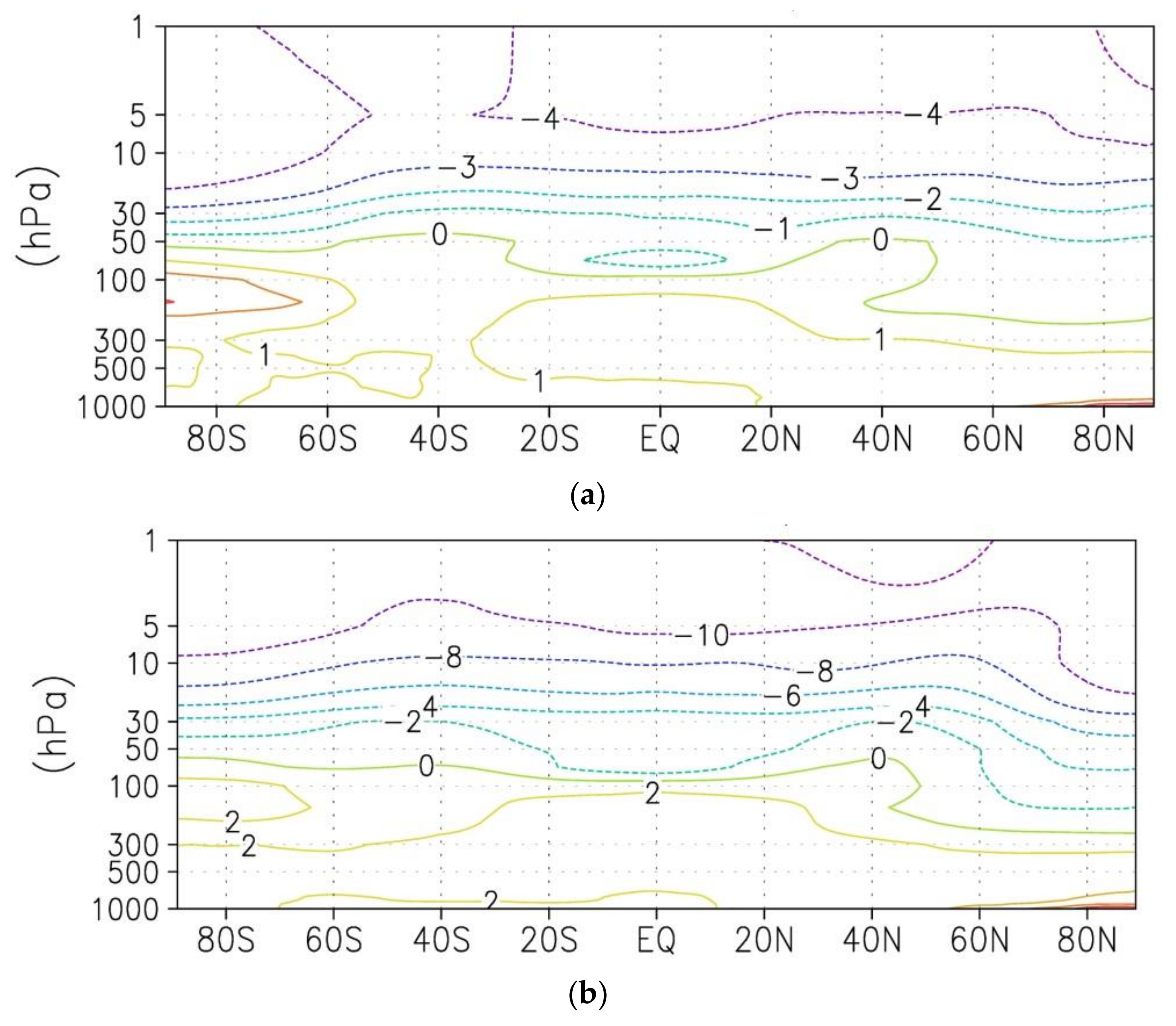
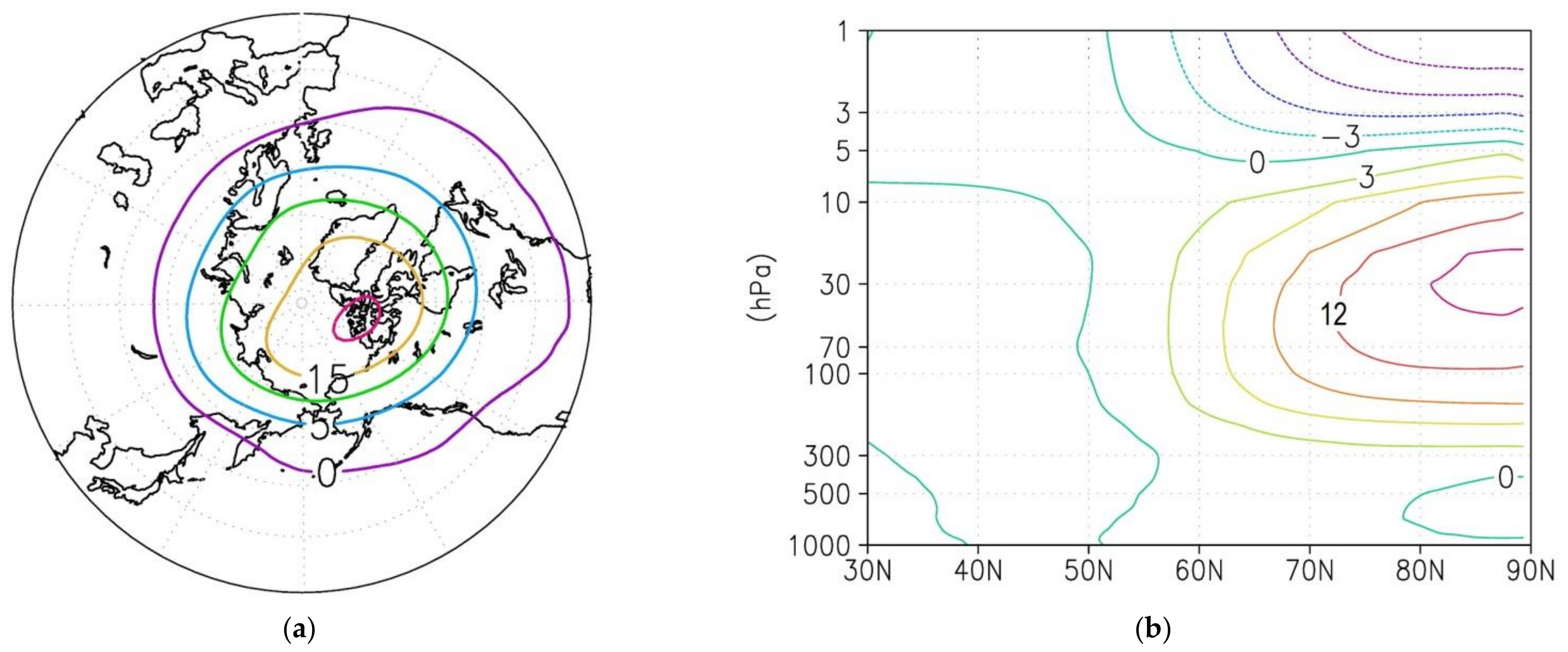
Differences of zonal mean temperature in January between two periods 2081–2100 and 2016–2035 are presented on Figure 1a,b. Under a moderate scenario, the temperature decrease by the end of the 21st century ranges from ~1 K in the lower stratosphere to ~4 K in the upper stratosphere. The severe scenario is accompanied by temperature decrease from ~1 K at the lower stratosphere to ~12 K at the upper stratosphere. Under severe scenario tropospheric temperature increase is also stronger. Analysis of changes in the seasonal variation of the stratospheric temperature in the polar region (70° N–90° N) showed that under the moderate scenario, the largest temperature decrease is observed in March in the middle stratosphere at 30 hPa and reached the value of 4 K, under the severe scenario—the value of 8 K in February (Figure 1c,d).
Stratospheric temperature decrease leads to a strengthening of the mean zonal wind over high latitudes, with averaging over December–February under the moderate scenario by more than 2 m/s and under severe scenario by 8 m/s.
3.2. Planetary Wave Activity
Planetary waves propagating from the troposphere into the stratosphere have a significant effect on the strength and persistence of the stratospheric polar vortex, and thereby, determine the character of the ozone layer destruction. With enhanced upward wave activity significant ozone destruction is not observed in the Arctic stratosphere (e.g., [48]). A decrease in stratospheric temperature is accompanied by a strengthening of wave activity propagation.
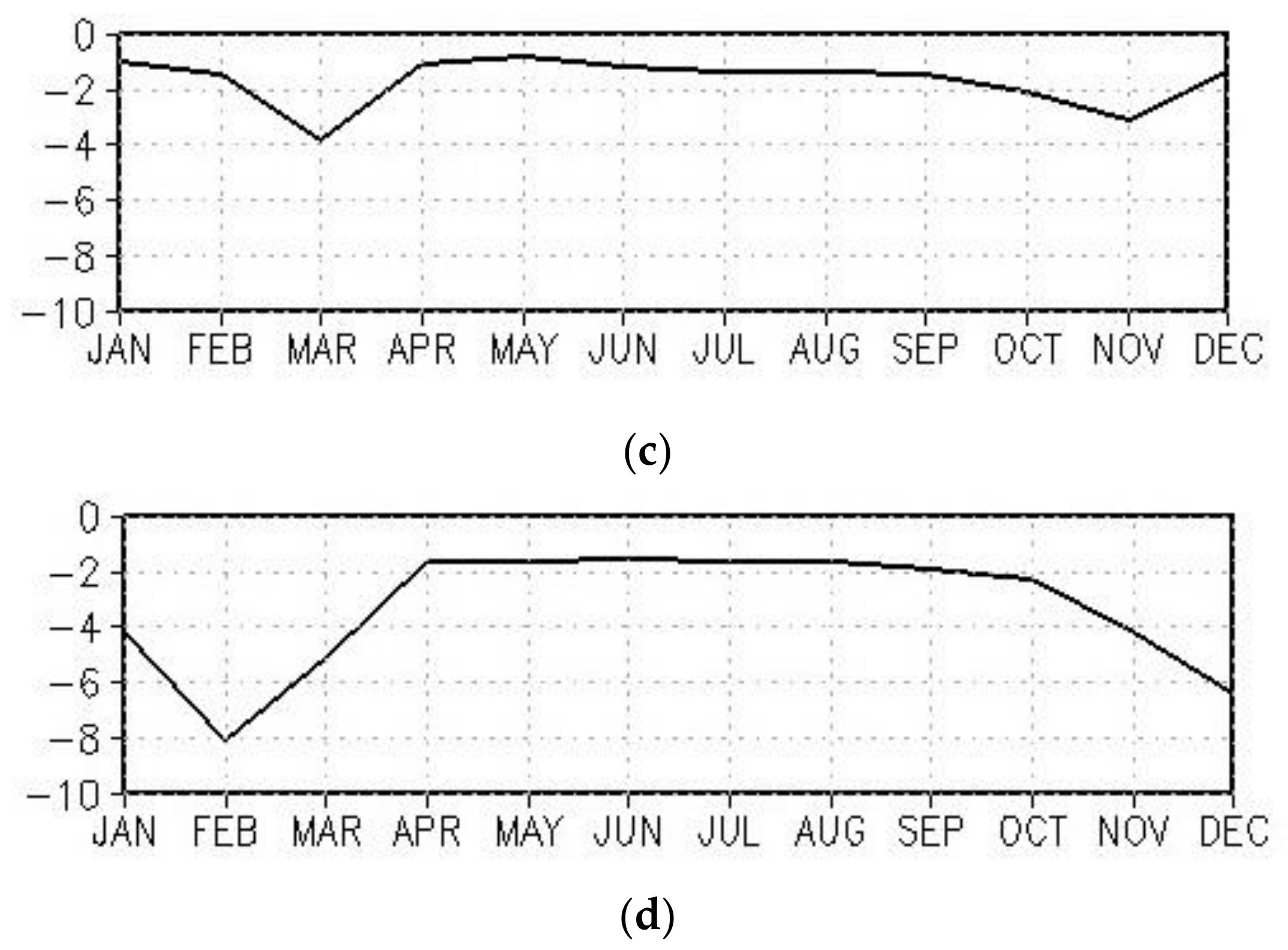
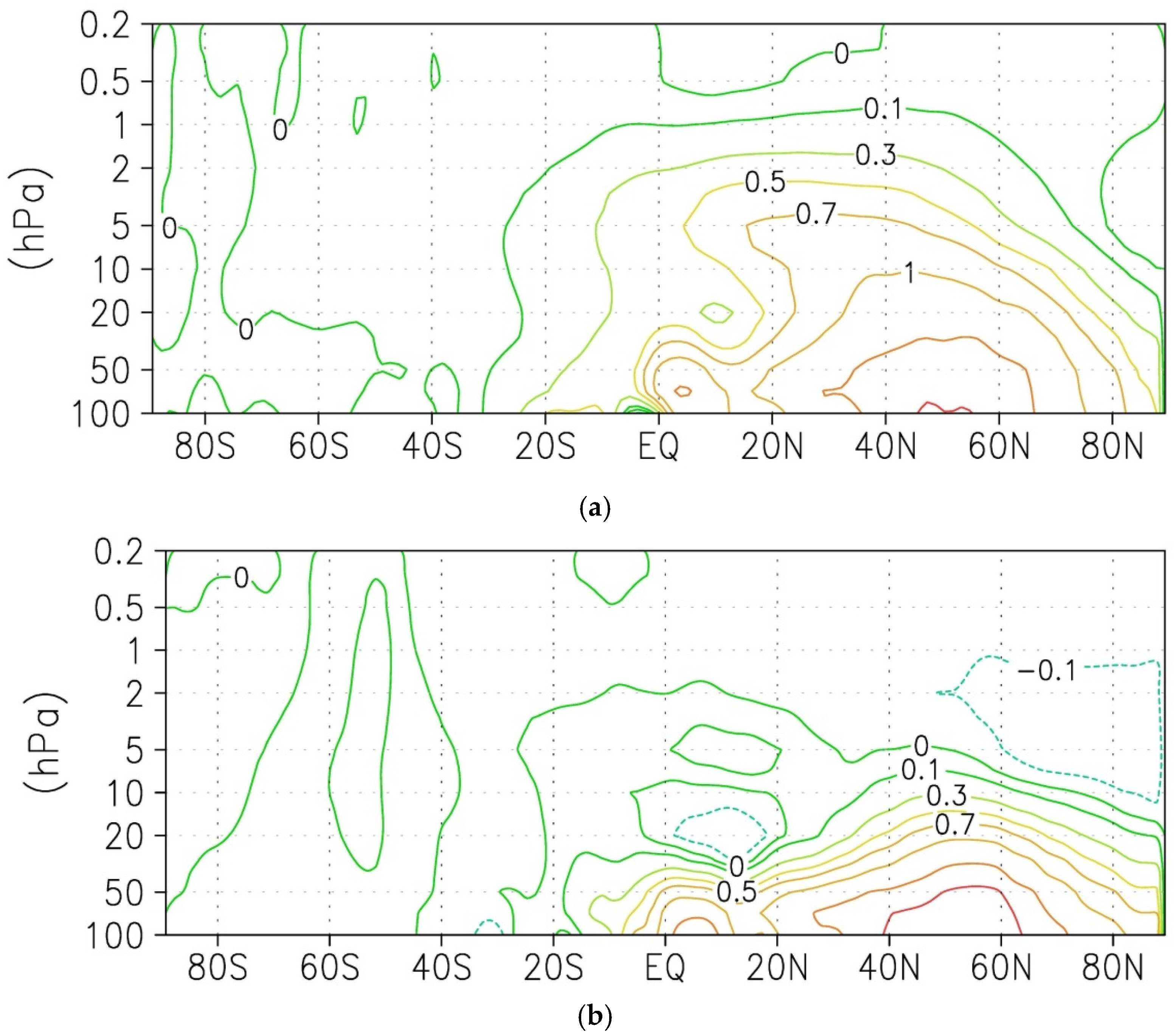
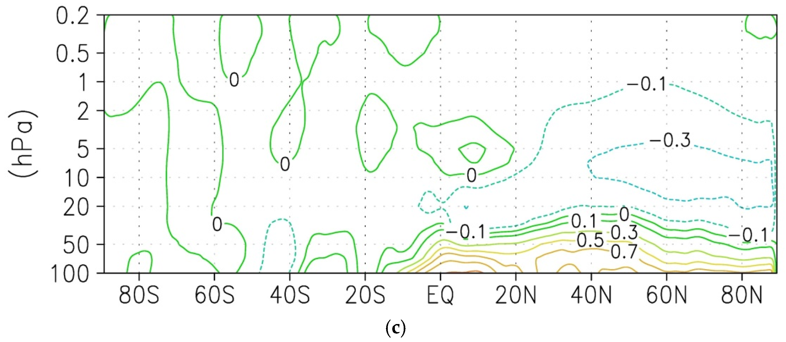
The change in the zonal mean meridional heat flux , where v′ and T′ are deviations of meridional wind and temperature from zonal mean values, was analyzed (Figure 2a,b). According to both scenarios, an increase in upward wave activity propagation in stratosphere is observed by the end of the 21st century. This increase is maximized in the upper stratosphere at 60° N–70° N. At the same time, a decrease of heat flux is observed at high latitudes in the lower stratosphere.
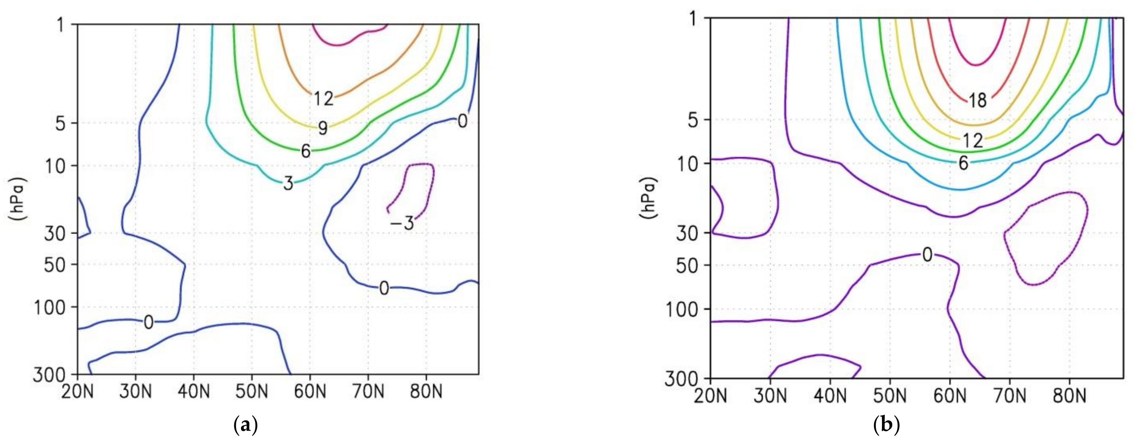
The change in the amplitudes of stationary planetary waves with zonal numbers 1 and 2 (hereafter SPW1 and SPW2), which dominate over extratropical latitudes in the winter stratosphere, was analyzed (Figure 3). In a moderate scenario, the SPW1 amplitude increases in the upper stratosphere in the region of 60° N–70° N by ~100 gpm (~15%), while for SPW2, the amplitude difference does not exceed 20 gpm. In the severe scenario, the SPW1 increase is more than 250 gpm (~25%) in the upper stratosphere at the 60° N–70° N. For SPW2, the increase is more than 40 gpm in the middle stratosphere and the attenuation with maximum nearby 40° N is ~20 gpm in the upper stratosphere. Possibly, the strengthening of the mean zonal wind in the extratropical stratosphere contributes to the enhancement of SPW1 in the middle and upper stratosphere.
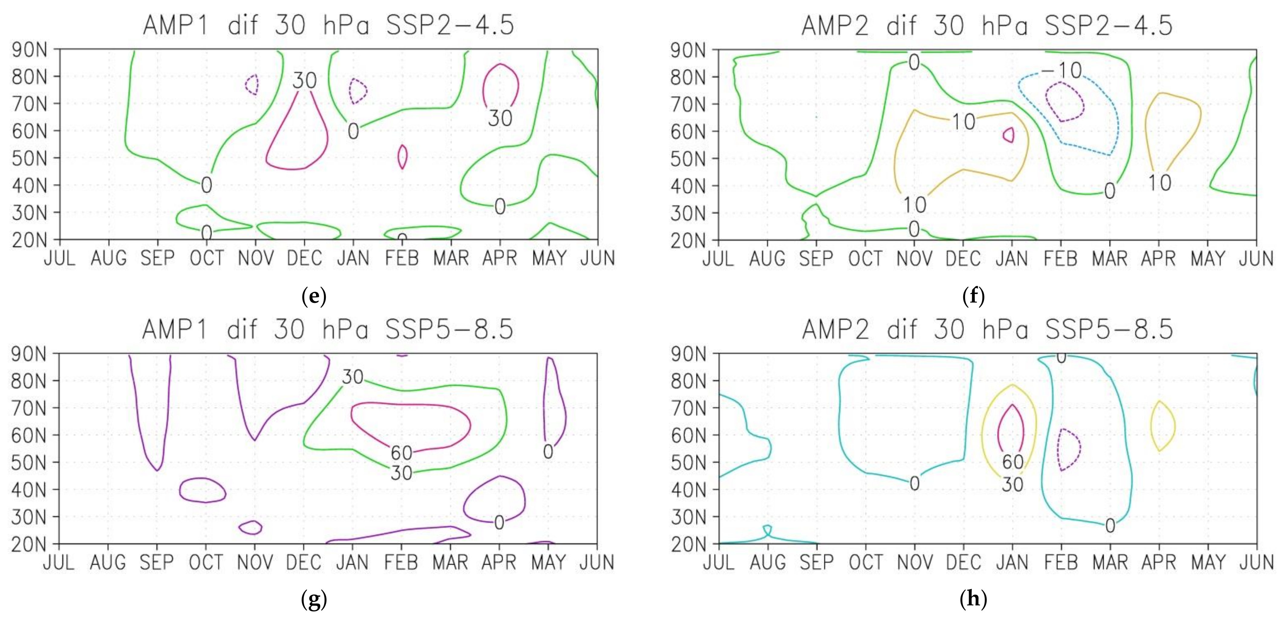
As our study is focused on a difference of dynamical processes in the lower and middle boreal stratosphere, the difference of the seasonal cycle of SPW1 and SPW2 at pressure level 30 hPa was analyzed (Figure 3e–h). In a moderate scenario, the difference of the SPW1 amplitude between the periods of 2081–2100 and 2016–2035 is about 20–40 gpm from November till April. Difference of SPW2 amplitude is less than 20 gpm during the whole winter season (Figure 3e,f). In the severe scenario, this difference for SPW1 has a maximum value in February, while this was in January, near 60° N, for SPW2. In both cases, the maximum value exceeds ~80 gpm (Figure 3g,h). A slight weakening of the SPW2 amplitude in February–March should be noted.
Overall, maximum strengthening of SPW1 occurs in the upper stratosphere at high latitudes at the end of 21st century and it is more pronounced in the severe scenario. SPW2 increased in the lower–middle stratosphere, and this increase is also stronger in the severe scenario than in the moderate. The difference of the wave activity between winters with the coldest and warmest Arctic stratospheric polar vortex will be analyzed further.
3.3. Sudden Stratospheric Warming
In the moderate scenario, 37 major SSW events were identified (i.e., with a frequency of ~0.4 per year), under the severe scenario: 27 (~0.3 per year). Earlier, in five historical simulations of the INM CM5 for the modern climate from 1965 to 2014, the mean major SSW frequency ~0.4 per year was revealed [33]. Thus, no significant change in the frequency of the major SSW events has been detected during the 21st century. This result is consistent with the estimates obtained in the analysis of moderate and severe scenarios of more than 30 climate models of CMIP5/6 simulations, including the INM CM5, where no significant changes in major SSW characteristics relative to the modern climate were revealed [49].
It is important that some SSW events that do not satisfy the definition of the major ones approved by the World Meteorological Organization (change in the direction of the zonal wind at 60° N and 10 hPa) can have a significant impact, for example, on the formation of conditions for the stratospheric ozone destruction, such as minor SSW in the Arctic in early January 2015 [50]. In this regard, in recent years, the need to improve the definition of the major SSW events has been discussed [51]. Possibly, the mean zonal wind reversal at higher levels should be considered [52].
3.4. Final SSW Dates
In both moderate and severe scenarios, the analysis of INM CM5 output data shows a slight positive trend in the Final SSW dates to later dates by the end of the 21st century. However, both trends are insignificant.
In the moderate scenario, the Final SSW date averaged over the entire period from 2016 to 2100 is March 18, while in the severe scenario this is March 21. Most of the Final Warming events are observed in March. The earliest Final SSW dates were revealed in late January and early February, and the latest in late April and early May. In the moderate scenario, the Final SSW date averaged over the first 20 years (from 2016 to 2035) is March 17 and averaged over the last 20 years (2081–2100) is March 18, and March 18 and March 20 under the severe scenario respectively.
Therefore, significant changes of Final SSW dates during the 21st century were not revealed in both scenarios. Earlier, the analysis of calculations of the CMIP5/6 project models, including the INM CM5 and multi-model average values, also did not reveal significant changes in the parameters of the Final SSW in the Northern Hemisphere. Only for the severe scenario, a delay by ~5 days was detected [53].
Planetary waves can affect the Final SSW dates—such early events are accompanied by an increase in the amplitude of the dominant SPW1 in the stratosphere. During late Final SSW wave activity is weaker and this event is caused by seasonal heating of the middle atmosphere [36].
The revealed significant linear relationship between the dates of Final SSW and the amplitudes of SPW1 in March at a pressure level of 10 hPa (correlation coefficient is −0.62) in the ERA-Interim reanalysis data from 1980 to 2017, as well as in three out of five calculations of the INM CM5 for the period from 1965 to 2015 with a correlation coefficient from −0.29 to −0.53 [37].
For the future climate under the moderate and severe scenarios, the correlation coefficients between the dates of Final SSW and the amplitudes of SPW1 in March at a pressure level of 10 hPa were −0.08 and −0.17, respectively, and at a significance level of 95% according to Student’s t-test, these correlations are insignificant.
3.5. Interannual Variability of Arctic Stratospheric Circulation
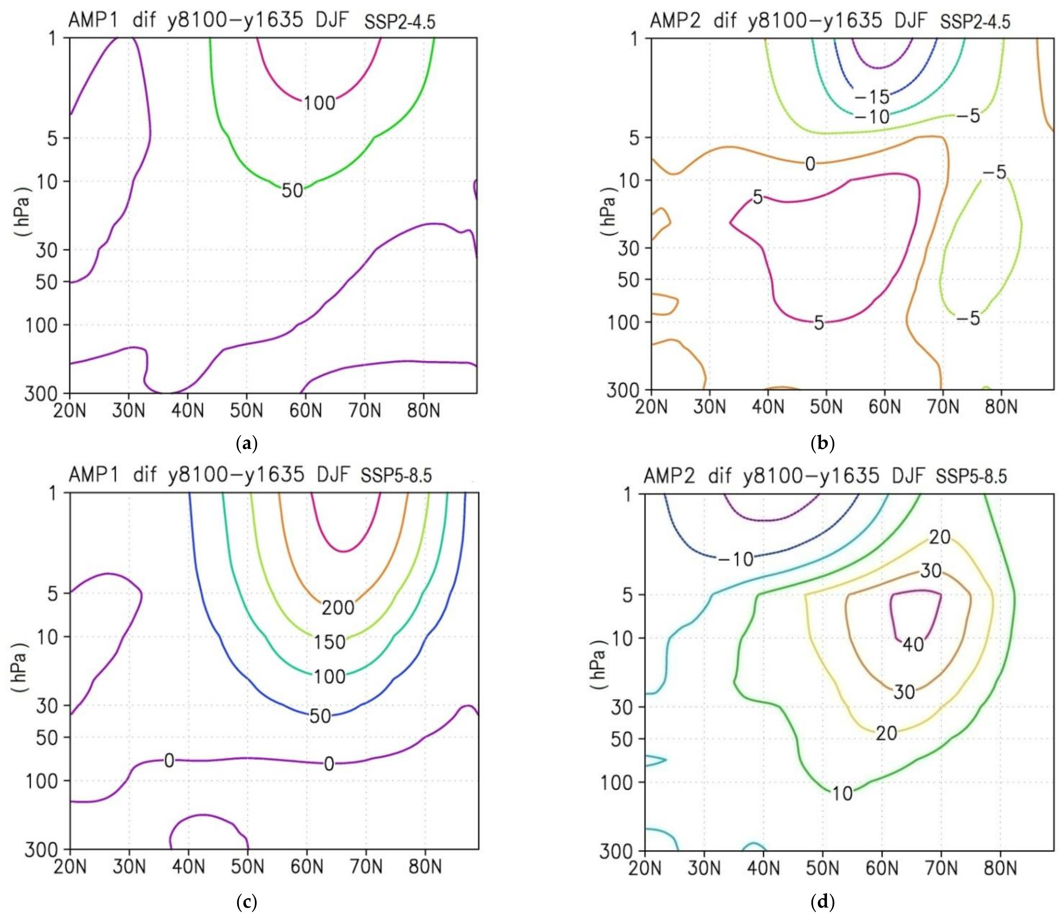
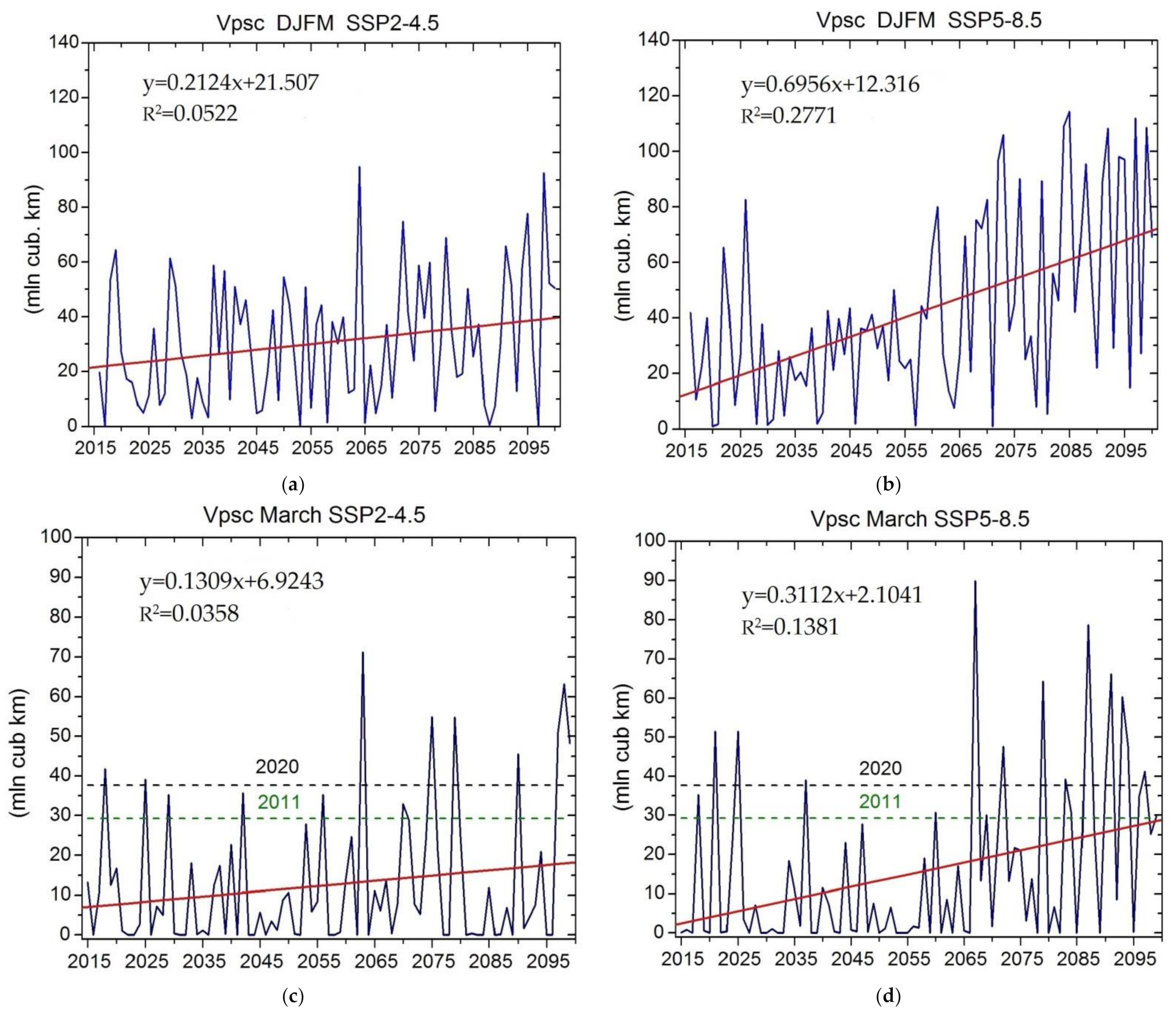
Model calculations for both scenarios indicate a decrease in temperature inside the Arctic stratospheric polar vortex by the end of the 21st century by 2–6 K. Analysis of the Vpsc values calculated for the range of the lower stratosphere heights from 390 K to 590 K (~120–~30 hPa) from December to March indicates their growth by the end of the 21st century for the moderate and, especially, for the severe scenario (Figure 4a,b). This increase is most likely in January and February. With an increase in the mean Vpsc value by the end of the century, their variance or interannual variability also increases. The obtained estimates agree with the results of the calculations analysis of the CMIP6 project models, including the INM CM5, as well as four chemistry climate models [19]. Analysis of the calculated Vpsc showed that by the end of the 21st century, their average volume increases in winter, and most strongly in January–February. The period when PSC are formed also increases; for example, they are formed throughout the whole winter in the late 21st century in a severe scenario. The maximum values of the Vpsc also increase in cold winters and it is consistent with others results [19].
An increase in the Vpsc by the end of the 21st century is also observed in March, when the greatest destruction of stratospheric ozone usually occurs in the Arctic (Figure 4c,d). Trends are also significant for both moderate and severe scenarios. The maximum value of the Vpsc in March for the entire analyzed period in the moderate scenario is ~71 million km3 (winter of 2063 year) and ~90 million km3 in the severe scenario (winter of 2068 year). For comparison, according to the MERRA-2 reanalysis, the Vpsc in March 2011 and 2020, when the ozone depletion in the Arctic stratosphere was the greatest over all period of observations, reached ~29.3 and ~37.6 million km3, respectively.
With a significance level of 95% according to Student’s t-test, the trends of Vpsc averaged over December–March and separately for March in the Arctic during the 21st century are significant for both moderate and severe scenarios.
In contrast to [19], in addition to the vertical profiles of H2O and HNO3 distribution corresponding to the modern climate and necessary for calculating the Vpsc, vertical profiles from the calculations with the chemistry climate model (CCM) SOCOL3 [54] for the moderate and severe scenario of future climate were used. According to simulations of this model, the concentrations of these gases will increase in the Arctic stratosphere by the end of the 21st century. It is possible to calculate the critical temperature of the PSC type I formation (Tnat) according to the formula from [55] for different profiles of these gases.
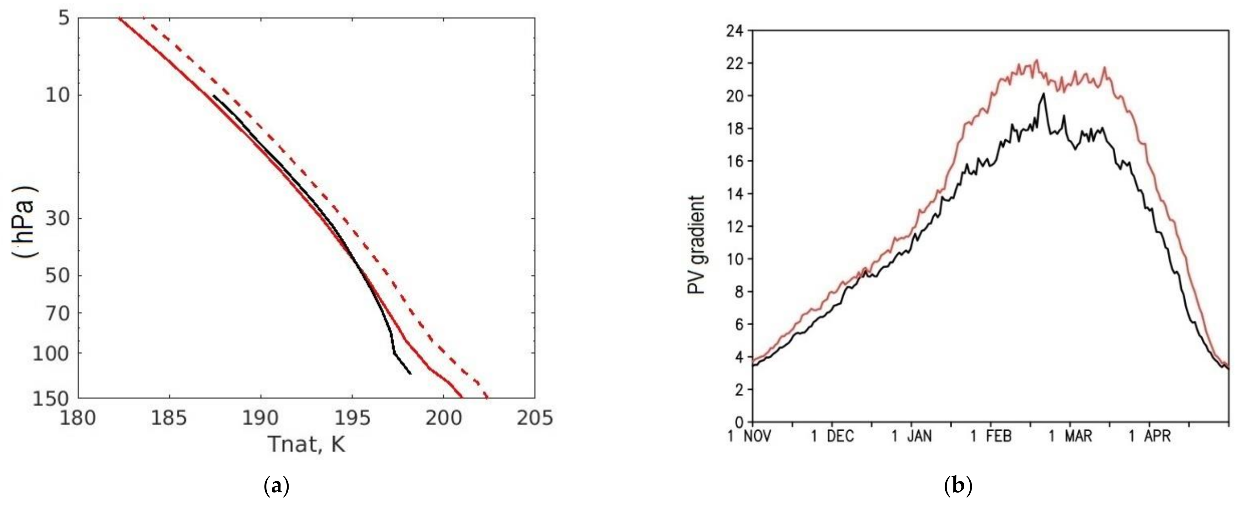
Figure 5a shows the profiles of the critical temperature Tnat according to [38], as well as those calculated from the CCM SOCOL3 for the beginning and the end of the century. It can be concluded that the critical temperature of the PSC type I formation will increase by 1–1.5 K by the end of the 21st century. When calculating with the new critical temperature, the Vpsc should also increase.
The isolation of the stratospheric polar vortex depends on the meridional gradient of the wind speed in atmospheric jets. If we calculate the maximum meridional potential vorticity gradient according to [38] (Figure 5b), it turns out that it increases at the end of the 21st century in the middle stratosphere in February–March by 20%, which corresponds to a decrease in effective diffusivity at the vortex boundary and to an increase in its isolation [56].
Analysis of the temperature dispersion inside the stratospheric polar vortex showed that in the lower stratosphere, it decreases in March and increases in January (Figure S2). Thus, the region with the maximum variance is shifted to an earlier period. In a moderate scenario, the characteristics of the stratospheric polar vortex change in a similar way, but their differences at the beginning and the end of the 21st century are less pronounced.
3.6. Stratospheric Meridional Circulation
In the troposphere, the meridional circulation is mainly characterized by the Hadley cells in the tropics and the Ferrel cells (northward and southward of the Hadley cells). According to the calculations of the INM CM5, weakening of the Hadley cells in both hemispheres is expected, as well as its upward propagation and expansion, especially in the Northern Hemisphere by the end of the 21st century [26].
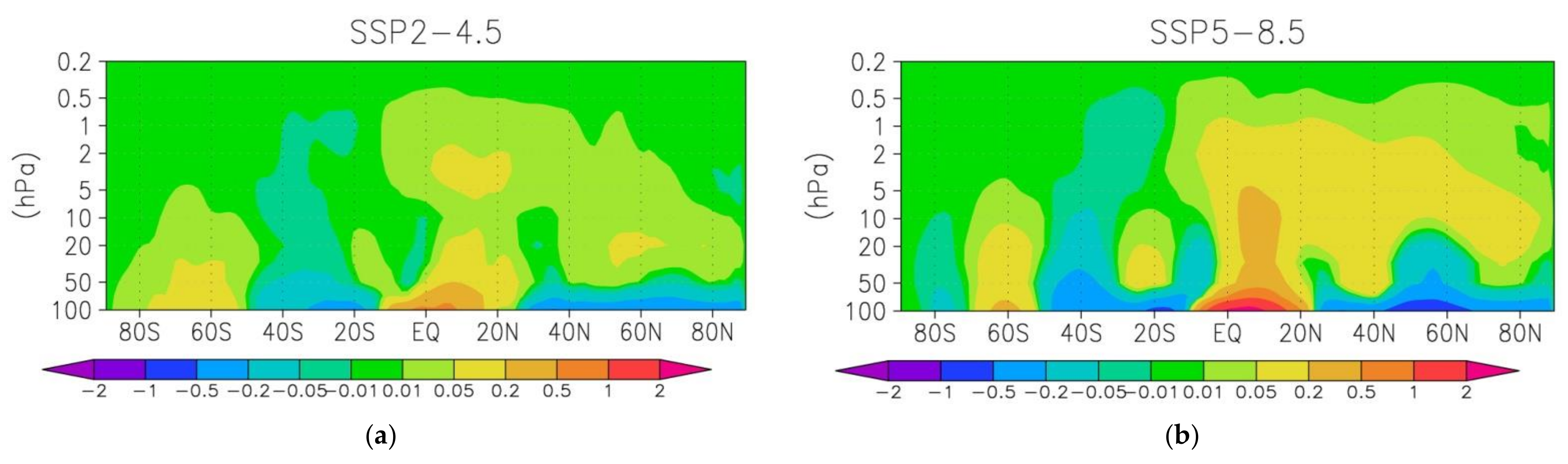
In the stratosphere, by the end of the 21st century, there will be an increase in upward transport in the equator–northern tropics and downward transport in high latitudes of the Northern Hemisphere in winter (Figure 6a,b). These changes are stronger in the severe scenario. The revealed increase in the meridional circulation of the stratosphere leads to a decrease in the average “age” of the air, as well as due to the intensification of downward movements to an increase in the Arctic stratosphere temperature. Positive values of stream function correspond to a clockwise motion.
3.7. Composite Analysis
The greatest difference in temperature between the “warm” and “cold” winters in the Arctic lower stratosphere is observed in January: in the “warm” winters, it is higher by more than 18 K (Figure 7a). For the zonal mean temperatures averaged over December–February, the maximum difference is more than 15 K in the region of 70° N–90° N nearby 30 hPa (Figure 7b), while the zonal mean zonal wind is more than 30 m/s near 60° N with a pressure level of 10 hPa.
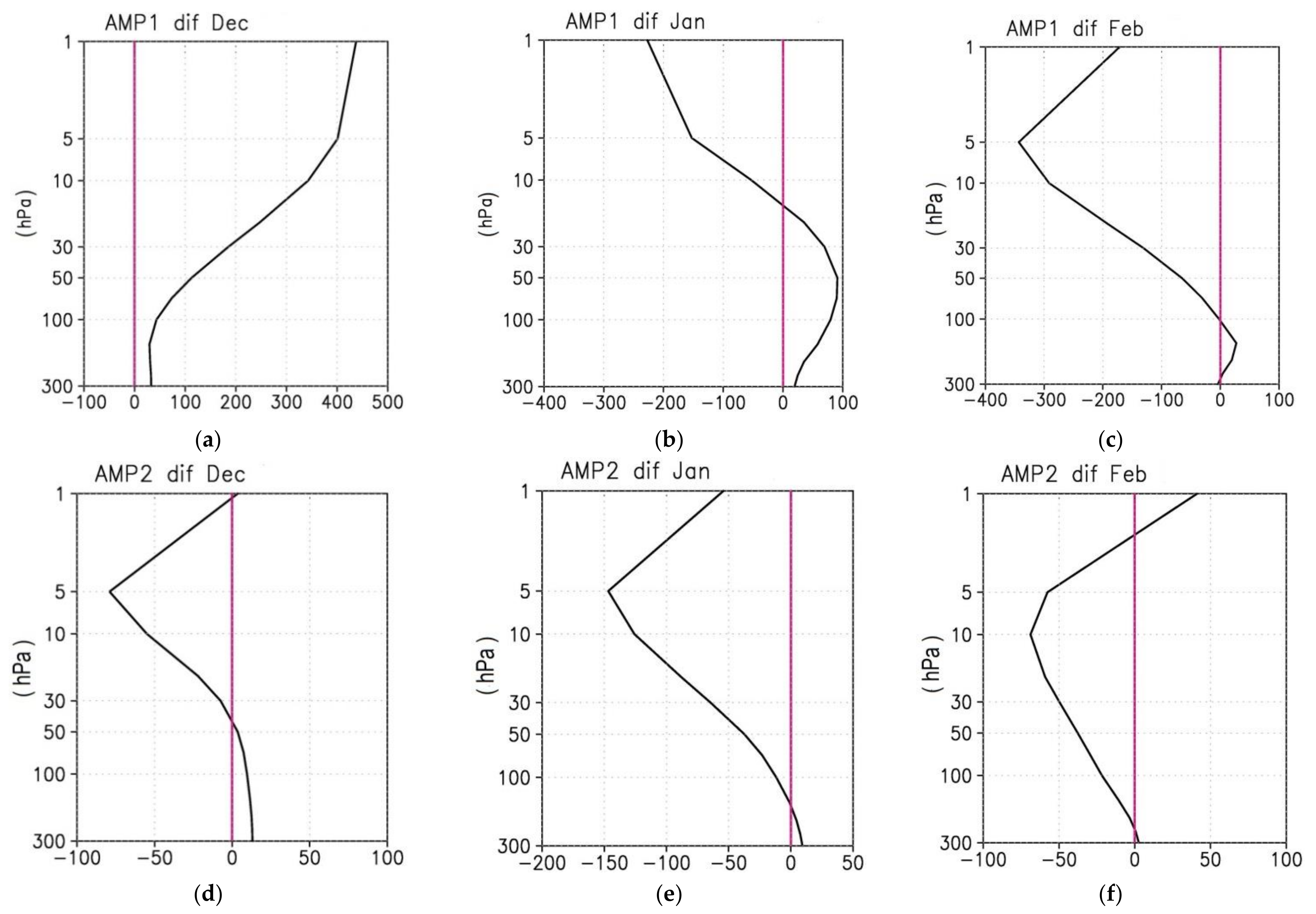
The changes in the amplitude of the dominant in extratropical stratosphere stationary planetary wave number 1 and 2 (SPW1 and SPW2) for the winter months were analyzed. If in December the amplitude of SPW1 is greater in the “warm” winters than in the “cold” winters, then in January the amplitude of this wave is slightly higher only in the lower stratosphere (by ~100 gpm), while this is less in the middle stratosphere (up to ~250 gpm) and in February (up to ~350 gpm) than in the “cold” seasons (Figure 8a–c). The SPW2 amplitude in the “warm” winters is less in the lower and middle stratosphere than in the “cold” winters: the largest difference is ~150 gpm near pressure levels of 5–10 hPa in January, and is about 60–70 gpm in December and February (Figure 8d–f).
Unlike SPW2, a slow downward propagation of the SPW1 difference from December to February is observed.
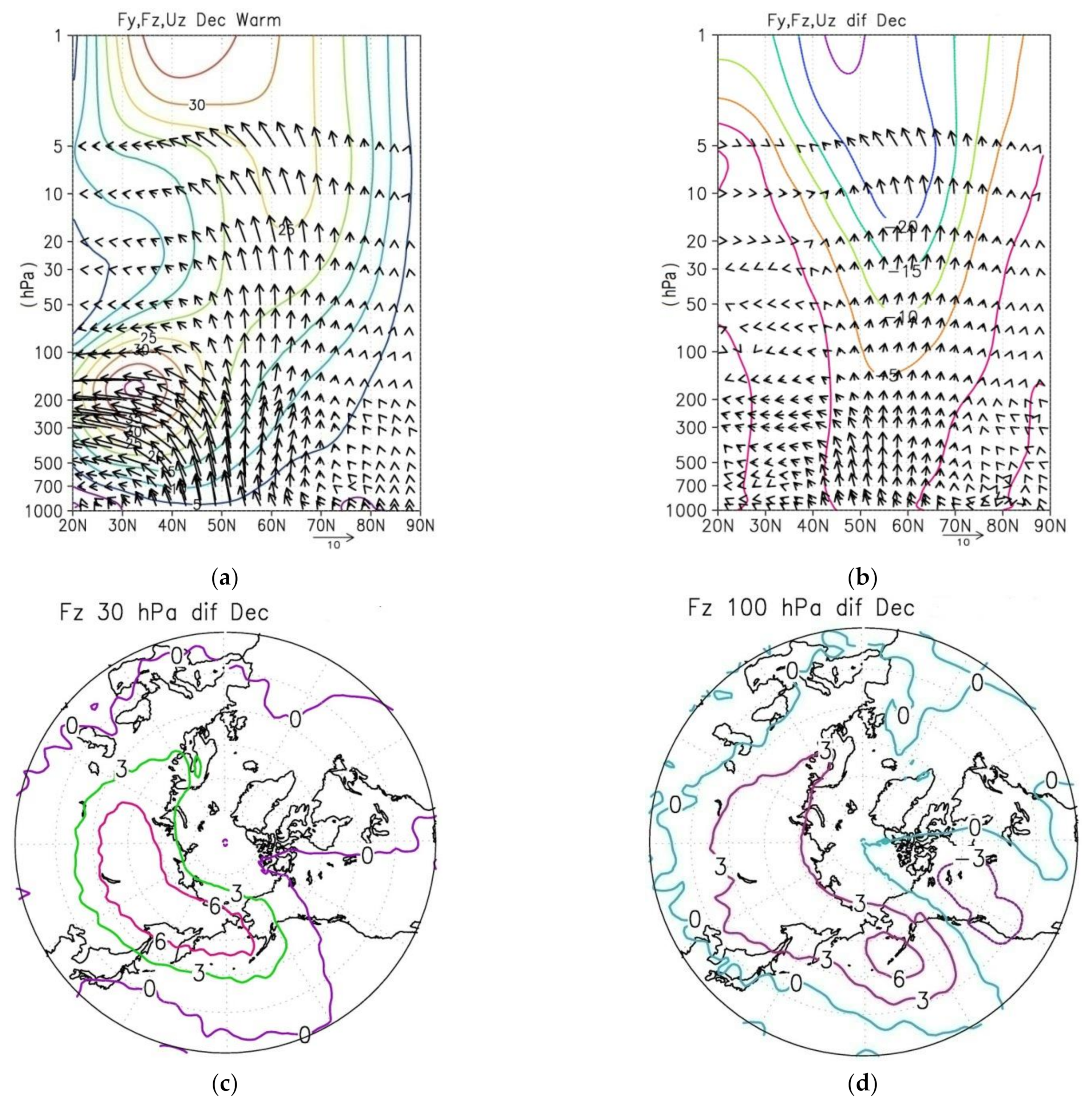
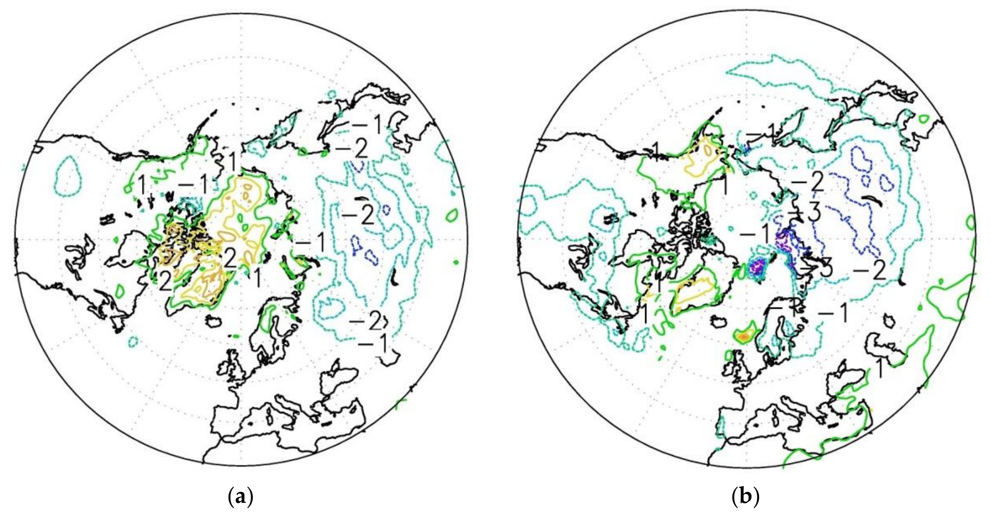
Furthermore, the analysis of the planetary wave propagation was carried out using the Plumb flux vectors. In Figure 9a, the zonal mean values are shown of the latitudinal and vertical components of the Plumb flux vector (Fy, Fz) and the zonal mean wind in December for the “warm” winter composite. Wave activity propagation from the troposphere to the stratosphere in the region of 40° N–70° N is clearly seen. Propagation to low latitudes dominates in the middle stratosphere. A comparison between the composites shows that in the warm winters, the propagation of wave activity is stronger in the early winter, especially in the lower and middle stratosphere (Figure 9b). This is also confirmed by the stereographic projections of the vertical component of the Plumb flux vector differences for the middle and the lower stratosphere (at 30 hPa and 100 hPa) between the composites: a greater upward propagation of wave activity can be seen over the eastern part of Northern Eurasia in December in the warm winters (Figure 9c,d).
The greatest upward propagation of wave activity is observed over the North- Eastern Eurasia for both the “warm” and “cold” winters, which corresponds to the climatic features of the wave activity longitudinal distribution according to observational data (e.g., [57,58,59]).
A stronger upward propagation of wave activity in the stratosphere over Northern Eurasia in December corresponds to a weaker stratospheric polar vortex on average for the entire winter season. This is in accordance with the results of a wave activity analysis [58] performed using the Japanese 55-year Reanalysis (JRA55) data since 1958 [60].
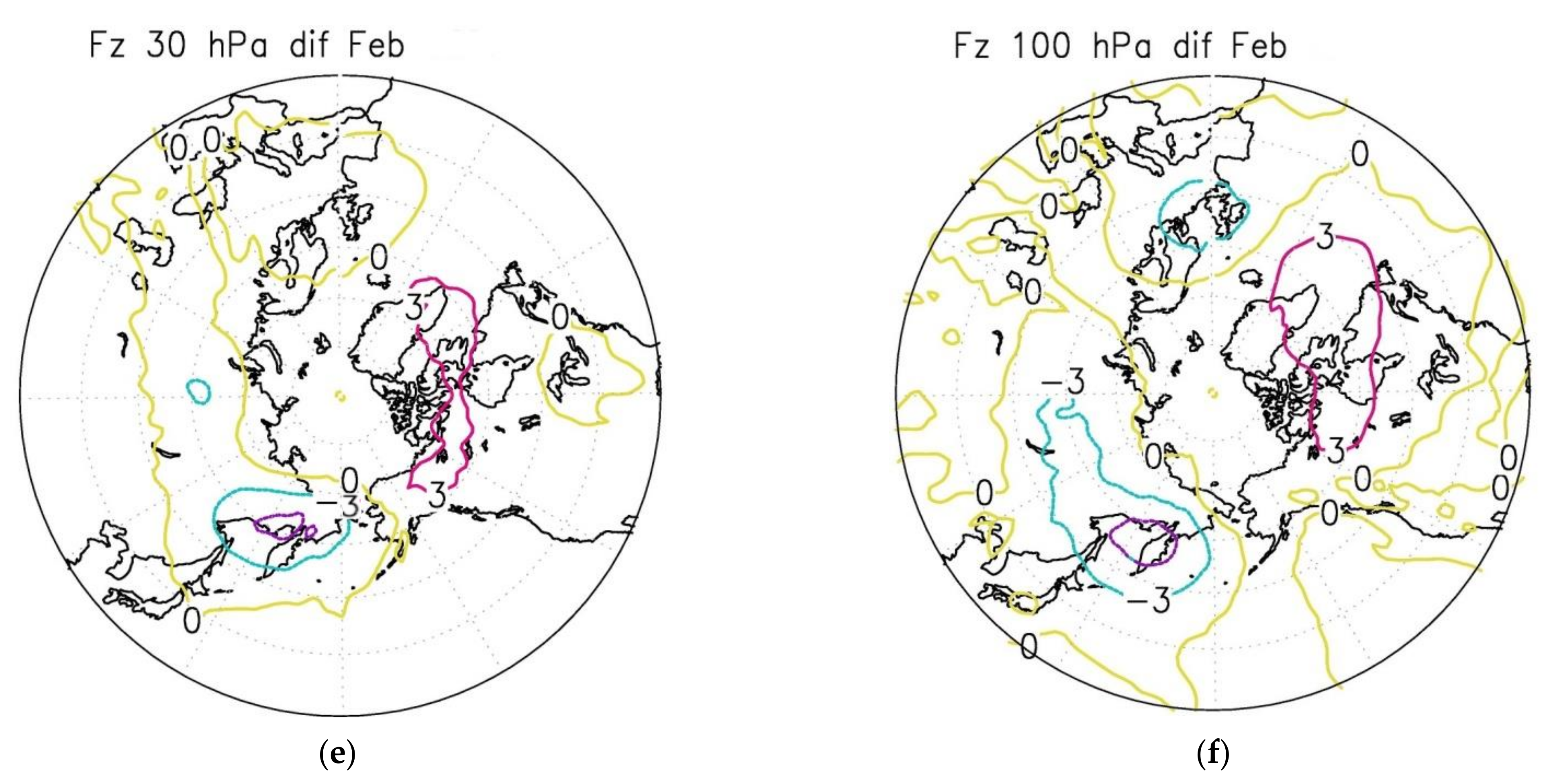
Interestingly, in January–February, a stronger wave activity propagation from the troposphere into the stratosphere as well as from the lower stratosphere to the upper over the east of Northern Eurasia was revealed in the “cold” winters. This is in agreement with [59]. As an example, the difference in the vertical component of the Plumb flux vector Fz in February between the “warm” and “cold” winters is plotted on Figure 9e,f. The area of positive values of the differences over the north of North America indicates the possibility of a stronger downward reflection of wave activity (typical for this region) in the “cold” winters.
For comparison altitude-latitude cross sections of Plumb vectors Fy, Fz and zonal mean zonal wind difference between “warm” and “cold” winters in November, January, and February are present in Figure S3 and vertical component of Plumb vectors Fz difference between “warm” and “cold” winters at pressure level 30 hPa and 100 hPa for the same months are presented in Figure S4.
Simultaneously with the strengthening of the wave activity propagation from the troposphere into the stratosphere, an increase in the residual meridional circulation is observed, the greatest of which in December in the entire range of heights of the stratosphere, including the upward transport in the middle latitudes and the downward transport in the polar region (Figure 10a). A weaker difference of residual meridional circulation between composites is observed in January and February (Figure 10b,c).
The beginning of the “warm” winter seasons (November–December) is characterized by lower temperatures of the lower troposphere and on the surface in the south of Siberia—Central Asia with a maximum near Lake Baikal by 1–2 K (Figure 11a). This is consistent with the results of [59], where it was shown that the region of lower temperature at the beginning of winter near Lake Baikal characterizes, on average, winter seasons with a weaker stratospheric polar vortex. This area near Lake Baikal is the part of the Scandinavian wave train pattern [61,62], with higher pressure over Western Europe—Scandinavia—and lower over the North Atlantic. Coupling between cold Siberia anomalies and weakening of Arctic stratospheric polar vortex during late autumn to early winter was revealed in ERA-Interim reanalysis and European Centre for Medium-Range Weather Forecasts (ECMWF) seasonal forecast system data [63].
The “warm” winters in the Arctic stratosphere are accompanied by lower temperatures in North-Eastern Eurasia in March-April compared to the “cold” winters: up to 2–3 K (Figure 11b). This result is in qualitative agreement with the difference in surface temperature between composites composed of seasons with high and low ozone in the lower stratosphere from ensemble calculations of the Whole Atmosphere Community Climate Model (WACCM4) for the period from 1985 to 2005 [64].
A similar analysis of the differences between the “warm” and “cold” winter composites obtained using mean values of the least and largest Vpsc of 10 winters was carried out for the model simulation on moderate scenario of GHG growth. For the zonal mean temperatures averaged over December–February, the maximum difference between the composites is, as for the severe scenario, more than 15 K in the region of 70° N–90° N near 30 hPa. As well as for the severe scenario, at the beginning of the winter season (November–December), a higher wave activity propagation and lower surface temperatures in Northern Eurasia by 1–2 K in November–December and by 3–4 K in March-April are observed in the “warm” winters compared to the “cold” winters. The enhancement of the meridional residual circulation for the “warm” winters as compared to the “cold” winters is weaker than under the severe scenario.
4. Discussion and Conclusions
Obviously taking into account feedback and numerous interactions between dynamical and chemistry processes in the Arctic stratosphere (reinforcement of polar vortex by ozone destruction, possible stratospheric humidity increase due to climate change, etc.), investigations of expected stratospheric dynamics changes have an advantage when they use climate models with interactive chemistry. However, mainly due to very high computational cost of such simulations, the majority of CMIP6 climate models (including INM CM5) do not include interactive chemistry. The other interesting point that needs further research consists of the possible changes of smaller waves as compared to stationary planetary wavenumber 1–2 and gravity wave parameters associated to GHG growth and how this affects the stratospheric circulation.
The results obtained in our study indicate the possibility of the formation of conditions for the strong destruction of the ozone layer in the Arctic stratosphere in some winters after the 2050s, especially under a severe scenario of GHG growth. It is consistent with the results of the analysis of simulations of 20 climate models of the CMIP6, including four CCMs [19]. Even considering the expected decrease in ozone-depleting substances in the atmosphere, the formation of such conditions (especially in March) can lead to significant destruction of the stratospheric ozone.
We calculated Vpsc using vertical profiles of H2O and HNO3 corresponding to the modern climate. Additionally, using data from simulations with CCM SOCOL3 for the moderate and severe scenarios, we obtained profiles for these gases at the end of the 21st century. Then, we calculated the PSC formation critical temperatures corresponding to these profiles and predicted their growth by 1–1.5 K. This will lead to a stronger increase of Vpsc by the end of the 21st century than when we use current critical temperatures for Vpsc calculation.
Our other estimates (the remaining Major SSW frequency and the distribution of the Final SSW dates, strengthening of planetary wave activity and meridional circulations) are also consistent with simulations of some other CMIP6 climate models. However, a difference in the simulations of the dynamics of the Arctic stratosphere and estimates of its future changes between CMIP6 models is known [27,65].
The obtained estimates of surface temperature and planetary wave propagation differences between winters with the smallest and largest winter mean Vpsc might be verified by the analysis of more model simulations and comparison with simulations using interactive chemistry that is important for stratosphere–troposphere coupling [66].
Overall, analysis of simulations of the climate model INM CM5 for the moderate (SSP2-4.5) and severe (SSP5-8.5) scenarios of GHG growth allows us to formulate the following conclusions:
- By the end of the 21st century, in comparison with its beginning, in the winter stratosphere, there will be a decrease in the zonal mean temperature from about −1 K in the lower to −4 K in the upper stratosphere (from ~5 hPa to 1 hPa, ~35–~50 km) under the moderate scenario and, accordingly, from −1 K to −11 K under the severe scenario.
- The strengthening of wave activity propagation and a stationary planetary wave number 1 in the middle and upper stratosphere (especially in severe scenario) is expected.
- No changes in the frequency of the Major SSW events and in the distribution of the Final SSW dates in the Northern Hemisphere were revealed in both scenarios.
- By the end of the 21st century, a strengthening of the residual circulation in the upper stratosphere of the Northern Hemisphere in winter was revealed, which characterizes the Brewer-Dobson meridional circulation. Under a severe scenario, this strengthening is stronger.
- By the end of the 21st century, an increase of winter mean Vpsc and monthly March values in the Arctic stratosphere and the strengthening of the interannual variability of this parameter (especially under the severe scenario) were revealed. The period of PSC formation is increasing. For the severe scenario, they can form during the whole winter at the end of the century. The maximal Vpsc values are also increased.
- Maximal PV gradient increases in the middle stratosphere in February–March by 20% by the end of the 21st century, which could be related with a decrease in effective diffusivity at the boundary of the Arctic stratospheric polar vortex or with an increase of its isolation.
- Composite analysis of 10 winters with the smallest and largest Vpsc values shows that in the warm winters, a strengthening of wave activity propagation from the troposphere into the stratosphere in December is observed. However, this propagation may be stronger for colder winter seasons in January–February. Near surface temperatures in Central Asia and southern Siberia are expected to be 1–3 K lower in November–December in the “warm” winters (i.e., with a lower winter mean Vpsc value).
Finally, an interesting point that follows from our study is the strengthening of the Arctic stratospheric polar vortex in the lower stratosphere and planetary wave activity in the late 21st century. We suppose that the main reason of the Arctic polar vortex strengthening is the cooling of stratosphere that is stronger in the polar region. At the same time, strengthening of westerlies might favor to planetary wave activity increase. These questions will be discussed in our ongoing research.
Supplementary Materials
The following supporting information can be downloaded at: https://www.mdpi.com/article/10.3390/atmos13010025/s1, Equation S1: three-dimensional Plumb flux formula. Figure S2: Seasonal cycle of dispersion of daily average mean air temperature (K) inside Arctic stratospheric polar vortex in experiment SSP5-8.5: for the period 2015–2044 (a) and for the period 2070–2099 (b). Figure S3: Altitude-latitude cross section of Plumb vectors Fy, Fz (m2/s2) and zonal mean zonal wind difference between “warm” and “cold” winters in November (a), January (b) and February (c). Figure S4: Vertical component of Plumb vectors Fz (m2/s2) difference between “warm” and “cold” winters at pressure level 30 hPa and 100 hPa in November (a,d), January (b,e) and February (c,f) respectively. Contour intervals are 1 for November and 3 for January and February.
Author Contributions
All authors had valuable contribution in writing and editing of the text, data analysis and visualization of the results, including in providing the data of climate modeling E.M.V., analysis of stratospheric circulation changes and its tropospheric impacts P.N.V., A.I.P. and K.W. and the calculation of the Polar Stratospheric Clouds volume and the analysis of its changes S.V.K. All authors have read and agreed to the published version of the manuscript.
Funding
This research was supported by the Russian Foundation of Basic Research (grant no. 19–05-00370) (P.N.V., S.V.K., E.M.V.), (grant no. 20-55-53039) (A.I.P.), and the National Natural Science Foundation of China (grant no. 42011530082) (K.W.).
Data Availability Statement
The data of calculations of the INM CM5 for the modern and future climate are available on the CMIP6 website: https://esgf-node.llnl.gov/search/cmip6/ (accessed on 19 November 2021).
Acknowledgments
Authors are grateful to Timofei Sukhodolov from PMOD/WRC (Davos, Switzerland) and BOKU-Met (Vienna, Austria) for providing vertical profiles of H2O and HNO3 from CCM SOCOL3 simulations, Axel Gabriel from Leibniz Institute of Atmospheric Physics (Kühlungsborn, Germany) for useful comments and suggestions, and Vasilisa Vorobyeva (INM RAS, Moscow, Russia) for help with translation. In addition, the useful comments of the four anonymous reviewers are highly acknowledged. NCEP Reanalysis data were provided by Climate Prediction Center (NOAA), ERA-Interim reanalysis dataset by Copernicus Climate Change Service.
Conflicts of Interest
The authors declare no conflict of interest.
Abbreviations
| CMIP6 | Coupled Model Intercomparison Project Phase 6 |
| PSC | polar stratospheric clouds |
| Vpsc | volume of air masses with temperature below the threshold of PSC formation of the type I (Tnat) |
| BDC | Brewer-Dobson meridional circulation |
| CCM | chemistry climate model |
References
- Steiner, A.K.; Ladstädter, F.; Randel, W.J.; Maycock, A.C.; Fu, Q.; Claud, C.; Gleisner, H.; Haimberger, L.; Ho, S.-P.; Keckhut, P.; et al. Observed Temperature Changes in the Troposphere and Stratosphere from 1979 to 2018. J. Clim. 2020, 33, 8165–8194. [Google Scholar] [CrossRef]
- WMO (World Meteorological Organization). Ozone Report No. 55. Chapter 3. In Scientific Assessment of Ozone Depletion; WMO: Geneva, Switzerland, 2018. [Google Scholar]
- Randel, W.; Smith, A.; Wu, F. Stratospheric Temperature Trends over 1979–2015 Derived from Combined SSU, MLS, and SABER Satellite Observation. J. Clim. 2016, 29, 4843–4859. [Google Scholar] [CrossRef]
- Keeble, J.; Hassler, B.; Banerjee, A.; Checa-Garcia, R.; Chiodo, G.; Davis, S.; Eyring, V.; Griffiths, P.; Morgenstern, O.; Nowack, P.; et al. Evaluating stratospheric ozone and water vapour changes in CMIP6 models from 1850 to 2100. Atmos. Chem. Phys. 2021, 21, 5015–5061. [Google Scholar] [CrossRef]
- Baldwin, M.; Dunkerton, T. Stratospheric harbingers of anomalous weather regimes. Science 2001, 294, 581–584. [Google Scholar] [CrossRef] [PubMed]
- Baldwin, M.; Birner, T.; Brasseur, G.; Burrows, J.; Butchart, N.; Garcia, R.; Geller, M.; Gray, L.; Hamilton, K.; Harnik, N.; et al. 100 Years of Progress in Understanding the Stratosphere and Mesosphere. Meteorol. Monogr. 2019, 59, 27.1–27.61. [Google Scholar] [CrossRef]
- Kolstad, E.; Breiteig, T.; Scaife, A. The association between stratospheric weak polar vortex events and cold air outbreaks in the Northern Hemisphere. Q. J. R. Meteorol. Soc. 2010, 136, 886–893. [Google Scholar] [CrossRef] [Green Version]
- Nath, D.; Chen, W.; Zelin, C.; Pogoreltsev, A.; Wei, K. Dynamics of 2013 Sudden Stratospheric Warming event and its impact on cold weather over Eurasia: Role of planetary wave reflection. Sci. Rep. 2016, 6, 24174. [Google Scholar] [CrossRef]
- Vargin, P.N.; Guryanov, V.V.; Lukyanov, A.N.; Vyzankin, A.S. Arctic Stratosphere Dynamical Processes in the Winter of 2020–2021. Izv. Atmos. Ocean. Phys. 2021, 57, 568–580. [Google Scholar]
- Zülicke, C.; Becker, E.; Matthias, V.; Peters, D.; Schmidt, H.; Liu, H.-L.; Ramos, L.; Mitchell, D. Coupling of Stratospheric Warmings with mesospheric coolings in observations and simulations. J. Clim. 2018, 31, 1107–1133. [Google Scholar] [CrossRef]
- Pedatella, N.; Chau, J.; Schmidt, H.; Goncharenko, L.; Stolle, C.; Hocke, K.; Harvey, V.; Funke, B.; Siddiqui, T. How sudden stratospheric warming affects the whole atmosphere. EOS 2018, 99, 092441. [Google Scholar] [CrossRef]
- Manney, G.; Santee, M.; Rex, M.; Livesey, N.; Pitts, M.; Veefkind, P.; Nash, E.; Wohltmann, I.; Lehmann, R.; Froidevaux, L.; et al. Unprecedented Arctic ozone loss in 2011. Nature 2011, 478, 469–475. [Google Scholar] [CrossRef]
- Lawrence, Z.; Perlwitz, J.; Butler, A.; Manney, G.; Newman, P.; Lee, S.; Nash, E. The remarkably strong arctic stratospheric polar vortex of winter 2020: Links to record-breaking Arctic oscillation and ozone loss. J. Geophys. Res. 2020, 125. [Google Scholar] [CrossRef]
- Wohltmann, I.; von der Gathen, P.; Lehmann, R.; Maturilli, M.; Deckelmann, H.; Manney, G.L.; Davies, J.; Tarasick, D.; Jepsen, N.; Kivi, R.; et al. Near-complete local reduction of Arctic stratospheric ozone by severe chemical loss in spring 2020. Geophys. Res. Lett. 2020, 47, e2020GL089547. [Google Scholar] [CrossRef]
- Manney, G.; Livesey, N.; Santee, M.; Lawrence, Z.; Lambert, A.; Millan, L.; Fuller, R. Record low Arctic stratospheric ozone in 2020: MLS polar processing observations compared with 2016 and 2011. Geophys. Res. Lett. 2020, 47. [Google Scholar] [CrossRef]
- Smyshlyaev, S.P.; Vargin, P.N.; Motsakov, M.A. Numerical modeling of ozone loss in the exceptional Arctic stratosphere winter-spring of 2020. Atmosphere 2021, 12, 1407. [Google Scholar] [CrossRef]
- Tsvetkova, N.D.; Vargin, P.N.; Lukyanov, A.N.; Kirushov, B.M.; Yushkov, V.A.; Khattatov, V.U. Investigation of chemistry ozone destruction and dynamical processes in Arctic stratosphere in winter 2019–2020. Russ. Meteorol. Hydrol. 2021, 46, 597–606. [Google Scholar]
- Pascoe, C.; Lawrence, B.; Guilyardi, E.; Juckes, M.; Taylor, K. Designing and Documenting Experiments in CMIP6. Geosci. Model Dev. Discuss. 2019, 1–27. [Google Scholar] [CrossRef] [Green Version]
- Gathen, P.; Kivi, R.; Wohltmann, I.; Salawitch, R.; Rex, M. Climate change favours large seasonal loss of Arctic ozone. Nat. Commun. 2021, 12, 1–17. [Google Scholar] [CrossRef]
- Eleftheratos, K.; Kapsomenakis, J.; Zerefos, C.; Bais, A.; Fountoulakis, I.; Dameris, S.; Jöckel, P.; Haslerud, A.; Godin- Beekmann, S.; Steinbrecht, W.; et al. Possible Effects of Greenhouse Gases to Ozone Profiles and DNA Active UV-B Irradiance at Ground Level. Atmosphere 2020, 11, 228. [Google Scholar] [CrossRef] [Green Version]
- Matsuno, T. A dynamical model of stratospheric sudden warming. J. Atmos. Sci. 1971, 28, 1479–1494. [Google Scholar] [CrossRef]
- Pogoreltsev, A.; Savenkova, E.; Aniskina, O.; Ermakova, T.; Chen, W.; Wei, K. Interannual and intraseasonal variability of stratospheric dynamics and stratosphere-troposphere coupling during northern winter. J. Atmos. Solar-Terr. Phys. 2015, 136, 187–200. [Google Scholar] [CrossRef]
- Albers, J.R.; Birner, T. Vortex Preconditioning due to Planetary and Gravity Waves prior to Sudden Stratospheric Warmings. J. Atmos. Sci. 2014, 71, 4028–4054. [Google Scholar] [CrossRef]
- Ern, M.; Trinh, Q.; Kaufmann, M.; Krisch, I.; Preusse, P.; Ungermann, J.; Zhu, Y.; Gille, J.; Mlynczak, M.; Russell, J., III; et al. Satellite observations of middle atmosphere gravity wave absolute momentum flux and of its vertical gradient during recent stratospheric warmings. Atmos. Chem. Phys. 2016, 16, 9983–10019. [Google Scholar] [CrossRef] [Green Version]
- Cai, Z.; Wei, K.; Xu, L.; Lan, X.; Chen, W.; Nath, D. The Influences of the Model Configuration on the Simulation of Stratospheric Northern-Hemisphere Polar Vortex in the CMIP5 Models. Advan. Meteorol. 2017, 2017, 7326759. [Google Scholar] [CrossRef] [Green Version]
- Volodin, E.M.; Gritsun, A.S. Simulation of Possible Future Climate Changes in the 21st Century in the INM-CM5 Climate Model. Izv. Atmos. Ocean. Phys. 2020, 56, 218–228. [Google Scholar] [CrossRef]
- Ayarzagüena, B.; Charlton-Perez, A.; Butler, A.; Hitchcock, P.; Simpson, I.; Polvani, L.; Butchart, N.; Gerber, E.; Gray, L.; Hassler, B.; et al. Uncertainty in the response of sudden stratospheric warmings and stratosphere-troposphere coupling to quadrupled CO2 concentrations in CMIP6 models. J. Geophys. Res. Atmos. 2020, 125, e2019JD032345. [Google Scholar] [CrossRef]
- Volodin, E.M.; Mortikov, E.V.; Kostrykin, S.V.; Ya Galin, V.; Lykosov, V.N.; Gritsun, A.S.; Diansky, N.A.; Gusev, A.V.; Yakovlev, N.G. Simulation of modern climate with the new version of the INM RAS climate model. Izv. Atmos. Ocean. Phys. 2017, 53, 142–155. [Google Scholar] [CrossRef]
- Gerber, E.; Manzini, E. The Dynamics and Variability Model Intercomparison Project (DynVarMIP) for CMIP6: Assessing the stratosphere–troposphere system. Geosci. Model Dev. 2016, 9, 3413–3425. [Google Scholar] [CrossRef] [Green Version]
- Meinshausen, M.; Nicholls, Z.; Lewis, J.; Gidden, M.; Vogel, E.; Freund, M.; Beyerle, U.; Gessner, C.; Nauels, A.; Bauer, N.; et al. The SSP greenhouse gas concentrations and their extensions to 2500. Geosci. Model Dev. 2020, 13, 3571–3605. [Google Scholar] [CrossRef]
- Volodin, E.M.; Kostrykin, S.V. The aerosol module in the INM RAS climate model. Russ. Meteorol. Hydrol. 2016, 41, 519–528. [Google Scholar] [CrossRef]
- Vargin, P.; Volodin, E. Analysis of the reproduction of dynamical processes in the stratosphere using climate model of Institute of Numerical Mathematics, Russian Academy of Science. Izv. Atmos. Ocean. Phys. 2016, 52, 3–18. [Google Scholar] [CrossRef]
- Vargin, P.N.; Kostrykin, S.V.; Volodin, E.M. Analysis of realization of stratosphere-troposphere dynamical coupling in simulations of INM RAS climate model. Russ. Meteorol. Hydrol. 2018, 43, 780–786. [Google Scholar] [CrossRef]
- Vargin, P.N.; Kolennikova, M.A.; Kostrykin, S.V.; Volodin, E.M. Influence of equatorial and north Pacific SST anomalies on Arctic stratosphere in INM RAS climate model simulations. Russ. Meteorol. Hydrol. 2021, 46, 1–9. [Google Scholar] [CrossRef]
- Plumb, R. On the Three-Dimensional Propagation of Stationary Waves. J. Atmos. Sci. 1985, 42, 217–229. [Google Scholar] [CrossRef]
- Savenkova, E.N.; Gavrilov, N.M.; Pogoreltsev, A.I. On statistical irregularity of stratospheric warming occurrence during northern winters. J. Atmos. Sol.-Terr. Phys. 2017, 163, 14–22. [Google Scholar] [CrossRef]
- Vargin, P.N.; Kostrykin, S.V.; Rakushina, E.V.; Volodin, E.M.; Pogoreltzev, A.I. Investigation of variability of Spring Breakup dates and Arctic stratospheric polar vortex parameters in modeling and reanalysis data. Izv. Atmos. Ocean. Phys. 2020, 56, 526–539. [Google Scholar] [CrossRef]
- Lawrence, Z.; Manney, G.; Wargan, K. Reanalysis intercomparisons of stratospheric polar processing diagnostics. Atmos. Chem. Phys. 2018, 18, 13547–13579. [Google Scholar] [CrossRef] [PubMed] [Green Version]
- Tritscher, I.; Pitts, M.C.; Poole, L.R.; Alexander, S.P.; Cairo, F.; Chipperfield, M.P.; Groo, J.-U.; Höpfner, M.; Lambert, A.; Luo, B.; et al. Polar stratospheric clouds: Satellite observations, processes, and role in ozone depletion. Rev. Geophys. 2021, 59, e2020RG000702. [Google Scholar] [CrossRef]
- Giorgetta, M.; Jungclaus, J.; Reick, C.; Legutke, S.; Bader, J.; Böttinger, M. Climate and carbon cycle changes from 1850 to 2100 in MPI-ESM simulations for the CMIP5. J. Advan. Model Earth Syst. 2013, 5, 572–597. [Google Scholar] [CrossRef]
- Oberländer, S.; Langematz, U.; Meul, S. Unraveling impact factors for future changes in the Brewer-Dobson circulation. J. Geoph. Res. Atmos. 2013, 118, 10296–10312. [Google Scholar] [CrossRef]
- Abalos, M.; Calvo, N.; Benito-Barca, S.; Garny, H.; Hardiman, S.C.; Lin, P.; Andrews, M.B.; Butchart, N.; Garcia, R.; Orbe, C.; et al. The Brewer–Dobson circulation in CMIP6. Atmos. Chem. Phys. 2021, 21, 13571–13591. [Google Scholar] [CrossRef]
- Plumb, R.A. Stratospheric transport. J. Meteorol. Soc. Jpn. 2002, 80, 793–809. [Google Scholar] [CrossRef] [Green Version]
- Sato, K.; Kinoshita, T.; Okamoto, K. A new method to estimate three-dimensional residual-mean circulation in the middle atmosphere and its application to gravity wave-resolving general circulation model data. J. Atmos. Sci. 2013, 70, 3756–3779. [Google Scholar] [CrossRef]
- Gabriel, A. Long-term changes in the northern mid-winter middle atmosphere in relation to the Quasi-Biennial Oscillation. J. Geophys. Res. Atmos. 2019, 124, 13914–13942. [Google Scholar] [CrossRef]
- Bednarz, E.M.; Maycock, A.C.; Abraham, N.L.; Braesicke, P.; Dessens, O.; Pyle, J.A. Future Arctic ozone recovery: The importance of chemistry and dynamics. Atmos. Chem. Phys. 2016, 16, 12159–12176. [Google Scholar] [CrossRef] [Green Version]
- Gelaro, R.; McCarty, W.; Suárez, M.J.; Todling, R.; Molod, A.; Takacs, L.; Randles, C.; Darmenov, A.; Bosilovich, M.; Reichle, R.; et al. The Modern-Era Retrospective Analysis for Research and Applications, Version 2 (MERRA-2). J. Clim. 2017, 30, 5419–5454. [Google Scholar] [CrossRef]
- Smyshlyaev, S.; Pogoreltsev, A.; Galin, V.; Drobashevskaya, E. Influence of Wave Activity on Polar Stratosphere. Geomag. Aeron. 2016, 56, 95–109. [Google Scholar] [CrossRef]
- Rao, J.; Garfinkel, C. CMIP5/6 models project little change in the statistical characteristics of sudden stratospheric warmings in the 21st century. Environ. Res. Lett. 2021, 16, 034024. [Google Scholar] [CrossRef]
- Manney, G.; Lawrence, Z.; Santee, M.; Read, W.; Livesey, N.; Lambert, A.; Froidevaux, L.; Pumphrey, H.; Schwartz, M. A minor sudden stratospheric warming with a major impact: Transport and polar processing in the 2014/2015 Arctic winter. Geophys. Res. Lett. 2015, 42, 7808–7816. [Google Scholar] [CrossRef]
- Butler, A.; Seidel, D.; Hardiman, S.; Butchart, N.; Birner, T.; Match, A. Defining Sudden Stratospheric Warmings. Bull. Amer. Met. Soc. 2015, 1913–1928. [Google Scholar] [CrossRef]
- Savenkova, E.N.; Kanukhina, A.Y.; Pogoreltsev, A.I.; Merzlyakov, E.G. Variability of the springtime transition date and planetary waves in the stratosphere. J. Atmos. Sol.-Terr. Phys. 2012, 90–91, 1–8. [Google Scholar] [CrossRef]
- Rao, J.; Garfinkel, C. Projected changes of stratospheric final warmings in the Northern and Southern Hemispheres by CMIP5/6 models. Clim. Dyn. 2021, 56, 3353–3371. [Google Scholar] [CrossRef]
- Stenke, A.; Schraner, M.; Rozanov, E.; Egorova, T.; Luo, B.; Peter, T. The SOCOL version 3.0 chemistry–climate model: Description, evaluation, and implications from an advanced transport algorithm. Geosci. Model Dev. 2013, 6, 1407–1427. [Google Scholar] [CrossRef] [Green Version]
- Hanson, D.; Mauersberger, K. Laboratory studies of the nitric acid trihydrate: Implications for the south polar stratosphere. Geophys. Res. Lett. 1988, 15, 855–858. [Google Scholar] [CrossRef]
- Kostrykin, S.V.; Schmitz, G. Effective diffusivity in the middle atmosphere based on general circulation model winds. J. Geophys. Res. 2006, 111, D02304. [Google Scholar] [CrossRef]
- Zyulyaeva, Y.A.; Jadin, E.A. Analysis of three-dimensional Eliassen-Palm fluxes in the lower stratosphere. Russ. Meteorol. Hydrol. 2009, 8, 5–14. [Google Scholar] [CrossRef]
- Gečaitė, I. Climatology of Three-Dimensional Eliassen–Palm Wave Activity Fluxes in the Northern Hemisphere Stratosphere from 1981 to 2020. Climate 2021, 9, 124. [Google Scholar] [CrossRef]
- Wei, K.; Ma, J.; Chen, W.; Vargin, P. Longitudinal peculiarities of planetary waves-zonal flow interactions and their role in stratosphere-troposphere dynamical coupling. Clim. Dyn. 2021, 57, 2843–2862. [Google Scholar] [CrossRef]
- Harada, Y.; Kamahori, H.; Kobayashi, C.; Endo, H.; Kobayashi, S.; Ota, Y.; Onoda, H.; Onogi, K.; Miyaoka, K.; Takahashi, K. The JRA-55 Reanalysis: Representation of atmospheric circulation and climate variability. J. Meteorol. Soc. Jpn. 2016, 94, 269–302. [Google Scholar] [CrossRef] [Green Version]
- Bueh, C.; Nakamura, H. Scandinavian pattern and its climatic impact. Q. J. R. Meteorol. Soc. 2007, 133, 2117–2131. [Google Scholar] [CrossRef]
- Liu, Y.; Wang, L.; Zhou, W.; Chen, W. Three Eurasian teleconnection patterns: Spatial structures, temporal variability, and associated winter climate anomalies. Clim. Dyn. 2014, 42, 2817–2839. [Google Scholar] [CrossRef]
- Tyrrell, N.L.; Karpechko, A.Y.; Uotila, P.; Vihma, T. Atmospheric circulation response to anomalous Siberian forcing in October 2016 and its long-range predictability. Geophys. Res. Lett. 2019, 46, 2800–2810. [Google Scholar] [CrossRef] [Green Version]
- Calvo, N.; Polvani, L.; Solomon, S. On the surface impact of Arctic stratospheric ozone extremes. Environ. Res. Lett. 2015, 10, 094003. [Google Scholar] [CrossRef] [Green Version]
- Hall, R.J.; Mitchell, D.M.; Seviour, W.J.; Wright, C.J. Persistent model biases in the CMIP6 representation of stratospheric polar vortex variability. J. Geophys. Res. Atmos. 2021, 126, e2021JD034759. [Google Scholar] [CrossRef]
- Haase, S.; Matthes, K. The importance of interactive chemistry for stratosphere–troposphere coupling. Atm. Chem. Phys. 2019, 19, 3417–3432. [Google Scholar] [CrossRef] [Green Version]
Figure 1.
Difference of the zonal mean temperature (K) in the range of pressure levels from 1000 hPa to 1 hPa averaged over December–February (a,b), and difference of a seasonal cycle of the zonal mean temperature averaged over 70° N–90° N at pressure level 30 hPa (c,d) between two periods, mean 2081–2100 and 2016–2035, under a moderate (a,c) and severe scenario (b,d).


Figure 2.
Difference of zonal mean meridional heat flux (K m/s) averaged over December–February between two periods 2081–2100 and 2016–2035 for moderate (a) and severe (b) scenarios.
Figure 2.
Difference of zonal mean meridional heat flux (K m/s) averaged over December–February between two periods 2081–2100 and 2016–2035 for moderate (a) and severe (b) scenarios.

Figure 3.
Difference of planetary wave number 1 and 2 amplitude (gpm) averaged over December–February between periods 2081–2100 and 2016–2035 in moderate (a,b) and severe scenario (c,d). The same but for the seasonal cycle of wave number 1 and 2 at pressure level 30 hPa (e–h).
Figure 3.
Difference of planetary wave number 1 and 2 amplitude (gpm) averaged over December–February between periods 2081–2100 and 2016–2035 in moderate (a,b) and severe scenario (c,d). The same but for the seasonal cycle of wave number 1 and 2 at pressure level 30 hPa (e–h).


Figure 4.
Vpsc variability from 2016 to 2100 under moderate and severe scenario averaged over December–March (a,b) and in March (c,d). Red lines correspond to linear trend, while dashed horizontal lines correspond to Vpsc values in March 2011 and March 2020 according to MERRA-2 reanalysis.
Figure 4.
Vpsc variability from 2016 to 2100 under moderate and severe scenario averaged over December–March (a,b) and in March (c,d). Red lines correspond to linear trend, while dashed horizontal lines correspond to Vpsc values in March 2011 and March 2020 according to MERRA-2 reanalysis.

Figure 5.
Profile of the critical temperature of PSC type I formation—Tnat: data from [38] (black line), data from simulation with CCM SOCOL3 for HNO3 and H2O concentrations in the Arctic stratosphere averaged over 2000–2029 (red line) and over 2070–2099 (red dotted line) (a). Seasonal cycle of maximal meridional gradient of potential vorticity (10−6 s−1 deg−1) at isentropic level 600 K (~30 hPa) in the severe scenario averaged over 2015–2044 (black line) and 2070–2099 (red line) (b).

Figure 6.
Change in the residual stream function [kg/s 109] averaged over December–February between two periods 2081–2100 and 2016–2035 in the moderate (a) and severe scenario (b).
Figure 6.
Change in the residual stream function [kg/s 109] averaged over December–February between two periods 2081–2100 and 2016–2035 in the moderate (a) and severe scenario (b).

Figure 7.
Difference in temperature at 70 hPa in January (a) and in zonal mean temperature averaged over December–February (b) between the “warm” and “cold” winters.
Figure 7.
Difference in temperature at 70 hPa in January (a) and in zonal mean temperature averaged over December–February (b) between the “warm” and “cold” winters.

Figure 8.
Difference in amplitude of (gpm) wave number 1 and 2 averaged over 45° N–75° N in December (a,d), January (b,e) and February (c,f) between the “warm” and “cold” winters.
Figure 8.
Difference in amplitude of (gpm) wave number 1 and 2 averaged over 45° N–75° N in December (a,d), January (b,e) and February (c,f) between the “warm” and “cold” winters.

Figure 9.
Altitude-latitude cross section of Plumb vectors Fy, Fz [m2/s2] and zonal mean zonal wind in December for the “warm” winter composite (a). Difference of these parameters between the “warm” and “cold” winters (b). Similar difference of Plumb flux vertical component Fz in December (c,d) and in February (e,f) between the “warm” and “cold” winters at pressure level 30 hPa (c,e) and 100 hPa (d,f). Vertical component Fz is multiplied by 100.


Figure 10.
Change of residual stream function (kg/s 109) between the “warm” and “cold” winters in December (a), January (b) and February (c). After the contour with a value of 1, the next contours correspond to 1.5 and 2.
Figure 10.
Change of residual stream function (kg/s 109) between the “warm” and “cold” winters in December (a), January (b) and February (c). After the contour with a value of 1, the next contours correspond to 1.5 and 2.


Figure 11.
Change of surface temperature between the “warm” and “cold” winter composites averaged over November–December (a) and March–April (b).
Figure 11.
Change of surface temperature between the “warm” and “cold” winter composites averaged over November–December (a) and March–April (b).

Publisher’s Note: MDPI stays neutral with regard to jurisdictional claims in published maps and institutional affiliations. |
© 2021 by the authors. Licensee MDPI, Basel, Switzerland. This article is an open access article distributed under the terms and conditions of the Creative Commons Attribution (CC BY) license (https://creativecommons.org/licenses/by/4.0/).
Share and Cite
MDPI and ACS Style
Vargin, P.N.; Kostrykin, S.V.; Volodin, E.M.; Pogoreltsev, A.I.; Wei, K. Arctic Stratosphere Circulation Changes in the 21st Century in Simulations of INM CM5. Atmosphere 2022, 13, 25. https://doi.org/10.3390/atmos13010025
AMA Style
Vargin PN, Kostrykin SV, Volodin EM, Pogoreltsev AI, Wei K. Arctic Stratosphere Circulation Changes in the 21st Century in Simulations of INM CM5. Atmosphere. 2022; 13(1):25. https://doi.org/10.3390/atmos13010025
Chicago/Turabian StyleVargin, Pavel N., Sergey V. Kostrykin, Evgeni M. Volodin, Alexander I. Pogoreltsev, and Ke Wei. 2022. "Arctic Stratosphere Circulation Changes in the 21st Century in Simulations of INM CM5" Atmosphere 13, no. 1: 25. https://doi.org/10.3390/atmos13010025
Note that from the first issue of 2016, this journal uses article numbers instead of page numbers. See further details here.