Charging Schedule for Load Peak Minimization on Large-Scale Electric Bus Depots


Department of Electrical Power Systems, Faculty of Electrical Engineering, Helmut Schmidt University, University of the Federal Armed Forces, Holstenhofweg 85, 22043 Hamburg, Germany
*
Author to whom correspondence should be addressed.
Appl. Sci. 2019, 9(9), 1748; https://doi.org/10.3390/app9091748
Submission received: 15 March 2019
/
Revised: 12 April 2019
/
Accepted: 22 April 2019
/
Published: 27 April 2019
(This article belongs to the Special Issue Intelligent Energy Management of Electrical Power Systems)
Abstract
:The city of Hamburg has decided to electrify its bus fleets. The two public transportation companies in this city expect to operate up to 1500 buses by 2030. In order to accomplish this ambitious goal, both companies need to build an appropriate charging infrastructure. They have both decided to implement the centralized depot charging concept. Buses can therefore charge only at the depot and do not have the possibility for opportunity charging at intermediate stations. The load profile of such a bus depot is highly dependent on the charging schedule of buses. Without an intelligent scheduling system, the buses charge on demand as soon as they arrive to the depot. This can lead to an unevenly distributed load profile with high load peaks, which is problematic for the local grid as well as for the equipment dimensioning at the depot. Charging scheduling on large-scale bus depots is a relatively new and poorly researched topic. This paper addresses the issue and proposes two algorithms for charging scheduling on large-scale bus depots with the goal to minimize the peak load. The schedules created with the proposed algorithms were both tested and validated in the Bus Depot Simulator, a cosimulation platform used for bus depot simulations.
1. Introduction
The city of Hamburg is determined to reduce its CO2 emission due to public transportation. In accordance with this goal, the city has decided to allow purchases of exclusively emission free buses from the year 2020. The two public transportation companies in the city, Hamburger Hochbahn AG and Verkehrsbetriebe Hamburg-Holstein (VHH) have already started electrifying their bus fleets and building the necessary charging infrastructure. Both companies have decided to use the centralized depot concept. Hochbahn plans eight large-scale depots in the city, with the smallest one operating 50 buses and the biggest one operating 240 buses.
Other charging concepts such as opportunity charging have their advantages but they have shown to be less effective in the particular case of the City of Hamburg. The buses in Hamburg have circular routes with very short stops at the bus stations (1–2 min). This is not enough to charge the buses effectively; especially taking into consideration that very often two or more buses arrive at one bus station in the same time. In such a scenario, the charging organization poses a big problem. Additional issue is the charging infrastructure for opportunity charging due to the lack of space at the bus stations, especially in the inner city. For these reasons, the public transportation companies in Hamburg chose to implement the central depot-charging concept. Nevertheless, the centralized depot concept also has several disadvantages. The integration of such large-scale electric bus depots into the local distribution grid can lead to problems. Load profile on one bus depot is highly dependent on the charging schedule of the buses and therefore unevenly distributed. In the periods when multiple buses charge simultaneously, there will be load peaks. Depending on the number of buses operated at the depot, the additional load for the grid can be significant. If this load exceeds the reserves in the local substation, new infrastructure and investments are necessary.
The local grid is not the only one affected by the charging schedule. The electrical infrastructure at the depot needs to be designed to operate with the highest expected loads. Uneven load profile with short periods of extremely high loads, followed by long periods of lower demand, leads to an overdesigned equipment and bigger losses within the depot itself.
To avoid the problems mentioned above it is necessary to optimize the charging schedule of buses and minimize the load on the bus depot.
Numerous researchers already studied the scheduling of electrical vehicles and its impact on the electrical grid [1,2,3,4,5,6]. At the same time there are only a few studies investigating scheduling for electric bus fleets. Even less researchers focused on large-scale bus fleets and the corresponding charging infrastructure.
Mohamed et al. analyze different charging concepts for bus fleets: flash, opportunity, and depot charging [7]. They investigate the operational feasibility and the grid impact of these three concepts. Thiringer et al. focus on power quality issues of fast charging station using the real data from the electric bus fleet in Gothenburg [8]. Schumann et al. analyze the impact of electrical vehicles (including electrical buses) on the substation reserves in the city of Hamburg [9]. These studies analyze the potential issues when it comes to the impact on the grid but they do not suggest solutions in a form of a charging schedule.
There are several proposed optimization methods for electrical bus scheduling for bus fleets using the battery exchange concept [10,11,12]. Zhou et al. propose various optimization methods for fast charging [13]. Yan et al. propose a new charging strategy with the fast charging during the day and regular charging at night [14]. They optimized the charging sequences on one fast charging station in the city of Beijing. Yang et al. analyze scheduling bus fleets based on flash wireless charging concept [15]. These studies are not applicable to the centralized depot concept with regular charging used in Hamburg.
Paul et al. propose a k-Greedy algorithm for a fleet consisting of electrical and diesel buses [16]. Their schedule reduces the usage of diesel buses and maximizes the amount of routes driven by electrical buses. Leou et al. propose a constraint based mathematical model for scheduling buses on a centralized depot for a small bus fleet of up to 10 buses [17]. The model takes into account the variable electricity prices during the day and schedules the charging with the goal to minimize the costs. Gao et al. combine power consumption forecasting and the scheduling of bus charging [18]. They use wavelet neural network to predict the power consumption of buses based on several external factors such as weather and historical data about passenger travelling habits. The method uses the predicted power consumption to schedule the bus charging for the next day with the objective of minimizing the charging cost. Rinaldi et al. analyze a mixed fleet of hybrid and electrical buses in the city of Luxemburg [19]. The proposed algorithm has the objective to minimize the operational costs as well as to determine the amount of electrical buses necessary to replace hybrid buses. Houbbadi et al. focus on multiobjective evolutionary algorithms for management of electric bus fleet charging [20]. The authors propose an optimal charging schedule with the goal to reduce the charging costs and battery ageing. They tested their optimization method for a scenario with one electrical bus. The mentioned studies analyze bus fleets with regular charging mode on centralized bus depots. Nevertheless, they analyze mixed fleets of electrical and diesel (or hybrid) buses or small-scale bus depots. The suggested solutions are not applicable to the large-scale bus depots in Hamburg, consisting of purely electrical buses.
Jiang et al. propose a heuristic algorithm for scheduling electrical buses under regular charging mode [21]. They use a real example of bus fleet in the city of Shenzhen in China. The suggested approach minimizes the number of buses necessary for the scheduled routes as well as the cost of the used energy. Wang et al. also analyzed the bus fleet in Shenzhen [22]. They designed a new scheduling system called bCharge and tested it on a fleet of 16,359 buses. bCharge is a real-time charging scheduling system based on Markov Decision Process with the overall objective of reducing the charging and operation costs. They tested the system with a real-world streaming data. Chen et al. consider scheduling bus charging at the depot, while predicting their arrival and departure time [23]. They propose two real-time coordinated strategies to improve the charging costs by responding to the time-of-use electricity prices. Although the studies [21,22,23] deal with large-scale centralized depots, their optimization is based on electricity prices and its objective is to minimize the charging costs, not to minimize the peak demand. Hochbahn purchases electricity in advance and is not affected by the electricity price changes at the market. Therefore, the suggested algorithms are not applicable to the bus depot analyzed in this paper.
To the authors knowledge there are no publications concerning large-scale electric bus depots and charging schedule with the objective of pure load peak minimization.
1.1. Contribution of the Paper
Charging scheduling for electric bus fleets is a relatively new and poorly researched topic. While there are some publications focusing on smaller and mixed bus fleets, there are only a few researchers analyzing large-scale electric bus fleets. They address the centralized charging on big bus depots but mostly from the perspective of optimizing the operational costs. They do not analyze pure load peak minimization. This paper addresses this issue and proposes two algorithms for charging scheduling on large-scale bus depots with the goal of load peak minimization. The first algorithm follows a simple greedy logic. It attempts to schedule all charging tasks while respecting the limit for a maximum number of buses charging simultaneously. The limit is iteratively decreased until the algorithm fails in its scheduling attempt. The last limit, for which the algorithm successfully scheduled all charging tasks, is the minimum peak demand. The second algorithm is a heuristic that creates a charging schedule with a goal to minimize the peak demand.
Real data from the electrical bus depot Alsterdorf were used to generate the charging schedules with the both proposed algorithms. The schedules were tested and validated with the Bus Depot Simulator.
1.2. Organization of the Paper
Section 2 presents the investigated bus depot. It describes the charging infrastructure, the energy consumption of buses, the route assigning, as well as the charging and preconditioning process. Section 3 provides a short overview of the Bus Depot Simulator, the cosimulation platform used to simulate bus depots in quasi-real-time. The Section 4 describes the methodology and the proposed algorithms. In Section 5, the authors present the results and compare the load profiles resulting from the suggested algorithms with the original load profile, without charging scheduling. Section 6 focuses on the results interpretation and discussion.
2. Bus Depot Alsterdorf
2.1. Electrical Infrastructure
Bus depot Alsterdorf is the newly planned depot in the city of Hamburg and the biggest electrical bus depot from the company Hochbahn. Figure 1 shows the diagram of the depot with its carports and a detailed representation of the Carport 6.
Two redundant transformers are connecting the depot to the grid. The medium voltage grid within the depot consists of four rings, operating at 20 kV. One ring is used for the emergency power supply (10 kV grid) and the self-consumption (administration building and workshop). The remaining three rings are connected to carports. Carports have four modules with a medium voltage transformer and 10 fast charging DC-charging stations per module. This makes a total capacity of 40 buses per Carport and 240 buses on the depot. Previous studies estimated the peak power demand of this depot to 16.56 MW [24]. Due to its high power demand, it is connected to the 110 kV high voltage grid.
2.2. Electrical Energy Consumption of the Buses
Hochbahn has been gathering field data based on the operation of already existing electric buses in their fleet. The analysis shows that the energy consumption depends on the ambient temperature. Table 1 gives an overview of energy consumption of different bus types for several temperatures. Further dependencies such as road topology and number of passengers also influence the energy consumption. These factors are not considered in this paper.
The biggest loads on the depot occur with very low temperatures, which makes this a very interesting scenario for load peak minimization. For this reason, the ambient temperature in this paper is set to −15 °C.
2.3. Route Assigining
Bus depot Alsterdorf currently does not have any assigned routes as it is still in the construction phase. For the simulation purposes, the data from a bus depot nearby (currently running with diesel buses) were gathered and used. This results in a scenario with 127 buses and an average of 230 daily trips/routes. Buses are assigned to routes based on the first-in-first-out scheduling concept. While assigning the buses additional conditions have to be fulfilled:
- Bus cannot take a route if the expected state-of-charge (SoC) upon its return to the depot will be smaller than 20%.
- Bus needs to match the bus type necessary for the trip (standard, articulated, and double articulated).
A driving schedule was assembled based on the timetable of the neighboring diesel depot and the conditions stated above. Table 2 shows an example of such schedule for three random buses. The expected SoC values before and after the trip are calculated for orientation purposes.
2.4. Charging and Preconditioning
The available charging power for the buses is 150 kW. This is also the only available power level at the charging station. It is not possible to charge buses at any other level between 0 and 150 kW.
An additional power consumption occurs during the preconditioning time. This is the electrical heating of the bus before it leaves the depot. It is assumed that the bus needs to heat for one hour prior to its departure if it was parked at the depot for longer than two hours.
The amount of power consumed during the preconditioning phase depends on the ambient temperature. As the ambient temperature is set to −15 °C, the heating power corresponds to 65 kW. This value was assumed according to the experiences gathered in Hochbahn.
Preconditioning reduces the charging power available for the battery charging to 85 kW.
3. Bus Depot Simulator
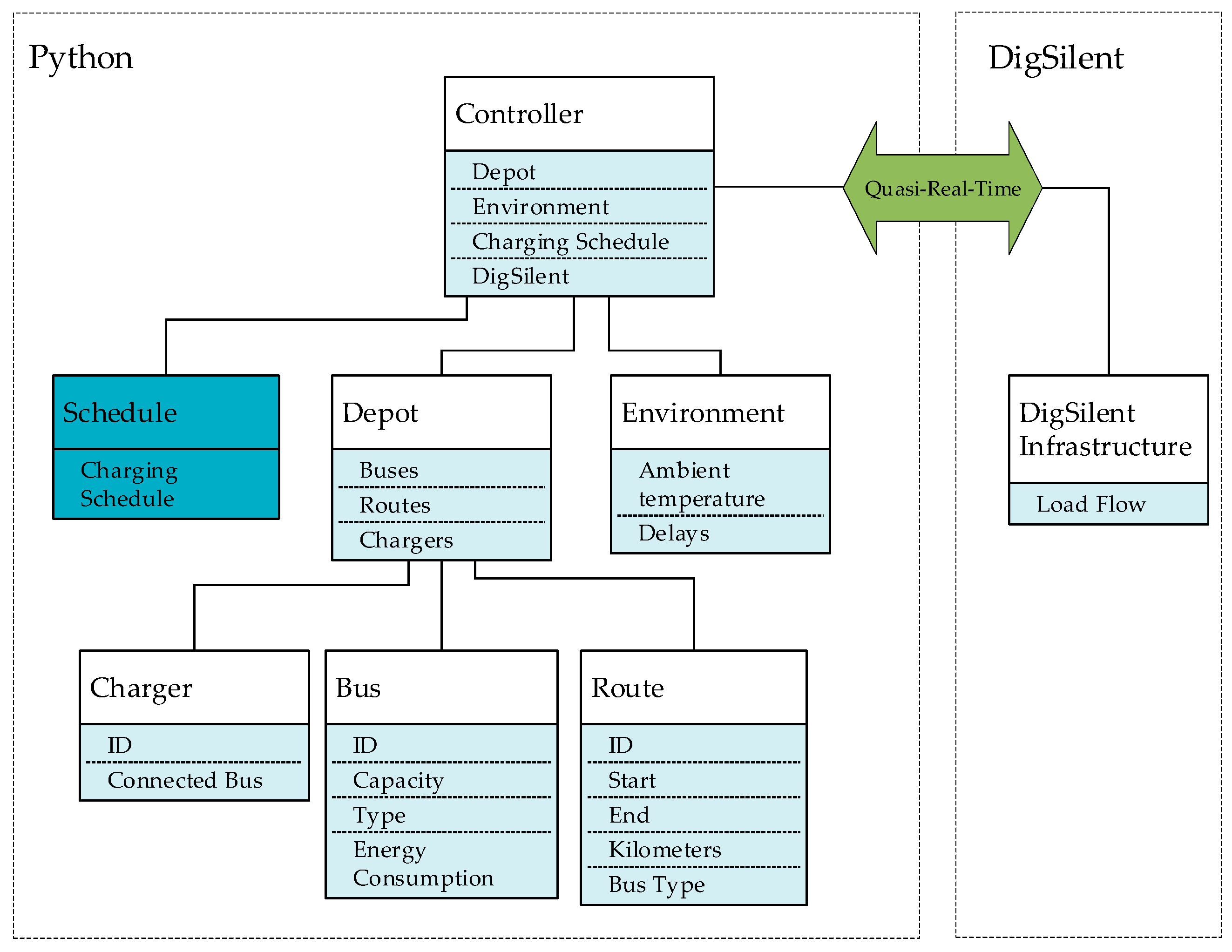
Bus Depot Simulator is a quasi-real-time cosimulation program based on software Python and DigSilent PowerFactory. It simulates the operation of a large-scale bus depot taking into consideration buses arriving and leaving, ambient temperature, delays due to traffic, dis/charging processes, etc. Figure 2 shows the structure of the program with the belonging classes.
The Controller manages the simulation by communicating with other classes such as Schedule, Depot and Environment, which are implemented in Python. The Controller also communicates with PowerFactory. The simulation runs in discrete time steps of one minute. For each minute, Python sends active power set points to PowerFactory based on the information, which buses are currently charging at which charging station. PowerFactory executes a Load Flow and sends the results back to Python. In that way, the user can follow the load profile of the depot in a quasi-real-time. During the initialization process, the Simulator creates all objects, establishes a connection with PowerFactory and loads the Schedule class. If there is no charging schedule in the Schedule class, the Simulator will charge the buses on demand as soon as they arrive to the depot. When a charging schedule is provided, the buses will charge only in the time interval defined in the schedule. In this way, the Simulator is independent from the Schedule class and can be used to validate any type of scheduling algorithms.
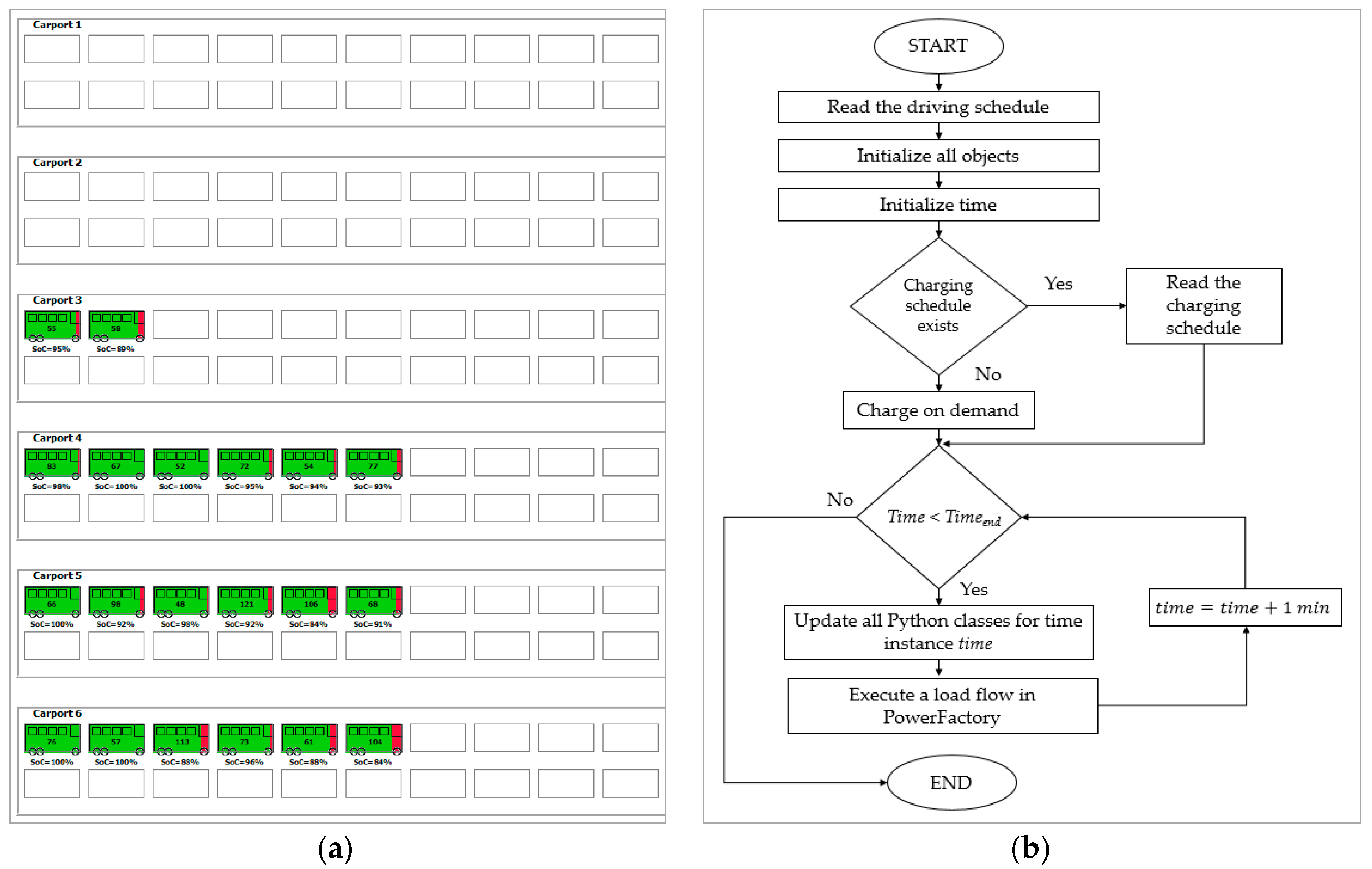
Figure 3 shows one part of the Bus Depot Simulator and the tab “Inside Depot”. This tab gives an overview of the buses currently at the depot together with their SoC. The figure also shows the flowchart with the co-simulation procedure.
Besides the tab “Inside Depot”, the Simulator also provides a deeper overview of different components of the system during the simulation, showing the following:
- The decisions the Controller is making.
- An overview of the buses currently driving outside of the depot (the route they are driving and the expected arrival back at the depot).
- Load profile at different terminals within the depot (active and reactive power at the connection point as well as on all carport terminals).
4. Methodology and the Proposed Algorithms
4.1. Methodology
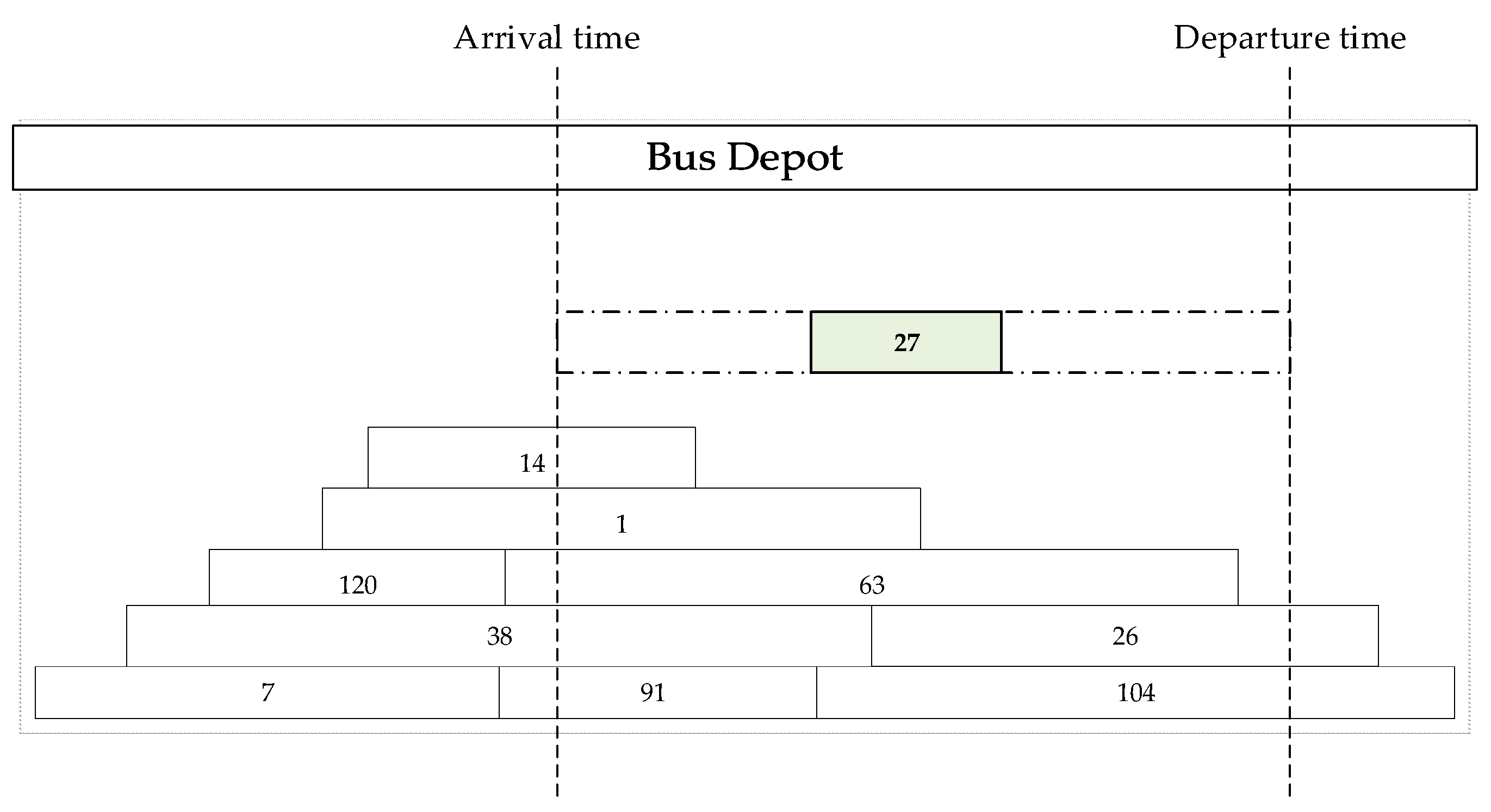
There are two perspectives to scheduling with electrical buses that can be observed independent or in correlation with each other; routes scheduling (which bus takes which route) and charging schedule (when and how much do the buses charge). This paper focuses on charging schedule, considering the routes are fixed as already discussed in Section 2.3. Each bus therefore has an already defined arrival and departure time. The time in between can be used for charging. Figure 4 gives a graphical representation of the mentioned timeline. The blocks represent the buses. Each bus draws power from the grid for two different tasks, charging, and preconditioning. Accordingly, there are two types of blocks, charging and preconditioning blocks. They can overlap or occur in different time slots. The length of the block is the time needed for preconditioning/charging. The height of the block is the power demand of the bus normalized based on the maximum charging power of 150 kW. There are three possible heights:
- Block height is 1: Bus is charging with 150 kW and there is no preconditioning.
- Block height is 0.567: Preconditioning is active and bus is charging with 85 kW.
- Block height is 0.433: Bus is not charging but there is preconditioning with 65 kW.
Preconditioning blocks are fixed in time and cannot be moved. Charging blocks can be freely moved in the time window between the arrival and departure time.
A certain number of buses in Figure 4 already arrived at the depot and started charging (white blocks in the figure). The number of buses charging simultaneously directly corresponds to the load at the depot. The problem is defined as follows; Where exactly between its arrival and departure time should the new coming bus 27 (green block in the figure) charge in order to minimize the number of buses charging simultaneously?
By observing the bus charging as a non-preemptive task, it is easy to reduce the above mentioned problem to a classical job scheduling problem. Two very similar variations of this problem have already been analyzed:
- Scheduling with release time and deadlines on a minimum number of machines.
- Scheduling non-preemptive jobs to minimize the peak demand.
Cieliebak et al. propose several exact and approximation algorithms for solving the problem of scheduling with release time and deadlines on a minimum number of machines [25]. Although this is a very similar problem to the bus depot, there is one fundamental difference. The jobs in the bus depot problem have three possible heights and Cieliebak et al. schedule jobs with the same height. Yaw et al. propose an exact algorithm, an approximation and a simple heuristic for the problem of scheduling non-preemptive jobs to minimize the peak demand in a smart grid [26]. They are scheduling jobs such as household appliances (dishwasher or water heater). These jobs have different heights, which makes it similar to the depot problem. However, this study focuses on non-resizable jobs. Using the example from Figure 4, this would mean that the blocks have fixed lengths. On the other hand, in the bus depot problem, the bus charging is considered a resizable job. The charging job resizing occurs due to preconditioning as shown in Figure 5. Bus 27 arrived to the depot at 23:00 in the evening and leaves again at 06:00 the following morning. It needs to charge for 1 h and 50 min with the maximum power of 150 kW. The bus is also preconditioning from 05:00 to 06:00 in the morning, before its departure. Shifting the charging of this bus to the morning hours, when it possibly overlaps with the preconditioning, will extend the time necessary to charge. This is due to the reduced charging power to the maximum of 85 kW.
The algorithms proposed by Yaw et al. are, to some extent, applicable to the bus depot problem but need to be adjusted.
4.2. Problem Definition
The problem of bus charging scheduling is defined similar to the job scheduling problems presented by Cieliebak et al. and Yaw et al. The bus b has an arrival time , departure time , charging start , charging length , and a height . The bus can charge in the interval [] with the following condition.
The difference is defined as the shifting time . If the difference equals to the length of the charging time , the shifting time is zero. In that case, there is only one possible charging interval for the bus. If on the other hand, there are multiple possible charging intervals for the bus. Charging interval is defined as so that
All possible charging intervals of bus b are defined with tuple so that
When calculating the intervals from the tuple it is necessary to calculate the length lb for each possible interval, since this length can change due to preconditioning.
The total height H at the time instance t is the sum of all heights of buses charging at that time:
The peak demand is the biggest height Hmax occurring during the complete analyzed period [0,T]. The goal is to minimize the Hmax by assigning one charging interval to each bus from its tuple of all possible charging intervals .
4.3. Greedy Algorithm
This algorithm uses a simple greedy logic. It defines a limit for the maximum allowed height . The algorithm chooses the charging intervals for each bus, so that the .The limit is reduced iteratively as long as it is possible to schedule all charging jobs. The smallest limit for which the algorithm manages to schedule all jobs is considered the minimum peak demand. Before executing the algorithm, the following steps are required.
- Step 1:
- Schedule all preconditioning jobs (these jobs are fixed and cannot be rescheduled).
- Step 2:
- Calculate all possible charging intervals for all buses and write them into tuples .
- Step 3:
- Organize all buses ascending by the arrival time.
- Step 4:
- Initialize the limit , where c is a curtailment factor.
The curtailment factor c depends on the number of buses at the depot. Haffner et al. did a sensitivity analysis and calculated the curtailment factor for different number of buses per module for the analyzed depot Alsterdorf [27]. They allowed the buses to charge on demand, without any charging schedule. The curtailment factor c is a limit for the number of buses that can charge simultaneously without affecting the charging process itself. The study showed that for 127 buses at the depot, the curtailment factor is 54%. is therefore initialized with c = 0.54.
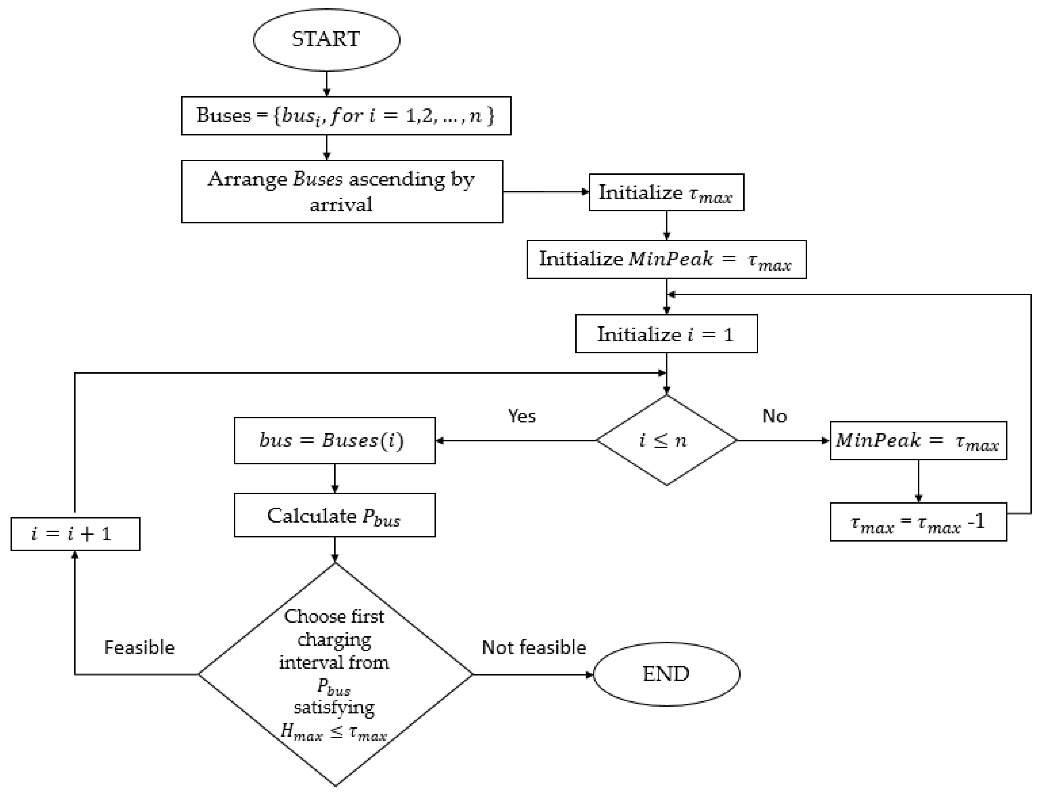
Figure 6 shows the flowchart of the proposed algorithm for a scenario of n buses. The variable MinPeak represents the minimum peak demand.
Organizing the buses ascending by the arrival time is an important step for this algorithm. It allows the buses to charge as soon as possible, usually at the far left side of the available interval [].
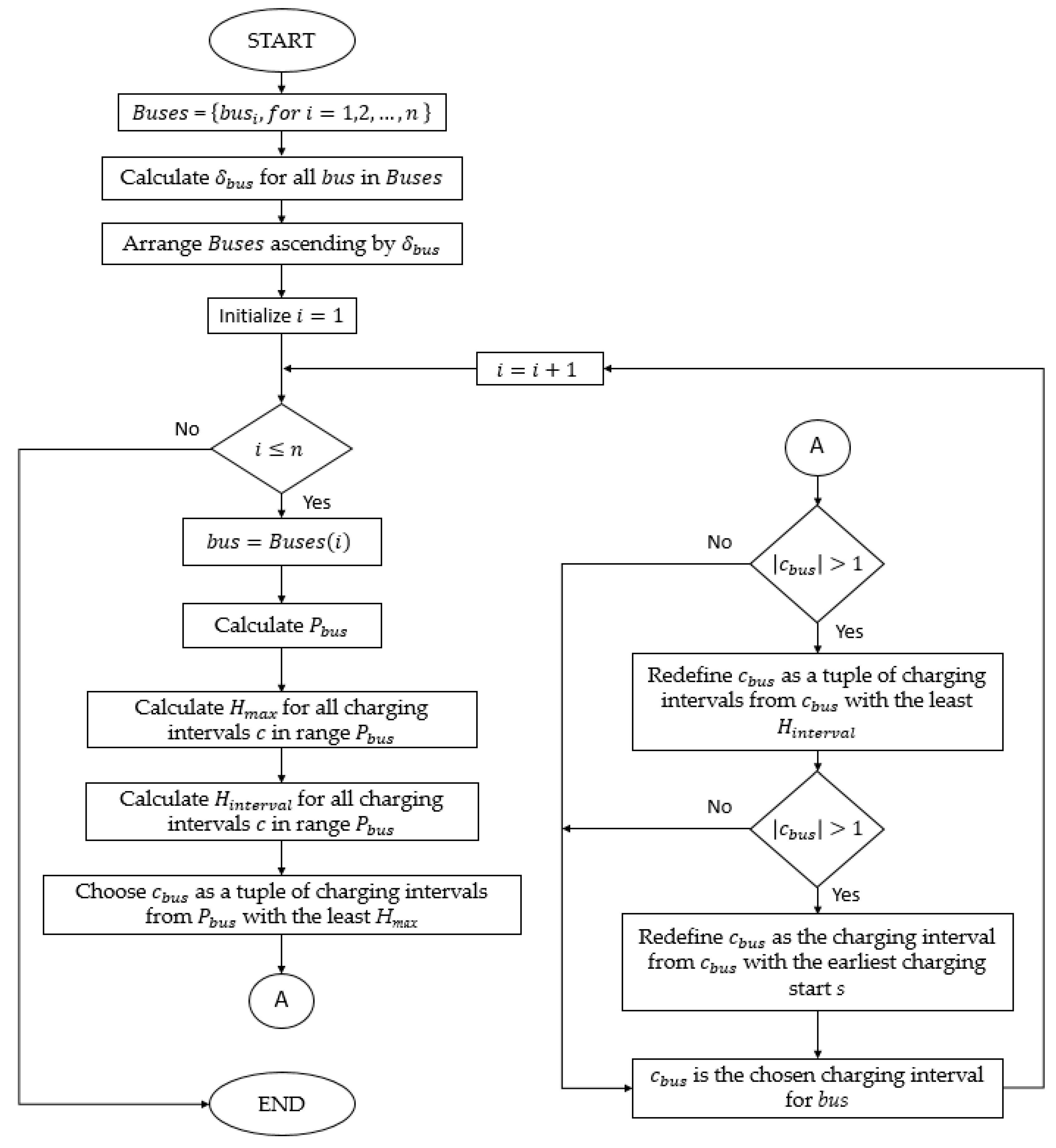
4.4. Heuristic Algorithm
This algorithm is an adjustment of the heuristic proposed by Yaw et al. An additional variable Hinterval is defined as the sum of all heights in one charging interval :
Before executing the algorithm, the following steps are necessary.
- Step 1:
- Schedule all preconditioning jobs (these jobs are fixed and cannot be rescheduled).
- Step 2:
- Calculate all possible charging intervals for all buses and write them into tuples .
- Step 3:
- Organize all buses ascending by their shifting time .
The algorithm flowchart for a scenario of n buses is presented in Figure 7. The greatest Hmax resulting from the presented logic is the minimum peak demand.
A crucial difference compared with the greedy algorithm is the preparation Step 3, organizing the buses ascending by their shifting time . The algorithm will first schedule the buses with no These jobs are fixed in time and cannot be shifted. In this way, the algorithm leaves the jobs, which are more flexible for later scheduling. The buses with big are scheduled last. Because of their flexibility, there is a high probability of scheduling without further increasing the height Hmax.
5. Results
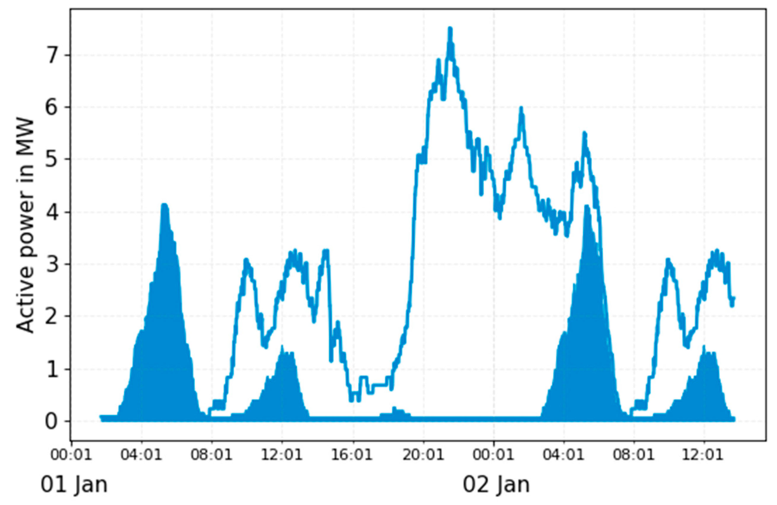
The two algorithms described in Section 4 were used to create charging schedules for the Bus Depot Simulator. The schedules were created for five working days but only a 36 h period was simulated. This is because there is no difference between the load profiles on different working days. The algorithms were observed in two separate scenarios. An additional third scenario, with no charging schedule was also observed. This scenario will further be referred to as the “original schedule”. Figure 8 shows the total load profile at the point of connection using the original schedule. The dark blue area shows the load resulting only from preconditioning. In this scenario, the buses are charged on demand as soon as they arrive to the depot. This leads to a high load at approximately 21:00 in the evening. The peak load in this case is 7.5 MW. The preconditioning has its peak at approximately 05:00 in the morning, with up to 4.1 MW. The preconditioning load cannot be rescheduled and it is considered to be the base load.
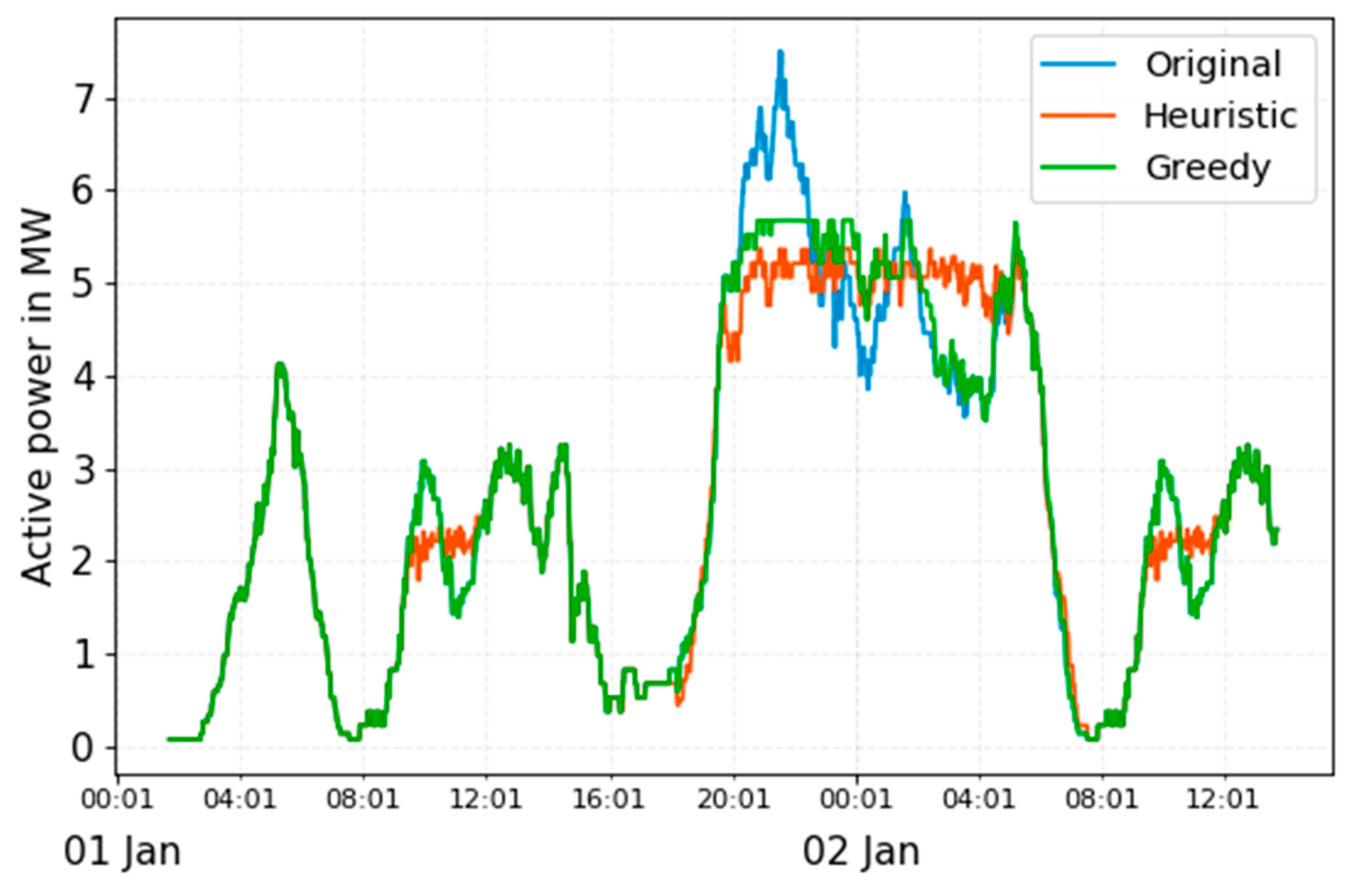
Figure 9 shows the load profiles resulting from the schedules created with the greedy and heuristic algorithm, compared to the original schedule. Greedy algorithm leads to a load peak of 5.67 MW, which corresponds to the maximum of 37 buses charging simultaneously. Heuristic schedule results in a peak load of 5.47 MW, corresponding to 35 buses charging in the same time. Compared to the original schedule, the load peak resulting from the greedy algorithm is 24.4% smaller and the load peak from the heuristic algorithm 27.1%. The heuristic schedule also shows deviation from the original schedule during the morning hours, between 9:00 and 12:00. Greedy algorithm did not reschedule any charging tasks in this period and shows no deviation from the original.
The load profile from the heuristic algorithm shows more small amplitude fluctuations during the night but it is generally better distributed. The greedy schedule resulted in a load profile, which was closer to constant in the time period from 20:00 to 23:00, but then showed a significant load dip at approximately 04:00.
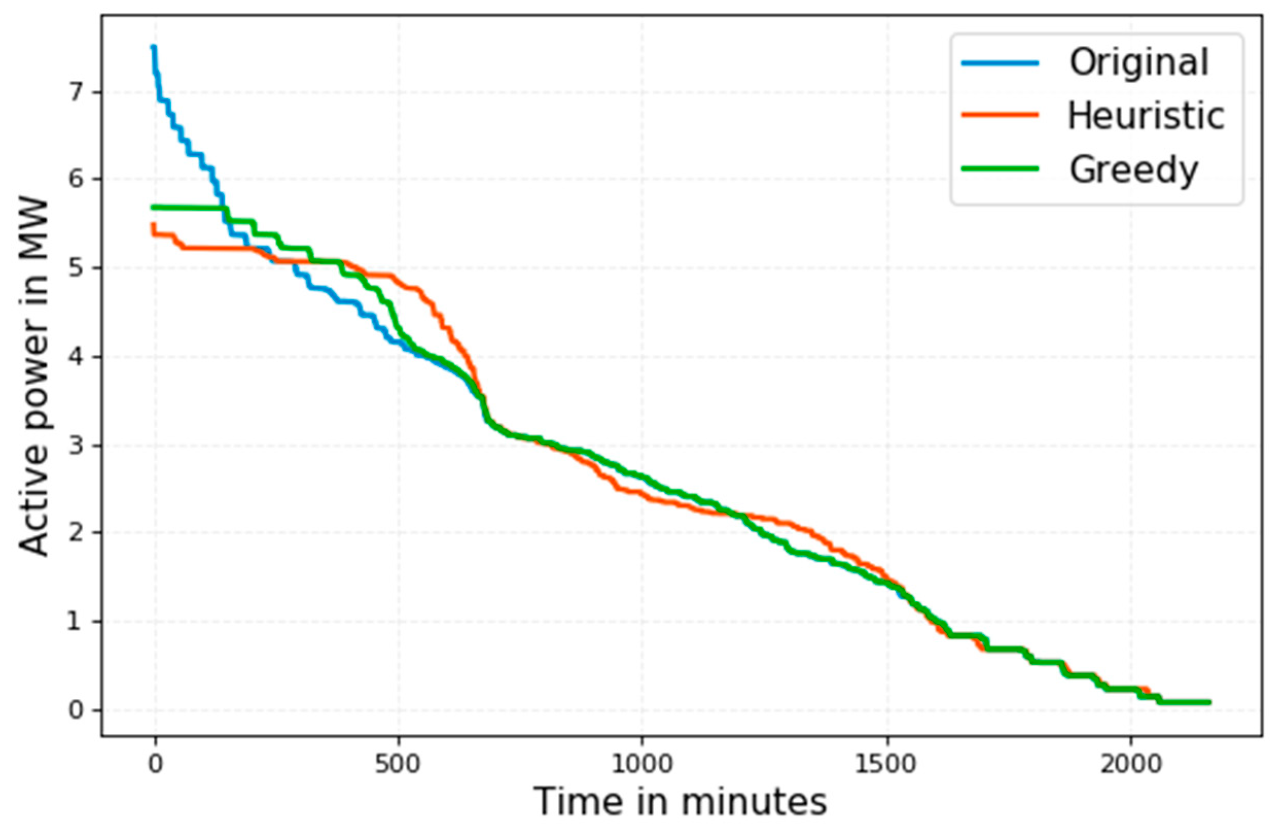
The difference in load distribution between the three compared scenarios is shown in Figure 10. The greedy algorithm minimized the peak demand but in the area of lower load it does not show any difference to the original schedule. Heuristic algorithm instead managed not only to reduce the peak demand but also to flatten the average load. The flattening occurred two times, once in the range from 5.0 to 5.47 MW, and once more in the range of 2.0 to 2.3 MW.
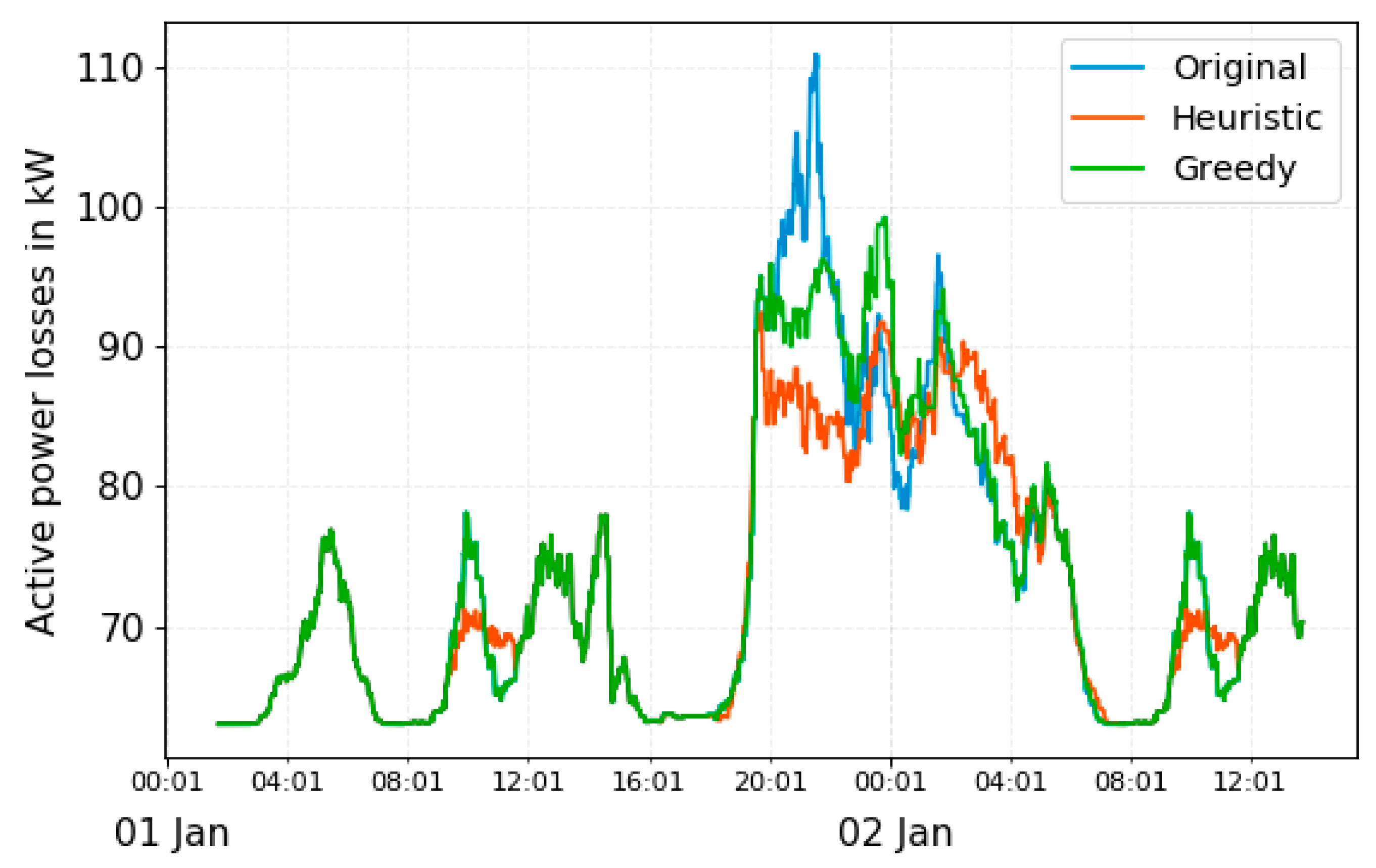
The active power losses in the transformers and cables within the bus depot for the three compared algorithms are shown in Figure 11. The original schedule resulted in energy losses of 2634 kWh for the analyzed period of 36 h. The greedy schedule leads to energy losses of 2636 kWh and the heuristic algorithm to 2611 kWh. Although the greedy schedule shows smaller load peak compared to the original, it resulted in slightly bigger energy losses with the increase of 2 kWh. The heuristic algorithm on the other hand shows smaller load peak and smaller energy losses. Compared to the original schedule, it reduced the energy losses for 23 kWh.
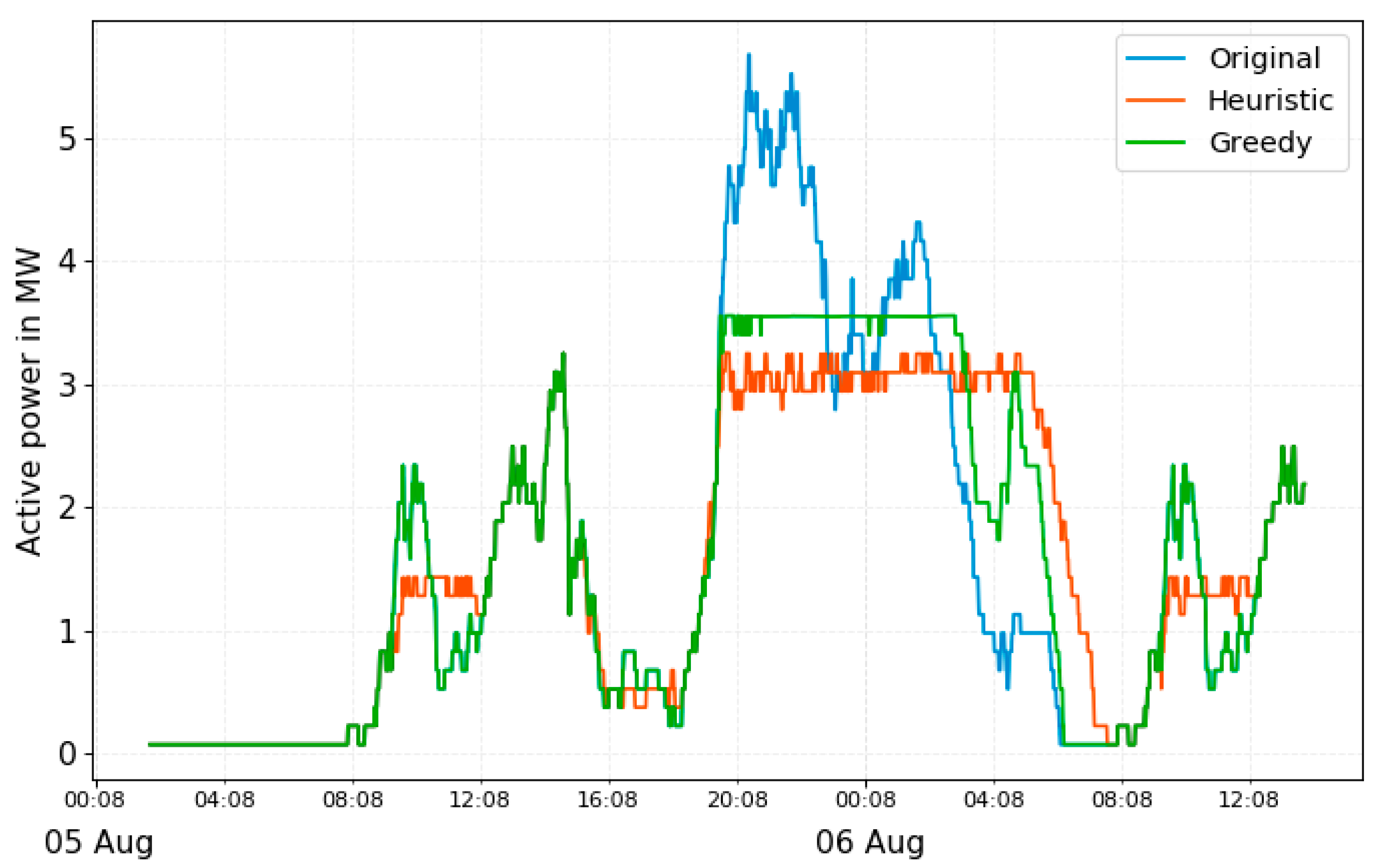
The preconditioning in winter months leads to a high load peak at the depot. However, during summer months, when there is no (or less) preconditioning, the peak load can be further reduced. Figure 12 shows the load profile from the original, heuristic and greedy schedule in summer months, assuming there is no preconditioning and the ambient temperature is 28 °C. The energy consumption of buses is smaller in the summer months. Therefore, the load profile resulting from the original schedule is also smaller than the one in winter and leads to a load peak of 5.7 MW. The greedy algorithm results in a load peak of 3.55 MW, corresponding to 23 buses charging in the same time. On the other hand, the heuristic algorithm shows better results and leads to a load peak of 3.27 MW and 21 buses charging simultaneously. Compared to the original schedule in this scenario, the greedy algorithm managed to reduce the load peak for 37.7% and the heuristic algorithm for 42.6%.
6. Discussion
This paper analyzes the charging scheduling problem on large-scale electric bus depots and proposes two algorithms for the load peak minimization. Real data from the bus depot in Alsterdorf in Hamburg were used for the simulation. The proposed algorithms were able to reduce the peak demand and flatten the peak load at the bus depot. Greedy schedule resulted in a slightly higher peak demand but an evenly distributed load during very high load periods. It managed to reduce the load peak for 24.4% compared to the original load profile. Nevertheless, it did not manage to reduce the cumulative energy losses within the depot. For the analyzed period of 36 h, it resulted in 2 kWh additional losses compared to the original load profile. Heuristic schedule in this case achieved an even smaller peak load and reduced it for 27.1% compared to the original load peak. It also reduced the energy losses for 23 kWh. The heuristic algorithm managed to distribute the average load better during the night as well as during the day, in the time from 09:00 to 12:00. However, it resulted in a load profile with more small amplitude fluctuations compared to greedy.
For the summer scenario, all algorithms showed smaller load peaks. This is due to the lower demand for preconditioning compared to the winter months. Greedy schedule managed to reduce the peak load for 37.7% compared to the original load profile. Heuristic schedule on the other hand reduced the load peak for 42.6%. In this case, the greedy algorithm resulted in a relatively flat load profile in time from 20:00 to 02:00. In the same time, the heuristic load profile once again showed many small amplitude load changes.
The charging process was considered as a non-preemptive job for the purposes of this paper. This means that once a bus has started charging, it continues until it reaches its goal SoC. The process can also be observed in a preemptive manner, allowing the bus to charge several times within its available charging interval. Additional interesting variable that could be included in the scheduling algorithms is the load forecast from the grid operator. The load profile at the bus depot would in that case support the overall load profile in the grid. Such scenarios, including online scheduling, are the topic of our future research.
Author Contributions
A.J. wrote the article and programmed the proposed algorithms. A.J. and M.E. developed the proposed algorithms. D.S. supervised the work and provided helpful feedback regarding both the algorithms and the article.
Funding
This work is a part of the project Accompanying Research for Charging Infrastructure on Bus Depots. It is supported by the German Federal Ministry of Transport and Digital Infrastructure (AKZ G20/3552.1/3).
Acknowledgments
The authors would like to thank HOCHBAHN AG for the good cooperation and the provided data.
Conflicts of Interest
The authors declare no conflict of interest.
References
- Alonso, M.; Amaris, H.; Germain, J.G.; Galan, J.M. Optimal Charging Scheduling of Electric Vehicles in Smart Grids by Heuristic Algorithms. Energies 2014, 7, 2449–2475. [Google Scholar] [CrossRef] [Green Version]
- Hu, J.; Morais, H.; Sousa, T.; Lind, M. Electric vehicle fleet management in smart grids: A review of services, optimization and control aspects. Renew. Sustain. Energy Rev. 2016, 56, 1207–1226. [Google Scholar] [CrossRef] [Green Version]
- Yang, Y.; Zhang, W.; Niu, L.; Jiang, J. Coordinated Charging Strategy for Electric Taxis in Temporal and Spatial Scale. Energies 2015, 8, 1256–1272. [Google Scholar] [CrossRef] [Green Version]
- Abul’Wafa, A.; El’Garably, A.; Mohamed, W. Uncoordinated vs Coordinated Charging of Electric Vehicles in Distribution System Performance. Int. J. Eng. Inf. Syst. 2017, 1, 54–65. [Google Scholar]
- Ma, Z.; Callaway, D.S.; Hiskens, I.A. Decentralized Charging Control of Large Populations of Plug-in Electric Vehicles. IEEE Trans. Control Syst. Technol. 2013, 21, 67–68. [Google Scholar] [CrossRef]
- Deb, S.; Tammi, K.; Kalita, K.; Mahanta, P. Impact of Electric Vehicle Charging Station Load on Distribution Network. Energies 2018, 11, 178. [Google Scholar] [CrossRef]
- Mohamed, M.; Farag, H.; El-Taweel, N.; Ferguson, M. Simulation of electric buses on a full transit network: Operational feasibility and grid impact analysis. Electr. Power Syst. Res. 2017, 142, 163–175. [Google Scholar] [CrossRef]
- Thiringer, T.; Haghbin, S. Power Quality Issues of a Battery Fast Charging Station for a Fully-Electric Public Transport System in Gothenburg City. Batteries 2015, 1, 22–33. [Google Scholar] [CrossRef] [Green Version]
- Schumann, M.; Meyer, M.; Dietmannsberger, M.; Detlef, S. Demands on the Electrical Grid due to Electromobility in Hamburg. In Proceedings of the 1st E-Mobility Power System Integration Symposium, Berlin, Germany, 23 October 2017. [Google Scholar]
- Chao, Z.; Chen, X. Optimizing Battery Electric Bus Transit Vehicle Scheduling with Battery Exchanging: Model and Case Study. Procedia Soc. Behav. Sci. 2013, 96, 2725–2736. [Google Scholar] [CrossRef] [Green Version]
- Dai, Q.; Cai, T.; Duan, S.; Zhang, W.; Zhao, J. A smart energy management system for electric city bus battery swap station. In Proceedings of the IEEE Conference and Expo Transportation Electrification Asia-Pacific (ITEC Asia-Pacific), Beijing, China, 31 August–3 September 2014. [Google Scholar]
- You, P.; Yang, Z.; Zhang, Y.; Low, S.H.; Sun, Y. Optimal Charging Schedule for a Battery Switching Station Serving Electric Buses. IEEE Trans. Power Syst. 2016, 31, 3473–3483. [Google Scholar] [CrossRef]
- Zhou, D.; Ren, Z.; Sun, K.; Dai, H. Optimization Method of Fast Charging Buses Charging Strategy for Complex Operating Environment. In Proceedings of the 2nd IEEE Conference on Energy Internet and Energy System Integration (EI2), Beijing, China, 20–22 October 2018. [Google Scholar]
- Yan, Y.; Jiang, J.; Zhang, W.; Huang, M.; Chen, Q.; Wang, H. Research on Power Demand Suppression Based on Charging Optimization and BESS Configuration for Fast-Charging Stations in Beijing. Appl. Sci. 2018, 8, 1212. [Google Scholar] [CrossRef]
- Yang, C.; Lou, W.; Yao, J.; Xie, S. On Charging Scheduling Optimization for a Wirelessly Charged Electric Bus System. IEEE Trans. Intell. Transp. Syst. 2018, 19, 1814–1826. [Google Scholar] [CrossRef]
- Paul, T.; Yamada, H. Operation and charging scheduling of electric buses in a city bus route network. In Proceedings of the 17th IEEE International Conference on Intelligent Transportation Systems (ITSC), Qingdao, China, 8–11 October 2014. [Google Scholar]
- Leou, R.C.; Hung, J.J. Optimal Charging Schedule Planning and Economic Analysis for Electric Bus Charging Stations. Energies 2017, 10, 483. [Google Scholar] [CrossRef]
- Gao, Y.; Guo, S.; Ren, J.; Zhao, Z.; Ehsan, A.; Zheng, Y. An Electrical Bus Power Consumption Model and Optimization of Charging Scheduling Concerning Multi-External Factors. Energies 2018, 11, 2060. [Google Scholar] [CrossRef]
- Rinaldi, M.; Parisi, F.; Laskaris, G.; D’Adriano, A.; Viti, F. Optimal dispatching of electric and hybrid buses subject to scheduling and charging constraints. In Proceedings of the 21st International Conference on Intelligent Transportation Systems (ITSC), Maui, HI, USA, 4–7 November 2018. [Google Scholar]
- Houbbadi, A.; Trigui, R.; Pelissier, S.; Bouton, T.; Redondo-Iglesias, E. Multi-Objective Optimisation of the Management of Electric Bus Fleet Charging. In Proceedings of the IEEE Vehicle Power and Propulsion Conference (VPPC), Belfort, France, 11–14 December 2017. [Google Scholar]
- Jiang, M.; Zhang, Y.; Zhang, Y.; Zhang, C.; Zhang, K.; Zhang, G.; Zhao, Z. Operation and Scheduling of Pure Electric Buses under Regular Charging Mode. In Proceedings of the 21st International Conference on Intelligent Transportation Systems (ITSC), Maui, HI, USA, 4–7 November 2018. [Google Scholar]
- Wang, G.; Xie, X.; Zhang, F.; Liu, Y.; Zhang, D. bCharge: Data-Driven Real-Time Charging Scheduling for Large-Scale Electric Bus Fleets. In Proceedings of the IEEE Real-Time Systems Symposium (RTSS), Nashville, TN, USA, 11–14 December 2018. [Google Scholar]
- Chen, H.; Hu, Z.; Xu, Z.; Li, J.; Zhang, H.; Xia, X.; Ning, K.; Peng, M. Coordinated charging strategies for electric bus fast charging stations. In Proceedings of the IEEE PES Asia-Pacific Power and Energy Engineering Conference (APPEEC), Xi’an, China, 25–28 October 2016. [Google Scholar]
- Dietmannsberger, M.; Schumann, M.; Meyer, M.; Schulz, D. Modelling the Electrification of Bus Depots using Real Data: Consequences for the Distribution Grid and Operational Requirements. In Proceedings of the 1st E-Mobility Power System Integration Symposium, Berlin, Germany, 23 October 2017. [Google Scholar]
- Cieliebak, M.; Erlebach, T.; Hennecke, F.; Weber, B.; Widmayer, P. Scheduling with Release Times and Deadlines on a Minimum Number of Machines. In Exploring New Frontiers of Theoretical Informatics; Levy, J.J., Mayr, E.W., Mitchell, J.C., Eds.; Springer: Boston, MA, USA, 2004; Volume 155, pp. 209–222. [Google Scholar]
- Yaw, S.; Mumey, B. Scheduling Non-Preemptible Jobs to Minimize Peak Demand. Algorithms 2017, 10, 122. [Google Scholar] [CrossRef]
- Haffner, L.; Schumann, M.; Schulz, D.; Dietmannsberger, M. Evaluation of Modular Infrastructure Concepts for Large-Scaled Electric Bus Depots. In Proceedings of the 2nd E-Mobility Power System Integration Symposium, Stockholm, Sweden, 31 August 2018. [Google Scholar]
Figure 1.
Electrical infrastructure on the Bus Depot Alsterdorf with the detailed representation of the Carport No. 6.
Figure 1.
Electrical infrastructure on the Bus Depot Alsterdorf with the detailed representation of the Carport No. 6.

Figure 2.
Cosimulation process with Python and Power Factory.

Figure 3.
(a) Bus Depot Simulator user interface with the tab “Inside Depot”, showing the buses currently at the depot and their SoC and (b) the cosimulation procedure presented with a flowchart.
Figure 3.
(a) Bus Depot Simulator user interface with the tab “Inside Depot”, showing the buses currently at the depot and their SoC and (b) the cosimulation procedure presented with a flowchart.

Figure 4.
Graphical representation of the scheduling problem with several random buses already charging (white blocks) and a new bus arriving at the depot (green block).
Figure 4.
Graphical representation of the scheduling problem with several random buses already charging (white blocks) and a new bus arriving at the depot (green block).

Figure 5.
Change in the length of the charging block (green) due to the preconditioning block (blue) for two different scenarios: (a) no overlapping with preconditioning; charging time is 1 h and 50 min and (b) overlapping with preconditioning for 15 min; charging time is 2 h and 2 min.
Figure 5.
Change in the length of the charging block (green) due to the preconditioning block (blue) for two different scenarios: (a) no overlapping with preconditioning; charging time is 1 h and 50 min and (b) overlapping with preconditioning for 15 min; charging time is 2 h and 2 min.

Figure 6.
Greedy algorithm presented with a flowchart.

Figure 7.
Flowchart representing the heuristic algorithm.

Figure 8.
Load profile resulting from the original charging schedule together with the preconditioning load.
Figure 8.
Load profile resulting from the original charging schedule together with the preconditioning load.

Figure 9.
Load profiles resulting from the original, greedy, and heuristic schedule.

Figure 10.
Load distribution from the three compared algorithms during the simulated time.

Figure 11.
Losses in transformers and cables resulting from the original, greedy and heuristic schedule.
Figure 11.
Losses in transformers and cables resulting from the original, greedy and heuristic schedule.

Figure 12.
Load profile resulting from the original, heuristic and greedy schedule in the summer months, with no preconditioning and the ambient temperature of 28 °C.
Figure 12.
Load profile resulting from the original, heuristic and greedy schedule in the summer months, with no preconditioning and the ambient temperature of 28 °C.


Table 1.
Energy consumption of electric buses in dependence on the ambient temperature.
| Bus Type | −15 °C | +20 °C | +28 °C | Unit |
|---|---|---|---|---|
| Standard | 2.11 | 1.40 | 1.60 | kWh/km |
| Articulated | 3.25 | 2.05 | 2.40 | kWh/km |
| Double articulated | 4.50 | 2.68 | 3.17 | kWh/km |
Table 2.
Example of an assembled driving schedule for buses at the bus depot Alsterdorf.
| Bus ID | Route ID | Departure Time | Arrival Time | SoC Before Trip | SoC After Trip |
|---|---|---|---|---|---|
| 1 | 66,001 | 05:43 | 09:51 | 100% | 80% |
| 2 | 66,002 | 06:04 | 14:50 | 100% | 50% |
| 3 | 66,003 | 07:07 | 13:15 | 100% | 60% |
© 2019 by the authors. Licensee MDPI, Basel, Switzerland. This article is an open access article distributed under the terms and conditions of the Creative Commons Attribution (CC BY) license (http://creativecommons.org/licenses/by/4.0/).
Share and Cite
MDPI and ACS Style
Jahic, A.; Eskander, M.; Schulz, D. Charging Schedule for Load Peak Minimization on Large-Scale Electric Bus Depots. Appl. Sci. 2019, 9, 1748. https://doi.org/10.3390/app9091748
AMA Style
Jahic A, Eskander M, Schulz D. Charging Schedule for Load Peak Minimization on Large-Scale Electric Bus Depots. Applied Sciences. 2019; 9(9):1748. https://doi.org/10.3390/app9091748
Chicago/Turabian StyleJahic, Amra, Mina Eskander, and Detlef Schulz. 2019. "Charging Schedule for Load Peak Minimization on Large-Scale Electric Bus Depots" Applied Sciences 9, no. 9: 1748. https://doi.org/10.3390/app9091748
Note that from the first issue of 2016, this journal uses article numbers instead of page numbers. See further details here.