Surrogate Neural Network Model for Prediction of Load-Bearing Capacity of CFSS Members Considering Loading Eccentricity


Institute of Research and Development, Duy Tan University, Da Nang 550000, Vietnam
Appl. Sci. 2020, 10(10), 3452; https://doi.org/10.3390/app10103452
Submission received: 21 April 2020
/
Revised: 8 May 2020
/
Accepted: 13 May 2020
/
Published: 16 May 2020
(This article belongs to the Special Issue Advances on Structural Engineering)
Abstract
:In this study, a surrogate Machine Learning (ML)-based model was developed, to predict the load-bearing capacity (LBC) of concrete-filled steel square hollow section (CFSS) members, considering loading eccentricity. The proposed Artificial Neural Network (ANN) model was trained and validated against experimental data using the following error measurement criteria: coefficient of determination (R2), slope of regression, root mean square error (RMSE) and mean absolute error (MAE). A parametric study was conducted to calibrate the parameters of the ANN model, including the number of neurons, activation function, cost function and training algorithm, respectively. The results showed that the ANN model can provide reliable and effective prediction of LBC (R2 = 0.975, Slope = 0.975, RMSE = 294.424 kN and MAE = 191.878 kN). Sensitivity analysis showed that the geometric parameters of the steel tube (width and thickness) and the compressive strength of concrete were the most important variables. Finally, the effect of eccentric loading on the LBC of CFSS members is presented and discussed, showing that the ANN model can assist in the creation of continuous LBC maps, within the ranges of input variables adopted in this study.
1. Introduction
Composite materials are very widely employed in the construction industry, due to their efficient structural performance (high strength and ductility) and reasonable cost [1]. In this context, concrete-filled steel square hollow section (CFSS) members utilize the advantages of both steel and concrete. They comprise a steel hollow section of square shape, filled with plain concrete. On the one hand, they may be used as columns and beam-columns in high-rise buildings [2,3]. On the other hand, CFSS members could serve as beams in low-rise infrastructures (i.e., industrial buildings) [4]. Indeed, CFSS members have become increasingly popular in structural systems, due to their favorable structural performance characteristics, including high strength and ductility, and easy beam-to-column connection manufacturing process [5,6,7,8,9,10].
In terms of research and development, extensive investigations have been carried out on the complex problem of concrete-filled steel tubular members over the last fifty years. One of the first studies on the compressive behavior of CFSS was done in the 1970s by Tomii et al. [11], showing that the load-bearing capacity (LBC) of CFSS members depended heavily on various parameters: the width-to-thickness ratio of the steel tube, strength of the concrete core, etc. In the past few years, with the increase in high-rise construction, the study of CFSS members under compression has received growing amounts of attention from both engineers and scholars, including Aslani et al. [12], Chen et al. [13], Khan et al. [14], Xiong et al. [15], Du et al. [16], Lai and Ho [8] and Yan et al. [17]. These works revealed that CFSS members exhibited good strength, strong ductility and beneficial construction characteristics. Although there are usually members under eccentric loading in buildings (i.e., corner and side columns), there is a scant body of work examining the compressive behavior of eccentrically loaded CFSS columns [18,19]. Therefore, it is absolutely crucial to study this type of composite structures under eccentric loading, especially in predicting their LBC [20,21].
In recent decades, Machine Learning (ML) approaches have been extensively used for predicting the behavior of structural members [22,23,24]. Such models exhibit significant advantages cannot be found in traditional techniques (i.e., linear regression, regularization, response surface methodology and multiple regression [25,26,27]). The main reason for such superiority is that ML techniques do not require assumptions or predefined constraints about the form of the model (for instance between dependent and independent variables) [25,26,27,28]. Nonetheless, several investigations have been proposed to relate physical laws and ML techniques. For instance, Zhu et al. [29] discussed physics-constrained deep learning in a high-dimensional surrogate model. Stewart et al. [30] proposed label-free supervision for an Artificial Neural Network (ANN) model, under constraints derived from prior known laws of physics. Berg et al. [31] trained an ANN to approximate the solution by minimizing the violation of the governing Partial Differential Equations in complex geometries. Despite the lack of physical constraints in ML models (could be considered as their major limitation), they are more and more used as a surrogate model in various problems, especially for capturing and tracking nonlinear behavior between inputs and outputs [32,33,34]. Many researchers have studied the enhanced capability of the ANN and compared it with conventional models for various structural engineering applications, including Sarir et al. [22], Tran et al. [24] and Nadepour et al. [33]. The results of these studies showed that ML approaches outperformed the conventional models. The most common ML techniques used in civil engineering problems include Support-Vector Machine [35], Regression Tree [36], Random forest [37] and especially ANN [22,24,34,38,39,40].
The main objective of this work is to develop a surrogate ML-based model to predict the LBC of CFSS columns considering the effect of eccentric loading. To this end, an ANN was developed, because of its ability to deal with high-dimensional problems. The ANN model was optimized by performing a parametric study, involving the ANN’s architecture (i.e., number of hidden layers and number of neurons in hidden layers), activation function, cost function and training function. In order to train and validate the ANN model, a range of error measurement criteria were used: coefficient of determination (R2), slope of regression, Root Mean Squared Error (RMSE) and Mean Absolute Error (MAE). A sensitivity analysis was also performed, to highlight the influence of each input variable on the output response. In addition, an uncertainty analysis was applied to estimate the prediction confidence intervals. We expect to provide a reliable contribution to progress in the modeling and prediction of the compressive behavior of CFSS members.
2. Materials and Methods
2.1. Database
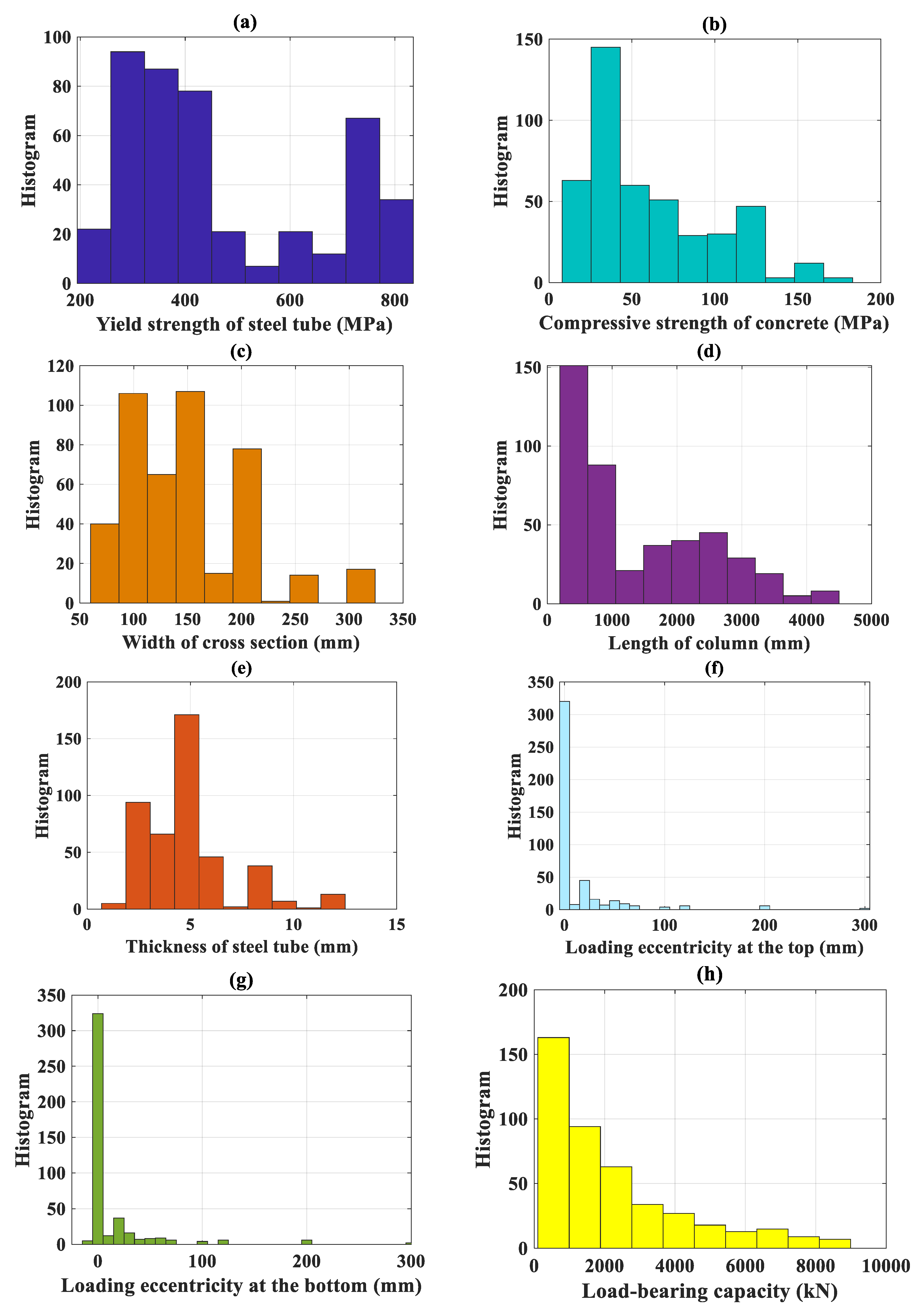
In the present paper, as the focus is on CFSS members under both concentric and eccentric loading, the input data including the mechanical properties of steel and concrete (yield strength and compressive strength, respectively), the cross-sectional width, column length, steel tube thickness, loading eccentricities at the top and bottom of the member, were collected from the available literature. A total of 443 tests on CFSS members under compression served as a database, involving 314 concentric and 129 eccentric cases, respectively [41,42,43]. Figure 1 presents a diagram of CFSS members under eccentric loading, together with their geometrical parameters. A primarily statistical analysis of the database is shown in Table 1, including the min, average, max, standard deviation (StD) and coefficient of variation (CV) of all variables. It is apparent that the yield strength of the steel tube varies from 194.18 MPa to 835 MPa, with a mean value of 472.79 MPa and StD of 192.91 MPa. The compressive strength of the concrete core ranges from 7.9 MPa to 183 MPa, with a mean value of 59.84 MPa and StD of 36.50 MPa. The width of the cross section varies from 60 mm to 324 mm, with a mean value of 147.18 mm and StD of 46.86 mm. The member’s length ranges from 195 mm to 4500 mm, with a mean value of 1426.55 mm and StD of 1110.43 mm. The thickness of the steel tube varies from 0.7 mm to 12.5 mm, with mean value of 4.88 mm and StD of 2.17 mm. The loading eccentricity at the top of the member ranges from 0 to 300 mm, with a mean value of 14.58 mm and StD of 37.10 mm. The loading eccentricity at the bottom of the member varies from −25 to 300 mm, with a mean value of 13.51 mm and StD of 37.02 mm. Figure 2 shows the corresponding histograms of variables in the database. It is seen that, for several ranges of values, not enough data have been collected to ensure a good homogeneity. Consequently, missing data should be completed in further researches. Finally, investigations dealing with problem of inhomogeneity in the data can be referred to Wang et al. [44], Busse and Buhmann [45], and Bühlmann and Meinshausen [46].
2.2. Methods Used
2.2.1. Artificial Neural Network
One of the most widely used methods in the field of data mining and Machine Learning is ANN, introduced in 1943 by McCulloch and Pitts [47]. This concept, inspired by the biological neural networks of human brains, is an inter-connected group of artificial nodes performing computational tasks [48]. Similar to a biological neuron composed of dendrites, a cell body, axon and synapse [34], an artificial neuron has inputs, variable weights and outputs [49]. Such an inter-connected system of nodes is able to understand and solve complex problems that exhibit a nonlinear relationship between causal factors and responses [50,51]. Indeed, the ANN model has relevant benefits not found in conventional computational models. Hypotheses or pre-constraints during modelling are not necessary when training the ANN model [28,52]. The technique is able to analyze and discover complex relationships and processes in the data [53,54]. From a computational point of view, ANN is very efficient for high-dimensional problems, because of its excellent capacity in parallel processing [55,56], however, it is still very limited to real-time and industrial applications [57,58]. Nonetheless, the performance of ANN is affected by other problems, including over-fitting [59], noisy data [60] and susceptibility to training data [61].
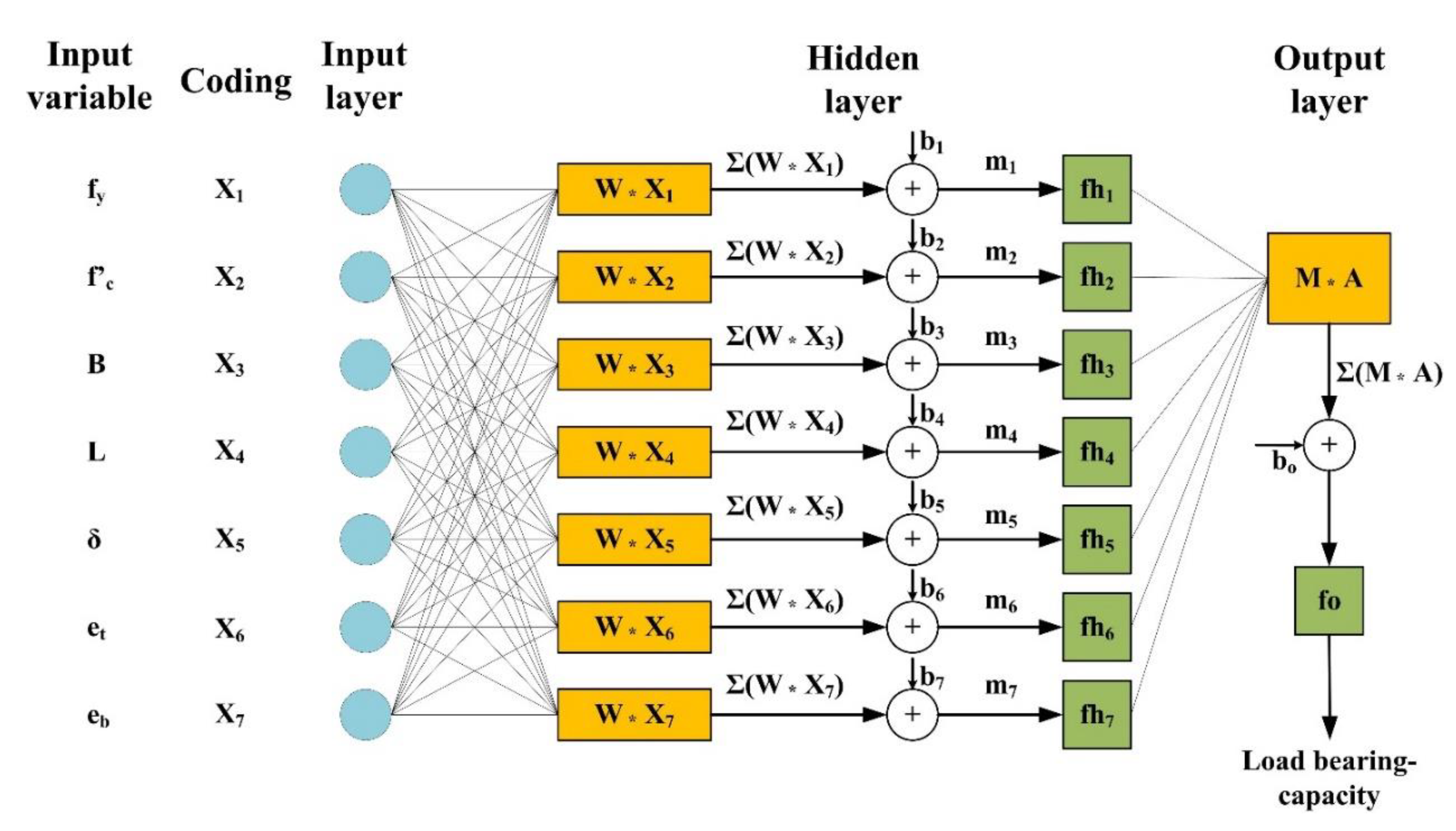
The structure of an ANN model comprises three types of layer: input (variables), hidden (functional layer), and output layers (network’s outcomes). These layers are connected by the artificial computational neurons, which compute the weighting parameters of the model. ANN can contain multiple hidden layers. For simplification purposes, the following description is presented for a single hidden-layer neural network. The following nonlinear function is generalized by the ANN model [62,63,64,65]:
where X is the input vector and Y is the predicted variable. The function f can be fully detailed as follows:
where W, fh and b are the weight matrix, activation function and bias vector of the hidden layer; while M, fo and bo are the weight matrix, activation function and bias vector of the output layer, respectively. Figure 3 introduces the architecture of the ANN model involving one hidden layer. The ANN model is trained (i.e., estimation of the weight matrix and bias vector) with an optimization method, using backpropapagation as a gradient computing technique [66,67]. More precisely, the optimizer allows locating the minimum of the cost function based on gradient descent, whereas the backpropagation allows computing such gradient that the optimizer uses.
For a given ML problem, it is very difficult to determine which activation function and training algorithm are appropriate. This depends on many factors, including the complexity of the problem, the number of data points in the training set, the number of weights and biases in the network and the error goal [68]. Therefore, in this study, a parametric study was conducted to select the most appropriate parameters for the problem at hand. According to various works (e.g., [22,34,38]), one hidden layer can solve any complex function in a network. Therefore, the number of hidden layers was fixed at 1 in this study. However, other parameters needing to be calibrated include the activation function, cost function, training function and the number of neurons in the hidden layer.
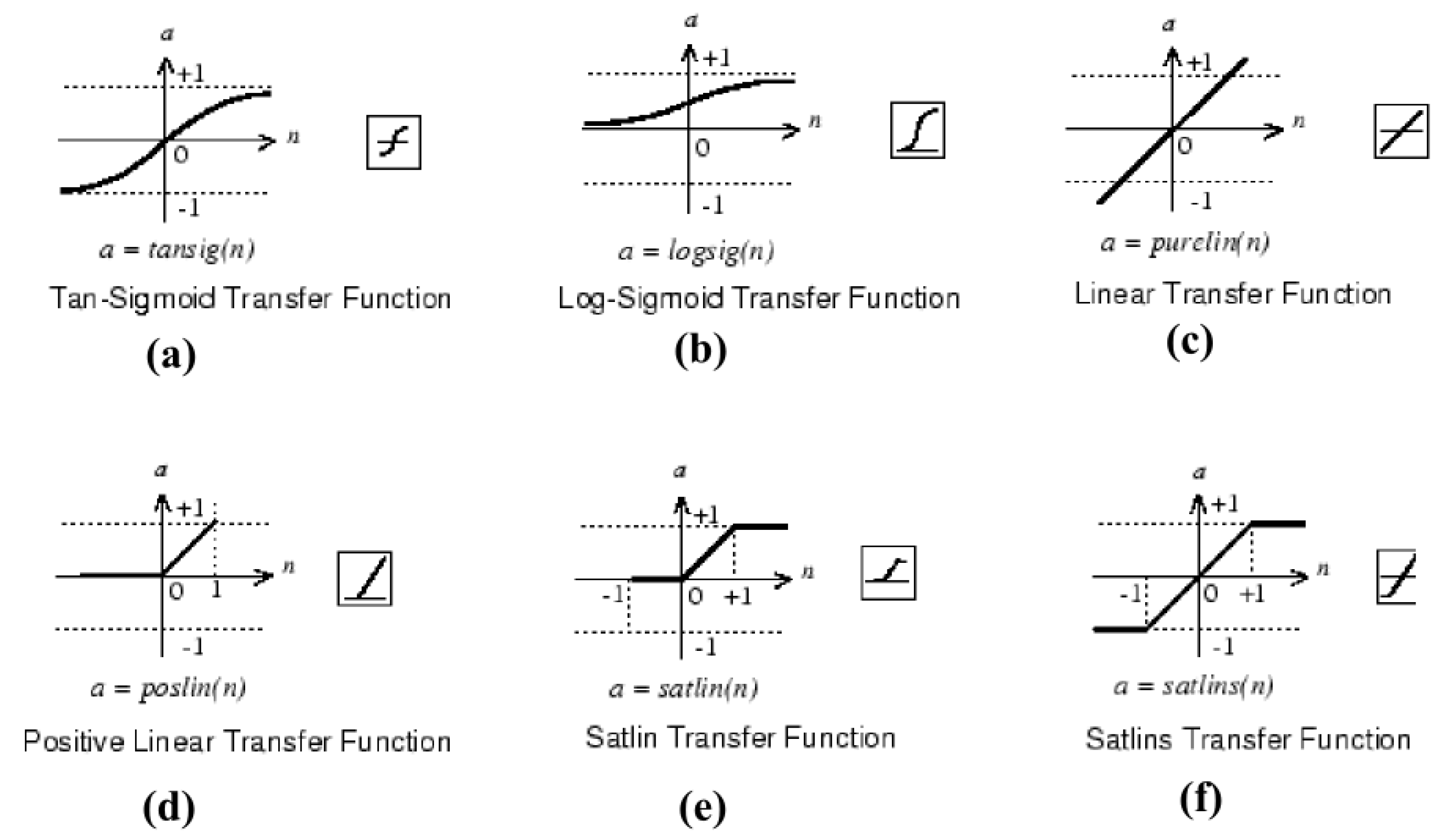
In any ML model, activation functions could affect: (i) the output response, (ii) the accuracy and (iii) the computational efficiency during the training process [69,70]. In this work, six activation functions were evaluated, as highlighted in Figure 4 [69,70,71,72]:
- Hyperbolic tangent sigmoid function, denoted by tansig;
- Log-sigmoid function, denoted by logsig;
- Linear function, denoted by purelin;
- Positive linear function, denoted by rectilin;
- Saturating linear function, denoted by satlin;
- Symmetric saturating linear function, denoted by satlins.
On the other hand, three cost functions during the process of optimizing the weight parameters of the ANN model were employed: mean squared error, sum absolute error and mean absolute error [73]. The number of neurons in the hidden layer varied from 1 to 30 [68]. Finally, eight backpropagation training algorithms were employed, as listed below:
- Levenberg-Marquardt [74], denoted by LM;
- Scaled conjugate gradient [75], denoted by SCG;
- BFGS quasi-Newton [76], denoted by BFG;
- Resilient [77], denoted by RP;
- Conjugate gradient with Powell-Beale restarts [78], denoted by CGB;
- Conjugate gradient with Fletcher-Reeves updates [79], denoted by CGF;
- Conjugate gradient with Polak-Ribiére updates [79], denoted by CGP;
- One-step secant [80], denoted by OSS.
2.2.2. Monte Carlo Random Sampling Technique
The main idea of the Monte Carlo method is that the output is computed by repeating random sampling of variables from the input space [81,82]. For this reason, the Monte Carlo method is widely applied: (i) in order to propagate the variability of inputs on the output response; and (ii) based on statistical analysis of output, several post-treatments such as robustness and/or sensitivity analyses can be thoroughly conducted [83,84,85]. Using a Monte Carlo simulation, the higher the number of runs, the higher the reliability of the response archived. For a random variable, if we have a sufficient number of independent realizations, its expected value is closely related to its mean value. Therefore, the convergence estimator for the mean value is unbiased, as demonstrated in the literature (e.g., [86,87]). In this study, a statistical estimator for the mean value was used to quantify the convergence of a given variable K. For the mean value, the estimator, denoted by Cm, is computed as follows [55,88,89,90,91]:
where is the mean of the variable K and n is the number of Monte Carlo runs. It should be noticed that is calculated such as:
where nmax was chosen as 1000 in this study (1 ≤ n ≤ nmax).
2.2.3. Quality Assessment Criteria
In order to train and validate the ML model, several quality assessment criteria can be used. In this study, three criteria—namely Root Mean Squared Error (RMSE), Mean Absolute Error (MAE) and Coefficient of Determination (R2)—were used. The expressions of these criteria are [92,93,94,95,96,97]:
where N is the dimension of the input space, represents the mean value of the outputs , and ,represent the actual and predicted values, respectively. Finally, the Slope criterion is defined as the slope of the linear regression fit between predicted and observed vectors.
3. Results and Discussion
3.1. Convergence of Random Samples
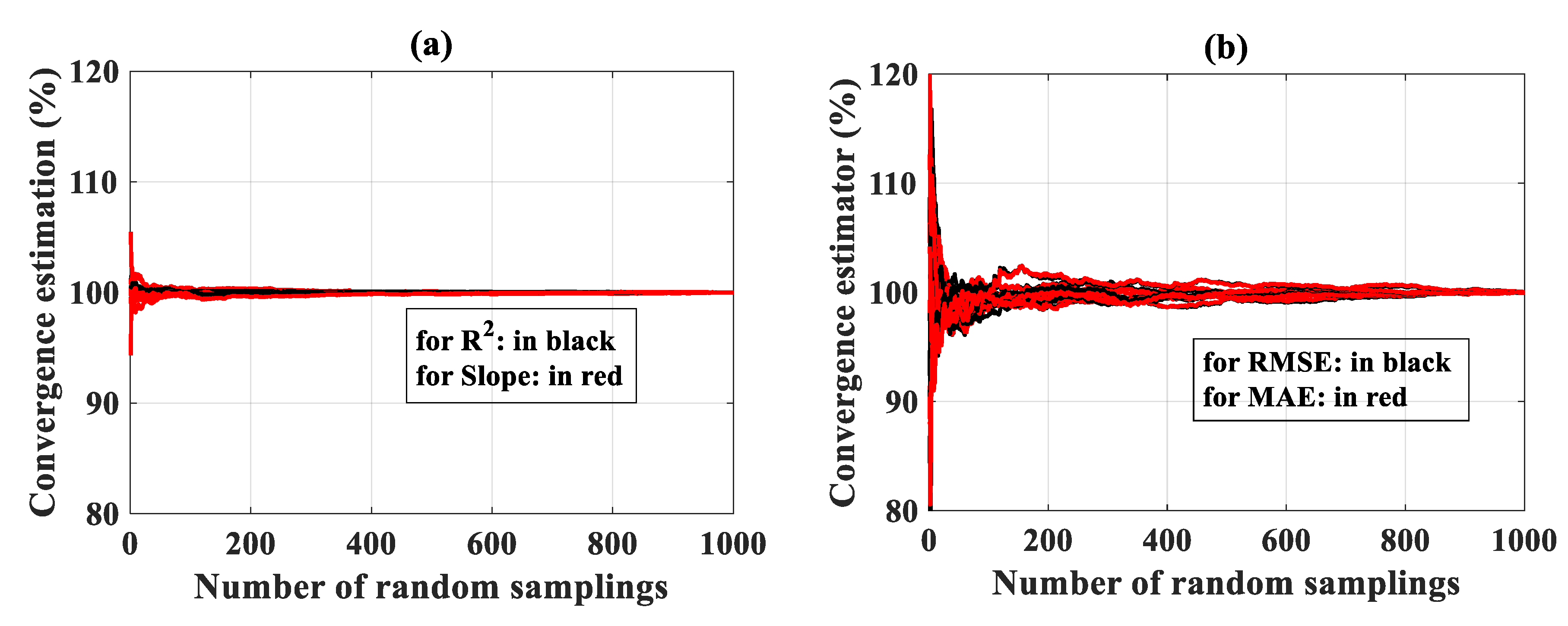
In order to evaluate the random sampling effect (i.e., variability in the input space), 1000 random combinations of data index were generated following a uniform distribution (to obtain the training and testing datasets with a ratio of 70/30). For each considered configuration of the ANN model (i.e., training function, activation function, number of neurons, etc.), 1000 Monte Carlo simulations were performed using these 1000 datasets. Therefore, 1000 values of R2, RMSE, MAE and Slope criteria were obtained by computing the deviation between the testing target and the corresponding output for each configuration of ANN model. The statistical convergence of error measurement criteria R2, Slope RMSE and MAE is analyzed in this section (also see Equation (3) for the calculation of that convergence). Figure 5a,b show the convergence estimation for (R2, Slope) and (RMSE, MAE) over 1000 Monte Carlo random sampling runs, respectively. In Figure 5, various curves are associated with the configurations of the parametric study. Figure 5 shows that R2 and Slope exhibit a lower order of fluctuation than do RMSE and MAE. This could be because RMSE and MAE measure the standard deviation of the prediction errors, whereas R2 and Slope indicate the degree of linear correlation between the target and predicted LBC. Consequently, random sampling was necessary, in order to estimate the statistical fluctuation with respect to all error measurement criteria, especially in terms of RMSE and MAE. It can be concluded that 1000 Monte Carlo random sampling runs is sufficient to obtain a representative convergence estimation, ready for subsequent statistical analysis, as seen in Figure 5b (a fluctuation of 1% around the mean value was reached from 900 simulations).
3.2. Results of Parametric Study
3.2.1. Results in Terms of Training Function
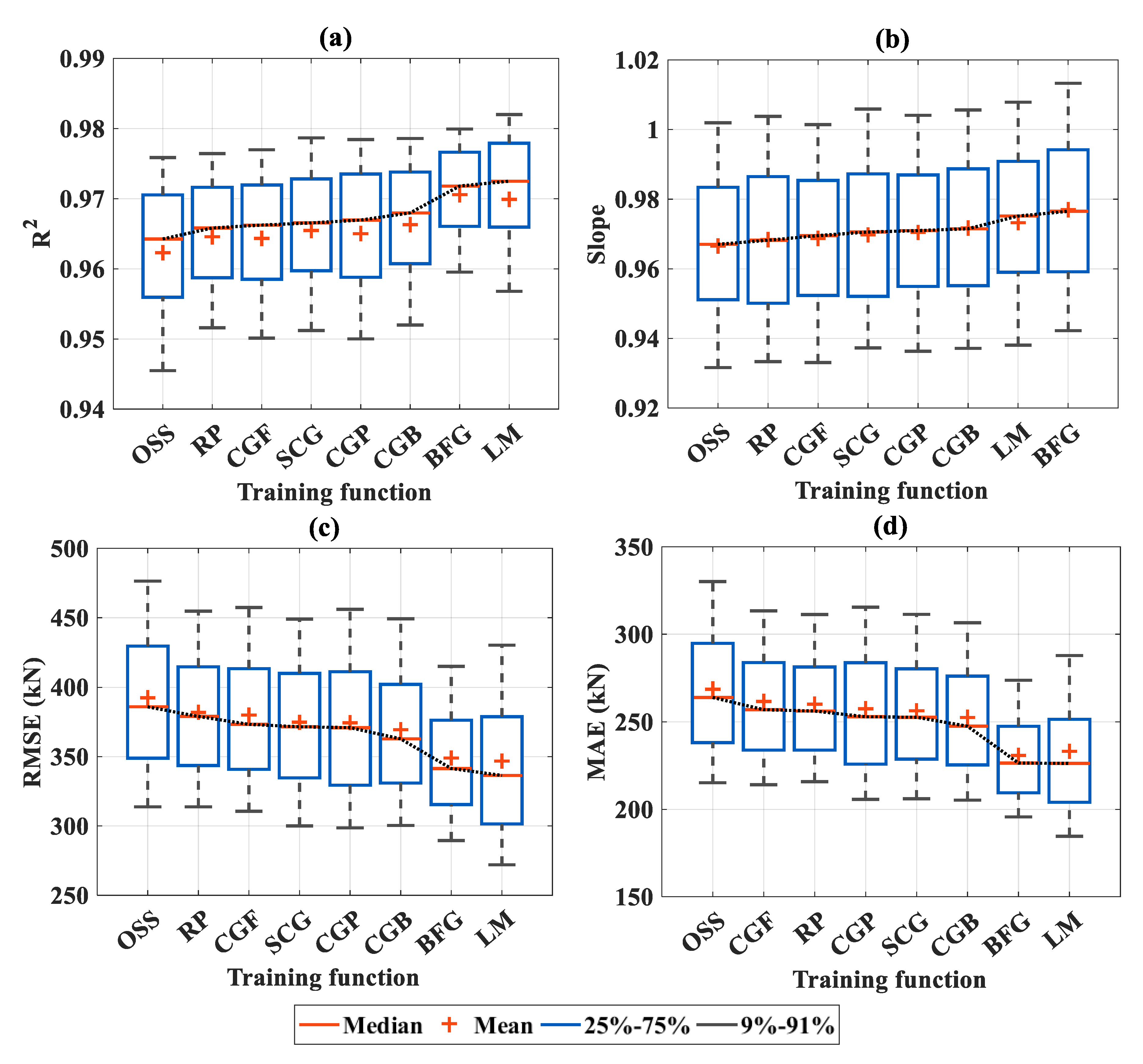
As reliable results were obtained as shown in Figure 5, this section presents the influence of using different training algorithms on the performance of the ANN model. To this end, other parameters, such as activation function, was fixed as tansig, number of neurons was fixed as 20 and cost function was fixed as mean square error. Figure 6a–d present the evaluation of R2, Slope, RMSE and MAE, respectively, as a function of the training algorithms. It should be noted that, as shown in Figure 6, the box plot was adopted to represent the probability distribution of error criteria over 1000 random sampling runs, including median, mean, 25%–75% and 9%–91% percentiles. The performance was ranked based on the median value of the distribution. Results showed that the BFG and LM algorithms exhibited the best performance, with respect to R2, Slope, RMSE and MAE, respectively. Furthermore, regarding R2, RMSE and MAE, BFG and LM also produced a lower level of fluctuation than other algorithms, as can be seen in terms of the 25%–75% percentiles of the distribution. Finally, the LM algorithm was selected as it provided the highest median value with respect to R2, and the lowest median value with respect to RMSE and MAE.
These observations of superior performance of the LM algorithm were in accordance with the literature. This algorithm was developed, in combining the conventional gradient descent technique and Gauss-Newton algorithm, in order to enhance the efficiency of the training process [54]. As a result, the LM technique has been widely used in various investigations in different areas of research [24,37,43,63].
3.2.2. Results in Terms of Activation Function
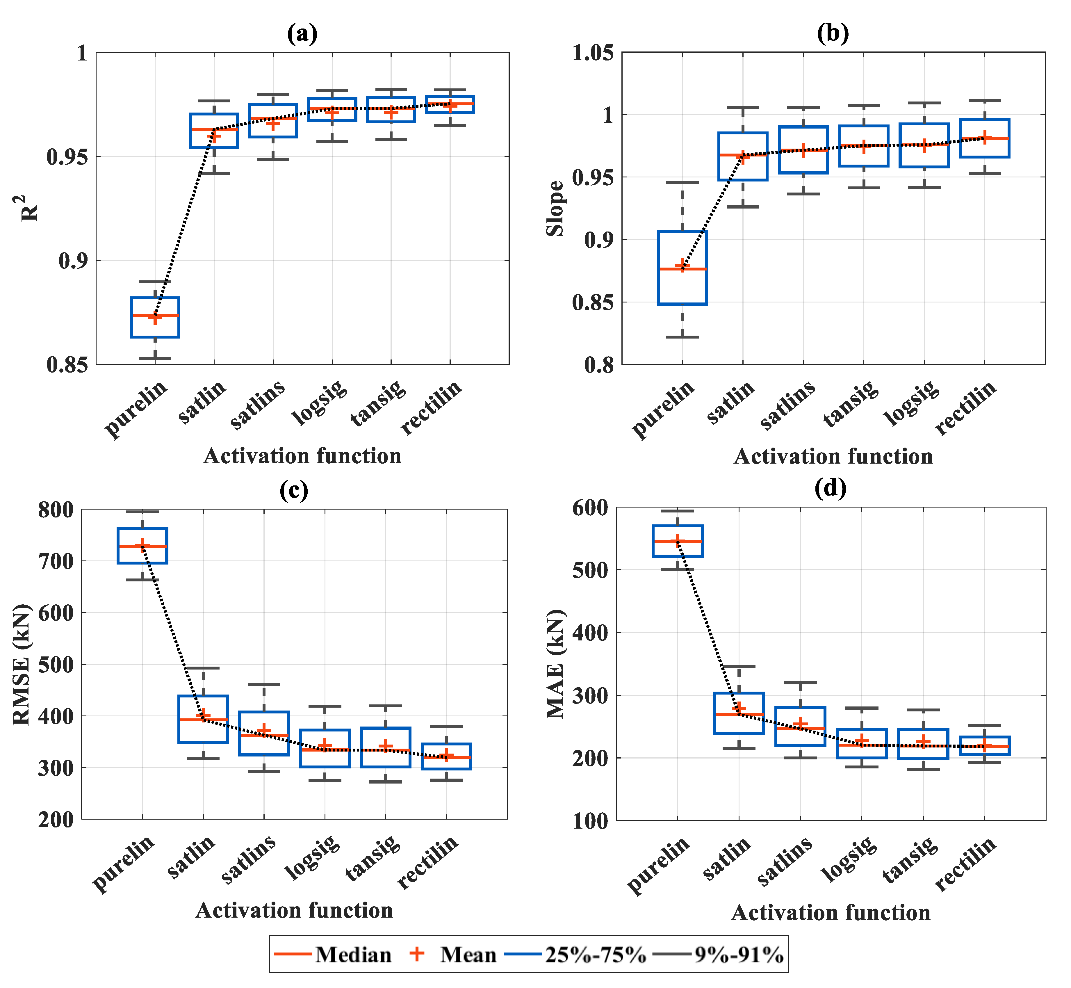
This section explores the influence of using different activation functions on the performance of the ANN model. To this end, other parameters such as training function was fixed as Levenberg-Marquardt, number of neurons was fixed as 20 and cost function was fixed as mean square error. Figure 7a–d show the box plot distribution of R2, Slope, RMSE and MAE, respectively, as a function of the six activation functions used. The presentation is the same as Figure 6—median, mean, 25–75% and 9–91% percentiles of the probability distribution over 1000 random sampling runs are highlighted. The performance was ranked based on the median value of the distribution. Results showed a poor performance for the purelin activation function. On the other hand, the logsig, tansig and rectilin offered superior performance for the ANN model, especially the rectilin activation function. Therefore, ultimately, the rectilin function was chosen as optimal.
3.2.3. Results in Terms of Number of Neurons
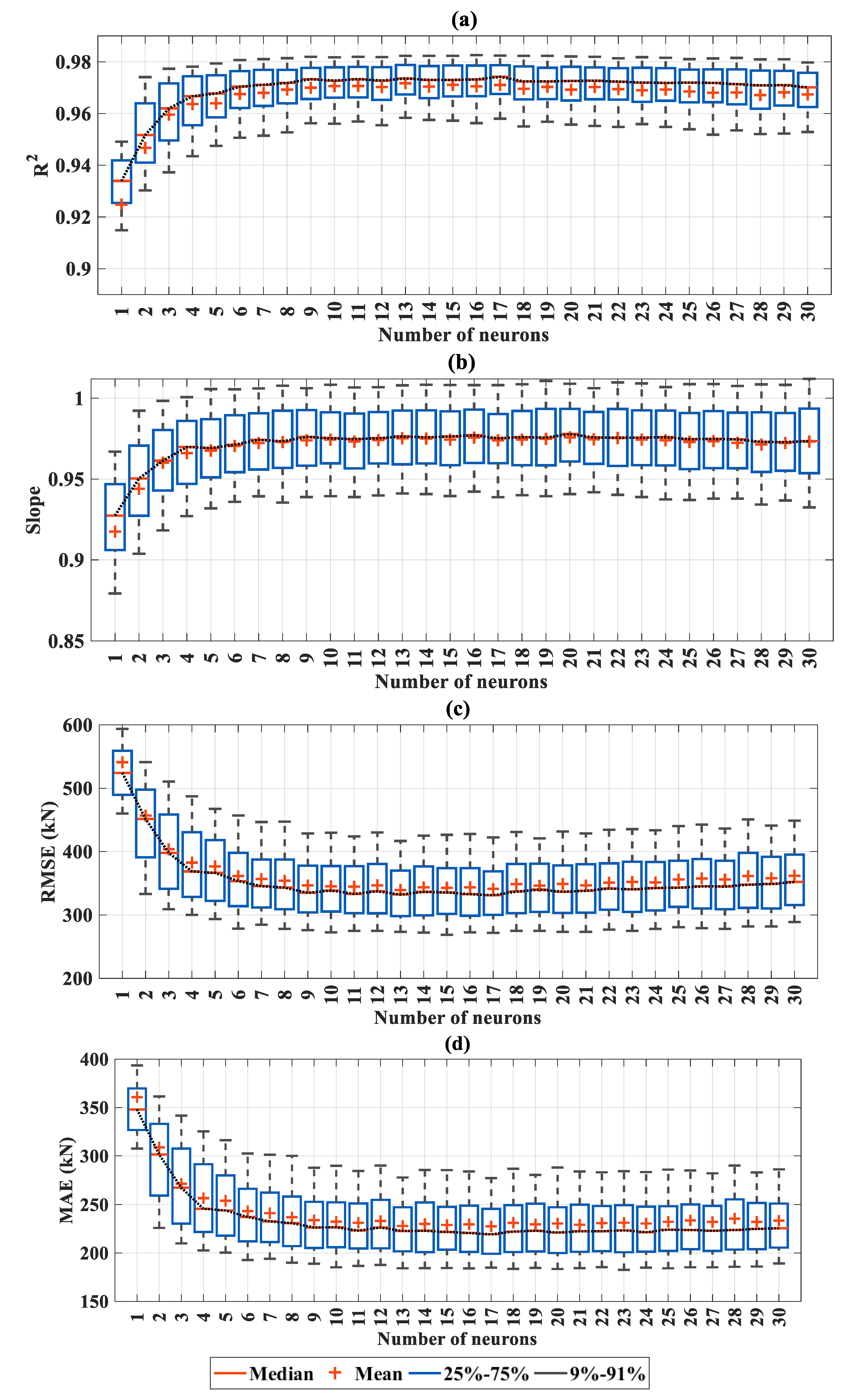
In this section, the influence of the number of neurons in the hidden layer on the performance of the ANN model is explored. To this end, other parameters such as training function was fixed as Levenberg-Marquardt, activation function was fixed as tansig and cost function was fixed as mean square error. Figure 8a–d show the box plot distribution of R2, Slope, RMSE and MAE, respectively, as a function of number of neurons, which was ranked from one to 30 with a resolution of one. The presentation is the same as in Figure 6: median, mean, 25–75% and 9–91% percentiles of the probability distribution over 1000 random sampling runs are shown. Results showed that a small number of neurons (i.e., fewer than five) gave a poor performance for the ANN model, with respect to all error measurement criteria (in both median and standard deviation). However, all the median values formed a concave curve, which indicated greatest performance around 15 artificial neurons. This observation confirmed that there is an optimal number of neurons for the given problem (i.e., beyond a certain point, increasing the number of neurons does not always improve performance). Therefore, the optimal number of neurons was finally chosen as 15.
The influence of cost functions on the performance of the ANN model was also evaluated. However, all considered cost functions produced similar results on the ANN’s performance. Mean square error was finally selected.
3.2.4. Optimal Parameters
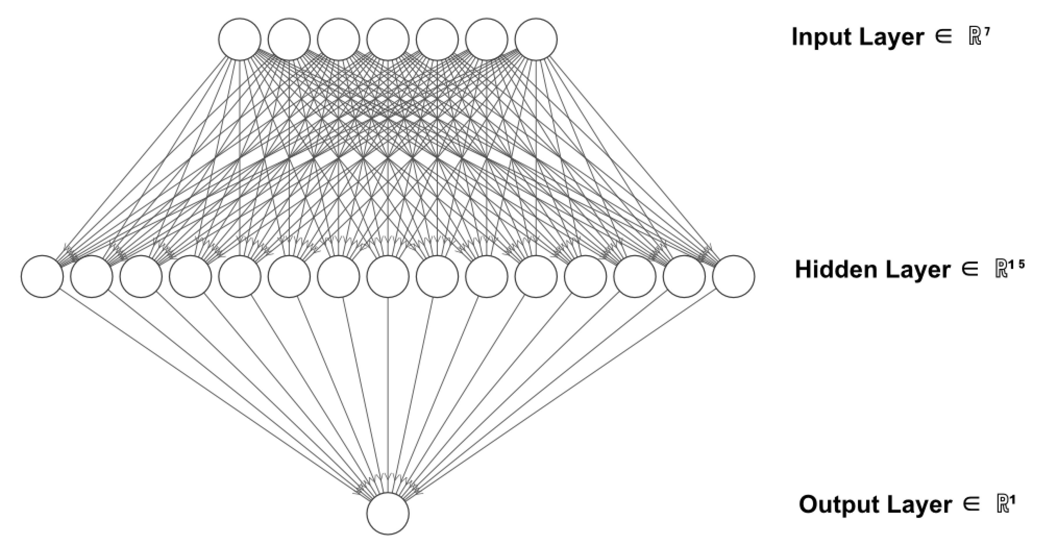
As calibrated previously, the final ANN model exhibits (see Figure 9):
- 15 neurons in the hidden layer;
- A rectilin activation function;
- A LM training algorithm;
- Mean square error as a cost function.
3.3. Analysis of Performance of the Final ANN Model
In this section, the final ANN model is presented, including regression, uncertainty and sensitivity analyses.
3.3.1. Regression Analysis
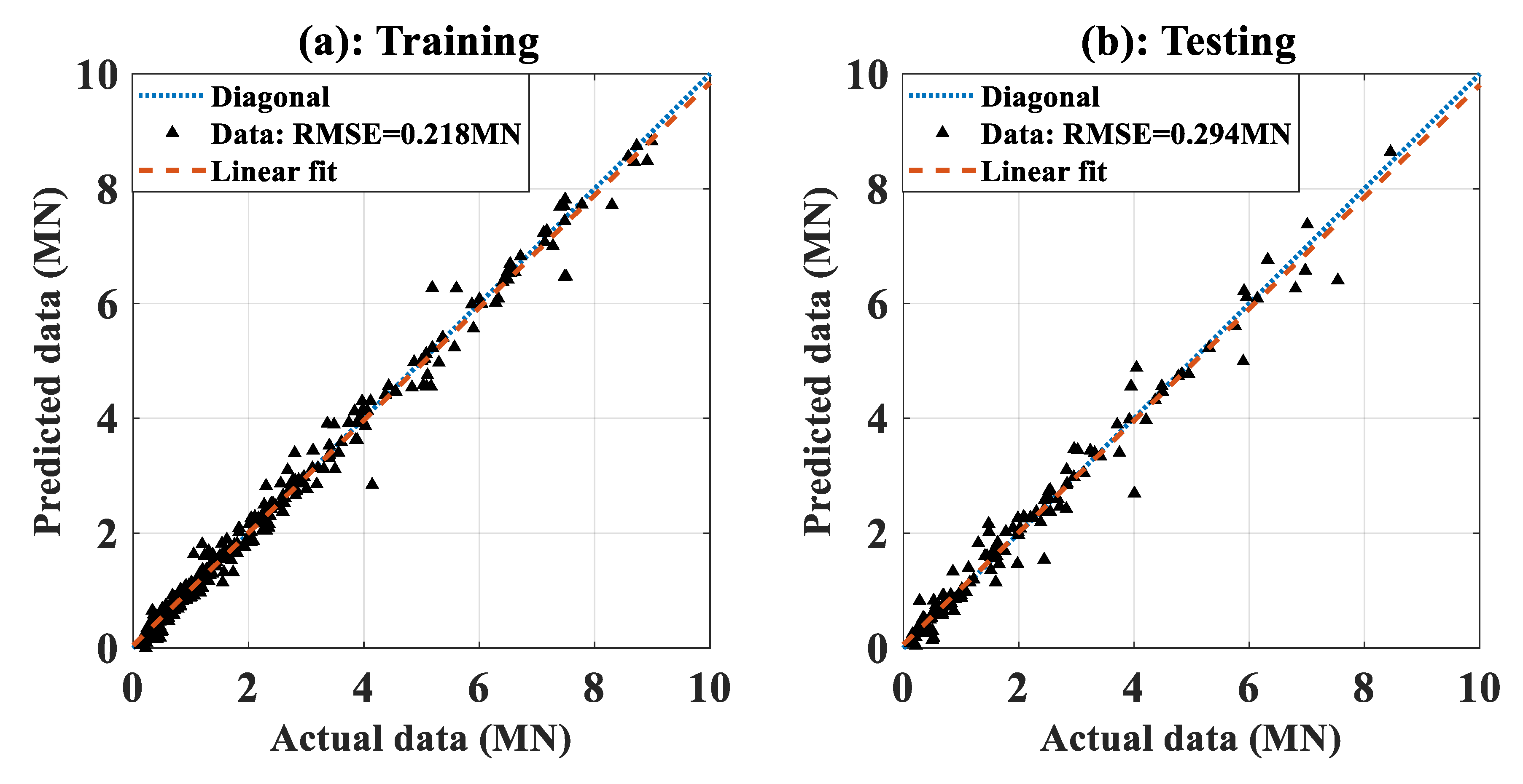
Figure 10a,b show the regression graphs between actual and predicted LBC of CFSS members using the training and testing data, respectively. All values of error measurement criteria are indicated in Table 2. In Figure 10, the linear fit is also presented, corresponding to a slope indicated in Table 2. A slope of 0.980 and 0.975 for the training and testing data, respectively, was obtained, corresponding to an angle between the linear fit line and the horizontal line of 44.429° and 44.263°, respectively. It is shown that for two data points, the linear fit is very close to the diagonal line (i.e., 45°), which confirmed that the coefficient of determination R2 is very good (i.e., R2 = 0.989 and 0.975, for training and testing data, respectively). In terms of RMSE and MAE, the ANN model exhibits a strong prediction performance. As indicated in Table 2, RMSE = 217.717 kN and 294.424 kN; MAE = 139.685 kN and 191.878 kN, using training and testing data, respectively. In addition, error analysis shows that the ErrorMean is close to zero, whereas an ErrorStD of 218.062 kN and 295.445 kN is explored. The values of ErrorMean close to zero indicates that there is no sign of over- or under-estimation of LBC, i.e., the data points are located uniformly around the diagonal line, as shown in Figure 10. Moreover, as observed in Figure 10, the values of the predicted LBC are not systematically too high or too low anywhere in the observation space. Indeed, the values of MAE show that the average magnitude of the residuals between the predicted and target LBC is lower than 200 kN. On the other hand, the standard deviation of such residuals is characterized by RMSE and ErrorStD (which approximately represent the same value, even though there is a different in the formula). As indicated in Table 2, the values of RMSE and ErrorStD are higher than ones of MAE (about 100 kN), showing that there is about 100 kN of variance in the individual residuals. From overall error measurements, good agreement between the predicted and the actual values of LBC of compressive CFSS members is obtained.
3.3.2. Uncertainty Analysis
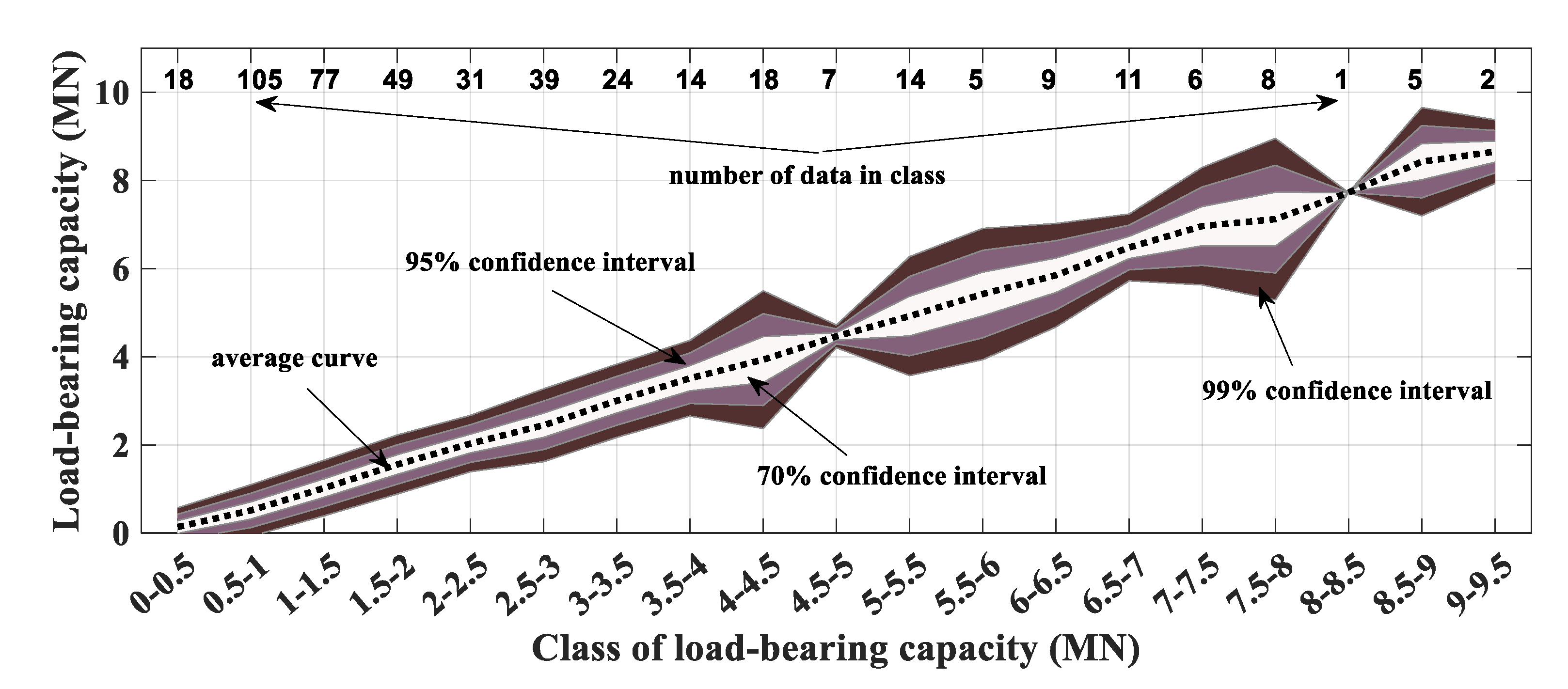
In addition, uncertainty analysis was performed to quantify the uncertainty of the ANN model during prediction. Nineteen classes of the target LBC were introduced, ranging from 0 to 9.5 MN with a resolution of 0.5 MN. The corresponding data in each level were deduced, and then used to compute the standard deviation. Figure 11 presents the 70%, 95% and 99% confidence intervals, together with the average curve, for the prediction of LBC using ANN, respectively. In this figure, the numbers of data points in each class are also indicated. When the LBC is lower than 4 MN, a low level of uncertainty is achieved. However, where the LBC is greater than 4 MN, the level of uncertainty is almost tripled. This is attributable to the fact that for an LBC lower than 4 MN, there are a high number of data points in each class—for instance, there are 105 data points between 0.5 and 1 MN. On the contrary, not many data points are distributed when the LBC is greater than 4 MN. Such an investigation could point out the current limitations of the model. In future research projects, more data points should be considered in order to obtain reliable representation, especially for classes greater than 4 MN.
3.3.3. Sensitivity Analysis
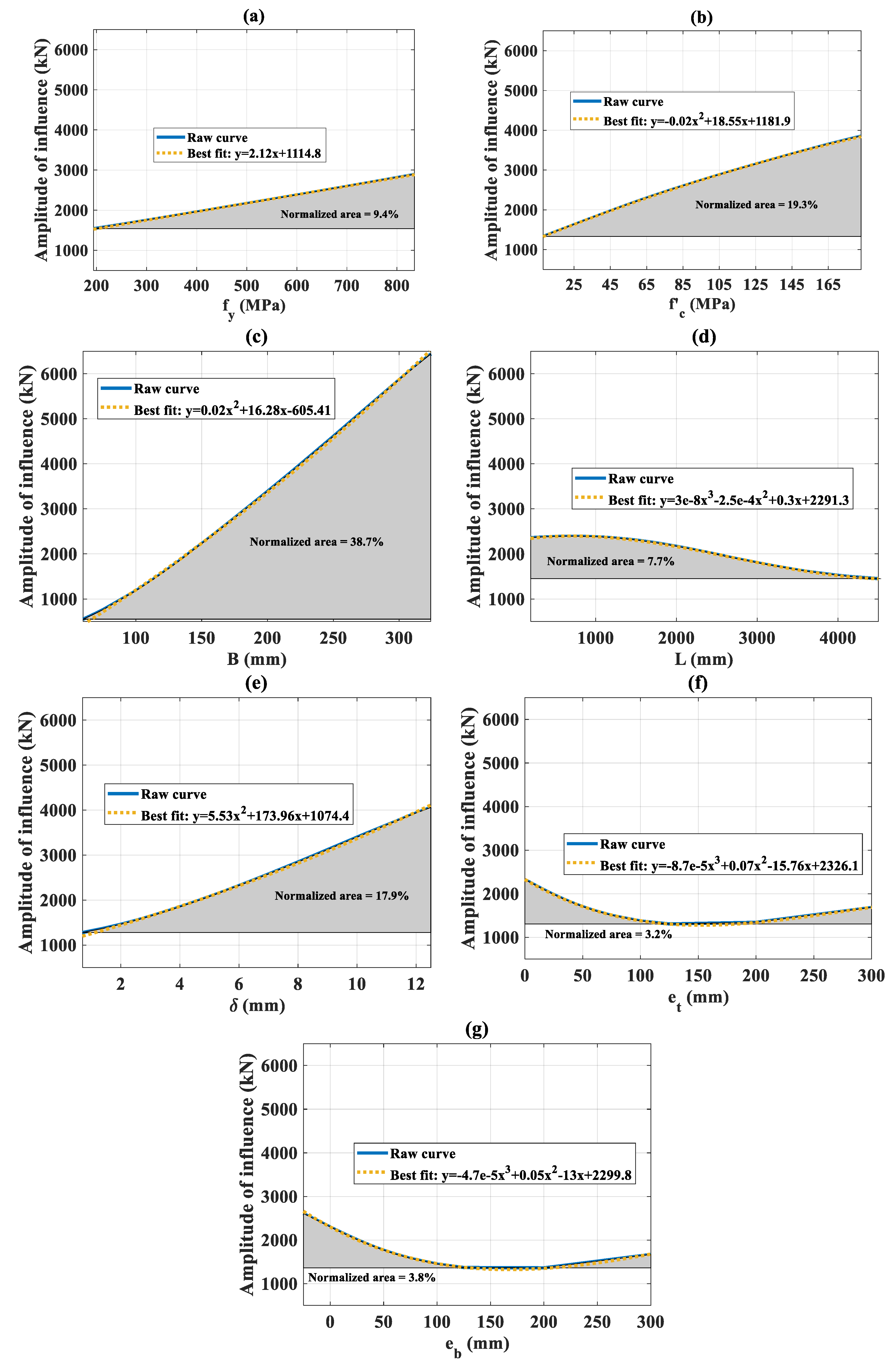
In this section, sensitivity analysis based on Individual Conditional Expectation (ICE) [98] is introduced, in order to explore the influence of each input variable on the output response of the ANN model. By definition, ICE is able to display how the output response changes when an input variable changes. Figure 12 shows the results of sensitivity analysis for each input variable, including the raw curve obtained by ICE, the most appropriate fit of the raw curve and the normalized area of the covered surface. It demonstrates that all input variables have an impact on the LBC of CFSS members, but to varying degrees and with differing effects. In terms of positive effect, the LBC of CFSS members increases with increasing fy following a linear equation; f’c, B and δ following a nonlinear form. In terms of negative effect, the LBC of CFSS members decreases with increasing L, et and eb following a nonlinear equation. In addition, it seems to have a minimum point in the graphs of eb and et. The descent stage allows confirming the negative effect of loading eccentricities on the LBC. However, the ascent stage should be checked in further studies, by investigating more configurations of loading eccentricities (see also Figure 2f,g). Regarding the normalized area of covered surface, B, f’c, δ, fy, L, eb and et exhibit 38.7%, 19.3%, 17.9%, 9.4%, 7.7%, 3.8% and 3.2%, respectively. This means that the most influential input variables are the geometric parameters of the steel tube and the compressive strength of the concrete core. These remarks are in close accordance with experimental studies in the literature [11,15,18,99]. Moreover, the sensitivity analysis indicates that linear correlation is not enough to describe the relationship between the inputs and the LBC, especially in the case of geometric parameters of the cross section. From physical point of view, such observation is in good agreement with the literature, as the LBC depend on the cross-sectional areas of the steel tube (As = (B−2δ)2) and the concrete core (Ac = B2 −(B−2δ)2), respectively [100,101]. Overall, without solving complex equations, an approach using an interpretable ANN model could indicate the relationships between input variables and output response in an efficient manner and avoiding excessive computational cost.
3.4. Discussion on Effect of Eccentric Loading
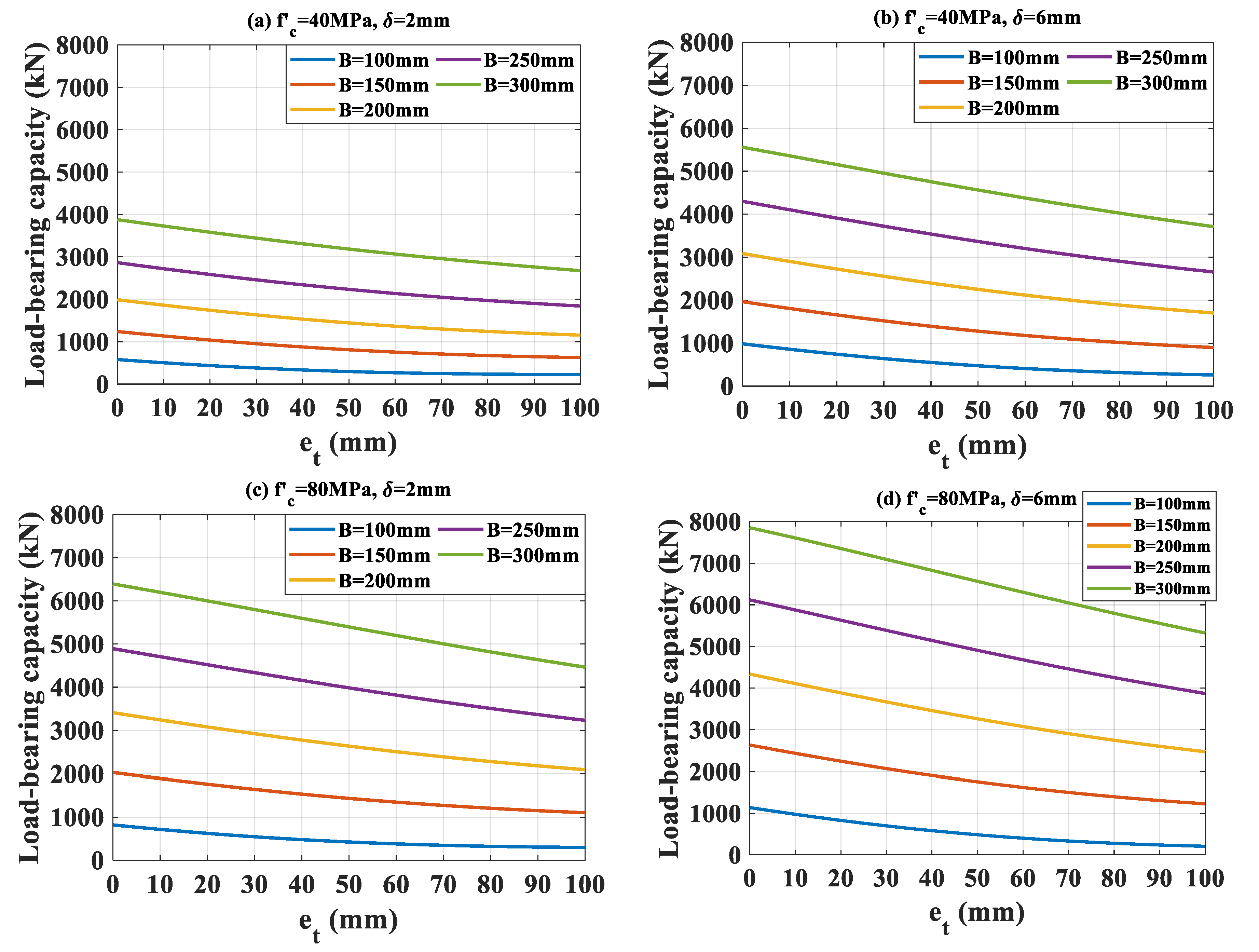
In addition to a reliable prediction of LBC, as presented above, the ANN model can also assist in creating LBC continuous curves (i.e., maps), within the ranges of the input variables adopted in this study. In this section, several scenarios concentrating on varying B, δ, f’c and et are presented, aiming to explore the effect of eccentric loading on the LBC of CFSS members. For the other input variables, L is fixed at 2000 mm, eb is fixed at 0, and fy is fixed at 400 MPa, respectively. Figure 13a shows the distribution of LBC as a function of et using f’c = 40 MPa, δ = 2 mm, B = 100, 150, 200, 250 and 300 mm, and et varies from 0 to 100 mm, respectively. Figure 13b shows the distribution of LBC as a function of et using f’c = 40 MPa but δ = 6 mm. Figure 13c shows the distribution of LBC as a function of et using δ = 2 mm, but f’c = 80 MPa. Figure 13d shows the distribution of LBC as a function of et using δ = 6 mm but f’c = 80 MPa. In all configurations, the LBC of CFSS members decreases when increasing et, which confirms the negative effect of this variable on the macroscopic behavior of the composite structures. These distributions also confirm the effect of B, δ and f’c as identified previously in the sensitivity analysis. The distributions presented herein aim exclusively to demonstrate the advantage of the proposed ANN model in providing efficient continuous mapping of LBC.
4. Conclusions and Outlook
In this work, a surrogate ANN model was proposed and optimized for prediction of the LBC of CFSS members. The ANN model was trained and validated against experimental data. A parametric study was performed to calibrate the parameters of the model, including the number of neurons, activation function, cost function and training algorithm, respectively. Statistical analysis based on Monte Carlo random sampling techniques was conducted to track the variability of the input space. The main conclusions of this study are as follows:
- For the considered problem, the optimal ANN model includes 15 neurons, rectilin activation function, mean squared error cost function and LM training algorithm;
- The proposed ANN model offers reliable prediction in terms of various performance indicators: R2 = 0.975, Slope = 0.975, RMSE = 294.424 kN and MAE = 191.878 kN, respectively;
- By performing sensitivity analysis based on the ICE technique, the geometric parameters of the cross section (B and δ), together with the compressive strength of the concrete (f‘c), have been found to be the most influential variables on the LBC;
- The effect of eccentric loading on the LBC of CFSS members is explored, within the ranges of the input variables adopted in this study;
- The proposed ANN model is able to assist the initial phase of research and design of CFSS members before any experiments are carried out.
However, there are several limitations of the current model, including the lack of data points in several classes of values of input variables. Updated data must be collected through further studies in order to enhance the model’s performance. For comparison and validation purposes, the effect of loading eccentricities should be compared with mathematical models and/or experimental results in further works. In addition, in terms of practical application, a Graphical User Interface, especially one based on Microsoft Excel, should be developed and provided for researchers and engineers, and to support the teaching and interpretation of the compressive behavior of CFSS members.
Author Contributions
Conceptualization, T.-T.L.; methodology, T.-T.L.; software, T.-T.L.; validation, T.-T.L.; investigation, T.-T.L.; writing—original draft preparation, T.-T.L.; writing—review and editing, T.-T.L.; funding acquisition, T.-T.L. All authors have read and agreed to the published version of the manuscript.
Funding
This research received no external funding.
Conflicts of Interest
The authors declare that there is no conflict of interest.
Data Availability
The raw/processed data required to reproduce these findings will be made available on request.
References
- Gupta, P.K.; Ahuja, A.K.; Khaudhair, Z.A. Modelling, verification and investigation of behaviour of circular CFST columns. Struct. Concr. 2014, 15, 340–349. [Google Scholar] [CrossRef]
- Han, L.-H.; Li, W.; Bjorhovde, R. Developments and advanced applications of concrete-filled steel tubular (CFST) structures: Members. J. Constr. Steel Res. 2014, 100, 211–228. [Google Scholar] [CrossRef]
- An, Y.F.; Han, L.H. Behaviour of concrete-encased CFST columns under combined compression and bending. J. Constr. Steel Res. 2014, 101, 314–330. [Google Scholar] [CrossRef]
- Güneyisi, E.M.; Gültekin, A.; Mermerdaş, K. Ultimate capacity prediction of axially loaded CFST short columns. Int. J. Steel Struct. 2016, 16, 99–114. [Google Scholar] [CrossRef]
- Lee, S.H.; Uy, B.; Kim, S.H.; Choi, Y.H.; Choi, S.M. Behavior of high-strength circular concrete-filled steel tubular (CFST) column under eccentric loading. J. Constr. Steel Res. 2011, 67, 1–13. [Google Scholar] [CrossRef]
- Tran, V.Q.; Nguyen, H.L.; Dao, V.D.; Hilloulin, B.; Nguyen, L.K.; Nguyen, Q.H.; Le, T.-T.; Ly, H.-B. Temperature effects on chloride binding capacity of cementitious materials. Mag. Concr. Res. 2019, 1–39, Ahead of Print. [Google Scholar] [CrossRef]
- Ly, H.-B.; Pham, B.T.; Dao, D.V.; Le, V.M.; Le, L.M.; Le, T.-T. Improvement of ANFIS Model for Prediction of Compressive Strength of Manufactured Sand Concrete. Appl. Sci. 2019, 9, 3841. [Google Scholar] [CrossRef] [Green Version]
- Lai, M.H.; Ho, J.C.M. Effect of continuous spirals on uni-axial strength and ductility of CFST columns. J. Constr. Steel Res. 2015, 104, 235–249. [Google Scholar] [CrossRef]
- Abramski, M. Load-carrying capacity of axially loaded concrete-filled steel tubular columns made of thin tubes. Arch. Civil Mech. Eng. 2018, 18, 902–913. [Google Scholar] [CrossRef]
- Mieloszyk, E.; Abramski, M.; Milewska, A. CFGFRPT Piles with a Circular Cross-Section and their Application in Offshore Structures. Pol. Marit. Res. 2019, 26, 128–137. [Google Scholar] [CrossRef] [Green Version]
- Tomii, M.; Yoshimura, K.; Morishita, Y. Experimental Studies on Concrete-Filled Steel Tubular Stub Columns under Concentric Loading; ASCE: Washington, DC, USA, 1977; pp. 718–741. [Google Scholar]
- Aslani, F.; Uy, B.; Tao, Z.; Mashiri, F. Behaviour and design of composite columns incorporating compact high-strength steel plates. J. Constr. Steel Res. 2015, 107, 94–110. [Google Scholar] [CrossRef]
- Chen, C.-C.; Ko, J.-W.; Huang, G.-L.; Chang, Y.-M. Local buckling and concrete confinement of concrete-filled box columns under axial load. J. Constr. Steel Res. 2012, 78, 8–21. [Google Scholar] [CrossRef]
- Khan, M.; Uy, B.; Tao, Z.; Mashiri, F. Behaviour and design of short high-strength steel welded box and concrete-filled tube (CFT) sections. Eng. Struct. 2017, 147, 458–472. [Google Scholar] [CrossRef]
- Xiong, M.-X.; Xiong, D.-X.; Liew, J.Y.R. Axial performance of short concrete filled steel tubes with high- and ultra-high- strength materials. Eng. Struct. 2017, 136, 494–510. [Google Scholar] [CrossRef]
- Du, Y.; Chen, Z.; Yu, Y. Behavior of rectangular concrete-filled high-strength steel tubular columns with different aspect ratio. Thin-Walled Struct. 2016, 109, 304–318. [Google Scholar] [CrossRef]
- Yan, J.-B.; Dong, X.; Wang, T. Axial compressive behaviours of square CFST stub columns at low temperatures. J. Constr. Steel Res. 2020, 164, 105812. [Google Scholar] [CrossRef]
- Qu, X.; Chen, Z.; Sun, G. Experimental study of rectangular CFST columns subjected to eccentric loading. Thin-Walled Struct. 2013, 64, 83–93. [Google Scholar] [CrossRef]
- Espinos, A.; Romero, M.L.; Portolés, J.M.; Hospitaler, A. Ambient and fire behavior of eccentrically loaded elliptical slenderconcrete-filled tubular columns. J. Constr. Steel Res. 2014, 100, 97–107. [Google Scholar] [CrossRef]
- Shen, Q.; Wang, J.; Wang, W.; Wang, Z. Performance and design of eccentrically-loaded concrete-filled round-ended elliptical hollow section stub columns. J. Constr. Steel Res. 2018, 150, 99–114. [Google Scholar] [CrossRef]
- McCann, F. Concrete-filled elliptical section steel columns under concentric and eccentric loading. In Proceedings of the Eighth International Conference on Advances in Steel Structures, Lisbon, Portugal, 22–24 July 2015. [Google Scholar]
- Sarir, P.; Chen, J.; Asteris, P.G.; Armaghani, D.J.; Tahir, M.M. Developing GEP tree-based, neuro-swarm, and whale optimization models for evaluation of bearing capacity of concrete-filled steel tube columns. Eng. Comput. 2019. Online First Articles. [Google Scholar] [CrossRef]
- Asteris, P.G.; Armaghani, D.J.; Hatzigeorgiou, G.D.; Karayannis, C.G.; Pilakoutas, K. Predicting the shear strength of reinforced concrete beams using Artificial Neural Networks. Comput. Concr. 2019, 24, 469–488. [Google Scholar] [CrossRef]
- Tran, V.-L.; Thai, D.-K.; Kim, S.-E. Application of ANN in predicting ACC of SCFST column. Compos. Struct. 2019, 228, 111332. [Google Scholar] [CrossRef]
- Samuel, O.D.; Okwu, M.O. Comparison of Response Surface Methodology (RSM) and Artificial Neural Network (ANN) in modelling of waste coconut oil ethyl esters production. Energy Sources Part A Recovery, Util. Environ. Eff. 2019, 41, 1049–1061. [Google Scholar] [CrossRef]
- Li, M.; Wang, J. An Empirical Comparison of Multiple Linear Regression and Artificial Neural Network for Concrete Dam Deformation Modelling. Available online: https://www.hindawi.com/journals/mpe/2019/7620948/ (accessed on 7 May 2020).
- Chen, J.; de Hoogh, K.; Gulliver, J.; Hoffmann, B.; Hertel, O.; Ketzel, M.; Bauwelinck, M.; van Donkelaar, A.; Hvidtfeldt, U.A.; Katsouyanni, K.; et al. A comparison of linear regression, regularization, and machine learning algorithms to develop Europe-wide spatial models of fine particles and nitrogen dioxide. Environ. Int. 2019, 130, 104934. [Google Scholar] [CrossRef] [PubMed]
- Darji, M.P.; Dabhi, V.K.; Prajapati, H.B. Rainfall forecasting using neural network: A survey. In Proceedings of the 2015 International Conference on Advances in Computer Engineering and Applications, Ghaziabad, India, 19–20 March 2015; pp. 706–713. [Google Scholar]
- Zhu, Y.; Zabaras, N.; Koutsourelakis, P.-S.; Perdikaris, P. Physics-constrained deep learning for high-dimensional surrogate modeling and uncertainty quantification without labeled data. J. Comput. Phys. 2019, 394, 56–81. [Google Scholar] [CrossRef] [Green Version]
- Stewart, R.; Ermon, S. Label-Free Supervision of Neural Networks with Physics and Domain Knowledge. arXiv 2016, arXiv:1609.05566 [cs]. [Google Scholar]
- Berg, J.; Nyström, K. A unified deep artificial neural network approach to partial differential equations in complex geometries. Neurocomputing 2018, 317, 28–41. [Google Scholar] [CrossRef] [Green Version]
- Nguyen, H.Q.; Ly, H.-B.; Tran, V.Q.; Nguyen, T.-A.; Le, T.-T.; Pham, B.T. Optimization of Artificial Intelligence System by Evolutionary Algorithm for Prediction of Axial Capacity of Rectangular Concrete Filled Steel Tubes under Compression. Materials 2020, 13, 1205. [Google Scholar] [CrossRef] [Green Version]
- Naderpour, H.; Poursaeidi, O.; Ahmadi, M. Shear resistance prediction of concrete beams reinforced by FRP bars using artificial neural networks. Measurement 2018, 126, 299–308. [Google Scholar] [CrossRef]
- Ahmadi, M.; Naderpour, H.; Kheyroddin, A. Utilization of artificial neural networks to prediction of the capacity of CCFT short columns subject to short term axial load. Arch. Civil Mech. Eng. 2014, 14, 510–517. [Google Scholar] [CrossRef]
- Cevik, A.; Kurtoğlu, A.E.; Bilgehan, M.; Gülşan, M.E.; Albegmprli, H.M. Support vector machines in structural engineering: A review. J. Civil Eng. Manag. 2015, 21, 261–281. [Google Scholar] [CrossRef]
- David, A.; Kurtoğlu, A.E.; Thaveeporn, P. Predicting the Outcome of Construction Litigation Using Boosted Decision Trees. J. Comput. Civil Eng. 2005, 19, 387–393. [Google Scholar] [CrossRef]
- Zhou, Y.; Li, S.; Zhou, C.; Luo, B. Intelligent Approach Based on Random Forest for Safety Risk Prediction of Deep Foundation Pit in Subway Stations. J. Comput. Civil Eng. 2019, 33, 05018004. [Google Scholar] [CrossRef]
- Naderpour, H.; Kheyroddin, A.; Amiri, G.G. Prediction of FRP-confined compressive strength of concrete using artificial neural networks. Compos. Struct. 2010, 92, 2817–2829. [Google Scholar] [CrossRef]
- Le, T.-T.; Pham, B.T.; Le, V.M.; Ly, H.-B.; Le, L.M. A Robustness Analysis of Different Nonlinear Autoregressive Networks Using Monte Carlo Simulations for Predicting High Fluctuation Rainfall. In Micro-Electronics and Telecommunication Engineering; Sharma, D.K., Balas, V.E., Son, L.H., Sharma, R., Cengiz, K., Eds.; Springer: Singapore, 2020; pp. 205–212. [Google Scholar]
- Le, V.M.; Pham, B.T.; Le, T.-T.; Ly, H.-B.; Le, L.M. Daily Rainfall Prediction Using Nonlinear Autoregressive Neural Network. In Micro-Electronics and Telecommunication Engineering; Sharma, D.K., Balas, V.E., Son, L.H., Sharma, R., Cengiz, K., Eds.; Springer: Singapore, 2020; pp. 213–221. [Google Scholar]
- Zhang, J.; Denavit, M.D.; Hajjar, J.F.; Lu, X. Bond Behavior of Concrete-Filled Steel Tube (CFT) Structures. Eng. J. Am. Inst. Steel Constr. 2012, 49, 169–185. [Google Scholar]
- Denavit, M.D.; Hajjar, J.F. Characterization of Behavior of Steel-Concrete Composite Members and Frames with Applications for Design; Newmark Structural Engineering Laboratory; University of Illinois at Urbana-Champaign: Urbana, IL, USA, 2014. [Google Scholar]
- Denavit, M.D.; Hajjar, J.F.; Perea, T.; Leon, R.T. Stability Analysis and Design of Composite Structures. J. Struct. Eng. 2016, 142, 04015157. [Google Scholar] [CrossRef]
- Wang, P.; Liu, Z.; Gao, R.X.; Guo, Y. Heterogeneous data-driven hybrid machine learning for tool condition prognosis. CIRP Ann. 2019, 68, 455–458. [Google Scholar] [CrossRef]
- Busse, L.M.; Buhmann, J.M. Model-Based Clustering of Inhomogeneous Paired Comparison Data. In Proceedings of the Similarity-Based Pattern Recognition, Venice, Italy, 28–30 September 2011; Pelillo, M., Hancock, E.R., Eds.; Springer: Berlin/Heidelberg, Germany, 2011; pp. 207–221. [Google Scholar]
- Bühlmann, P.; Meinshausen, N. Magging: Maximin Aggregation for Inhomogeneous Large-Scale Data; IEEE: Piscataway, NJ, USA, 2016; Volume 104, pp. 126–135. [Google Scholar] [CrossRef] [Green Version]
- McCulloch, W.S.; Pitts, W. A logical calculus of the ideas immanent in nervous activity. Bull. Math. Biophys. 1943, 5, 115–133. [Google Scholar] [CrossRef]
- Pham, B.T.; Nguyen, M.D.; Ly, H.-B.; Pham, T.A.; Hoang, V.; Van Le, H.; Le, T.-T.; Nguyen, H.Q.; Bui, G.L. Development of Artificial Neural Networks for Prediction of Compression Coefficient of Soft Soil. In CIGOS 2019, Innovation for Sustainable Infrastructure; Ha-Minh, C., Dao, D.V., Benboudjema, F., Derrible, S., Huynh, D.V.K., Tang, A.M., Eds.; Springer: Singapore, 2020; pp. 1167–1172. [Google Scholar]
- Pham, B.T.; Nguyen, M.D.; Dao, D.V.; Prakash, I.; Ly, H.-B.; Le, T.-T.; Ho, L.S.; Nguyen, K.T.; Ngo, T.Q.; Hoang, V.; et al. Development of artificial intelligence models for the prediction of Compression Coefficient of soil: An application of Monte Carlo sensitivity analysis. Sci. Total Environ. 2019, 679, 172–184. [Google Scholar] [CrossRef]
- Le, T.-T.; Pham, B.T.; Ly, H.-B.; Shirzadi, A.; Le, L.M. Development of 48-hour Precipitation Forecasting Model using Nonlinear Autoregressive Neural Network. In CIGOS 2019, Innovation for Sustainable Infrastructure; Ha-Minh, C., Dao, D.V., Benboudjema, F., Derrible, S., Huynh, D.V.K., Tang, A.M., Eds.; Springer: Singapore, 2020; pp. 1191–1196. [Google Scholar]
- Bayat, M.; Ghorbanpour, M.; Zare, R.; Jaafari, A.; Thai Pham, B. Application of artificial neural networks for predicting tree survival and mortality in the Hyrcanian forest of Iran. Comput. Electr. Agricult. 2019, 164, 104929. [Google Scholar] [CrossRef]
- Chang, K.-T.; Merghadi, A.; Yunus, A.P.; Pham, B.T.; Dou, J. Evaluating scale effects of topographic variables in landslide susceptibility models using GIS-based machine learning techniques. Sci. Rep. 2019, 9, 1–21. [Google Scholar] [CrossRef] [PubMed] [Green Version]
- Witten, I.H.; Frank, E.; Hall, M.A.; Pal, C.J. Data Mining: Practical Machine Learning Tools and Techniques; Morgan Kaufmann: Burlington, MA, USA, 2016; ISBN 978-0-12-804357-8. [Google Scholar]
- Phong, T.V.; Phan, T.T.; Prakash, I.; Singh, S.K.; Shirzadi, A.; Chapi, K.; Ly, H.-B.; Ho, L.S.; Quoc, N.K.; Pham, B.T. Landslide susceptibility modeling using different artificial intelligence methods: A case study at Muong Lay district, Vietnam. Geocarto Int. 2019, 0, 1–24. [Google Scholar] [CrossRef]
- Ly, H.-B.; Monteiro, E.; Le, T.-T.; Le, V.M.; Dal, M.; Regnier, G.; Pham, B.T. Prediction and Sensitivity Analysis of Bubble Dissolution Time in 3D Selective Laser Sintering Using Ensemble Decision Trees. Materials 2019, 12, 1544. [Google Scholar] [CrossRef] [PubMed] [Green Version]
- Dao, D.V.; Ly, H.-B.; Trinh, S.H.; Le, T.-T.; Pham, B.T. Artificial Intelligence Approaches for Prediction of Compressive Strength of Geopolymer Concrete. Materials 2019, 12, 983. [Google Scholar] [CrossRef] [PubMed] [Green Version]
- Madani, K. Industrial and real world applications of artificial neural networks Illusion or reality. In Informatics in Control, Automation and Robotics I; Braz, J., Araújo, H., Vieira, A., Encarnação, B., Eds.; Springer: Dordrecht, The Netherlands, 2006; pp. 11–26. [Google Scholar]
- Neto, P.; Pereira, D.; Pires, J.N.; Moreira, A.P. Real-time and continuous hand gesture spotting: An approach based on artificial neural networks. In Proceedings of the 2013 IEEE International Conference on Robotics and Automation, Karlsruhe, Germany, 6–10 May 2013; pp. 178–183. [Google Scholar]
- Piotrowski, A.P.; Napiorkowski, J.J. A comparison of methods to avoid overfitting in neural networks training in the case of catchment runoff modelling. J. Hydrol. 2013, 476, 97–111. [Google Scholar] [CrossRef]
- Rusiecki, A.; Kordos, M.; Kamiński, T.; Greń, K. Training Neural Networks on Noisy Data. In Proceedings of the Artificial Intelligence and Soft Computing, Zakopane, Poland, 1–5 June 2014; Rutkowski, L., Korytkowski, M., Scherer, R., Tadeusiewicz, R., Zadeh, L.A., Zurada, J.M., Eds.; Springer International Publishing: Cham, Switzerland, 2014; pp. 131–142. [Google Scholar]
- Qi, C.; Chen, Q.; Dong, X.; Zhang, Q.; Yaseen, Z.M. Pressure drops of fresh cemented paste backfills through coupled test loop experiments and machine learning techniques. Powder Technol. 2019, 361, 748–758. [Google Scholar] [CrossRef]
- Bui, K.-T.T.; Tien Bui, D.; Zou, J.; Van Doan, C.; Revhaug, I. A novel hybrid artificial intelligent approach based on neural fuzzy inference model and particle swarm optimization for horizontal displacement modeling of hydropower dam. Neural Comput. Appl. 2018, 29, 1495–1506. [Google Scholar] [CrossRef]
- Asteris, P.G.; Roussis, P.C.; Douvika, M.G. Feed-Forward Neural Network Prediction of the Mechanical Properties of Sandcrete Materials. Sensors 2017, 17, 1344. [Google Scholar] [CrossRef] [Green Version]
- Ly, H.-B.; Le, T.-T.; Le, L.M.; Tran, V.Q.; Le, V.M.; Vu, H.-L.T.; Nguyen, Q.H.; Pham, B.T. Development of Hybrid Machine Learning Models for Predicting the Critical Buckling Load of I-Shaped Cellular Beams. Appl. Sci. 2019, 9, 5458. [Google Scholar] [CrossRef] [Green Version]
- Asteris, P.G.; Nikoo, M. Artificial bee colony-based neural network for the prediction of the fundamental period of infilled frame structures. Neural Comput. Appl. 2019, 31, 4837–4847. [Google Scholar] [CrossRef]
- Reynaldi, A.; Lukas, S.; Margaretha, H. Backpropagation and Levenberg-Marquardt Algorithm for Training Finite Element Neural Network. In Proceedings of the 2012 Sixth UKSim/AMSS European Symposium on Computer Modeling and Simulation, Valetta, Malta, 14–16 November 2012; pp. 89–94. [Google Scholar]
- Mizutani, E.; Dreyfus, S.E.; Nishio, K. On derivation of MLP backpropagation from the Kelley-Bryson optimal-control gradient formula and its application. In Proceedings of the Proceedings of the IEEE-INNS-ENNS International Joint Conference on Neural Networks. IJCNN 2000. Neural Computing: New Challenges and Perspectives for the New Millennium, Como, Italy, 27 July 2000; Volume 2, pp. 167–172. [Google Scholar]
- Aggarwal, C.C. Machine Learning with Shallow Neural Networks. In Neural Networks and Deep Learning: A Textbook; Aggarwal, C.C., Ed.; Springer International Publishing: Cham, Switzerland, 2018; pp. 53–104. ISBN 978-3-319-94463-0. [Google Scholar]
- Nair, V.; Hinton, G.E. Rectified linear units improve restricted boltzmann machines. In Proceedings of the 27th International Conference on International Conference on Machine Learning; Omnipress, Haifa, Israel, 21–24 June 2010; pp. 807–814. [Google Scholar]
- Vogl, T.P.; Mangis, J.K.; Rigler, A.K.; Zink, W.T.; Alkon, D.L. Accelerating the convergence of the back-propagation method. Biol. Cybern. 1988, 59, 257–263. [Google Scholar] [CrossRef]
- Haykin, S. Neural Networks: A Comprehensive Foundation, 2nd ed.; Prentice Hall: Upper Saddle River, NJ, USA, 1998; ISBN 978-0-13-273350-2. [Google Scholar]
- Wu, H. Global stability analysis of a general class of discontinuous neural networks with linear growth activation functions. Inf. Sci. 2009, 179, 3432–3441. [Google Scholar] [CrossRef]
- Wackerly, D.; Mendenhall, W.; Scheaffer, R.L. Mathematical Statistics with Applications, 7th ed.; Thomson Brooks/Cole: Belmont, CA, USA, 2008; ISBN 978-0-495-11081-1. [Google Scholar]
- Marquardt, D. An Algorithm for Least-Squares Estimation of Nonlinear Parameters. J. Soc. Ind. Appl. Math. 1963, 11, 431–441. [Google Scholar] [CrossRef]
- Møller, M.F. A scaled conjugate gradient algorithm for fast supervised learning. Neural Netw. 1993, 6, 525–533. [Google Scholar] [CrossRef]
- Gill, P.E.; Murray, W.; Wright, M.H. Practical Optimization; Emerald Group Publishing Limited: London, UK; New York, NY, USA, 1982; ISBN 978-0-12-283952-8. [Google Scholar]
- Riedmiller, M.; Braun, H. A direct adaptive method for faster backpropagation learning: The RPROP algorithm. In Proceedings of the IEEE International Conference on Neural Networks, San Francisco, CA, USA, 28 March–1 April 1993; Volume 1, pp. 586–591. [Google Scholar]
- Powell, M.J.D. Restart procedures for the conjugate gradient method. Math. Programm. 1977, 12, 241–254. [Google Scholar] [CrossRef]
- Scales, L.E. Introduction to Non-Linear Optimization, 1987th ed.; Springer: New York, NY, USA, 1987; ISBN 978-0-387-91252-3. [Google Scholar]
- Battiti, R. First- and Second-Order Methods for Learning: Between Steepest Descent and Newton’s Method. Neural Comput. 1992, 4, 141–166. [Google Scholar] [CrossRef]
- Le, T.T.; Guilleminot, J.; Soize, C. Stochastic continuum modeling of random interphases from atomistic simulations. Application to a polymer nanocomposite. Comp. Methods Appl. Mech. Eng. 2016, 303, 430–449. [Google Scholar] [CrossRef] [Green Version]
- Guilleminot, J.; Le, T.T.; Soize, C. Stochastic framework for modeling the linear apparent behavior of complex materials: Application to random porous materials with interphases. Acta Mech. Sinica 2013, 29, 773–782. [Google Scholar] [CrossRef] [Green Version]
- Dao, D.V.; Ly, H.-B.; Vu, H.-L.T.; Le, T.-T.; Pham, B.T. Investigation and Optimization of the C-ANN Structure in Predicting the Compressive Strength of Foamed Concrete. Materials 2020, 13, 1072. [Google Scholar] [CrossRef] [Green Version]
- Soize, C.; Desceliers, C.; Guilleminot, J.; Le, T.-T.; Nguyen, M.-T.; Perrin, G.; Allain, J.-M.; Gharbi, H.; Duhamel, D.; Funfschilling, C. Stochastic representations and statistical inverse identification for uncertainty quantification in computational mechanics. In Proceedings of the ECCOMAS Thematic Conference on Uncertainty Quantification in Computational Sciences and Engineering, Crete, Greece, 25–27 May 2015; pp. 1–26. [Google Scholar]
- Le, T.-T. Modélisation Stochastique, en Mécanique des Milieux Continus, de L’interphase Inclusion-Matrice à Partir de Simulations en Dynamique Moléculaire. Ph.D. Thesis, University of Paris-Est Marne-la-Vallée, Paris, France, 2015. [Google Scholar]
- Soize, C. A nonparametric model of random uncertainties for reduced matrix models in structural dynamics. Probab. Eng. Mech. 2000, 15, 277–294. [Google Scholar] [CrossRef] [Green Version]
- Soize, C. Random matrix theory for modeling uncertainties in computational mechanics. Comp. Methods Appl. Mech. Eng. 2005, 194, 1333–1366. [Google Scholar] [CrossRef] [Green Version]
- Dao, D.V.; Adeli, H.; Ly, H.-B.; Le, L.M.; Le, V.M.; Le, T.-T.; Pham, B.T. A Sensitivity and Robustness Analysis of GPR and ANN for High-Performance Concrete Compressive Strength Prediction Using a Monte Carlo Simulation. Sustainability 2020, 12, 830. [Google Scholar] [CrossRef] [Green Version]
- Qi, C.; Ly, H.-B.; Chen, Q.; Le, T.-T.; Le, V.M.; Pham, B.T. Flocculation-dewatering prediction of fine mineral tailings using a hybrid machine learning approach. Chemosphere 2020, 244, 125450. [Google Scholar] [CrossRef] [PubMed]
- Nguyen, H.-L.; Pham, B.T.; Son, L.H.; Thang, N.T.; Ly, H.-B.; Le, T.-T.; Ho, L.S.; Le, T.-H.; Tien Bui, D. Adaptive Network Based Fuzzy Inference System with Meta-Heuristic Optimizations for International Roughness Index Prediction. Appl. Sci. 2019, 9, 4715. [Google Scholar] [CrossRef] [Green Version]
- Nguyen, Q.H.; Ly, H.-B.; Le, T.-T.; Nguyen, T.-A.; Phan, V.-H.; Tran, V.Q.; Pham, B.T. Parametric Investigation of Particle Swarm Optimization for Improving Performance of Adaptive Neuro-Fuzzy Inference System in Determining Buckling Capacity of Circular Opening Steel Beams. Materials 2020, 13, 2210. [Google Scholar] [CrossRef]
- Pham, B.T.; Nguyen-Thoi, T.; Ly, H.-B.; Nguyen, M.D.; Al-Ansari, N.; Tran, V.-Q.; Le, T.-T. Extreme Learning Machine Based Prediction of Soil Shear Strength: A Sensitivity Analysis Using Monte Carlo Simulations and Feature Backward Elimination. Sustainability 2020, 12, 2339. [Google Scholar] [CrossRef] [Green Version]
- Pham, B.T.; Le, L.M.; Le, T.-T.; Bui, K.-T.T.; Le, V.M.; Ly, H.-B.; Prakash, I. Development of advanced artificial intelligence models for daily rainfall prediction. Atmos. Res. 2020, 237, 104845. [Google Scholar] [CrossRef]
- Ly, H.-B.; Le, L.M.; Phi, L.V.; Phan, V.-H.; Tran, V.Q.; Pham, B.T.; Le, T.-T.; Derrible, S. Development of an AI Model to Measure Traffic Air Pollution from Multisensor and Weather Data. Sensors 2019, 19, 4941. [Google Scholar] [CrossRef] [Green Version]
- Dao, D.V.; Jaafari, A.; Bayat, M.; Mafi-Gholami, D.; Qi, C.; Moayedi, H.; Phong, T.V.; Ly, H.-B.; Le, T.-T.; Trinh, P.T.; et al. A spatially explicit deep learning neural network model for the prediction of landslide susceptibility. Catena 2020, 188, 104451. [Google Scholar] [CrossRef]
- Ly, H.-B.; Le, T.-T.; Vu, H.-L.T.; Tran, V.Q.; Le, L.M.; Pham, B.T. Computational Hybrid Machine Learning Based Prediction of Shear Capacity for Steel Fiber Reinforced Concrete Beams. Sustainability 2020, 12, 2709. [Google Scholar] [CrossRef] [Green Version]
- Nguyen, H.-L.; Le, T.-H.; Pham, C.-T.; Le, T.-T.; Ho, L.S.; Le, V.M.; Pham, B.T.; Ly, H.-B. Development of Hybrid Artificial Intelligence Approaches and a Support Vector Machine Algorithm for Predicting the Marshall Parameters of Stone Matrix Asphalt. Appl. Sci. 2019, 9, 3172. [Google Scholar] [CrossRef] [Green Version]
- Goldstein, A.; Kapelner, A.; Bleich, J.; Pitkin, E. Peeking inside the black box: Visualizing statistical learning with plots of individual conditional expectation. J. Comput. Graph. Stat. 2015, 24, 44–65. [Google Scholar] [CrossRef]
- Han, L.-H.; Yao, G.-H. Influence of concrete compaction on the strength of concrete-filled steel RHS columns. J. Constr. Steel Res. 2003, 59, 751–767. [Google Scholar] [CrossRef]
- Eurocode 4. Design of Composite Steel and Concrete Structures. Part 1.1, General Rules and Rules for Buildings; European Committee for Standardization, British Standards Institution: London, UK, 2004. [Google Scholar]
- AISC. Specification for Structural Steel Buildings ANSI/AISC 360-16; American Institute of Steel Construction: Chicago, IL, USA, 2010. [Google Scholar]
Figure 1.
Diagram of a concrete-filled steel square hollow section (CFSS) member: (a) under eccentric loading; (b) square cross section (et and eb are defined based on the Oexey coordinate system, in this example, et is positive and eb is negative, respectively); and (c) load-axial shortening curve.

Figure 2.
Histogram of the data: (a) yield strength of steel tube, (b) compressive strength of concrete, (c) width of cross section, (d) length of column, (e) thickness of steel tube, (f) loading eccentricity at the top, (g) loading eccentricity at the bottom and (h) load-bearing capacity.
Figure 2.
Histogram of the data: (a) yield strength of steel tube, (b) compressive strength of concrete, (c) width of cross section, (d) length of column, (e) thickness of steel tube, (f) loading eccentricity at the top, (g) loading eccentricity at the bottom and (h) load-bearing capacity.

Figure 3.
Illustration of the ANN model involving one hidden layer.

Figure 4.
Activation functions used in this study: (a) tansig, (b) logsig, (c) purelin, (d) rectilin, (e) satlin and (f) satlins.
Figure 4.
Activation functions used in this study: (a) tansig, (b) logsig, (c) purelin, (d) rectilin, (e) satlin and (f) satlins.

Figure 5.
Statistical convergence for (a) R2 and Slope, (b) root mean square error (RMSE) and mean absolute error (MAE), over 1000 random sampling runs. Various curves are associated with the configurations of the parametric study.
Figure 5.
Statistical convergence for (a) R2 and Slope, (b) root mean square error (RMSE) and mean absolute error (MAE), over 1000 random sampling runs. Various curves are associated with the configurations of the parametric study.

Figure 6.
Evaluation of training algorithms: box plot over 1000 random sampling runs with respect to (a) R2, (b) Slope, (c) RMSE and (d) MAE.
Figure 6.
Evaluation of training algorithms: box plot over 1000 random sampling runs with respect to (a) R2, (b) Slope, (c) RMSE and (d) MAE.

Figure 7.
Evaluation of activation functions: box plot over 1000 random sampling runs with respect to (a) R2, (b) Slope, (c) RMSE and (d) MAE.
Figure 7.
Evaluation of activation functions: box plot over 1000 random sampling runs with respect to (a) R2, (b) Slope, (c) RMSE and (d) MAE.

Figure 8.
Evaluation of number of neurons: box plot over 1000 random sampling runs with respect to (a) R2, (b) Slope, (c) RMSE and (d) MAE.
Figure 8.
Evaluation of number of neurons: box plot over 1000 random sampling runs with respect to (a) R2, (b) Slope, (c) RMSE and (d) MAE.

Figure 9.
Final architecture of the Artificial Neural Network (ANN) model.

Figure 10.
Regression graphs between actual and predicted load-bearing capacity (LBC) using (a) training and (b) testing data.
Figure 10.
Regression graphs between actual and predicted load-bearing capacity (LBC) using (a) training and (b) testing data.

Figure 11.
Uncertainty analysis of the ANN model.

Figure 12.
Sensitivity analysis of (a) fy, (b) f’c, (c) B, (d) L, (e) δ, (f) et and (g) eb, on the output response from the ANN model.
Figure 12.
Sensitivity analysis of (a) fy, (b) f’c, (c) B, (d) L, (e) δ, (f) et and (g) eb, on the output response from the ANN model.

Figure 13.
(a–d) Effect of eccentric loading on the LBC of compressive CFSS members in different scenarios. The same limits are applied on the x- and y-axes.
Figure 13.
(a–d) Effect of eccentric loading on the LBC of compressive CFSS members in different scenarios. The same limits are applied on the x- and y-axes.


Table 1.
Initial statistical analysis of the database.
| Variable | Min | Mean | Max | StD | CV (%) | Symbol | Unit | Type |
|---|---|---|---|---|---|---|---|---|
| Yield strength of steel tube | 194.18 | 472.79 | 835.00 | 192.91 | 40.80 | fy | MPa | Input |
| Compressive strength of concrete | 7.90 | 59.84 | 183.00 | 36.50 | 61.00 | f’c | MPa | Input |
| Width of cross section | 60.00 | 147.18 | 324.00 | 56.86 | 38.63 | B | mm | Input |
| Length of column | 195.00 | 1426.55 | 4500.00 | 1110.43 | 77.84 | L | mm | Input |
| Thickness of steel tube | 0.70 | 4.88 | 12.50 | 2.17 | 44.40 | δ | mm | Input |
| Loading eccentricity at the top | 0.00 | 14.58 | 300.00 | 37.10 | 254.37 | et | mm | Input |
| Loading eccentricity at the bottom | −25.00 | 13.51 | 300.00 | 37.02 | 274.01 | eb | mm | Input |
| Load-bearing capacity | 105.40 | 2205.44 | 8990.00 | 2036.74 | 92.35 | Fn | kN | Target |
Table 2.
Summary of performance of the ANN model.
| Data Used | RMSE (kN) | MAE (kN) | Error Mean (kN) | Error StD (kN) | R2 | Slope | Slope Angle (°) |
|---|---|---|---|---|---|---|---|
| Training | 217.717 | 139.685 | −1.712 | 218.062 | 0.989 | 0.980 | 44.429 |
| Testing | 294.424 | 191.878 | −7.358 | 295.445 | 0.975 | 0.975 | 44.263 |
© 2020 by the author. Licensee MDPI, Basel, Switzerland. This article is an open access article distributed under the terms and conditions of the Creative Commons Attribution (CC BY) license (http://creativecommons.org/licenses/by/4.0/).
Share and Cite
MDPI and ACS Style
Le, T.-T. Surrogate Neural Network Model for Prediction of Load-Bearing Capacity of CFSS Members Considering Loading Eccentricity. Appl. Sci. 2020, 10, 3452. https://doi.org/10.3390/app10103452
AMA Style
Le T-T. Surrogate Neural Network Model for Prediction of Load-Bearing Capacity of CFSS Members Considering Loading Eccentricity. Applied Sciences. 2020; 10(10):3452. https://doi.org/10.3390/app10103452
Chicago/Turabian StyleLe, Tien-Thinh. 2020. "Surrogate Neural Network Model for Prediction of Load-Bearing Capacity of CFSS Members Considering Loading Eccentricity" Applied Sciences 10, no. 10: 3452. https://doi.org/10.3390/app10103452
Note that from the first issue of 2016, this journal uses article numbers instead of page numbers. See further details here.