Impact of Nonlinear Kerr Effect on the Focusing Performance of Optical Lens with High-Intensity Laser Incidence

Abstract

The rapid development of high-energy and high-power laser technology provides an important experimental means for the research of extreme physical state in the laboratory and for the design of large laser facilities for realizing inertial confinement fusion. However, when the incident laser field is very strong, the Kerr effect of materials affects the nominal performance of optical elements. In this work, the impact of Kerr effect on the focusing performance of an optical lens is studied by calculating and comparing the filed patterns of focal spots for three different incident laser beams together with three different levels of light intensities. The traditional transfer function of an optical lens is firstly modified according to the theory of nonlinear Kerr effect. We use the two-dimensional fast Fourier transform algorithm and angular spectrum algorithm to numerically calculate the field distributions of focal spots in the nominal focal plane of lens and its adjacent planes based on the Fresnel diffraction integral formula. The obtained results show that the Kerr effect affects the focusing characteristics of lens, especially for the incidence of high-order Gaussian beams, such as Hermite-Gaussian beams and Laguerre-Gaussian beams. At the same time, the focal length and refractive index of lens also change the field patterns of focal spots. The presented methodology is of great value in engineering applications where the practical problem with beam size up to 100 mm can be calculated using a common laptop computer. The work provides an efficient numerical technique for high-intensity incident laser beams focused by lens that takes Kerr effect into consideration, which has potential applications in high energy density physics and large laser facilities for inertial confinement fusion.

1. Introduction

With the rapid development of high-energy and high-power laser technology, laser irradiation intensity can reach ${10}^{22}{\mathrm{W}/\mathrm{cm}}^2$ (equivalent to field strength $E_0=2.7\times {10}^{14}\mathrm{V}/\mathrm{m}$, and peak power can be increased to the order of a petawatt (${10}^{15}\mathrm{W}$). In the near future, laser power will reach 10 PW or even 100 PW, and laser intensity will exceed the order of ${10}^{23}{\mathrm{W}/\mathrm{cm}}^2$. This technology provides a powerful experimental means for the autonomous and controllable research of extreme physical state in the laboratory and in the research field of inertial confinement fusion (ICF) [1,2], which is a process where nuclear fusion reactions are initiated by high-power lasers and compressing a fuel target, typically in the form of a pellet that most often contains a mixture of deuterium and tritium. Meanwhile, the impact of the nonlinear optical effect of materials on the working performance of optical components has become one of the non-negligible considerations of scientists and engineers. When a high-intensity laser beam with non-uniform cross-sectional field distribution is incident on an optical component, it can cause the space-dependent change of refractive index of optical material due to the Kerr effect according to the theory of nonlinear optics. Consequently, the working performance of optical components with extremely high intensity laser incidence is different from that with relatively low intensity laser incidence [3]. The optical lens is an important optical component that consists of a single piece of transparent material with curved sides that can focus or diverge an incident light beam by means of light refraction. Here, we focus on the numerical and quantitative analysis of the influence of Kerr effect on the focusing performance of a convex optical lens with extremely intense laser incidence.

In the literature, some traditional methods have been proposed to study the effect of optical nonlinearity on the focusing performance of optical components. As early as 1977, Censor presented a general method for describing self-focusing phenomena in various media by means of a geometrical-optics approach [4]. In 2004, Subbarao discussed the paraxial lens approximation and self-focusing theory [5]. In the same year, Kasparain and Wolf proposed a new ray-tracing scheme to simulate the nonlinear processes of ultra-short pulse propagation, including the self-focusing and self-guiding [6]. They divided the propagation media into multiple thin layers and traced the evenly spaced light rays in the transverse plane to simulate the Kerr effect. In 2014, based on the work of Kasparain and Wolf [6], Wei and Yan proposed a multilayer thin-lens self-focusing model to understand the formation and propagation characteristics of self-focusing beam spot inside nonlinear samples based on Fermat principle, which was utilized to calculate the light field distributions of nanoscale spots on the focal plane [7]. However, the ray-tracing approaches based on geometric optics have inherent shortcomings since the light field distributions are obtained indirectly according to the relationship between the number density of light rays and light intensity, which is with limited simulation accuracy. By using the finite-difference time-domain (FDTD) method, Lee et al. analyzed the self-focusing effects in a nonlinear Kerr film and showed the formation of multiple filamentations. This method can discretely calculate the full-wave spatio-temporal distribution of optical fields, but its consumption of computer resource is also great and only micron-scale problems can be modeled and simulated [8]. In 2011, Godoy-Rubio et al. presented an alternative wide-angle beam propagation method (BPM) to model nonlinear Kerr-type optical devices by using a reformulated Fourier-based complex Jacobi iterative technique [9]. As compared with the FDTD method, BPM has improved convergence speed and reduced running time, and the nonlinear self-focusing processes of laser beams with beam sizes up to 10 wavelengths can be calculated. However, since the typical sizes of laser beams output from modern large laser facilities varies from a few millimeters to several decimeters, which are beyond the capabilities of both FDTD and BPM. As for the calculation of beam propagation in free space and lens focusing, many researchers have done relevant research in this area, and there were some mature calculation approaches can be used. In 2001, Delen and Hooker showed a fast Fourier transform (FFT)–based method for calculating the Rayleigh–Sommerfeld full diffraction integral [10]. By comparing of that method with direct integration (DI) of the Rayleigh–Sommerfeld integral, they proved that the new method based on FFT was effective. In 2003, Mas et al. analyzed the fast algorithms using the Fourier transform and the fractional Fourier transform (FRT) [11]. They also studied the calculation of Fresnel diffraction patterns under convergent illumination. Double-step Fresnel diffraction (DSF) is an efficient diffraction calculation method at the expense of computer memory and calculation time. In 2013, Okada et al. described a band-limited DSF method and mitigated the aliasing noise of the DSF method [12]. In 2009, Matsushima et al. presented a novel method for simulating the free-space propagation of laser beams, which was an improvement of the angular spectrum method (AS) [13]. They resolved the sampling problem of transfer function by limiting the bandwidth of the propagation fields. However, the above methods are only used to calculate the propagation of laser beams in free space without considering the Kerr effect.

In this work, we try to analyze the influence of Kerr effect on the focusing performance of optical lens under the incidence of high-power laser beams with beam sizes up to 100 mm. For this purpose, Both the two-dimensional fast Fourier transform (2D-FFT) algorithm, and the angular spectrum algorithm are utilized according to the theory of Fourier optics. The presented calculation methodology was employed to reduce the computation resource for the focus of large laser beams and the Kerr effect is considered by adding phase term proportional to the Kerr effect in the 2D-FFT method to get the light field distributions in the nominal focal plane and in several planes adjacent to the focal plane. The results show that the different types of incident laser beams have different focusing characteristics for the same optical lens when the Kerr effect is taken into consideration.

2. Theoretical Background

According to the nonlinear optics, the Kerr effect is a nonlinear optical effect occurring when the highly intense light is interacting with crystals, glasses, gases or other media. Under the light field strength $E(\omega )$ of a high-power laser with angular frequency $\omega$, the total polarization of a nonlinear optical medium up to the third order is described by [14]

$$P(\omega )=P^{(1)}(\omega )+P^{(3)}(\omega )={\epsilon }_0{\chi }^{(1)}E(\omega )+3{\epsilon }_0{\chi }^{(3)}{\left|E(\omega )\right|}^{2}E(\omega ),$$

(1)

where $P^{(1)}$ and ${\chi }^{(1)}$ are the first-order linear polarization and susceptibility, respectively; $P^{(3)}$ and ${\chi }^{(3)}$ are the third-order nonlinear polarization and susceptibility, respectively, which also represent the Kerr effect; and ${\epsilon }_0$ is the permittivity of free space. By comparing the constitutive equation $D(\omega )=\epsilon (\omega )E(\omega )$ and the polarization relationship $D(\omega )={\epsilon }_{0}E(\omega )+P(\omega )$, we have the dielectric constant of a nonlinear optical material described by

$$\epsilon (\omega )={\epsilon }_0\left[1+{\chi }^{(1)}+\frac{3}{4}{\chi }^{(3)}{\left|E(\omega )\right|}^2\right],$$

(2)

Based on the formula of refractive index for nonmagnetic materials, $n=\sqrt{{\epsilon }_r}=\sqrt{\epsilon /{\epsilon }_0}$, we have the complete expression for the refractive index $n$ of a Kerr medium

$$n=n_0\sqrt{1+\frac{3{\chi }^{(3)}}{4n_0}{\left|E(\omega )\right|}^2},$$

(3)

where the linear portion of refractive index $n_0$ is given by $n_0=\sqrt{1+{\chi }^{(1)}}$. when the nonlinear item $3{\chi }^{(3)}{\left|E(\omega )\right|}^2/(4n_0)$ in the square root is much less than unit one, we obtain the approximate but simplified expression of refractive index

$$n\approx n_0+\alpha {\left|E(\omega )\right|}^2,$$

(4)

where $\alpha =3{\chi }^{(3)}/(8n_0)$ is the nonlinear coefficient. It can be seen that the refractive index of a Kerr medium is depending on the square of field magnitude ${\left|E(\omega )\right|}^2$, which is proportional to the light intensity $I(\omega )$ of the incident laser beam.

Suppose that the optical lens is located on the transverse plane with coordinates $(x,y)$ that is perpendicular to the optical axis. Then the phase transfer function of lens is

$$\phi (x,y)=kn(x,y)\Delta (x,y)+k\left[{\Delta }_0-\Delta (x,y)\right],$$

(5)

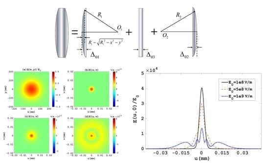
where ${\Delta }_0$ is the maximum thickness of lens, $\Delta (x,y)$ is the thickness function of lens and $n(x,y)$ is the space-dependent refraction index of lens at position $(x,y)$. If the lens is considered as the superposition of three parts, as shown in Figure 1, the total thickness function can be written as

$$\Delta (x,y)={\Delta }_1(x,y)+{\Delta }_2(x,y)+{\Delta }_3(x,y),$$

(6)

which is the sum of three individual thickness functions. According to the geometric relationship illustrated in Figure 1, the thickness function ${\Delta }_1(x,y)$ of the left part is given by

$${\Delta }_1(x,y)={\Delta }_{01}-(R_1-\sqrt{R_1{}^2-x^2-y^2})={\Delta }_{01}-R_1(1-\sqrt{1-\frac{x^2+y^2}{R_1{}^2}}).$$

(7)

where $R_1$ is the radius of the left spherical surface of optical lens and $R_1=\infty$ for a planar lens surface. Similarly, the right part has a thickness function given by

$${\Delta }_2(x,y)={\Delta }_{02}-(R_2-\sqrt{R_2{}^2-x^2-y^2})={\Delta }_{02}+R_2(1-\sqrt{1-\frac{x^2+y^2}{R_2{}^2}}).$$

(8)

where $R_2$ is the radius of the right spherical surface of optical lens and $R_2=\infty$ for a planar lens surface. In this work, the values of $x$ and $y$ are considered relatively small as compared to the radii of the two spherical surfaces of lens, so that the following approximations hold true with sufficient accuracy [15],

$$\sqrt{1-\frac{x^2+y^2}{R_i{}^2}}\approx 1-\frac{x^2+y^2}{2R_i{}^2},$$

(9)

for $i=1,2$, respectively. The central component part is a flat glass with constant thickness, ${\Delta }_3(x,y)={\Delta }_{03}$. Finally, we get the total thickness function given by

$$\Delta (x,y)={\Delta }_0-{\frac{x^2+y}{2}}^2(\frac{1}{R_1}-\frac{1}{R_2}),$$

(10)

where ${\Delta }_0={\Delta }_{01}+{\Delta }_{02}+{\Delta }_{03}$. It is noted that the nominal focal length of optical lens, $f_0$, is defined by

$$\frac{1}{f_0}\equiv (n_0-1)(\frac{1}{R_1}-\frac{1}{R_2}).$$

(11)

Then, by combining Equations (4), (10), and (11), we obtain the transfer function of lens

$$t(x,y)=\exp [\mathrm{j}\varphi (x,y)]=\exp \left[\mathrm{j}k{n}_0{\Delta }_0\right]\exp \left[\mathrm{j}k\beta (x,y){\left|E(x,y)\right|}^2\right]\exp \left[-\frac{\mathrm{j}k}{2f_0}(x^2+y^2)\right],$$

(12)

where the spatial function $\beta (x,y)=\alpha [{\Delta }_0-\frac{x^2+y^2}{2f_0(n_0-1)}]$ is proportional to the parameter $\alpha$.

We further assume that the coordinates of the rear nominal focal plane of lens with $z=f_0$ are $(u,v)$, and use the Fresnel diffraction integral formula to calculate the focal spots formed by the optical lens. In fact, the field pattern of focal spots in the rear nominal focal plane is given by

$$E(u,v)=\frac{\exp [\mathrm{j}\frac{k}{2f_0}(u^2+v^2)]}{\mathrm{j}\lambda f_0}\times {\displaystyle \iint E(x,y)t(x,y)\exp \left[\frac{\mathrm{j}k}{2f_0}(x^2+y^2)\right]\exp [-\frac{\mathrm{j}2\pi }{\lambda f_0}(xu+yv)]}\mathrm{d}x\mathrm{d}y,$$

(13)

where $E(x,y)$ is the complex light field distribution of an incident laser beam in the front plane of the lens. On substituting Equation (12) into Equation (13), the quadratic phase factor within the integrand are canceled, and one obtains

$$\begin{array}{ll}E(u,v)& =\frac{\exp [\mathrm{j}\frac{k}{2f_0}(u^2+v^2)]}{\mathrm{j}\lambda f_0}\exp \left[\mathrm{j}k{n}_0{\Delta }_0\right]\\ & \times {\displaystyle \iint E(x,y)\exp \left[\mathrm{j}k\beta (x,y){\left|E(x,y)\right|}^2\right]\exp [-\frac{\mathrm{j}2\mathsf{\pi }}{\lambda f_0}(xu+yv)]}\mathrm{d}x\mathrm{d}y.\end{array}$$

(14)

Based on the light field distribution in the nominal focal plane given by Equation (14), we can further calculate the light field distribution in several transverse planes adjacent to the nominal focal plane according to the angular spectrum algorithm. As a matter of fact, we can define the transfer function of angular spectrum diffraction as

$$H_{\mathrm{AS}}(f_x,f_y)=\exp \left(\mathrm{j}\frac{2\mathsf{\pi }\Delta z}{\lambda }\sqrt{1-{\lambda }^2(f_x^2+f_y^2})\right),$$

(15)

where $f_x$ and $f_y$ are the spatial frequency in the $x$ and $y$ directions, respectively. Then the laser transmission in free space from the transverse plane $U\left(x_0,y_0,z_0\right)$ to the transverse plane $U\left(x,y,z\right)$ with interval distance $\Delta z$ can be calculated by the formula of angular spectrum,

$$U(x,y,z)=F^{-1}\{F[U(x_0,y_0,z_0)]H_{\mathrm{AS}}(f_x,f_y)\},$$

(16)

where $F$ and $F^{-1}$ represent the two-dimensional Fourier transform and inverse Fourier transform, respectively [16,17]. Then the light field distribution of focal spots in the transverse plane of interest with the specified interval distance $\Delta z$ away from the nominal focal plane can be numerically calculated by applying the 2D-FFT and 2D-IFFT algorithms on Equation (16).

3. Calculation Method and Parameter Selection

The Fresnel diffraction integral formula given by Equation (14) is usually too difficult to be analytically calculated since the integrand may be complicated. Thus, the numerical methods are often applied. We can rewrite Equation (14) into the form of two-dimensional Fourier transform,

$$E(u,v)=\frac{\exp [\mathrm{j}\frac{k}{2f_0}(u^2+v^2)]}{\mathrm{j}\lambda f_0}\exp \left[\mathrm{j}k{n}_0{\Delta }_0\right]\times F{\left\{E(x,y)\exp \left[\mathrm{j}k\beta (x,y){\left|E(x,y)\right|}^2\right]\right\}|}_{f_x=\frac{u}{\lambda f_0},f_y=\frac{v}{\lambda f_0}}$$

(17)

To numerically calculate the double integral of two-dimensional Fourier transform in Equation (17), the efficient algorithm based on the two-dimensional fast Fourier transform (2D-FFT) is utilized. For this purpose, we first spatially discretize the front plane $(x,y)$ of optical lens, make the 2D-FFT manipulation, and then apply the variable substitutions $f_x=u/(\lambda f_0)$ and $f_y=v/(\lambda f_0)$ to obtain the light field distribution in the focal plane $(u,v)$. Assume that the sizes of computational domain in the front lens plane are $L_x\times L_y$, and the gird numbers of the two-dimensional discrete mesh are $N_x\times N_y$ with discrete grid sizes $\Delta x=L_x/N_x$ and $\Delta y=L_y/N_y$. Then, the discrete parameters in the spatial domain and the frequency domain satisfy the relationship

$$\begin{array}{l}\Delta f_x=\frac{1}{\Delta x{N}_x}=\frac{1}{L_x},\Delta u=\lambda f_0\Delta f_x=\frac{\lambda f_0}{L_x},\\ \Delta f_y=\frac{1}{\Delta y{N}_y}=\frac{1}{L_y},\Delta v=\lambda f_0\Delta f_y=\frac{\lambda f_0}{L_y}.\end{array}$$

It can be seen that the discrete grid sizes in the focal plane, $\Delta u$ and $\Delta v$, are determined by the sizes of computational domain, $L_x$ and $L_y$, rather than the grid numbers, $N_x$ and $N_y$.

In practice, the of computational sizes $L_x$ and $L_y$ are determined by two factors—the waist size of incident laser beam and the grid fineness of focal plane. In order to avoid the aliasing errors in the 2D-FFT manipulation, it is necessary to ensure that the spectral components of the original function satisfy the Nyquist sampling conditions [18,19]. That is, the highest spectral component of

$$U(x,y)=E(x,y)\exp \left[\mathrm{j}k\beta (x,y){\left|E(x,y)\right|}^2\right]$$

(18)

should satisfy the conditions, $f_x{}_{\max }\le 1/(2\Delta x)$ and $f_y{}_{\max }\le 1/(2\Delta y)$. The requirements can be utilized to choose the proper grid sizes, $\Delta x$ and $\Delta y$. Then the grid numbers, $N_x$ and $N_y$, can be determined. For the incidence of an axisymmetric laser beam, the square computational domain with square discrete grids is set, so that $L_x=L_y=L$ and $N_x=N_y=N$.

In the following calculations, the nominal focal length and thickness of the focusing lens made by fused silica glass are assumed to be $f_0=2.2\mathrm{m}$ and ${\Delta }_0=0.01\mathrm{m}$, respectively. The wavelength of incident laser beams is $\lambda =351\mathrm{nm}$ in vacuum, which are usually applied in large laser facilities for realizing ICF. At this wavelength, the linear portion of refractive index of fused silica glass is $n_0=1.4767$ [20], the nonlinear refractive-index coefficient of light intensity is $\gamma =3.0\times {10}^{-16}$ cm²/W [21], and the nonlinear refractive-index coefficient of squared electric-field magnitude is $\alpha ={\epsilon }_{0}c{n}_0\gamma /2\approx 5.3\times {10}^{-23}{\mathrm{m}}^2{/\mathrm{V}}^2$. Moreover, the loss coefficient of fused silica is commonly between $8\times {10}^{-6}$ and $2\times {10}^{-5}$, depending on the purity of material. Thus, the absorption effect and loss of optical lens is ignored in this work.

In this work, three classical types of incident laser beams are considered. In most cases, a laser emits light in the form of a laser beam often close to a fundamental Gaussian beam, where the transverse profile of the optical intensity of the beam can be described with a Gaussian function and the variation of beam size can be very small for beams with large width. Thus, the first type is the fundamental Gaussian beam, whose electric field is given by

$$E(x,y,z)=E_0\frac{w_0}{w(z)}\exp \left(-\frac{x^2+y^2}{w{(z)}^2}\right)\exp \left[-\frac{\mathrm{i}k(x^2+y^2)}{2R(z)}-\mathrm{i}kz+\mathrm{i}\phi (z)\right],$$

(19)

where $E_0$ is the maximum field amplitude at the center of beam waist, $w_0$ is the radius of beam waist, $z_{\mathrm{R}}=\mathsf{\pi }{w}_0^2/\lambda$ is the Rayleigh length, $w\left(z\right)=w_0\sqrt{1+{\left(z/z_{\mathrm{R}}\right)}^2}$ is the beam radius at z, $R\left(z\right)=z+z_{\mathrm{R}}^2/z$ is the radius of curvature of the beam’s wavefront at $z$, and $\phi (z)=\arctan (z/z_{\mathrm{R}})$ is the Gouy phase shift. Therefore, we can substitute Equation (19) into Equation (17) to calculate the light field distribution of focal spots in the nominal focal plane of lens.

The second type are the Hermite-Gaussian beams. A Hermite-Gaussian beam is one of the higher-order solutions of the paraxial Helmholtz equation in Cartesian coordinate system. The expression of light field for the $(m,n)$th order Hermite-Gaussian laser beam is written as

$$\begin{array}{c}E(x,y,z)\text{}=E_0\frac{w_0}{w(z)}{H}_m\text{}\left(\frac{\sqrt{2}x}{w(z)}\right)\text{}{H}_n\text{}\left(\frac{\sqrt{2}y}{w(z)}\right)\exp \left(-\frac{x^2+y^2}{w^2(z)}\right)\times \\ \exp \left(-\mathrm{i}\frac{k(x^2+y^2)}{2R(z)}\right)\exp \left(\mathrm{i}{\phi }_{mn}(z)\right)\end{array}$$

(20)

where ${\phi }_{mn}(z)=(m+n+1){\tan }^{-1}(z/z_{\mathrm{R}})$ is the Gouy phase shift for the Hermite-Gaussian beams, $H_m(\cdot )$ and $H_n(\cdot )$ are the $m$th and $n$th Hermite polynomials [16]. It should be noticed that the Hermite-Gaussian beams degenerate to the fundamental Gaussian beam when $m=n=0$.

The third type are the Laguerre-Gaussian beams. A Laguerre-Gaussian beam is one of the high-order solutions of the paraxial Helmholtz equation in cylindrical coordinate system. The light field of the $(p,l)$th order Laguerre-Gaussian beam is given by

$$E_{lp}(r,\varphi ,z)=E_0\frac{w_0}{w(z)}{\left(\frac{\sqrt{2}r}{w(z)}\right)}^{\left|l\right|}{L}_p^{\left|l\right|}\text{}\left(\frac{2r^2}{w^2(z)}\right)\exp \left[-\mathrm{i}\left(\frac{k{r}^2}{2q(z)}+kz+l\varphi -{\phi }_{pl}(z)\right)\right],$$

(21)

where ${\phi }_{pl}(z)=(2p+\left|l\right|+1)ta{n}^{-1}(z/z_R)$ is the Gouy phase shift, and $L_p^l(·)$ is the associated Laguerre polynomial. A Laguerre-Gaussian beam of ${\mathrm{LG}}_p^l$ mode is specified by two mode indices, the angular mode index $l(l=0,\pm 1,\pm 2,\dots )$ and the transverse radial mode index $p(p=0,1,2,\dots )$. When $p=l=0$, the Laguerre-Gaussian beams degenerate to the fundamental Gaussian beam. When the angular mode index $l$ is greater than zero, the light field has an azimuthal phase change of $2\mathsf{\pi }l$, which results in a phase singularity in the field and a node in the intensity at the center of the beam. Thus, the laser beams propagating in Laguerre-Gaussian modes may have orbital angular momentum and multiply connected topology.

4. Results and Discussions

4.1. High-Intensity Fundamental Gaussian Beam

The normalized cross-sectional light field distribution of a fundamental Gaussian beam, $E(x,y)/E_0$, on the waist plane with waist radius $w_0=100\mathrm{mm}$ is depicted in Figure 2a. It can be seen from Figure 2a that the radius of the circle where the magnitude of light field drops to 1/e of the central maximum value is 99.61 mm. Three different levels of light field intensities of incident laser beams with $E_0=1\times {10}^8\mathrm{V}/\mathrm{m}$, $5\times {10}^8\mathrm{V}/\mathrm{m}$ and $1\times {10}^9\mathrm{V}/\mathrm{m}$ are applied, which are below, near and above the maximum damage threshold of fused silica, $40{\mathrm{GW}/\mathrm{cm}}^2$ [22]. The different field patterns of focal spots in the nominal focal plane of lens are shown in Figure 2c,d corresponding to the above three cases, respectively. It can be seen from Equation (3) that the different changes in refractive index for different levels of light intensities result in the different patterns of focal spots. For the case of incident laser beam with $E_0=1\times {10}^8\mathrm{V}/\mathrm{m}$ as shown in Figure 2b, the radius of focal spot on which the electric field magnitude drop to 1/e of the central maximum intensity is 2.4 µm. Further comparative study shows that the shape and radius of focal spot nearly do not change when $E_0<1\times {10}^8\mathrm{V}/\mathrm{m}$, in which situation the impact of Kerr effect can be ignored. For the case with $E_0=5\times {10}^8\mathrm{V}/\mathrm{m}$, the shape of focal spot is different from that of the former case, but the Gaussian-type distribution still holds, and the radius of focal spot with 1/e of field magnitude increases to 2.9 µm. However, as for the case with $E_0=1\times {10}^9\mathrm{V}/\mathrm{m}$, it can be seen that the Kerr effect has significant influence on the focusing performance of optical lens. It is noted that there are two distinct annular light rings appearing around the center focus. By measuring the obtained result, the radii of the two annular light rings are 3.9 µm and 11.9 µm, respectively.

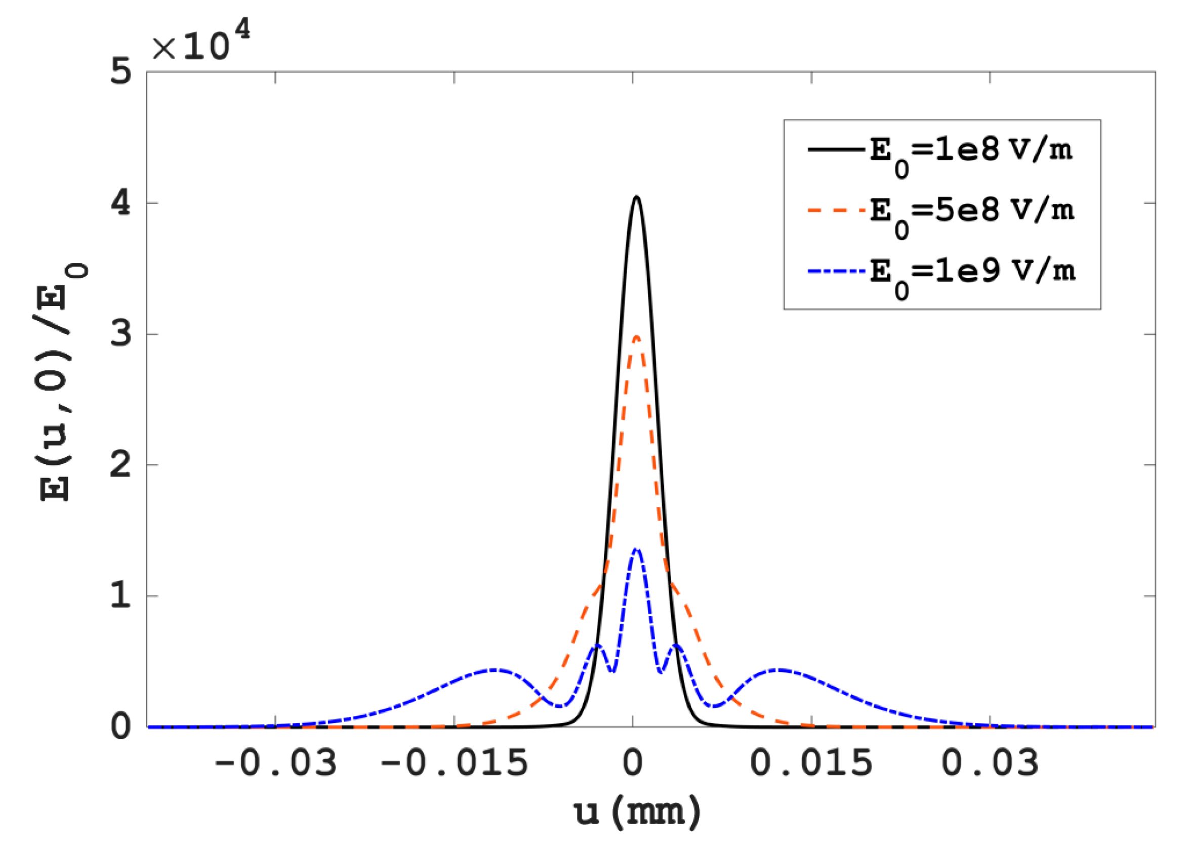
In order to further evaluate the impact of Kerr effect on the focusing performance of lens for the Gaussian beams with three different intensities, the light field intensities of focal spots are normalized by $E_0$. The radial distributions of light field intensities of focal spots are plotted in Figure 3. It can be seen that as the intensity of the incident laser beams increases, the relative light field intensity of the central focus becomes lower. The light energy becomes divergent and annular light rings gradually formed. For example, the relative light field intensity of central focus in the case with the highest intensity $E_0=1\times {10}^9\mathrm{V}/\mathrm{m}$ is approximately one-third of that of the first case with the lowest intensity $E_0=1\times {10}^8\mathrm{V}/\mathrm{m}$. The obtained results imply that, in order to avoid the influence of the Kerr effect on the focusing performance of lens, the intensity of the incident laser beam must be less than a certain value, which is relevant to the type of material used for lens fabrication. For the fused silica, the threshold of field strength is approximately $E_0=1\times {10}^8\mathrm{V}/\mathrm{m}$.

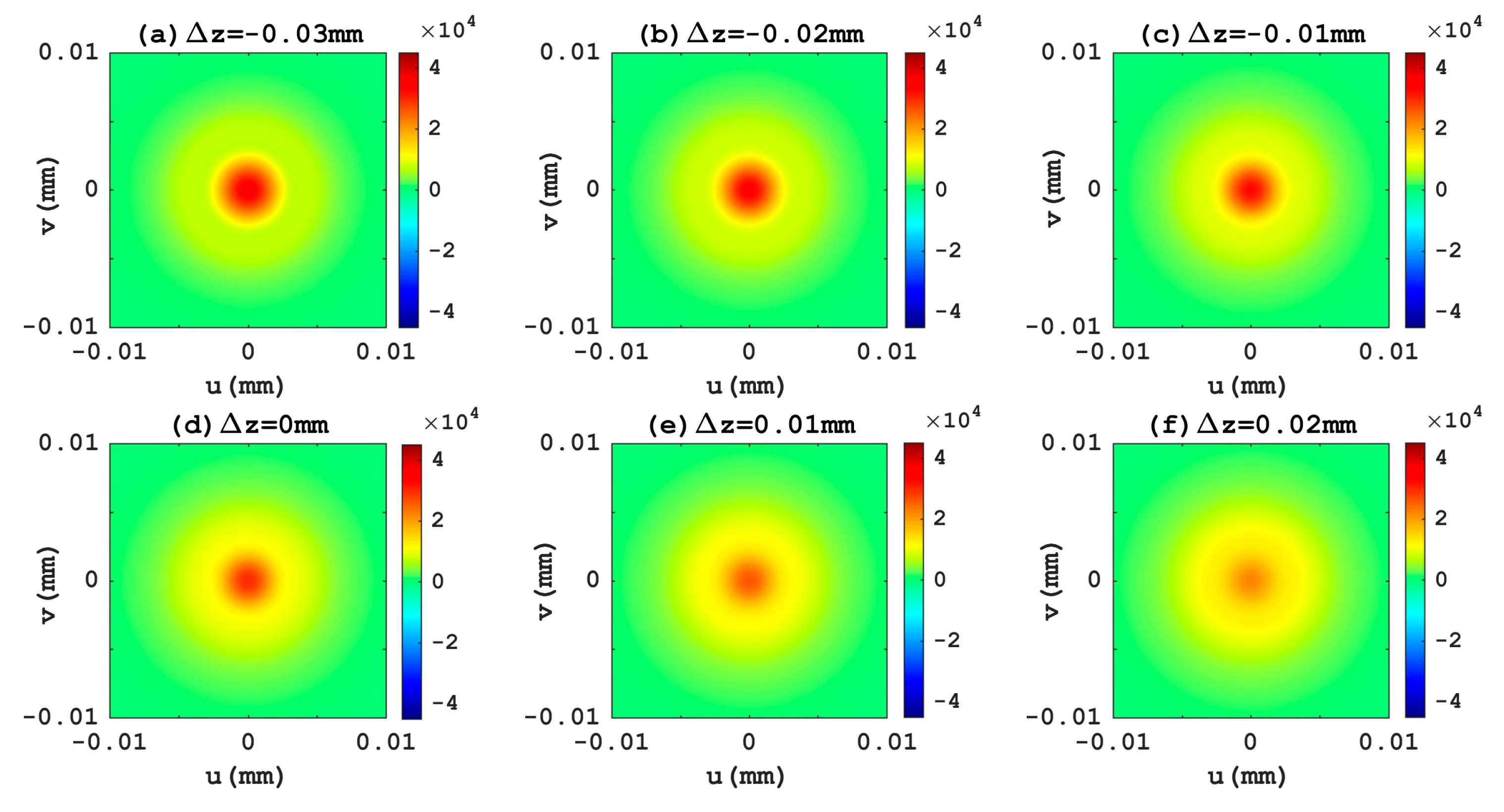
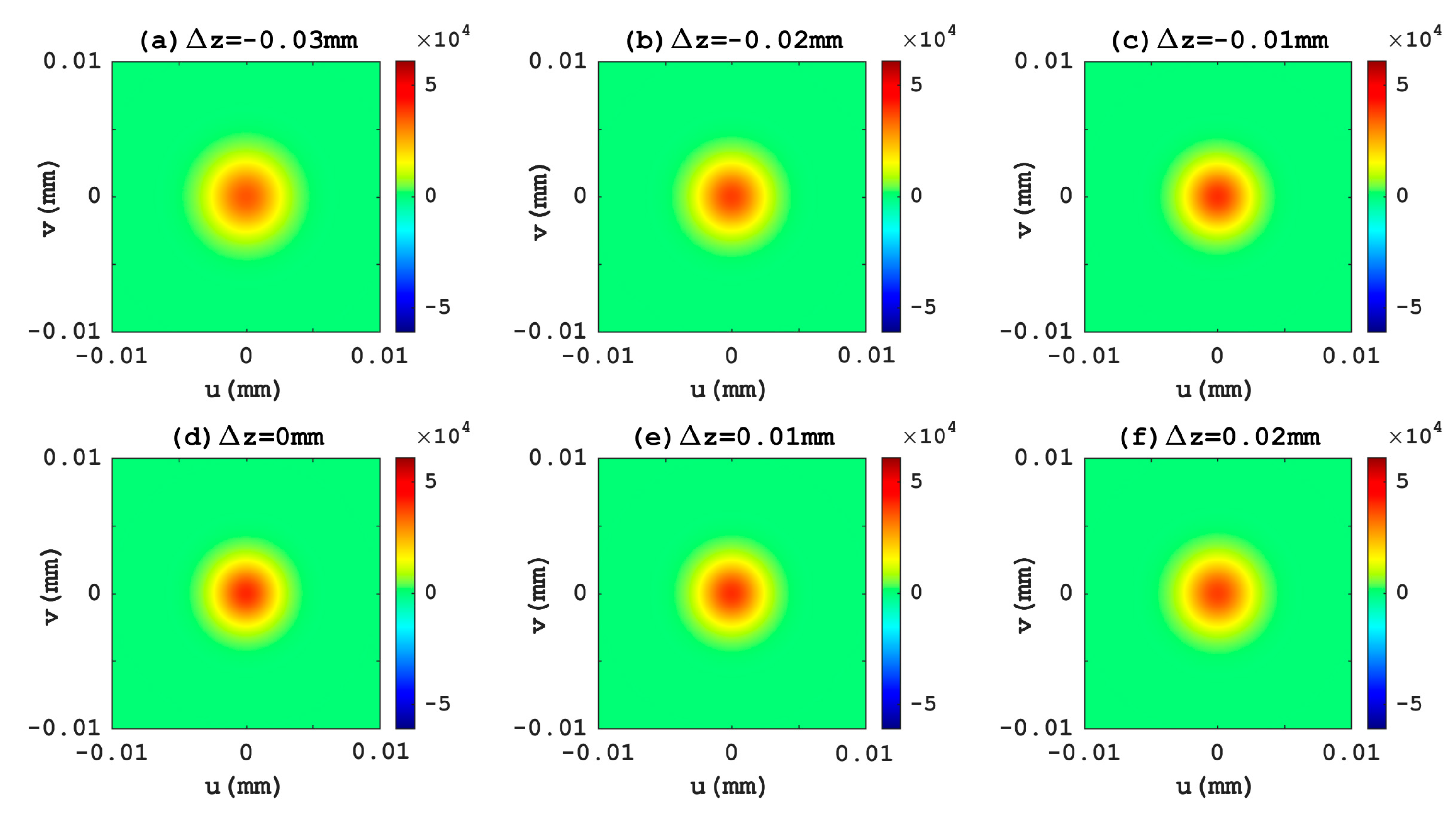
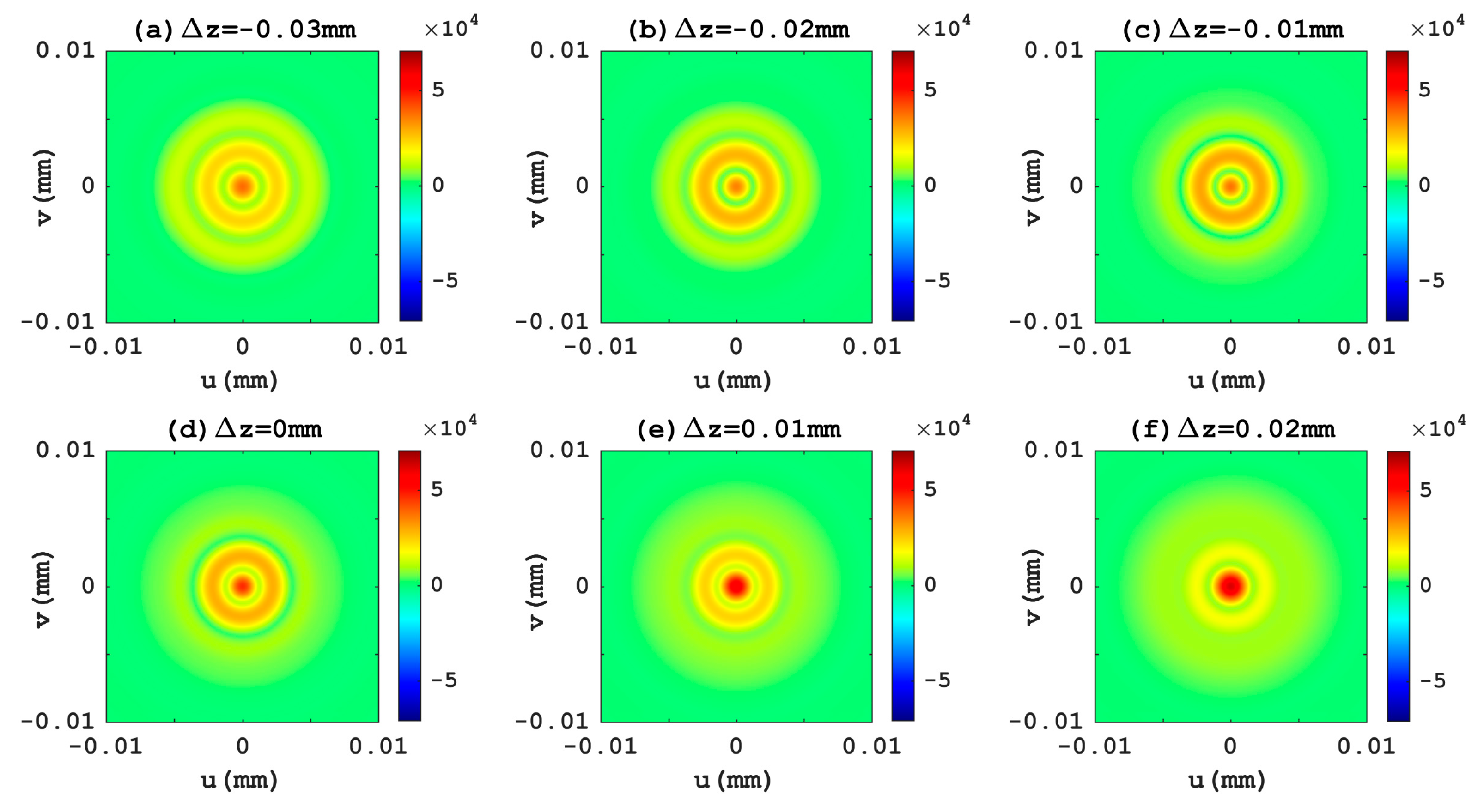
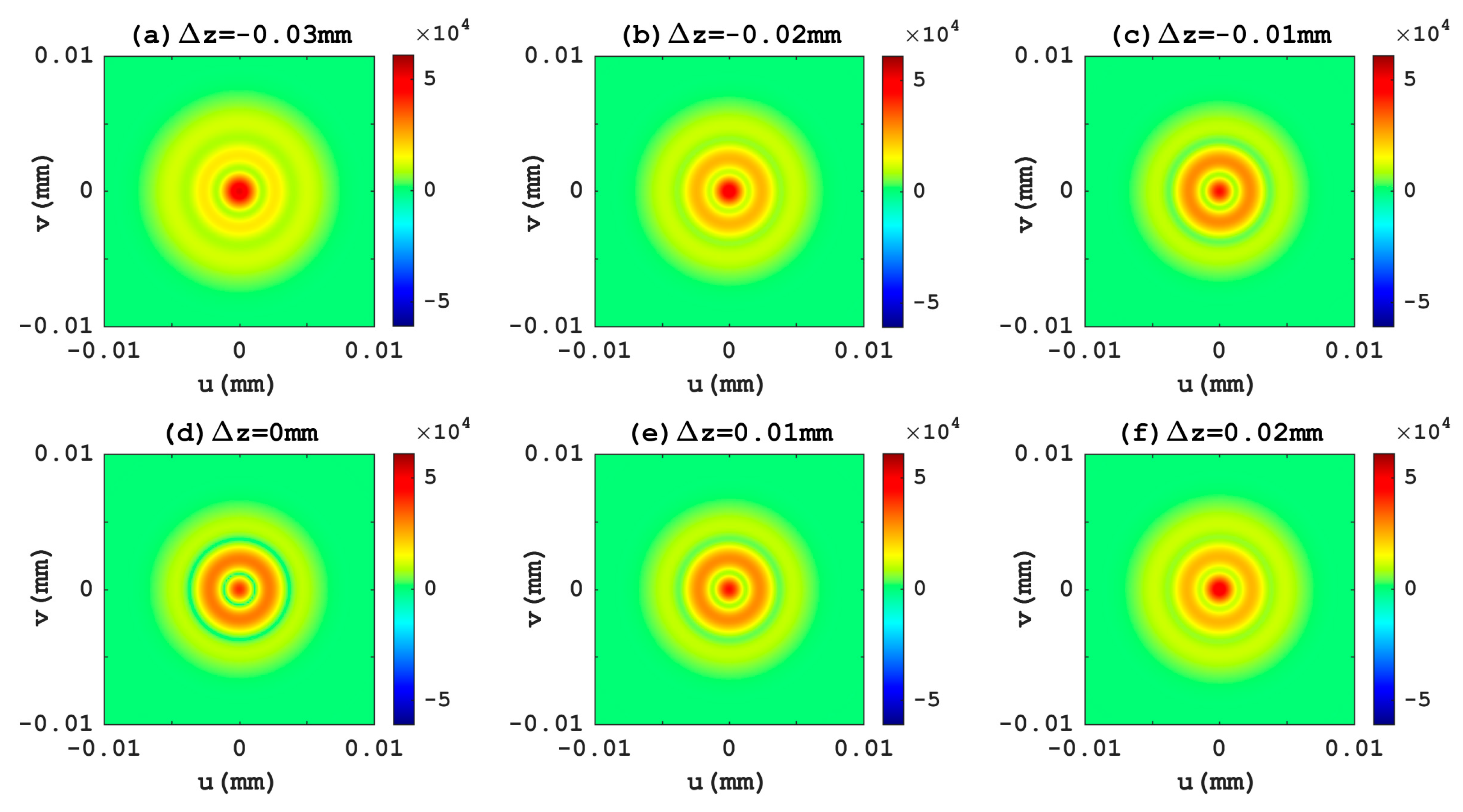
Beside the nominal focal plane, the light field distributions in several transverse planes adjacent to the nominal focal plane are calculated using the angular spectrum algorithm in order to acquire more information about the focusing performance of optical lens influenced by the Kerr effect. For the light field intensity of incident laser beam, $E_0=5\times {10}^8\mathrm{V}/\mathrm{m}$, the corresponding patterns of focal spots in the planes, which are of 0.03 mm, 0.03 mm and 0.01 mm left to the nominal focal plane are shown in Figure 4a–c, respectively. We can see that the Kerr effect makes the actual focal plane nearer to the optical lens and the effective focal length become shorter. By further calculation, we find that the actual focal spot is about 0.02 mm in front of the nominal focal plane. Figure 4e,f show the light field distributions of focal spots in the transverse planes right to the nominal focal plane by 0.01 mm and 0.02 mm, respectively. Figure 4d shows the same of light field distribution of focal spots in the nominal focal plane as that shown in Figure 2c for the convenience of comparison. We find that the focal spots gradually diverge with the increment of interval distance $\Delta z$. In Figure 5, we also present the patterns of focal spots in the six planes the same as those specified in Figure 4 when the Kerr effect is not taken into consideration by setting the coefficient $\alpha =0$. It can be seen that the sizes and patterns of the focal spots are nearly the same in the six planes. Thus, the Kerr effect of optical lens enhances the diffraction of focal spots.

4.2. High-Intensity Hermite-Gaussian Beam

As the second example, the incident beam is assumed to be the Hermite-Gaussian beam of ${\mathrm{HG}}_{11}$ mode. The normalized light field distributions of the incident ${\mathrm{HG}}_{11}$ laser beam in the lens plane is shown in Figure 6a with waist size $w_0=0.1\mathrm{m}$. Figure 6b–d show the different field patterns of focal spots in the nominal focal plane corresponding to three incident laser beams of different intensities with $E_0=1\times {10}^8\mathrm{V}/\mathrm{m}$, $5\times {10}^8\mathrm{V}/\mathrm{m}$ and $1\times {10}^9\mathrm{V}/\mathrm{m}$, respectively. Similarly, for the case with $E_0=1\times {10}^8\mathrm{V}/\mathrm{m}$, the pattern of focal spot shown in Figure 6b is similar to that of incident light field shown in Figure 6a, which indicates that the Kerr effect has little influence on the lens’s focusing performance when the light field intensity is smaller than $E_0=1\times {10}^8\mathrm{V}/\mathrm{m}$. However, for the case with $E_0=5\times {10}^8\mathrm{V}/\mathrm{m}$, it can be seen that the pattern of focal spot is significantly different from the former case. The pattern of focal spots changes from four spots into an array of spots. It is also noted that the closer to the periphery, the lower the intensity of spots. If we further increase the intensity of incident laser beam to $E_0=1\times {10}^9\mathrm{V}/\mathrm{m}$, the divergence of light energy become more apparent. Except for the central four focused spots, many light speckles are distributed on the entire calculation domain. Further calculation verifies that the increment of spatial sampling density and the increased number of discrete grids do not change the pattern of focal spots. Therefore, the speckles are correct results, but not due to under-sampling and aliasing phenomena in the numerical calculation implemented by the 2D-FFT algorithm.

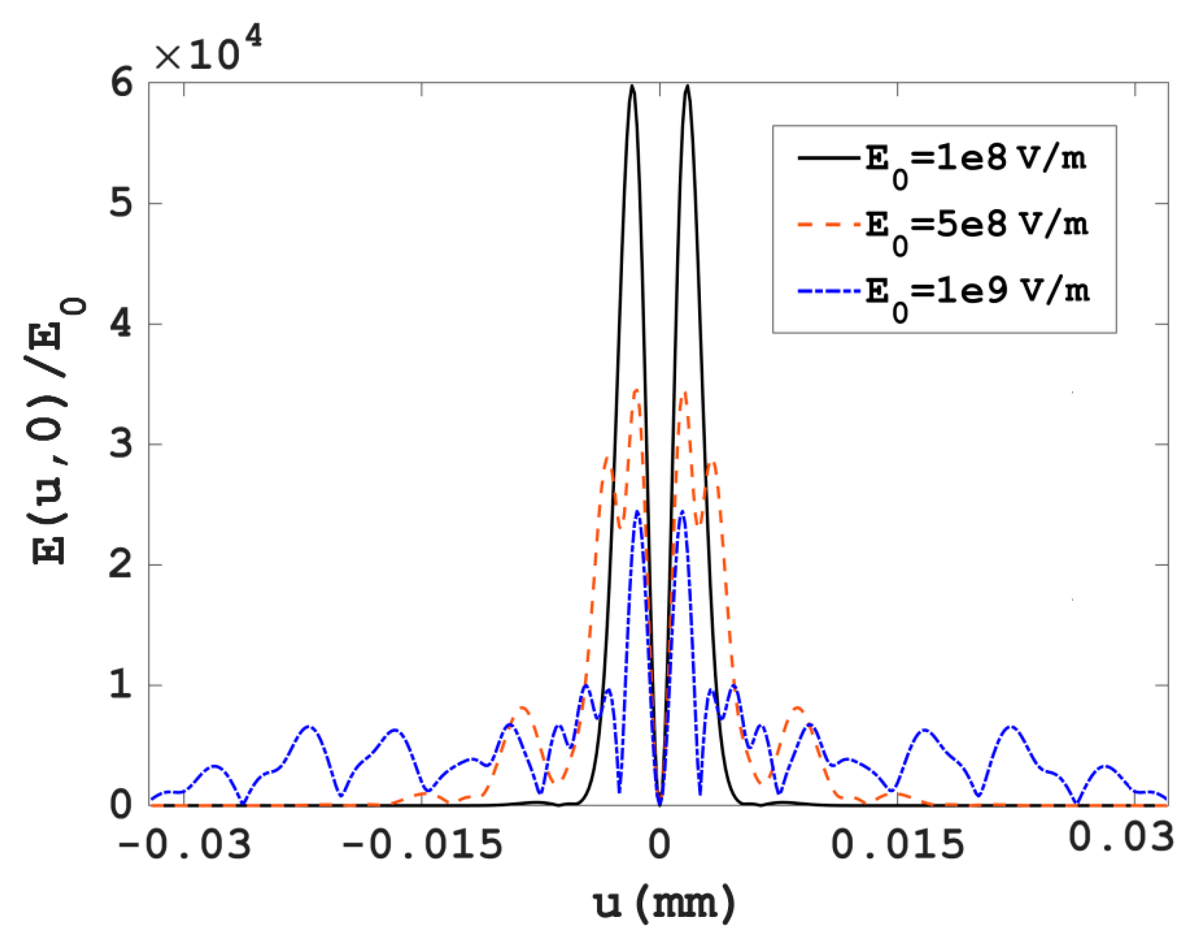
In order to fairly compare the field patterns of focal spots shown in Figure 6b–d for the three different intensities of incident laser beams, we first normalize the field intensities of focal spots by $E_0$ and the normalized light field distributions along the diagonal lines of computational domains are plotted in Figure 7. It can be seen that as the intensity of incident laser beam increases, the degree of divergence of focal spots is higher, and the intensity of the central focal spot becomes lower. In particular, for the case with $E_0=5\times {10}^8\mathrm{V}/\mathrm{m}$, the pattern of the four central focal spots are more complicated than the other two cases. It is found that the normalized light field intensity of the third case with $E_0=1\times {10}^9\mathrm{V}/\mathrm{m}$ is about 0.4 of that of the first case with $E_0=1\times {10}^8\mathrm{V}/\mathrm{m}$.

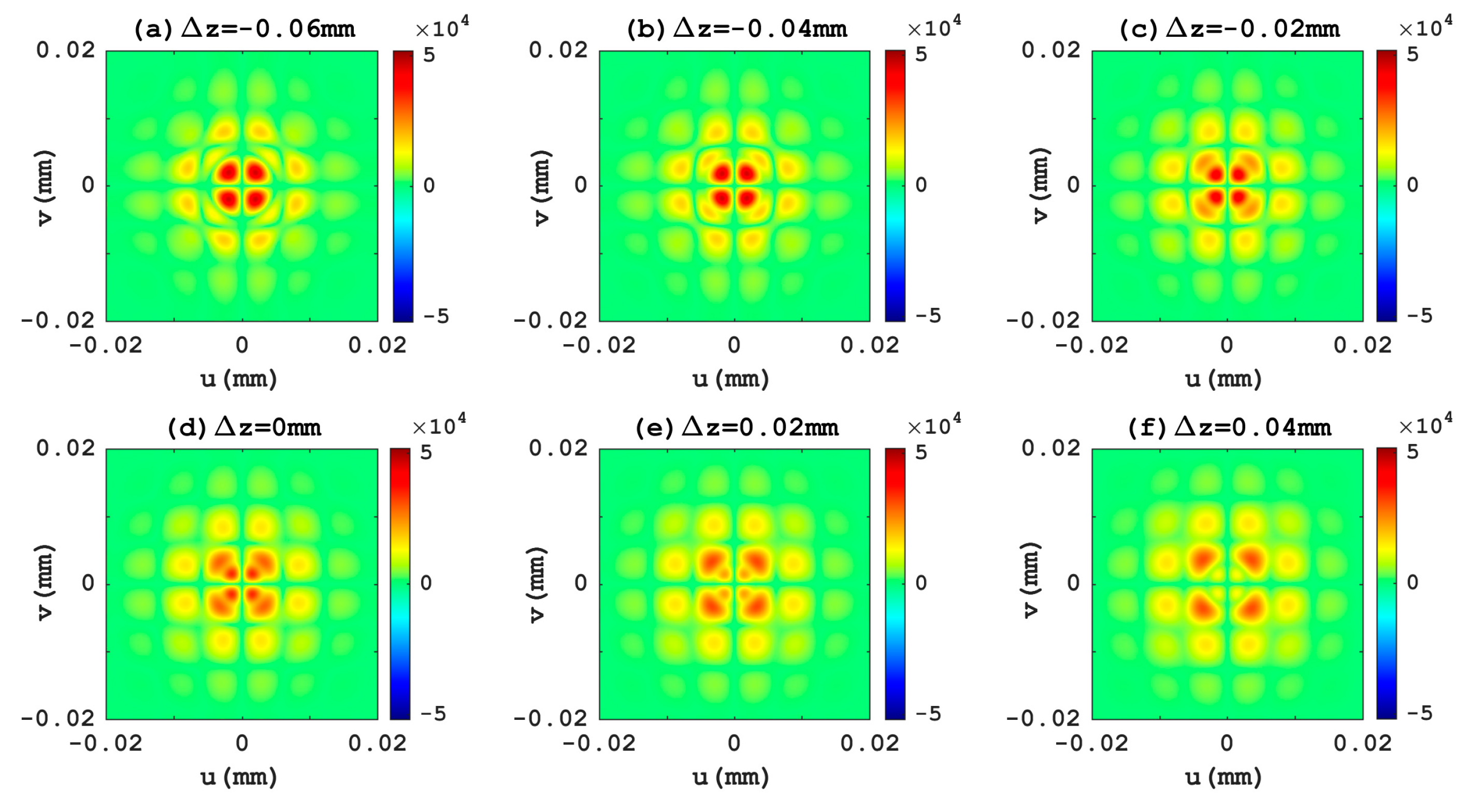
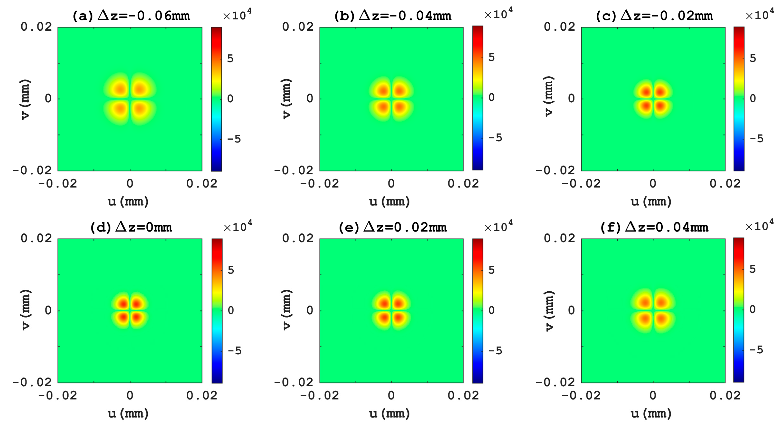
In order to evaluate the overall impact of Kerr effect on the focusing of Hermite-Gaussian beams, the field patterns of focal spots in the six specified planes are given in Figure 8a–f, which are of 0.06 mm, 0.04 mm, and 0.02 mm left to the nominal focal plane and 0 mm, 0.02 mm, and 0.04 mm right to the nominal focal plane for the ${\mathrm{HG}}_{11}$ laser beams with $E_0=5\times {10}^8\mathrm{V}/\mathrm{m}$. It can be seen that there are some weak speckles around the four central focusing spots and the actual focal plane of lens is left to the nominal focal plane if the Kerr effect is takes into consideration. We also find that the field patterns of focal spots gradually diverge with the increment of interval distance $\Delta z$. In Figure 9, we also show the field patterns of focal spots in the six planes without consideration of Kerr effect by setting the coefficient $\alpha =0$. It can be seen that the patterns of the focal spots are nearly the same in the six planes although a little enlarged in the first and last planes. Thus, the Kerr effect can affect the focusing performance of lens for the incidence of high-intensity Hermite-Gaussian beams.

4.3. High-Intensity Laguerre-Gaussian Beam

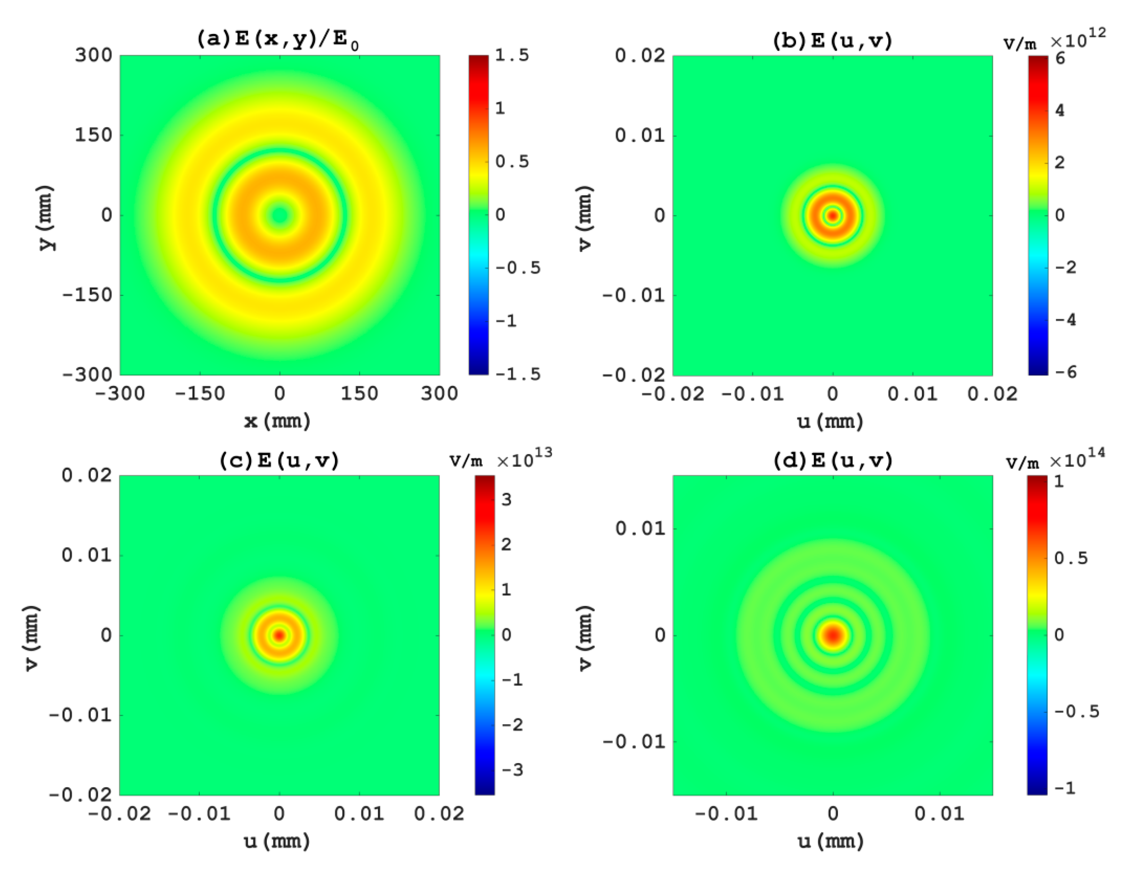
The last type of incident beams are the Laguerre-Gaussian beams. The field patterns of focal spots for Laguerre-Gaussian beams are different from the former two types of beams. Figure 10a is the normalized light field distribution of the incident Laguerre-Gaussian beam of ${\mathrm{LG}}_1^2$ mode with $w_0=0.1\mathrm{m}$. Figure 10b–d show the field patterns of focal spots in the nominal focal plane corresponding to three different light-field intensities, $E_0=1\times {10}^8\mathrm{V}/\mathrm{m}$, $5\times {10}^8\mathrm{V}/\mathrm{m}$ and $1\times {10}^9\mathrm{V}/\mathrm{m}$, respectively. It is found that the pattern of focal spots for the Laguerre-Gaussian beam with $E_0=1\times {10}^8\mathrm{V}/\mathrm{m}$ is quite different to those of fundamental Gaussian beam and Hermite-Gaussian beam. Except the two annual rings with different light field intensities, there is an exceptional focus at the center of rings. In the case shown in Figure 10c with $E_0=5\times {10}^8\mathrm{V}/\mathrm{m}$, the pattern of focal spots is similar to that of Figure 10b. However, the light-field intensities of the two rings become weakened and the light energy of focal spots further concentrates to the central focus. When the intensity of the incident laser beam rises to the level with $E_0=1\times {10}^9\mathrm{V}/\mathrm{m}$, the pattern is left with the dominant central focus and several negligible halos. The results demonstrate that when the light intensity of an incident Laguerre-Gauss beam reaches a certain level, the laser beam changes from a double-loop structure to a single high-intensity focus due to the nonlinear Kerr effect.

To further analysis the impact of the Kerr effect on the focusing performance of optical lens for different intensities of incident laser beams, the radial distributions of light field intensities of focal spots normalized by their corresponding levels of $E_0$ are plotted in Figure 11. It can be clearly seen that as the field intensity of incident laser beam increases, the light energy of outer rings is continuously concentrated to the central focus. For example, the relative light-field intensity of central focus in the case with the highest intensity $E_0=1\times {10}^9\mathrm{V}/\mathrm{m}$ is approximately twice of that of the first case with the lowest intensity $E_0=1\times {10}^8\mathrm{V}/\mathrm{m}$ and 1.7 of that of the median case with the medium intensity $E_0=5\times {10}^8\mathrm{V}/\mathrm{m}$. It is interesting to find that the incident LG beam can be focused into the central bright focus when the Kerr effect of lens is significant, which is quite different from the hollow structure of the incident LG beam with a node in the intensity at the center of beam.

In order to fully understand the influence of the Kerr effect on the focusing performance of lens for the case of the Laguerre-Gaussian beam (${\mathrm{LG}}_1^2$) with $E_0=5\times {10}^8\mathrm{V}/\mathrm{m}$, the field patterns of focal spots in the six planes adjacent to the nominal focal plane, which are of 0.03 mm, 0.02 mm, and 0.01 mm left to the nominal focal plane and 0 mm, 0.01 mm, and 0.02 mm right to the nominal focal plane, are depicted in Figure 12a−f, respectively. It can be clearly seen from Figure 12 that the central spot becomes brighter and larger and the field intensities of the surroundings rings become weakened when the plane is away from the lens. In Figure 13, we also show the field patterns of focal spots in the six planes without consideration of Kerr effect with the coefficient $\alpha =0$. It also can be found that the field patterns of focal spots shown in Figure 13 without Kerr effect are opposite to those shown in Figure 12 with the Kerr effect when the plane of interest is away from the nominal focal plane.

4.4. Impact of Lens Parameters

From the transfer function of lens given in Equation (12), the phase modulation or the focusing performance of lens is not only related to the light field intensity of incident beam $E_0$ and the value of nonlinear coefficient $\alpha$, but also to the parameters of lens, including the focal length $f_0$ and refractive index $n_0$. In view of this fact, we also studied the influence of focal length and refractive index of lens on the normalized field pattern of focal spots in the nominal focal plane for the three different incident laser beams of field intensity $E_0=5\times {10}^8\mathrm{V}/\mathrm{m}$ as shown in Figure 14. By comparing the results shown in Figure 14a–f, we can see that, for a shorter focal length of lens with $f_0=1\mathrm{m}$, the sizes of focal spots shrink proportionally and the patterns of focal spots change in comparison with the cases with $f_0=2\mathrm{m}$ under the same refractive index of lens $n_0=1.5$, especially for the case of Hermite-Gaussian beams. On the other hand, when we change the value of refractive index from $n_0=1.5$ to $n_0=1.7$, the results shown in Figure 14d−i illustrate that the refractive index of lens also can influence the field patterns of focal spots under the same focal length of lens $f_0=2\mathrm{m}$. Therefore, in practical application, the field patterns of focal spots should be calculated based on the specific laser beam and lens parameters of engineering problem.

5. Conclusions

In this work, the impact of the nonlinear Kerr effect on the focusing performance of an optical lens is studied by comparing the field patterns of focal spots for three types of incident high-intensity laser beams with different levels of light field intensities. Based on the theory of nonlinear optics and Fresnel diffraction integral formula, the transfer function of optical lens that takes the Kerr effect into consideration is derived for the incidence of high-intensity laser beams. The 2D-FFT algorithm was employed to reduce the computation resource for the focus of large incident laser beams, and the Kerr effect is considered by adding phase term proportional to the Kerr effect in order to get the light field distributions of focal spots in the nominal focal planes. The angular spectrum algorithm is utilized to calculate the field patterns of focal spots in the several transversal planes adjacent to the nominal focal plane for the three different types of incident laser beams. The obtained results show that the Kerr effect really affects the focusing performance of lens when the field intensity of incident laser lasers is above a threshold value. We find that the actual position of focal plane may be different from the position of nominal focal plane, depending on the type and light intensity of incident laser beams. The focal spots become larger and more divergent for the cases of fundamental Gaussian beams and Hermite-Gaussian beams due to the Kerr effect of the lens. On the contrary, unlike the other two types of laser beams, the field distribution of focal spots for the case of Laguerre-Gaussian beam becomes more concentrated with the increment of light intensity. Meanwhile, the parameters of lens, such as the focal length and refractive index, also can influence the field patterns of focal spots. The theory, algorithms and results presented in this work have potential applications in research fields such as the high-power laser physics and the design of focusing lens in the systems of large ICF laser facility.

References

- Hickstein, D.D.; Carlson, D.R.; Mundoor, H.; Khurgin, J.B.; Srinivasan, K.; Westly, D.; Kowligy, A.; Smalyukh, I.I.; Diddams, S.A.; Papp, S.B. Self-organized nonlinear gratings for ultrafast nanophotonics. Nat. Photonics 2019, 13, 494–499. [Google Scholar] [CrossRef]
- Lindl, J.; Landen, O.; Edwards, J.; Moses, E.; NIC Team. Review of the National Ignition Campaign 2009–2012. Phys. Plasmas 2014, 21. [Google Scholar] [CrossRef]
- Rudolph, W.; Diels, J.C. Ultrashort Laser Pulse Phenomena, 2nd ed.; Academic Press: Salt Lake City, UT, USA, 2006; pp. 314–322. ISBN 978-0-122-15493-5. [Google Scholar]
- Censor, D. Ray theoretic analysis of spatial and temporal self-focusing. Phys. Rev. A 1977, 16, 1673–1677. [Google Scholar] [CrossRef]
- Subbarao, D. Paraxial lens approximation and self-focusing theory. J. Opt. Soc. Am. B 2004, 21, 323–329. [Google Scholar] [CrossRef]
- Kasparian, J.; Solle, J.; Richard, M.; Wolf, J.-P. Ray-tracing simulation of ionization-free filamentation. Appl. Phys. B 2004, 79, 947–951. [Google Scholar] [CrossRef]
- Wei, J.; Yan, H. Laser beam induced nanoscale spot through nonlinear "thick" samples: A multi-layer thin lens self-focusing model. J. Appl. Phys. 2014, 116. [Google Scholar] [CrossRef] [Green Version]
- Lee, H.-H.; Chae, K.-M.; Yim, S.-Y.; Park, S.-H. Finite-difference time-domain analysis of self-focusing in a nonlinear Kerr film. Opt. Express 2004, 12, 2603–2609. [Google Scholar] [CrossRef] [PubMed]
- Godoy-Rubio, R.; Romero-Garcia, S.; Ortega-Monux, A.; Wanguemert-Perez, J.G. Nonlinear wide-angle beam propagation method using complex Jacobi iteration in the Fourier domain. J. Opt. Soc. Am. B 2011, 28, 2142–2148. [Google Scholar] [CrossRef]
- Delen, N.; Hooker, B. Verification and comparison of a fast Fourier transform-based full diffraction method for tilted and offset planes. Appl. Opt. 2001, 40, 3525–3531. [Google Scholar] [CrossRef] [PubMed]
- Mas, D.; Perez, J. Fast numerical calculation of Fresnel patterns in convergent systems. Opt. Commun. 2003, 227, 245–248. [Google Scholar] [CrossRef]
- Okada, N.; Shimobaba, T. Band-limited double-step Fresnel diffraction and its application to computer-generated holograms. Opt. Express 2013, 21, 9192–9197. [Google Scholar] [CrossRef] [PubMed]
- Matsushima, K.; Shimobaba, T. Band-Limited Angular Spectrum Method for Numerical Simulation of Free-Space Propagation in Far and Near Fields. Opt. Express 2009, 17, 19662–19673. [Google Scholar] [CrossRef] [PubMed] [Green Version]
- Shen, Y.S. The Principle of Nonlinear Optics, 1st ed.; Wiley: New York, NY, USA, 1984; pp. 303–312. ISBN 978-0-471-43080-3. [Google Scholar]
- Goodman, J.W. Introduction to Fourier Optics, 2nd ed.; Roberts and Company Publishers: New York, NY, USA, 1996; pp. 63–82. [Google Scholar]
- Klein, M.V. Optics, 2nd ed.; Wiley: New York, NY, USA, 1986; ISBN 978-0-471-87297-9. [Google Scholar]
- Voelz, D.G.; Roggeman, M.C. Digital simulation of scalar optical diffraction: Revisiting chirp function sampling criteria and consequences. Appl. Opt. 2009, 48, 6132–6142. [Google Scholar] [CrossRef] [PubMed]
- Paulson, D.A.; Wu, C.S.; Davis, C.C. Randomized spectral sampling for efficient simulation of laser propagation through optical turbulence. J. Opt. Soc. Am. B 2019, 36, 3249–3262. [Google Scholar] [CrossRef] [Green Version]
- Spence, D.J.; Hooker, S.M. Simulations of the propagation of high-intensity laser pulses in discharge-ablated capillary waveguides. J. Opt. Soc. Am. B 2000, 17, 1565–1570. [Google Scholar] [CrossRef]
- Lang, M.L.; Wolfe, W.L. Optical constants of fused silica and sapphire from 0.3 to 25 µm. Appl. Opt. 1983, 22, 1267–1268. [Google Scholar] [CrossRef] [PubMed]
- Kim, K.S.; Stolen, R.H.; Reed, W.A.; Quoi, K.W. Measurement of the nonlinear index of silica-core and dispersion-shifted fibers. Opt. Lett. 1994, 19, 257–259. [Google Scholar] [CrossRef]
- Said, A.A.; Xia, T.; Dogariu, A.; Hagan, D.J.; Soileau, M.J.; Van Stryland, E.W.; Mohebi, M. Measurement of the optical damage threshold in fused quartz. Appl. Opt. 1995, 34, 3374–3376. [Google Scholar] [CrossRef] [Green Version]
Figure 1.
The three component parts of an optical lens and their structure parameters.
Figure 2.
(a) The normalized cross-sectional light field distribution of incident basic Gaussian beam in the lens plane; The field patterns of focal spots in the nominal focal plane corresponding to the incident Gaussian beams with three different light field intensities: (b) , (c) , and (d) .
Figure 3.
The radial distributions of normalized light field intensities of focal spots in the nominal focal plane for the incident fundamental Gaussian beams with three different light field intensities, , and , respectively.
Figure 4.
The different field patterns of focal spots in the six planes, which are of (a) 0.03 mm, (b) 0.02 mm, and (c) 0.01 mm left to the nominal focal plane, respectively, and (d) 0 mm, (e) 0.01 mm, and (f) 0.02 mm right to the nominal focal plane for the incident fundamental Gaussian beam with field intensity .
Figure 5.
The different patterns of focal spots in the six planes the same as those specified in Figure 4 for the incident fundamental Gaussian beam with field intensity , where the Kerr effect of optical lens is not taken into consideration by setting the nonlinear coefficient .
Figure 6.
(a) The normalized cross-sectional light field distribution of incident Hermite-Gaussian beam () in the lens plane. The three field patterns of focal spots corresponding to the incident Hermite-Gaussian beams with three different light field intensities: (b) , (c) , and (d) .
Figure 7.
The normalized light field intensities of focal spots in the nominal focal plane along the diagonal lines of computational domains for the incident Hermite-Gaussian beams of mode with three different light field intensities, , and , respectively.
Figure 8.
The different patterns of focal spots in the six planes, which are of (a) 0.06 mm, (b) 0.04 mm and (c) 0.02 mm left to the nominal focal plane, respectively, and (d) 0 mm, (e) 0.02 mm and (f) 0.04 mm right to the nominal focal plane for the incident Hermite-Gaussian beam with field intensity .
Figure 9.
The different patterns of focal spots in the six planes the same as those specified in Figure 8 for the incident Hermite-Gaussian beam with field intensity , where the Kerr effect of optical lens is not taken into consideration by setting the nonlinear coefficient .
Figure 10.
(a) The normalized cross-sectional light field distribution of the incident Laguerre-Gaussian beam () in the lens plane. The three field patterns of focal spots correspond to the incident Laguerre-Gaussian beams with different light field intensities: (b) , (c) , and (d) .
Figure 11.
The radial distributions of the normalized light field intensities of focal spots in the nominal focal plane for incident Laguerre-Gaussian beams of mode with three different light field intensities, , and , respectively.
Figure 12.
The different patterns of focal spots in the six planes, which are of (a) 0.03 mm, (b) 0.02 mm, and (c) 0.01 mm left to the nominal focal plane, respectively, and (d) 0 mm, (e) 0.01 mm, and (f) 0.02 mm right to the nominal focal plane for the incident Laguerre-Gaussian beam with field intensity .
Figure 13.
The different field patterns of focal spots in the six planes the same as those specified in Figure 12 for the incident Laguerre-Gaussian beam with field intensity , where the Kerr effect of optical lens is not taken into consideration by setting the nonlinear coefficient .
Figure 14.
The influence of different focal lengths and refractive indices of lens on the patterns of focal spots in the nominal focal plane for the three different incident laser beams of field intensity , the fundamental Gaussian beam, beam, and beam from left to right, where the lens parameters are (a–c) , ; (d–f) , ; (g–i) , , respectively.
© 2020 by the authors. Licensee MDPI, Basel, Switzerland. This article is an open access article distributed under the terms and conditions of the Creative Commons Attribution (CC BY) license (http://creativecommons.org/licenses/by/4.0/).
Share and Cite
MDPI and ACS Style
Yu, B.; Lin, Z.; Chen, X.; Qiu, W.; Pu, J. Impact of Nonlinear Kerr Effect on the Focusing Performance of Optical Lens with High-Intensity Laser Incidence. Appl. Sci. 2020, 10, 1945. https://doi.org/10.3390/app10061945
AMA Style
Yu B, Lin Z, Chen X, Qiu W, Pu J. Impact of Nonlinear Kerr Effect on the Focusing Performance of Optical Lens with High-Intensity Laser Incidence. Applied Sciences. 2020; 10(6):1945. https://doi.org/10.3390/app10061945
Chicago/Turabian StyleYu, Bosong, Zhili Lin, Xudong Chen, Weibin Qiu, and Jixiong Pu. 2020. "Impact of Nonlinear Kerr Effect on the Focusing Performance of Optical Lens with High-Intensity Laser Incidence" Applied Sciences 10, no. 6: 1945. https://doi.org/10.3390/app10061945
Note that from the first issue of 2016, this journal uses article numbers instead of page numbers. See further details here.