
High-Resolution Mapping and Assessment of Salt-Affectedness on Arable Lands by the Combination of Ensemble Learning and Multivariate Geostatistics

 , , ,
, , ,  , , , , and
Abstract
:1. Introduction
2. Materials and Methods
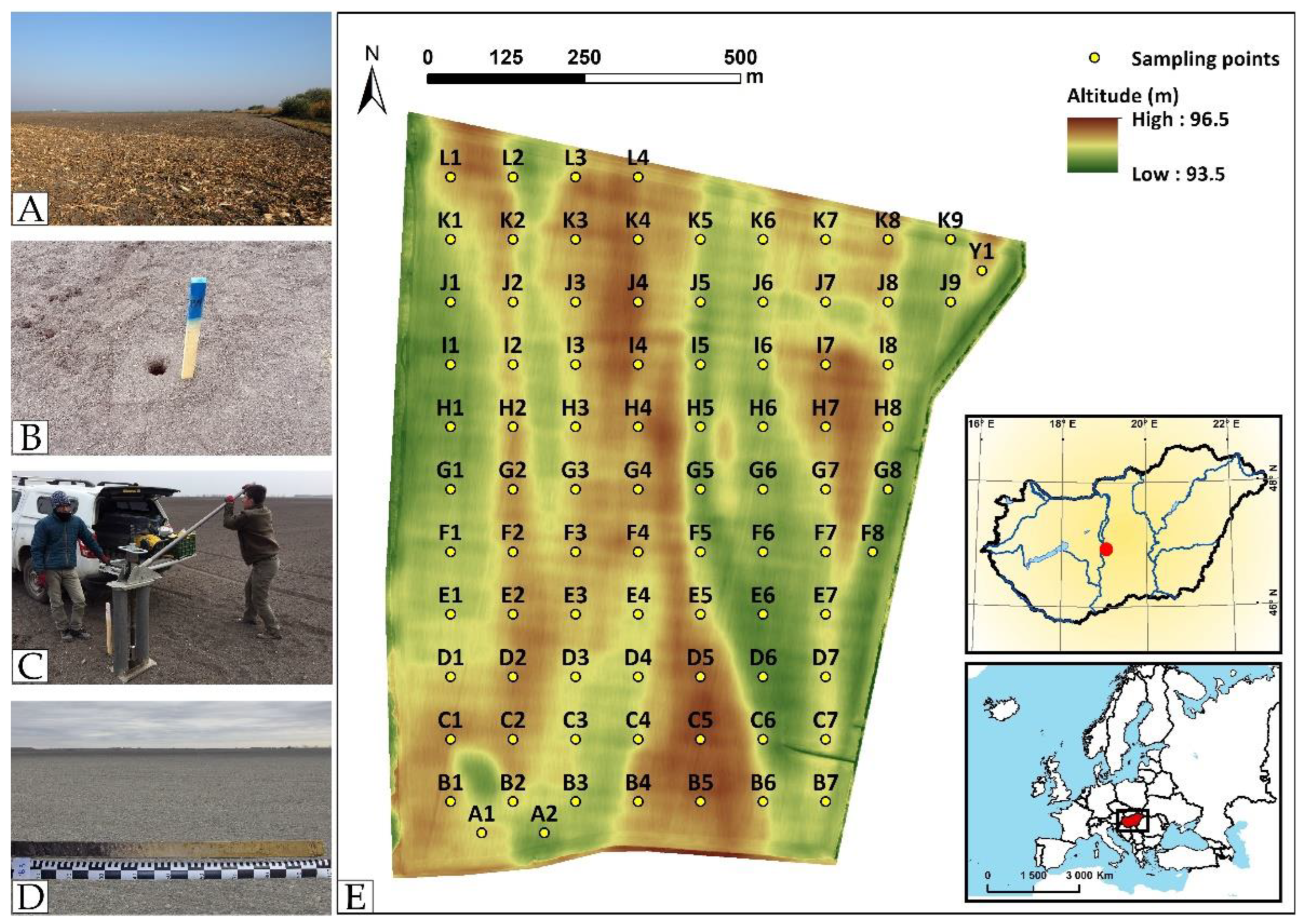
2.1. Study Site
2.2. Field Survey and Laboratory Analysis
2.3. Environmental Covariates
2.4. Spatial Modelling and Predictive Mapping
2.4.1. Ensemble Modelling for the Deterministic Component
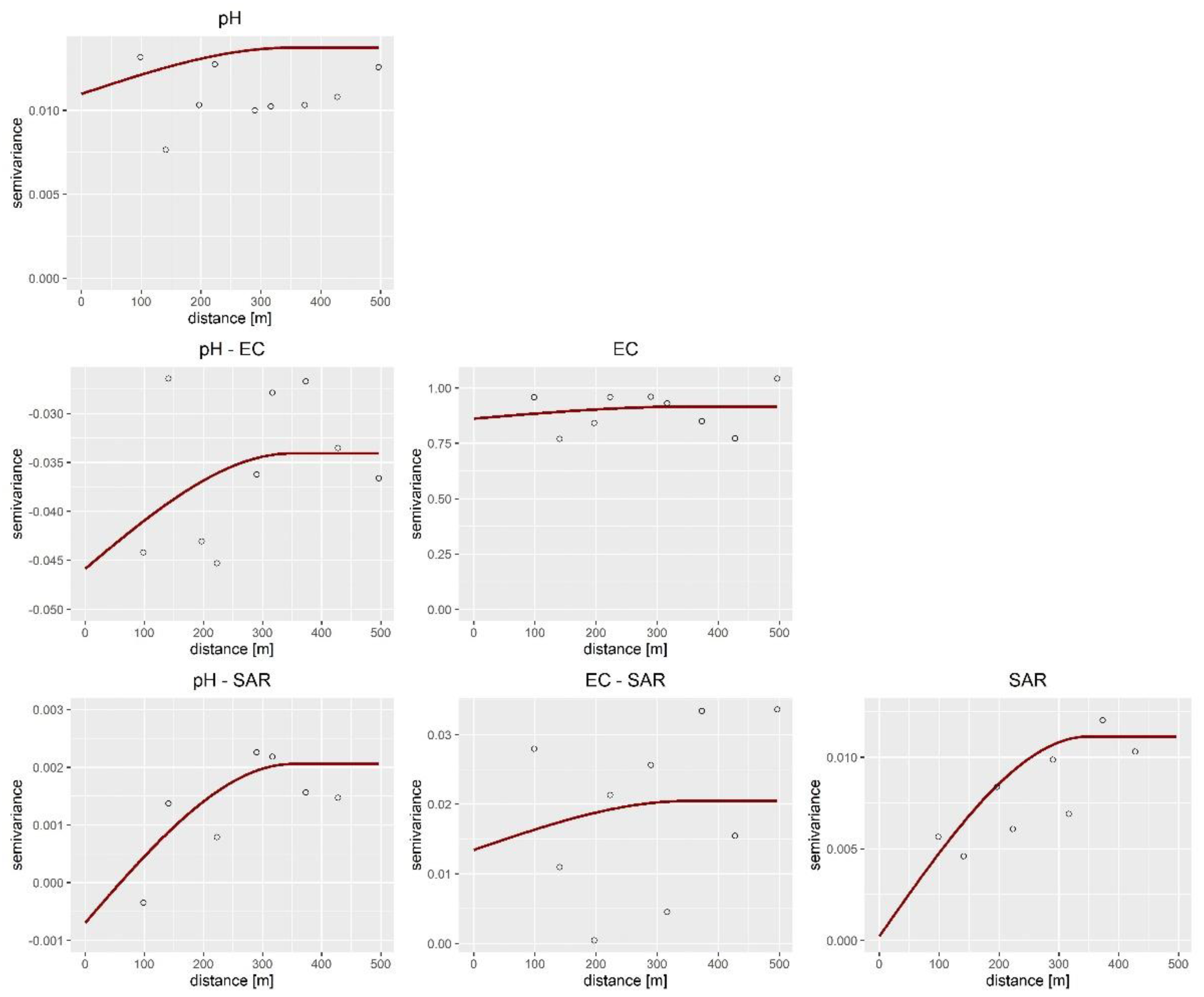
2.4.2. Multivariate Geostatistical Modelling of the Stochastic Residuals
2.5. Validation
3. Results
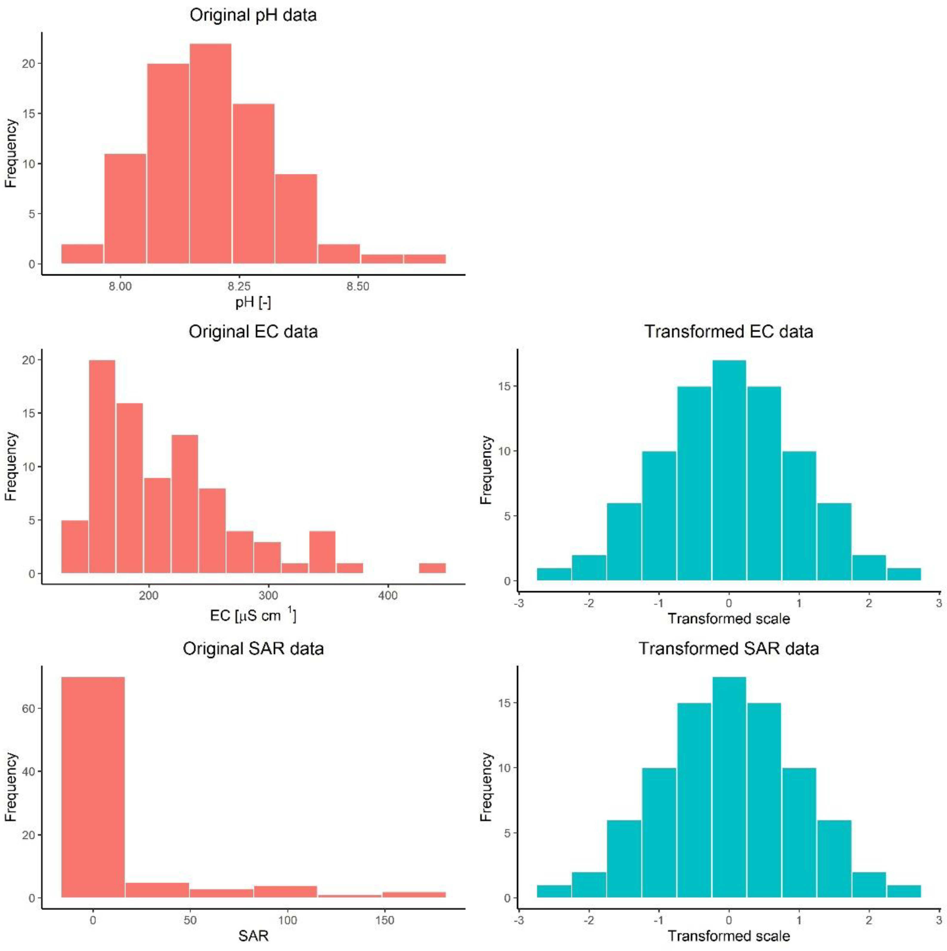
3.1. Soil Survey
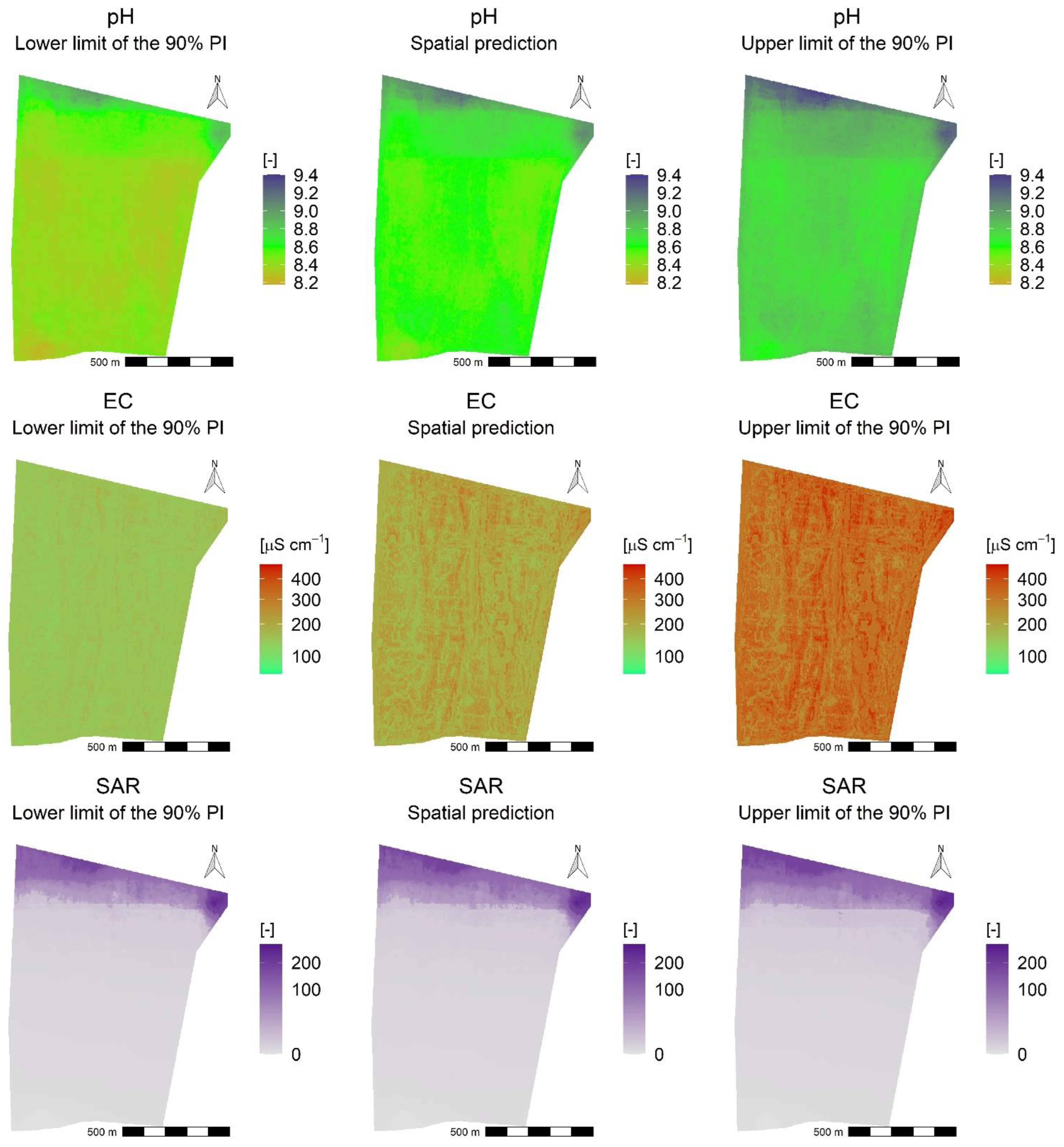
3.2. Spatial Modelling of SAS Indicators
3.3. Performance of Spatial Predictions and Uncertainty Quantifications
4. Discussion
4.1. Ensemble Machine Learning
4.2. Multivariate Geostatistics
4.3. Mapping and Assessment of Salt-Affected Soils
5. Conclusions
- For farmers to indicate:
- -
- The part of the plot where reclamation/drainage works must be carried out and
- -
- Site-specific cultivation can be managed;
- For decision-makers to help them decide:
- -
- the allocation of subsidies.
Author Contributions
Funding
Institutional Review Board Statement
Informed Consent Statement
Data Availability Statement
Acknowledgments
Conflicts of Interest
References
- Stolte, J.; Tesfai, M.; Oygarden, L.; Kvaerno, S.; Keizer, J.; Verheijen, F.; Panagos, P.; Ballabio, C.; Hessel, R. Soil Threats in Europe: Status, Methods, Drivers and Effects on Ecosystem Services. 2016. Available online: https://esdac.jrc.ec.europa.eu/content/soil-threats-europe-status-methods-drivers-and-effects-ecosystem-services (accessed on 1 June 2022).
- Daliakopoulos, I.N.; Tsanis, I.K.; Koutroulis, A.; Kourgialas, N.N.; Varouchakis, A.E.; Karatzas, G.P.; Ritsema, C.J. The Threat of Soil Salinity: A European Scale Review. Sci. Total Environ. 2016, 573, 727–739. [Google Scholar] [CrossRef] [PubMed]
- Majeed, A.; Muhammad, Z. Salinity: A Major Agricultural Problem-Causes, Impacts on Crop Productivity and Management Strategies. Plant Abiotic Stress Toler. Agron. Mol. Biotechnol. Approaches 2019, 83–99. [Google Scholar] [CrossRef]
- Huang, J.; Hartemink, A.E. Soil and Environmental Issues in Sandy Soils. Earth-Sci. Rev. 2020, 208, 103295. [Google Scholar] [CrossRef]
- Singh, A. Soil Salinity: A Global Threat to Sustainable Development. Soil Use Manag. 2022, 38, 39–67. [Google Scholar] [CrossRef]
- Tomaz, A.; Palma, P.; Alvarenga, P.; Gonçalves, M.C. Soil Salinity Risk in a Climate Change Scenario and Its Effect on Crop Yield. Clim. Chang. Soil Interact. 2020, 351–396. [Google Scholar] [CrossRef]
- Ferreira, C.S.S.; Seifollahi-Aghmiuni, S.; Destouni, G.; Ghajarnia, N.; Kalantari, Z. Soil Degradation in the European Mediterranean Region: Processes, Status and Consequences. Sci. Total Environ. 2022, 805, 150106. [Google Scholar] [CrossRef]
- Omuto, C.T.; Vargas, R.R.; El Mobarak, A.M.; Mohamed, N.; Viatkin, K.; Yigini, Y. Mapping of Salt-Affected Soils: Technical Manual; FAO: Rome, Italy, 2020. [Google Scholar]
- Szatmári, G.; Bakacsi, Z.; Laborczi, A.; Petrik, O.; Pataki, R.; Tóth, T.; Pásztor, L. Elaborating Hungarian Segment of the Global Map of Salt-Affected Soils (GSSmap): National Contribution to an International Initiative. Remote Sens. 2020, 12, 4073. [Google Scholar] [CrossRef]
- Jenny, H. Factors of Soil Formation: A System of Quantitative Pedology; McGraw-Hill: New York, NY, USA, 1941. [Google Scholar]
- Tóth, T.; Gallai, B.; Novák, T.; Czigány, S.; Makó, A.; Kocsis, M.; Árvai, M.; Mészáros, J.; László, P.; Koós, S.; et al. Practical Evaluation of Four Classification Levels of Soil Taxonomy, Hungarian Classification and WRB in Terms of Biomass Production in a Salt-Affected Alluvial Plot. Geoderma 2022, 410, 115666. [Google Scholar] [CrossRef]
- Terres, J.; Toth, T.; Wania, A.; Hagyo, A.; Koeble, R.; Nisini Scacchiafichi, L. Updated Guidelines for Applying Common Criteria to Identify Agricultural Areas with Natural Constraints; JRC: Tokyo, Japan, 2016. [Google Scholar]
- Szabolcs, I. Review of Research on Salt Affected Soils. Nat. Resour. Res. 1979. [Google Scholar] [CrossRef]
- Sigmond, E. Hungarian Alkali Soils and Methods of Their Reclamation. In Special Publication Issued by the California Agricultural Experiment Station; University of California Printing Office: Berkeley, CA, USA, 1927. [Google Scholar]
- Szabolcs, I. Salt-Affected Soils; CRC Press: Boca Raton, FL, USA, 1989. [Google Scholar]
- Szabolcs, I. European Solonetz Soils and Their Reclamation; Akadémia Kiadó: Budapest, Hungary, 1971. [Google Scholar]
- Tóth, T.; Szendrei, G. A Hazai Szikes Talajok És a Szikesedés Valamint a Sófelhalmozódási Folyamatok Rövid Jellemzése. Topogr. Mineral. Hungariae 2006, 9, 7–20. [Google Scholar]
- Mádlné Szőnyi, J.; Simon, S.; Tóth, J.; Pogácsás, G. Connection between Surface and Groundwaters in the Case of Kelemen-Lake and Kolon-Lake. Általános Földtani Szle. 2005, 30, 93–110. [Google Scholar]
- Bakacsi, Z.; Kuti, L. Agrogeological Investigation on a Salt Affected Landscape in the Danube Valley, Hungary. Agrokémia és Talajt. 1998, 47, 29–38. [Google Scholar]
- Arany, S. A Hortobágyi Ősi Szíkes Legelőkön Végzett Talajfelvételek. Kísérletügyi Közlemények Pallas részvénytársaság sajtója 1926, 29, 48–71. [Google Scholar]
- Magyar, P. Adatok a Hortobágy Növényszociológiai És Geobotanikai Viszonyaihoz. Erdészeti kisérletek 1928, 30, 26–63. [Google Scholar]
- Szabolcs, I. Hortobágy Talajai; Mezőgazdasági Kiadó: Budapest, Hungary, 1954. [Google Scholar]
- Minasny, B.; McBratney, A.B. Digital Soil Mapping: A Brief History and Some Lessons. Geoderma 2016, 264, 301–311. [Google Scholar] [CrossRef]
- Lagacherie, P.; McBratney, A.B. Spatial Soil Information Systems and Spatial Soil Inference Systems: Perspectives for Digital Soil Mapping. Dev. Soil Sci. 2007, 31, 3–22. [Google Scholar]
- Szatmári, G.; Pásztor, L.; Heuvelink, G.B.M. Estimating Soil Organic Carbon Stock Change at Multiple Scales Using Machine Learning and Multivariate Geostatistics. Geoderma 2021, 403, 115356. [Google Scholar] [CrossRef]
- Heuvelink, G.B.M.; Angelini, M.E.; Poggio, L.; Bai, Z.; Batjes, N.H.; van den Bosch, R.; Bossio, D.; Estella, S.; Lehmann, J.; Olmedo, G.F.; et al. Machine Learning in Space and Time for Modelling Soil Organic Carbon Change. Eur. J. Soil Sci. 2020. [Google Scholar] [CrossRef]
- Styc, Q.; Lagacherie, P. Uncertainty Assessment of Soil Available Water Capacity Using Error Propagation: A Test in Languedoc-Roussillon. Geoderma 2021, 391, 114968. [Google Scholar] [CrossRef]
- Helfenstein, A.; Mulder, V.L.; Heuvelink, G.B.M.; Okx, J.P. Tier 4 Maps of Soil PH at 25 m Resolution for the Netherlands. Geoderma 2022, 410, 115659. [Google Scholar] [CrossRef]
- Chen, S.; Mulder, V.L.; Martin, M.P.; Walter, C.; Lacoste, M.; Richer-de-Forges, A.C.; Saby, N.P.A.; Loiseau, T.; Hu, B.; Arrouays, D. Probability Mapping of Soil Thickness by Random Survival Forest at a National Scale. Geoderma 2019, 344, 184–194. [Google Scholar] [CrossRef]
- Keskin, H.; Grunwald, S. Regression Kriging as a Workhorse in the Digital Soil Mapper’s Toolbox. Geoderma 2018, 326, 22–41. [Google Scholar] [CrossRef]
- Sahbeni, G.; Székely, B. Spatial Modeling of Soil Salinity Using Kriging Interpolation Techniques: A Study Case in the Great Hungarian Plain. Eurasian J. Soil Sci. 2022, 11, 102–112. [Google Scholar] [CrossRef]
- Brus, D.J.; Kempen, B.; Heuvelink, G.B.M. Sampling for Validation of Digital Soil Maps. Eur. J. Soil Sci. 2011, 62, 394–407. [Google Scholar] [CrossRef]
- Heuvelink, G.B.M. Uncertainty and Uncertainty Propagation in Soil Mapping and Modelling. In Pedometrics; Springer: Cham, Germany, 2018; pp. 439–461. [Google Scholar]
- Szatmári, G.; Pásztor, L. Comparison of Various Uncertainty Modelling Approaches Based on Geostatistics and Machine Learning Algorithms. Geoderma 2019, 337, 1329–1340. [Google Scholar] [CrossRef]
- Mishra, U.; Gautam, S.; Riley, W.J.; Hoffman, F.M. Ensemble Machine Learning Approach Improves Predicted Spatial Variation of Surface Soil Organic Carbon Stocks in Data-Limited Northern Circumpolar Region. Front. Big Data 2020, 3, 528441. [Google Scholar] [CrossRef]
- Brungard, C.; Nauman, T.; Duniway, M.; Veblen, K.; Nehring, K.; White, D.; Salley, S.; Anchang, J. Regional Ensemble Modeling Reduces Uncertainty for Digital Soil Mapping. Geoderma 2021, 397, 114998. [Google Scholar] [CrossRef]
- Kadavi, P.R.; Lee, C.W.; Lee, S. Application of Ensemble-Based Machine Learning Models to Landslide Susceptibility Mapping. Remote Sens. 2018, 10, 1252. [Google Scholar] [CrossRef]
- Hengl, T.; Miller, M.A.E.; Križan, J.; Shepherd, K.D.; Sila, A.; Kilibarda, M.; Antonijević, O.; Glušica, L.; Dobermann, A.; Haefele, S.M.; et al. African Soil Properties and Nutrients Mapped at 30 m Spatial Resolution Using Two-Scale Ensemble Machine Learning. Sci. Reports 2021, 11, 1–18. [Google Scholar] [CrossRef]
- Zhang, C.; Ma, Y. Ensemble Machine Learning; Springer: New York, NY, USA, 2012. [Google Scholar]
- Seni, G.; Elder, J.F. Ensemble Methods in Data Mining. Springer International Publishing, 2010; Available online: https://link.springer.com/content/pdf/bfm%3A978-3-031-01899-2%2F1 (accessed on 1 June 2022).
- Polikar, R. Ensemble Learning. Ensemble Mach. Learn. 2012, 1–34. [Google Scholar] [CrossRef]
- El Badawi, H.; Azais, F.; Bernard, S.; Comte, M.; Kerzerho, V.; Lefevre, F. Use of Ensemble Methods for Indirect Test of RF Circuits: Can It Bring Benefits? In Proceedings of the 2019 IEEE Latin American Test Symposium (LATS), Santiago, Chile, 11–13 March 2019. [CrossRef]
- Mulder, V.L.; de Bruin, S.; Schaepman, M.E.; Mayr, T.R. The Use of Remote Sensing in Soil and Terrain Mapping—A Review. Geoderma 2011, 162, 1–19. [Google Scholar] [CrossRef]
- Dwivedi, R.S. Remote Sensing of Soils; Springer: Berlin/Heidelberg, Germany, 2017; ISBN 9783662537404. [Google Scholar]
- Pásztor, L.; Takács, K. Remote Sensing in Soil Mapping—A Review. Agrokémia és Talajt. 2014, 63, 353–370. [Google Scholar] [CrossRef]
- Wang, N.; Peng, J.; Chen, S.; Huang, J.; Li, H.; Biswas, A.; He, Y.; Shi, Z. Improving Remote Sensing of Salinity on Topsoil with Crop Residues Using Novel Indices of Optical and Microwave Bands. Geoderma 2022, 422, 115935. [Google Scholar] [CrossRef]
- Sahbeni, G. A PLSR Model to Predict Soil Salinity Using Sentinel-2 MSI Data. Open Geosci. 2021, 13, 977–987. [Google Scholar] [CrossRef]
- Dövényi, Z. Inventory of Microregions in Hungary, 2nd ed.; Hungarian Academy of Sciences, Geographical Research Institute: Budapest, Hungary, 2010. [Google Scholar]
- IUSS Working Group. WRB World Reference Base for Soil Resources 2014, Update 2015 International Soil Classification System for Naming Soils and Creating Legends for Soil Maps; World Soil Resources Reports No. 106; IUSS Working Group: Rome, Itlay, 2015. [Google Scholar]
- Richards, L.A. Diagnosis and Improvement of Saline Alkali Soils; US Department of Agriculture: Washington, DC, USA, 1954. [Google Scholar]
- Conrad, O.; Bechtel, B.; Bock, M.; Dietrich, H.; Fischer, E.; Gerlitz, L.; Wehberg, J.; Wichmann, V.; Böhner, J. System for Automated Geoscientific Analyses (SAGA) v. 2.1.4. Geosci. Model Dev. 2015, 8, 1991–2007. [Google Scholar] [CrossRef]
- Shrestha, R.P. Relating Soil Electrical Conductivity to Remote Sensing and Other Soil Properties for Assessing Soil Salinity in Northeast Thailand. Land Degrad. Dev. 2006, 17, 677–689. [Google Scholar] [CrossRef]
- Nield, S.J.; Boettinger, J.L.; Ramsey, R.D. Digitally Mapping Gypsic and Natric Soil Areas Using Landsat ETM Data. Soil Sci. Soc. Am. J. 2007, 71, 245–252. [Google Scholar] [CrossRef]
- Dehni, A.; Lounis, M. Remote Sensing Techniques for Salt Affected Soil Mapping: Application to the Oran Region of Algeria. Procedia Eng. 2012, 33, 188–198. [Google Scholar] [CrossRef]
- Stein, A.; Corsten, L.C.A. Universal Kriging and Cokriging as a Regression Procedure. Biometrics 1991, 47, 575–587. [Google Scholar] [CrossRef]
- Myers, D.E. Matrix Formulation of Co-Kriging. J. Int. Assoc. Math. Geol. 1982, 14, 249–257. [Google Scholar] [CrossRef]
- McBratney, A.B.; Mendonça Santos, M.L.; Minasny, B. On Digital Soil Mapping. Geoderma 2003, 117, 3–52. [Google Scholar] [CrossRef]
- Wackernagel, H. Multivariate Geostatistics; Springer: Berlin/Heidelberg, Germany, 2003. [Google Scholar]
- Goovaerts, P. Geostatistics for Natural Resources Evaluation; Oxford University Press: New York, NY, USA; Oxford, UK, 1997; ISBN 9780195115383. [Google Scholar]
- Cressie, N.A.C. Statistics for Spatial Data; Wiley: Hoboken, NJ, USA, 1993. [Google Scholar]
- Geiger, J. Some Thoughts on the Pre- and Post-Processing in Sequential Gaussian Simulation and Their Effects on Reservoir Characterization. In New Horizons in Central European Geomathematics, Geostatistics and Geoinformatics; Geiger, J., Pál-Molnár, E., Malvic, T., Eds.; GeoLitera: Szeged, Hungary, 2012; pp. 17–34. [Google Scholar]
- Deutsch, C.V.; Journel, A.G. GSLIB: Geostatistical Software Library and User’s Guide; Oxford University Press: New York, UK, 1998; ISBN 9780195100150. [Google Scholar]
- Breiman, L. Random Forests. Mach. Learn. 2001, 45, 5–32. [Google Scholar] [CrossRef]
- Wright, M.N.; Ziegler, A. Ranger: A Fast Implementation of Random Forests for High Dimensional Data in C++ and R. J. Stat. Softw. 2017, 77, 1–17. [Google Scholar] [CrossRef]
- Chen, T.; Guestrin, C. XGBoost: A Scalable Tree Boosting System. In Proceedings of the 22nd ACM SIGKDD International Conference on Knowledge Discovery and Data Mining, San Francisco, CA, USA, 13–17 August 2016; pp. 785–794. [Google Scholar] [CrossRef]
- Pisner, D.A.; Schnyer, D.M. Support Vector Machine. Mach. Learn. Methods Appl. Brain Disord. 2020, 101–121. [Google Scholar] [CrossRef]
- Vapnik, V.; Golowich, S.; Smolal, A. Support Vector Method for Function Approximation, Regression Estimation and Signal Processing. Adv. Neural Inf. Processing Syst. 1996, 9. [Google Scholar] [CrossRef]
- Zhu, A.X. Mapping Soil Landscape as Spatial Continua: The Neural Network Approach. Water Resour. Res. 2000, 36, 663–677. [Google Scholar] [CrossRef]
- Friedman, J.; Hastie, T.; Tibshirani, R. Regularization Paths for Generalized Linear Models via Coordinate Descent. J. Stat. Softw. 2010, 33, 1. [Google Scholar] [CrossRef]
- Hengl, T. Landmap. 2021. [Google Scholar]
- R Core Team. A Language and Environment for Statistical Computing; The R Foundation—The R Project for Statistical Computing: Vienna, Austria, 2013. Available online: http://www.R-project.org/ (accessed on 1 June 2022).
- Bischl, B.; Lang, M.; Kotthoff, L.; Schiffner, J.; Richter, J.; Studerus, E.; Casalicchio, G.; Jones, Z.M. Mlr: Machine Learning in R. J. Mach. Learn. Res. 2016, 17, 5938–5942. [Google Scholar]
- Hengl, T.; Parente, L.; Bonannella, C. Spatial and Spatiotemporal Interpolation/Prediction Using Ensemble Machine Learning. 2022. Available online: https://opengeohub.github.io/spatial-prediction-eml/ (accessed on 1 June 2022). [CrossRef]
- Heuvelink, G. Uncertainty Quantification of GlobalSoilMap Products. In GlobalSoilMap; CRC Press: Boca Raton, FL, USA, 2014; pp. 335–340. [Google Scholar]
- Lin, L.I.-K. A Concordance Correlation Coefficient to Evaluate Reproducibility. Biometrics 1989, 45, 255–268. [Google Scholar] [CrossRef]
- Nash, J.E.; Sutcliffe, J.V. River Flow Forecasting through Conceptual Models Part I—A Discussion of Principles. J. Hydrol. 1970, 10, 282–290. [Google Scholar] [CrossRef]
- Paz, A.M.; Castanheira, N.; Farzamian, M.; Paz, M.C.; Gonçalves, M.C.; Monteiro Santos, F.A.; Triantafilis, J. Prediction of Soil Salinity and Sodicity Using Electromagnetic Conductivity Imaging. Geoderma 2020, 361, 114086. [Google Scholar] [CrossRef]
- Li, H.Y.; Shi, Z.; Webster, R.; Triantafilis, J. Mapping the Three-Dimensional Variation of Soil Salinity in a Rice-Paddy Soil. Geoderma 2013, 195, 31–41. [Google Scholar] [CrossRef]
- Lück, E.; Gebbers, R.; Ruehlmann, J.; Spangenberg, U. Electrical Conductivity Mapping for Precision Farming. Near Surf. Geophys. 2009, 7, 15–26. [Google Scholar] [CrossRef]
- Hateffard, F.; Dolati, P.; Heidari, A.; Zolfaghari, A.A. Assessing the Performance of Decision Tree and Neural Network Models in Mapping Soil Properties. J. Mt. Sci. 2019, 16, 1833–1847. [Google Scholar] [CrossRef]
- John, K.; Isong, I.A.; Kebonye, N.M.; Ayito, E.O.; Agyeman, P.C.; Afu, S.M. Using Machine Learning Algorithms to Estimate Soil Organic Carbon Variability with Environmental Variables and Soil Nutrient Indicators in an Alluvial Soil. Land 2020, 9, 487. [Google Scholar] [CrossRef]
- Odeh, I.O.A.; McBratney, A.B.; Chittleborough, D.J. Further Results on Prediction of Soil Properties from Terrain Attributes: Heterotopic Cokriging and Regression-Kriging. Geoderma 1995, 67, 215–226. [Google Scholar] [CrossRef]
- Lark, R.M.; Ander, E.L.; Cave, M.R.; Knights, K.V.; Glennon, M.M.; Scanlon, R.P. Mapping Trace Element Deficiency by Cokriging from Regional Geochemical Soil Data: A Case Study on Cobalt for Grazing Sheep in Ireland. Geoderma 2014, 226–227, 64–78. [Google Scholar] [CrossRef]
- Wackernagel, H. Cokriging versus Kriging in Regionalized Multivariate Data Analysis. Geoderma 1994, 62, 83–92. [Google Scholar] [CrossRef]
- Vaysse, K.; Lagacherie, P. Evaluating Digital Soil Mapping Approaches for Mapping GlobalSoilMap Soil Properties from Legacy Data in Languedoc-Roussillon (France). Geoderma Reg. 2015, 4, 20–30. [Google Scholar] [CrossRef]
- Szatmári, G.; Barta, K.; Pásztor, L. An Application of a Spatial Simulated Annealing Sampling Optimization Algorithm to Support Digital Soil Mapping. Hungarian Geogr. Bull. 2015, 64, 35–48. [Google Scholar] [CrossRef]
- Brus, D.J. Sampling for Digital Soil Mapping: A Tutorial Supported by R Scripts. Geoderma 2019, 338, 464–480. [Google Scholar] [CrossRef]
- Burgess, T.M.; Webster, R.; McBratney, A.B. Optimal Interpolation and Isarithmic Mapping of Soil Properties. IV Sampling Strategy. J. Soil Sci. 1981, 32, 643–659. [Google Scholar] [CrossRef]
- de Gruijter, J.J.; Bierkens, M.F.P.; Brus, D.J.; Knotters, M. Sampling for Natural Resource Monitoring; Springer: Berlin/Heidelberg, Germany, 2006; ISBN 978-3-540-22486-0. [Google Scholar]
- Marchant, B.P.; Lark, R.M. Optimized Sample Schemes for Geostatistical Surveys. Math. Geol. 2007, 39, 113–134. [Google Scholar] [CrossRef]
- Lark, R.M.; Marchant, B.P. How Should a Spatial-Coverage Sample Design for a Geostatistical Soil Survey Be Supplemented to Support Estimation of Spatial Covariance Parameters? Geoderma 2018, 319, 89–99. [Google Scholar] [CrossRef]
- Wadoux, A.M.J.C.; Marchant, B.P.; Lark, R.M. Efficient Sampling for Geostatistical Surveys. Eur. J. Soil Sci. 2019, 70, 975–989. [Google Scholar] [CrossRef]
- Tóth, T.; Várallyay, G. Past, Present and Future of the Hungarian Classification of Salt-Affected Soils. Soil Classif. 2001, 125–135. [Google Scholar]
- Van Orshoven, J.; Terres, J.-M.; Tóth, T. Updated Common Bio-Physical Criteria to Define Natural Constraints for Agriculture in Europe; Office for Official Publications of the European Communities: Luxembourg, 2012. [Google Scholar]
- Pásztor, L.; Szabó, J.; Bakacsi, Z.; László, P.; Dombos, M. Large-Scale Soil Maps Improved by Digital Soil Mapping and GIS-Based Soil Status Assessment. Agrokémia és Talajt. 2007, 55, 79–88. [Google Scholar] [CrossRef]
- Nabiollahi, K.; Taghizadeh-Mehrjardi, R.; Shahabi, A.; Heung, B.; Amirian-Chakan, A.; Davari, M.; Scholten, T. Assessing Agricultural Salt-Affected Land Using Digital Soil Mapping and Hybridized Random Forests. Geoderma 2021, 385, 114858. [Google Scholar] [CrossRef]
- Kvoda, V.A.; van den Berg, C.; Hagan, R.M. Irrigation, Drainage and Salinity; Hutchinson/FAO/UNESCO, 1973. Available online: https://unesdoc.unesco.org/ark:/48223/pf0000005702 (accessed on 1 June 2022).
- Buzási, A.; Pálvölgyi, T.; Esses, D. Drought-Related Vulnerability and Its Policy Implications in Hungary. Mitig. Adapt. Strateg. Glob. Chang. 2021, 26, 1–20. [Google Scholar] [CrossRef]
- Sparks, D.L. Environmental Soil Chemistry; Academic Press: Cambridge, MA, USA, 1995; ISBN 9780126564457. [Google Scholar]


| Factors of Soil Formation [10] | Environmental Covariates | Source |
|---|---|---|
| Soil surface | Brightness index | Sentinel-2 |
| Normalized difference salinity index | ||
| Salinity index 1-5 | ||
| Salinity ratio | ||
| Visible infrared salinity index | ||
| Green band | ||
| Red band | ||
| Near-infrared band | ||
| Short-wave infrared-1 | ||
| Short-wave infrared-2 | ||
| Topography | Elevation | DEM |
| Slope | ||
| Aspect | ||
| Topographic position index | ||
| Terrain ruggedness index | ||
| Roughness | ||
| Flow direction | ||
| Catchment area | ||
| Modified catchment area | ||
| Diurnal anisotropic heating | ||
| LS factor (slope length factor) | ||
| Mass balance index | ||
| MRRTF | ||
| MRVBF | ||
| Topographic wetness index | ||
| Organisms | Normalized difference vegetation index | Sentinel-2 |
| Soil adjusted vegetation index | ||
| Vegetation soil salinity index |
| SAS Indicators | Unit | Min | Max | Mean | SD |
|---|---|---|---|---|---|
| EC | µS cm−1 | 136.4 | 428.0 | 214.0 | 59.94 |
| pH | - | 7.90 | 8.79 | 8.201 | 0.15 |
| SAR | - | 0.13 | 181.0 | 15.79 | 37.32 |
| ML Algorithms | R2 | RMSE | MAE | ||||||
|---|---|---|---|---|---|---|---|---|---|
| pH | EC | SAR | pH | EC | SAR | pH | EC | SAR | |
| RF | 0.36 | 0.39 | 0.96 | 0.12 | 0.97 | 0.21 | 0.10 | 0.79 | 0.09 |
| XGBoost | 0.09 | - | 0.91 | 5.42 | - | 0.83 | 5.42 | - | 0.65 |
| NN | 0.09 | - | 0.10 | 0.15 | - | 1.00 | 0.11 | - | 0.81 |
| SVM | 0.22 | - | 0.90 | 0.13 | - | 0.33 | 0.10 | - | 0.21 |
| GLM | 0.12 | - | 0.95 | 0.14 | - | 0.27 | 0.11 | - | 0.14 |
| SuperLearner | 0.43 | - | 0.96 | 0.11 | - | 0.20 | 0.09 | - | 0.11 |
| SAS Indicators | ME | RMSE | CCC | NSE |
|---|---|---|---|---|
| pH | 0.001 | 0.11 | 0.59 | 0.41 |
| EC | 0.001 | 0.86 | 0.39 | 0.24 |
| SAR | 0.007 | 0.22 | 0.97 | 0.95 |
Publisher’s Note: MDPI stays neutral with regard to jurisdictional claims in published maps and institutional affiliations. |
© 2022 by the authors. Licensee MDPI, Basel, Switzerland. This article is an open access article distributed under the terms and conditions of the Creative Commons Attribution (CC BY) license (https://creativecommons.org/licenses/by/4.0/).
Share and Cite
Hateffard, F.; Balog, K.; Tóth, T.; Mészáros, J.; Árvai, M.; Kovács, Z.A.; Szűcs-Vásárhelyi, N.; Koós, S.; László, P.; Novák, T.J.; et al. High-Resolution Mapping and Assessment of Salt-Affectedness on Arable Lands by the Combination of Ensemble Learning and Multivariate Geostatistics. Agronomy 2022, 12, 1858. https://doi.org/10.3390/agronomy12081858
Hateffard F, Balog K, Tóth T, Mészáros J, Árvai M, Kovács ZA, Szűcs-Vásárhelyi N, Koós S, László P, Novák TJ, et al. High-Resolution Mapping and Assessment of Salt-Affectedness on Arable Lands by the Combination of Ensemble Learning and Multivariate Geostatistics. Agronomy. 2022; 12(8):1858. https://doi.org/10.3390/agronomy12081858
Chicago/Turabian StyleHateffard, Fatemeh, Kitti Balog, Tibor Tóth, János Mészáros, Mátyás Árvai, Zsófia Adrienn Kovács, Nóra Szűcs-Vásárhelyi, Sándor Koós, Péter László, Tibor József Novák, and et al. 2022. "High-Resolution Mapping and Assessment of Salt-Affectedness on Arable Lands by the Combination of Ensemble Learning and Multivariate Geostatistics" Agronomy 12, no. 8: 1858. https://doi.org/10.3390/agronomy12081858