1. Introduction
Precise and automatic monitoring of the satisfaction of safety constraints imposed on cyber-physical systems is of utmost importance in a variety of settings: traditionally, it facilitates offline or, if supported by the monitoring algorithm, online system debugging as well as, if pursued online in real-time, the demand-driven activation of safety and fallback mechanisms in safety-oriented architectures as soon as a safety-critical system leaves its operational domain or exposes unexpected behavior. An application domain of growing importance is the safety assurance of autonomous systems, such as unmanned aircraft. Such systems are increasingly equipped with decision-making components that carry out complex missions in areas such as transport, mapping and surveillance, and agriculture. In such applications the monitor plays a critical role in assessing system health conditions (such as sensor cross-validation) and regulatory constraints like geo-fencing, which prevents the aircraft from entering protected airspace [
1]. More recently, continuous diagnosis in continuous agile development processes like DevOps has caught interest and provides a further field of application [
2]. Of special interest here is the provisioning of flexible languages for the specification of monitors, as the pertinent safety constraints vary tremendously across systems and application domains. Answering this quest, Signal Temporal Logic (STL) [
3] and similar linear-time temporal logics have been designed for classifying the time-dependent signals originating from continuous-state or hybrid-state dynamical systems according to formal specifications, alongside efficient stream processing languages targeted towards online monitoring [
1]. These highly expressive specification languages do, however, induce the follow-up quest for efficient automatic implementation of monitoring algorithms by means of translation from the formal safety or monitoring specifications.
There consequently is a rich body of work on synthesis of monitors from logical specifications of temporal or spatio-temporal type (cf. [
4] for an overview), with nowadays even robust industrial tools being available [
5], as well as hard real-time capable stream-based execution mechanisms for on-line monitoring of even more expressive monitoring languages [
1]. Most of the suggested algorithms do, however, not address the problem of epistemic uncertainty due to environmental sensing, with the monitoring algorithms rather taking sensor values and timestamps as is and ignoring their inherent imprecision. Such imprecisions are unavoidable in applications such as autonomous aircraft due to wind and other external influences. A notable exception is provided by robust quantitative interpretations of temporal logic, which can cope with inaccuracy in timestamps [
6] as well as in sensor values [
7]. The corresponding robust monitoring approaches [
8] support a metric, yet not stochastic, error model, and consequently ignore the fact that repeated measurements provide additional evidence, thus ignoring the wisdom and toolset from metrology concerning state estimation [
9,
10], consequently providing extremely pessimistic verdicts [
11]. Overcoming the latter problem would require equipping the pertinent logics, like Signal Temporal Logic [
7], with a truly stochastic (i.e., reporting a likelihood of satisfaction over a stochastic model) rather than a trace-based metric semantics (reporting slackness of the signal values observed across a single trace towards change of truth value of the formula). This remains the subject of our further research.
In this article, we do nevertheless show that already in a metric setting of interval-bounded measurement error, as employed in [
12], refined algorithms addressing the relation between successive measurements are possible. Visconti et al. [
12] have previously addressed the issue of inexact measurements metrically, taking up the simple model of interval-bounded independent per-sample error which is unrelated across samples in the sense of chosen afresh upon every sample. We expand their analysis by decomposing the error into an unknown yet fixed offset and an independent per-sample error and show that in this setting, monitoring of temporal properties no longer coincides with collecting Boolean combinations of predicates evaluated pointwise over best-possible per-sample state estimates, but can be genuinely more informative in that it infers determinate truth values for monitoring conditions that interval-based evaluation remains inconclusive about. For the model-free as well as for the (certain or uncertain) linear model-based case, we provide optimal evaluation algorithms based on affine arithmetic [
13] and SAT modulo theory solving over linear arithmetic [
14,
15]. Beyond uncertain sensing, we also address the issues of partial observation (w.r.t. both state variables and time instants) in uncertain linear systems. In all these cases, the reductions to proof obligations in affine arithmetic provide conclusive monitoring verdicts in many cases where interval-valued state estimations and subsequent interval-based evaluation of temporal monitoring properties inherently remains inconclusive, which we demonstrate by means of examples. We furthermore prove that our affine-arithmetic reductions are optimal in that they are as precise as a monitor operating under metric uncertainty can possibly be: they do not only provide sound verdicts throughout, but are also optimally informed in that they always yield a conclusive verdict whenever this is justified by the formula semantics. Any reduction to even richer extensions of interval arithmetic, like [
16], would consequently fail to provide additional gains in precision.
To achieve these results, we first in
Section 2 review the definition of Signal Temporal Logic [
7], which we use as the formalism of choice for illustration. We then provide the metric error model for measurements (
Section 3) and based on it define the monitoring problem under metric uncertainty (
Section 4) including rigorous criteria for soundness, completeness, and precision of monitoring algorithms. The subsequent two sections develop optimal monitoring algorithms based on reductions to affine arithmetic, where
Section 5 covers the model-free case and
Section 6 treats optimal monitoring when a (potentially uncertain) affine model of system dynamics is given. Both sections provide illustrative examples of the constructions.
Section 7, finally, investigates the worst-case complexity of the monitoring problem under uncertainty.
2. Signal Temporal Logic
Signal temporal logic (STL) [
3] is a linear-time temporal logic designed as a formal specification language for classifying the time-dependent signals originating from continuous-state or hybrid-state dynamical systems. Its development has been motivated by a need for a flexible yet rigorous language systematising the monitoring of cyber-physical systems. Especially relevant to such monitoring applications is the bounded-time fragment of STL defined as follows.
Definition 1. Formulae ϕ of bounded-time STL
are defined by the Backus-Naur formwhere is a predefined set of signal names. We demand that in . The constant ⊥, further Boolean connectives like ∧ or ⇒, and further modalities or can be defined as usual: for example, is an abbreviation for and is an abbreviation for given the discrete nature of the time model.
Note that the above definition confines state expressions
g to be linear combinations of signals, in contrast to the standard definition [
3] of STL, which permits more general state expressions. The reason for adopting this restriction is that it permits exact results in monitoring, whereas more general state expressions can well be treated in our framework by exploiting standard affine-arithmetic approximations [
13], yet completeness would be lost due to overapproximations induced by a strife for soundness.
For the same reasons, we adopt a discrete-time semantics, as issues of continuous interpolation between time instants of measurements have been addressed before in [
17]. Adopting those mechanisms, continuous-time dynamic systems and continuous-time interpretation of STL can be treated as well, yet would again resort to affine approximations at the price of sacrificing exactness of the monitoring algorithm.
The semantics of STL builds on the notion of a trajectory:
Definition 2. A state valuation σ is a mapping of signal names to real values, i.e., a function . The set of all state valuations is denoted by Σ. A(discrete time) trajectory is a mapping from time instants, where time is identified with the natural numbers , to state valuations.
Satisfaction
of an STL formula ϕ by a (discrete-time) trajectory τ at time instant , denoted as , is defined recursively as Note that the truth value of an STL formula
over a trajectory
at time
t thus can be decided at time
if the values
are known for all time instants
and all variable names
x occurring in
, where
is defined as follows:
Unfortunately, the ground-truth values of are frequently not directly accessible and have to be retrieved via environmental sensing, which is bound to be inexact due to measurement error and partial due to economic and physical constraints on sensor deployment and capabilities. Inaccessibility of the ground truth renders direct decision of STL properties based on the above semantics elusive; we rather need to infer, as far as this is possible, the truth value of an STL monitoring condition from the vague evidence provided by mostly partial and inexact sensing.
3. Imperfect Information Due to Noisy Sensing
The simplest metric model of measurement error is obtained by assuming the error to be interval-bounded and independent across sensors as well as across time instants of measurements, thus pretending that the error incurred when measuring the same physical quantity by the same sensor at different times is uncorrelated. Sensor-based monitoring under such a model of measurement uncertainty can be realized by an appropriate interval lifting of the STL semantics [
12], as standard interval arithmetic (IA) [
18] underlying this lifting reflects an analogous independence assumption.
This independence assumption, however, is infamously known as the dependency (or alias) problem of interval arithmetic in cases where the independence assumption does not actually apply and IA consequently yields an overly conservative approximation instead [
18]. Such overapproximation will obviously also arise when the interval-based monitoring algorithm [
12] is applied in cases where the per-sample error of multiple measurements is not fully independent; the overapproximation then shows by reporting inconclusive monitoring verdicts (due to the interval embedding encoded as the inconclusive truth value interval
) rather than a conclusive truth value
Dependencies between per-sample measurement errors are, however, the rule and not the exception. As a typical example take the usual decomposition of measurement error into a confounding unknown yet fixed sensor offset that remains constant across successive measurements taken by the same sensor, and a random measurement error that varies uncorrelated between samples at different time instants. The upper bounds of these two values refer directly to the two terms “trueness” and “precision” used by the pertinent ISO norm 5725 to describe the accuracy of a measurement method. They are consequently found routinely in data sheets of sensor devices, which we consider to be the contracts between component (i.e., sensor) manufacturer and component user (i.e., the monitor designer) in the sense of contract-based design [
19], implying that all subsequent logical inferences we pursue are relative to satisfaction of the contract by the actual sensor. Within the ISO parlance, precision identifies the grouping or closeness of multiple readings, i.e., the portion of the total error that varies in an unpredictable way between tests or measurements. In contrast, trueness indicates the closeness of the average test results to a reference or true value in the sense of the deviation or offset of the arithmetic mean of a large number of repeated measurements and the true or accepted reference value.
Definition 3. Let S be a sensor observing a signal at times with a maximal sensor offset
of and a maximal random measurement error
of . Let τ be a (ground-truth) trajectory. Then is a possibleS time series over
iff If is an S time series over τ, then we symmetrically say that the trajectory is consistent with and denote this fact by . This notion immediately extends to simultaneous consistency with a set of time series , , to : we denote the fact that trajectory τ satisfies for each by .
Note that the above definition features two additive offsets affecting measurements, the first of which (namely the sensor offset) is uniformly chosen for the whole time series while the second one (the random noise) is chosen independently upon every sample. These errors are absolute in that their magnitude does not depend on the magnitude of the ground truth value, which is a standard model of measurement errors appropriate for many simple sensor designs. In specific settings, e.g., when the dynamic range of a sensor is extended by variable-gain pre-amplification as usual in seismology [
20] or by regulating light flow to optical sensors via an automatically controlled optical aperture, relative error or similar error models may be more appropriate. These can be formulated analogously. For the combination of an absolute offset and a relative per-sample error, e.g., the characteristic Equation (
1) would have to be replaced by
4. The Monitoring Problem
Assume that we want to continuously monitor truth of a safety requirement stated as a bounded-time STL formula. In reality, we can only do so based on a set to of time series of measurements obtained through different sensors to . Each of these sensors is inexact, none can predict the future, and even together they provide only partial introspection into the set of signals generated by the system under monitoring. The problem at hand is to, at any time , generate as precise as possible verdicts about the truth of the monitoring condition at time given the imprecise measurements provided by the sensor array to up to time t.
Doing so requires identifying the full set of ground-truth signals possible given a set of inexact measurements. This, however, coincides with the notion of consistency stated in Definition 3.
Definition 4. Let to be a set of sensors, each qualified by an individual maximum sensor offset and an individual maximum random error , which observe (not necessarily different) signals at (potentially diverse) time instants . Let be the current time and be the time series representing measurements obtained by the different sensors up to time t.
The possible ground truth
associated to the time series to is the set of all trajectories τ satisfying , i.e., being consistent with all available measurements simultaneously. We signify the set of all possible ground truth trajectories corresponding to a set of measurements by The monitoring problem now is to characterize the possible ground truth exactly and to determine the possible truth values of the monitoring condition across the possible ground truth:
Definition 5. Let ϕ be a bounded-time STL formula according to the syntax from Definition 1, be the current time, and , for to , be time series representing measurements obtained by the different sensors up to time t.
Let M be an algorithm taking as arguments a current time t, a vector of time series and computing a verdict in . In the sequel, we denote termination of M with verdict x by .
We say that M is sound iff
- (a)
implies that and
- (b)
implies that
holds for all t and .
M is complete iff M terminates on all t and .
M is conclusive iff
- (c)
implies that
holds for all t and .
We call M exact iff M is sound, conclusive, and complete.
A sound monitor thus provides correct verdicts only, but may refuse decisive verdicts by non-termination or by reporting . A complete monitor always provides some verdict, including . A sound and complete monitor may thus still be uninformative by delivering sound but vacuous verdicts. A conclusive monitor, in contrast, reports only when the evidence provided by the uncertain sensors factually is too weak to determine an actual truth value. An exact monitor, consequently, always provides an as precise verdict as possible.
When striving for such an exact monitoring algorithm, the problem is that the set of ground-truth trajectories corresponding to a given time series of measurements is uncountable in general, namely as soon as or , i.e., whenever measurements are imprecise. An enumeration of , and thereby a straightforward lifting of the standard monitoring algorithms is impossible. Any algorithmic approach to STL monitoring under imprecise observation consequently has to resort to a non-trivial finite computational representation of , which is the issue of the next two sections.
5. Exact Monitoring under Imperfect Information: The Model-Free Case
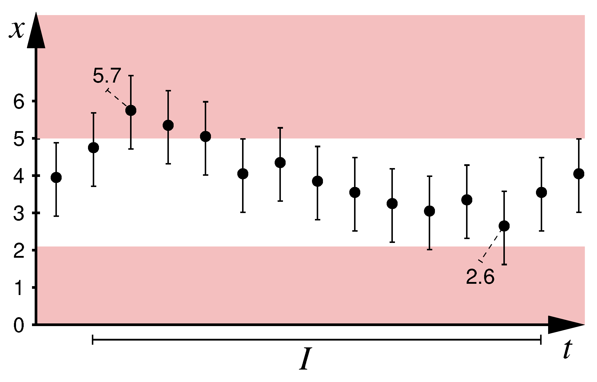
As a motivating example consider the time series of inexact measurements depicted in
Figure 1, where
t denotes time instant of the measurement (for simplicity considered to be exactly known and to coincide with the time of its associated ground truth values—both simplifications can be relaxed),
x is the unknown ground-truth value of the physical quantity x under observation,
black dots denote inexact measurements taken at time instances ,
perpendicular intervals attached to measurements indicate error margins: measurements may deviate by from ground truth; thereof can be attributed to an unknown constant sensor offset, leaving another to random measurement noise,
the red areas, corresponding to the state predicate , indicate critical values for x, e.g., a geo-fencing condition not to be violated,
the monitoring condition is to be decided at time for time , i.e., whether , avoiding the red range, holds throughout the depicted time interval I.
The uncertainty intervals depicted are tight insofar that, first, their width is
and thus coincides with the sum of the two errors sensor offset and random noise and, second, that in the absence of any known model of the system dynamics, no reach-set propagation across time instances is possible. Evaluation of
based on interval arithmetic [
12] therefore remains inconclusive, given that some uncertainty intervals (namely the ones at times
and
) overlap with the red areas, yet none falls completely into this forbidden range. As the intervals depicted represent the sharpest possible state estimates w.r.t. the metric error model discussed here, monitoring approaches based on first applying best-possible state estimation and subsequently evaluation of the monitoring condition are equally prone to remaining inconclusive.
Using affine arithmetic [
13] and SAT modulo theory solving over linear arithmetic (SMT-LA) [
14], we will, however, be able to decide that
is violated at time
. The core argument in the detailed, general construction to follow is that we can represent the possible ground truth values
relating to the measurements
as
with
representing the unknown, yet bounded sensor offset and
for
representing per-sample independent error. Now observe that
is unsatisfiable. The latter can be decided with SMT-LA solving. The unsatisfiability proves that at least one of
,
definitely falls into the red range due to the dependence introduced by the sensor offset.
For the full construction let us assume that
mentions the state variables ;
for each we are having a sensor with maximal offset and maximum random per-sample error ; (We will later relax the assumption that all variables in be directly observable through a sensor. To be meaningful, such partial observation does, however, require a system model permitting to infer information over unobservable variables, which is subject of the next section.)
that these sensors have provided measurements for each variable and each time instant . (We will likewise relax the assumption that each time point be observed by the sensors in the section to follow.)
We then build a linear constraint system, i.e., a Boolean combination of linear constraints as follows:
- 1.
For each
and each
, we declare a constant
- 2.
For each
, we declare a variable
of type real and generate the bound constraints
representing the sensor offset for measuring
v.
- 3.
For each
and each
, we declare a variable
of type real and generate the bound constraints
representing the per-sample independent error.
- 4.
For each
and each
, we declare a variable
of type real and generate a linear constraint
representing consistency between measurements and ground truth values as stated in Definition 3.
- 5.
Using standard constructions of SMT-based bounded model checking, we add an SMT-LA encoding for validity of at time to the constraint system as follows:
For each subformula of and each time instant we add a Boolean variable ,
if then we assert constraints stating that is invariantly true for each ,
if then we add constraints for each ,
if then we add to the constraint system for each ,
if then we add constraints for each ,
if
then we add constraints
for each
,
consequently is the root variable representing validity of at time .
- 6.
We finally add one of the two conjuncts
- (a)
or
- (b)
alternatively,
where , to the resultant constraint system and check both variants for their satisfiability using an SMT-LA solver.
Depending on the results of the two satisfiability checks, we report
if both systems are found to be satisfiable,
⊤ if the system (a) containing is unsatisfiable,
⊥ if the system (b) containing is unsatisfiable,
The resulting STL monitoring algorithm is best possible in that it is sound, conclusive, and complete:
Lemma 1. The above algorithm M constitutes an exact monitor in the sense of Definition 5.
Proof. In order to show that M is exact, we have to prove that it is complete, conclusive, and sound.
Completeness is straightforward, as the constraint system generated in steps 1 to 6 is finite. Its generation hence terminates, as do the subsequent satisfiability checks because SMT-LA is decidable.
For soundness and conclusiveness note that the constraint system generated by steps 1 to 4 constitute a Skolemized version of the equation (
1) defining consistency and that satisfiability of
(or of
alternatively) corresponds to invalidity of
(of
, resp.) with
. The subproblems decided within algorithm
M thus directly match the conditions used in Definition 5 to characterize soundness and being conclusive. □
Note that the above encoding can easily be adjusted to other metric error models beyond additive absolute error simply by changing the characteristic formula applied in step 4 and adjusting the bounds for the errors
and
accordingly. The relative per-sample error from Equation (
2) would, for example, be encoded by
. The subsequent SMT solving would then, however, require a constraint solver addressing a more general fragment of arithmetic than SMT-LA due to the bilinear term
.
6. Exact Monitoring under Imperfect Information Given Uncertain Linear Dynamics
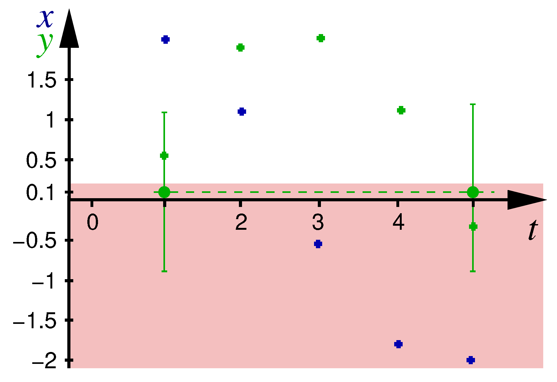
Additional inferences about the correlation between systems states at different time instants, and consequently additional evidence refining monitoring verdicts, are available when we have access to a model of system dynamics. Beyond refined arguments concerning feasible ground-truth value ranges within the error margins, such a model also allows to bridge gaps in sensor information, like time instants missing in a time series or references to unobservable signals. As a motivating example consider the time series of inexact measurements depicted in
Figure 2, where
t denotes time of measurement,
x and y constitute the (mostly unobservable) systems state, which is subject to uncertain linear dynamics and ,
blue (green, resp.) crosses denote the unknown actual values of x (y, resp.) along a system evolution,
green dots denote two inexact measurements taken on y at time instants 1 and 5, which are the only measurements available for the system,
perpendicular intervals of width denote the error margins of these measurements, consisting of independent per-measurement error and unknown constant sensor offset,
the red area indicates critical values for y, namely ,
the monitoring condition to be decided at for is , i.e., to decide whether the red area is avoided throughout time instants .
Evaluation of the monitoring condition over the uncertainty intervals remains inconclusive due to both the overlap of the given uncertainty intervals at times 1 and 5 with the red area and the lack of any information for the other times. Note that even most precise state estimation, while being able to deduce intervals for the possible ground truth values of y at time instants 2 to 4, cannot narrow down the intervals for y at time instants 1 and 5. Any monitoring approach based on a sequence of best-in-class state estimation and subsequent evaluation by a monitor thus is bound to remain inconclusive. Holistic treatment of the STL monitoring condition by affine arithmetic, however, can decide violation of the monitoring condition : the conjunction of the affine form representations of the relation between measurements and ground truth values with the equations for the system dynamics and with the monitoring condition constitutes an unsatisfiable linear constraint system (shown later in full detail).
The formal construction relies on the encoding from the previous section and conjoins it with the equations characterizing the system dynamics. It is generated as follows:
- 1–5
Identical to steps 1 to 5 from
Section 5, with the slight variation that constants representing measurements (step 1), slack variables for random noise (step 3) and constraints
encoding consistency with measurements (second half of step 4) are only generated for time instants where measurements are available.
- 6
For each
and each
, declare a real variable
and generate the linear constraints
when the dynamics of
v is given by the uncertain equation
. The uncertain offset
can be dropped when the dynamic equation is certain.
- 7
We finally add one of the two conjuncts
- (a)
or
- (b)
alternatively
to the resultant constraint system and check both variants for their satisfiability using an SMT-LA solver.
DECL
-- Ground-truth state variables
float [-100,100] x1, x2, x3, x4, x5;
float [-100,100] y1, y2, y3, y4, y5;
-- Actual measurements
define my1 = 0.1;
define my5 = 0.1;
-- Uncertainties in measurements
float [-0.5,0.5] oy, ey1, ey5;
-- Uncertainties in system dynamics
float [-0.1,0.1] uy1, uy2, uy3, uy4;
-- Helper variables for BMC encoding
boole p1, p2, p3, p4, p5, q1;
define s = 0.707106781; -- 1/sqrt(2)
EXPR
-- Uncertain linear system dynamics
x2 = s*x1 - s*y1;
y2 = s*x1 + s*y1 + uy1;
x3 = s*x2 - s*y2;
y3 = s*x2 + s*y2 + uy2;
x4 = s*x3 - s*y3;
y4 = s*x3 + s*y3 + uy3;
x5 = s*x4 - s*y4;
y5 = s*x4 + s*y4 + uy4;
-- Relations between measurements and states
-- reflecting an absolute error of +-0.5 both as offset and random
y1 + 0.5*oy + 0.5*ey1 = my1;
y5 + 0.5*oy + 0.5*ey5 = my5;
-- BMC encoding of monitoring condition
-- p_ represents satisfaction of y >= 0.2 at time instant _
p1 <-> y1 >= 0.2;
p2 <-> y2 >= 0.2;
p3 <-> y3 >= 0.2;
p4 <-> y4 >= 0.2;
p5 <-> y5 >= 0.2;
-- q_ represents validity of G <=5 p at time instant _
q1 <-> p1 and p2 and p3 and p4 and p5;
-- Goal, namely satisfaction of q at time 1
q1;
Note that the above encoding employs the slightly optimized BMC encoding
for subformulae
at each
.
The above constraint system is unsatisfiable, confirming the verdict ⊥ for the monitoring condition
at time
. Its unsatisfiability can automatically be decided by any satisfiability modula theory (SMT) solver addressing SMT-LA, i.e., Boolean combinations of linear inequalities. Likewise, its variant encoding the relative error model from Equation (
2) can be decided by any SMT solver solving Boolean combinations of polynomial constraints. Such solvers do in general rely on solving a Boolean abstraction of the SMT formula, where all theory atoms (linear or polynomial inequalities in our case) are replaced by Boolean literals by a CDCL (conflict-driven clause learning) propositional satisfiablity (SAT) solver [
22,
23] in order to resolve the Boolean structure. As this SAT solving incrementally instantiates the Boolean literals in the abstraction, a conjunctive constraints system in the theory underlying the SMT problem (e.g., linear arithmetic) is incrementally built by collecting the theory constraints that have been abbreviated by the Boolean literals. These conjunctive systems of theory constraints are then solved by a subordinate theory solver, which blocks further expansion of the partial truth assignment to the literals in the Boolean abstraction when the associated theory-related constraint system becomes unsatisfiable. The reasons for unsatisfiability are usually reported back to the SAT solver in form of a corresponding conflict clause over the abstracting Boolean literals, where the conflict clause reflects a minimal (or, in cases of undecidability of high computational cost, small) infeasible core of the unsatisfiable theory constraint system. This conflict clause is added to the Boolean SAT problem and forces the SAT solver into (usually non-chronological) backtracking, thus searching for a different resolution of the Boolean structure of the SMT problem. A thorough description of the algorithmic principles underlying this so-called lazy theorem proving approach to SMT can be found in [
24,
25]. iSAT is an industrial-strength SMT solver that is commercially available [
26] and covers a very general fragment of arithmetic, covering linear, polynomial, and transcendental functions over the integers, the mathematical reals, and (in bit-precise form) the computational floats [
27].
Although iSAT [
21,
28,
29] is by no means optimized for solving linear constraint systems—its primary field is non-linear arithmetic involving transcendental functions, the above monitoring condition can be checked in approximately 300 ms on a single core of a Core i7 10th generation running at 1.8 to 2.4 GHz. iSAT would, with essentially unaltered performance, be able to also check error models whose encoding requires non-linear arithmetic, like the mixed absolute-relative error model of Equation (
2). In the above case of absolute error, we may equally well apply the dedicated SMT-LA solver MathSAT 5 [
15] to the equivalent SMT-lib encoding shown in
Appendix A, as only linear arithmetic is involved. The runtime then amounts to just 9.4 ms on an eight-core AMD Ryzen 7 5800X running at 4.4 GHz. As these runtimes have been observed on general-purpose SMT solvers devoid of any particular optimization for the formula structures arising in the monitoring problem, we deem online monitoring in real-time practical even for more complex (deeper nesting of sub-formulae, larger
) monitoring conditions and system models (higher dimensionality especially), given the proven scalability of SMT to large-scale industrial problems.
For the above model-based monitoring procedure, akin to Lemma 1, we obtain
Lemma 2. For systems featuring uncertain affine dynamics, the above monitoring algorithm is exact, where exactness in this setting refers to exact characterization, in the sense of Definition 5, of the truth values possible over with D being the set of possible trajectories of the system according to its uncertain linear dynamics.
8. Conclusions
In this article we have shown that the monitoring under uncertain environmental observation of properties expressed in linear-time temporal logic is fundamentally different from state estimation under uncertainty. While accurate state estimation followed by evaluation of the monitoring property provides a sound mechanism, this two-step algorithm may remain unnecessarily inconclusive. We have exposed two sample cases where a direct evaluation of the temporal logic property, for which we gave the formal constructions via a reduction to SAT modulo theory solving over linear arithmetic, yields definite results, whereas the two-step algorithm based on state estimation remains inconclusive. The reason is that durational properties expressed by temporal logic induce rather complex relations between successive values of signals and that these relations overlap and interfere with the cross-measurement relations induced by measurements of dynamically related variables as well as by dependencies between measurements. The single-step reduction exposed in this article encodes both the specification formula to be monitored and the error model for measurements into a common logical representation such that the interaction between these two cross-time-instant relations can be analyzed and exploited for more informed verdicts.
In the present article, we have analyzed these effects theoretically and on small, prototypic examples, within a setting of non-stochastic, metrically constrained error, where the different types of measurement error are interval-bounded. Future work will address real-life benchmark applications from the air taxi domain and extend the theory to a stochastic setting, where both measurement errors and uncertain system dynamics are described by distributions rather than metric intervals. Furthermore, we will address run-time efficiency by devising structural SMT approaches exploiting the particular problem structure rather than using problem-agnostic general purpose SMT solvers. Where this does not suffice to obtain real-time capabilities suitable for online monitoring, we will reduce computational complexity by appropriate approximation algorithms providing real-time capabilities in settings where the exact reductions and the SAT modulo theory algorithms used herein do not feature sufficient performance.
A further issue of interest could be the handling of outliers in the measured time series, where tolerance of the monitoring verdict against
outliers would constitute a useful relaxation of the monitoring requirement. In such a relaxation, a monitor alarm would be suppressed if, at most,
k measurements can be replaced by (arbitrarily different or bounded-offset) valuations that render the monitoring condition true when combined with the ground-truth of the remaining noisy measurements. Such tolerance against a fixed number of outliers can well be encoded and solved via SMT, as has been demonstrated in [
31].


