Apple Shape Detection Based on Geometric and Radiometric Features Using a LiDAR Laser Scanner


1
Department Horticultural Engineering, Leibniz Institute for Agricultural Engineering and Bioeconomy (ATB), Max-Eyth-Allee, 14469 Potsdam, Germany
2
Department of Natural Resources Management and Agricultural Engineering, Agricultural University of Athens, 11855 Athens, Greece
3
Institute of Agricultural Engineering, Technology in Crop Production, University of Hohenheim, Garbenstraße 9, 70599 Stuttgart, Germany
*
Author to whom correspondence should be addressed.
Remote Sens. 2020, 12(15), 2481; https://doi.org/10.3390/rs12152481
Submission received: 14 June 2020
/
Revised: 25 July 2020
/
Accepted: 31 July 2020
/
Published: 3 August 2020
(This article belongs to the Section Remote Sensing in Agriculture and Vegetation)
Abstract
:Yield monitoring systems in fruit production mostly rely on color features, making the discrimination of fruits challenging due to varying light conditions. The implementation of geometric and radiometric features in three-dimensional space (3D) analysis can alleviate such difficulties improving the fruit detection. In this study, a light detection and range (LiDAR) system was used to scan apple trees before (TL) and after defoliation (TD) four times during seasonal tree growth. An apple detection method based on calibrated apparent backscattered reflectance intensity (RToF) and geometric features, capturing linearity (L) and curvature (C) derived from the LiDAR 3D point cloud, is proposed. The iterative discretion of apple class from leaves and woody parts was obtained at RToF > 76.1%, L < 15.5%, and C > 73.2%. The position of fruit centers in TL and in TD was compared, showing a root mean square error (RMSE) of 5.7%. The diameter of apples estimated from the foliated trees was related to the reference values based on the perimeter of the fruits, revealing an adjusted coefficient of determination (R2adj) of 0.95 and RMSE of 9.5% at DAFB120. When comparing the results obtained on foliated and defoliated tree’s data, the estimated number of fruit’s on foliated trees at DAFB42, DAFB70, DAFB104, and DAFB120 88.6%, 85.4%, 88.5%, and 94.8% of the ground truth values, respectively. The algorithm resulted in maximum values of 88.2% precision, 91.0% recall, and 89.5 F1 score at DAFB120. The results point to the high capacity of LiDAR variables [RToF, C, L] to localize fruit and estimate its size by means of remote sensing.

1. Introduction
In the quest of decreasing farming costs and increasing sustainability, leaf area and yield monitoring are considered as one of the most important steps when implementing precision agriculture technologies in orchards [1,2]. Monitoring of leaf area index and yield has been widely studied and applied in cereal crops such as rice [3], sorghum [4], wheat [5], maize [6]. Similarly, in orchards the monitoring of tree morphology and growth is requested, since the variation in the leaf area and resulting light interception influences the fruit-bearing capacity of the tree. Furthermore, the shading of fruit affects the fruit color, which is an important parameter of fruit quality [7]. However, the coinciding structures and the varying reflectance properties of the tree organs work as suspending factor for yield mapping systems, particularly making the automated fruit detection challenging.
The localization of fruit and estimation of fruit size have gradually gained an essential driving force by the emerging implementation of robotics in agriculture [8]. Various machine vision systems have been developed based on color, spectral, and thermal imaging. Color, extracted from two-dimensional RGB images, was utilized as an indicative factor of fruit detection in apple [9,10], citrus [11,12], mango [13], and grapes [14]. However, the captured images are sensitive to light variation, while the detection can be biased in cases of equal color of fruit, leaves and branches [15,16]. Thus, the RGB images were frequently fused with thermal images to overcome this issue, e.g., in green apples [17] or green citrus [18]. Due to increased spectral resolution compared to RGB imaging, spectral imaging can potentially be utilized for fruit detection based on the reflectance intensity altered by the fruit pigments [19] by means of either multispectral [20,21] or hyperspectral cameras [22,23]. However, varying lighting conditions remain a perturbing factor.
The recent advancements in three-dimensional (3D) remote sensing technologies received attention in agriculture, enabling potential prospects to overcome the limitations of 2D imaging methods [24]. The 3D point cloud data can restore the shape of fruit trees, providing highly resolved spatial data for fruit localization. Besides the triangulation techniques, which allow the acquisition of 3D information from stereo vision or structured light cameras, 3D point cloud data and radiometric information can be generated by RGB depth (RGB-D) cameras, which operate based on stereo vision or time-of-flight (ToF) measuring principle. The latter RGB-D sensor captures three different modalities: color, depth, and the backscattered reflectance intensity (RD) at the wavelength of an integrated ToF depth sensor. By means of these data providing geometric (depth) and radiometric (RGB and RD) information, the discrimination potential of fruit from foliage and woody parts of the plant are assumed to be enhanced. Gene-Mola et al. [25] used range corrected data capturing color, depth, and RD in the near-infrared wavelength range from an RGB-D camera to detect the apple shape at the tree, resulting in 0.89 F1-score and 94.8% average precision. The authors pointed out that the depth and RD provided the most robust variables in the calibration model, while RGB was highly influenced by light shading in the canopy. In mango, RGB-D imaging enabled to detect mangoes with 81% precision, and to estimate the length and width of the fruit, achieving a root mean square error (RMSE) of 4.9 mm and 4.3 mm, respectively [26]. Both studies were undertaken after sunset to achieve consistent lighting conditions. It was noticed that the sensor failed to acquire distance information over 3.5 m. Another technique for acquiring 3D information are the light detection and ranging (LiDAR) laser scanners, which are operated based on the ToF principle with a scanning mechanic for obtaining advanced high-density spatial resolution compared to RGB-D sensing. The data acquired are the laser hits based on ToF principle providing geometric information and optionally the intensity of reflected, apparently backscattered, laser hits gaining radiometric information.
Currently, LiDAR intensity data were applied for feature extraction, classification, and object detection and recognition on natural and urban surfaces [27]. In fruit production, working in a 3D space allows the identification of geometric tree features such as the shape and size aiming the fruit localization [28]. The spatial distribution of the geometric features can be illustrated by the decomposition of the covariance matrix from a set of points in 3D. Brodu and Lague [29] proposed that the set of points within the spherical neighborhood can be utilized to define whether the geometric structure of points is closer to a line, plane surface, or a random cluster. Several researchers in forestry applications used the method to include reflectance intensity (RToF) and geometric features such as the linearity to discriminate foliage from woody parts [30,31] or to estimate the leaf angle [32]. Whereas in agriculture, Gene-Mola et al. [33] proposed a methodology that combines the backscattered reflectance intensity and a geometric factor for spherical shapes based on the eigenvalues of clusters in apple trees to localize the fruits. The method gained 87.5% localization success, 82.4% identification success, and a F1-score of 0.86 in relation to the total number of fruits. Moreover, eigenvalues of geometric data on curvature and linearity have been computed to distinguish cotton balls from branches, reaching 90% detection accuracy [34]. Similarly, intensity and geometric features have been exploited to train harvesting robots in greenhouse applications [35,36].
The aim of this study is to propose a methodology for segmenting, localizing, and analyzing fruit on the tree, based on the assumption that apples show enhanced RToF at 905 nm compared to foliage and woody parts. The main objectives are: (1) the classification of 3D points of apples based on reflectance and geometric features derived from LiDAR laser scanner; (2) the development of a fruit segmentation algorithm that allows measuring the fruit size in defoliated trees; and (3) the evaluation of the proposed technique on foliated apple trees at different growth stages.
2. Materials and Methods
2.1. Site Description
The study was carried out in the experimental station Field Lab for Digital Agriculture by Leibniz Institute of Agricultural Engineering and Bioeconomy (ATB) located in Marquardt, Germany (Latitude: 52.466° N, Longitude: 12.958° E) during the growing season 2019. The trees of Malus × domestica Borkh. ‘Gala’ on M9 rootstock were planted in a 0.37 ha orchard, 0.95 m within-row distance between trees, which have been trained as tall slender spindle (central leader) formation with 3.3 m maximum tree height. The trees were supported by utilizing four horizontally parallel wires (W1, W2, W3, W4) with 1 m equal distance from each other. Plants were drip irrigated, fertilized, and treated according to management in commercial orchards and the regional plant protection plan. Hand thinning resulted in 1–3 fruits per inflorescence.
2.2. Data Acquisition and Pre-Processing
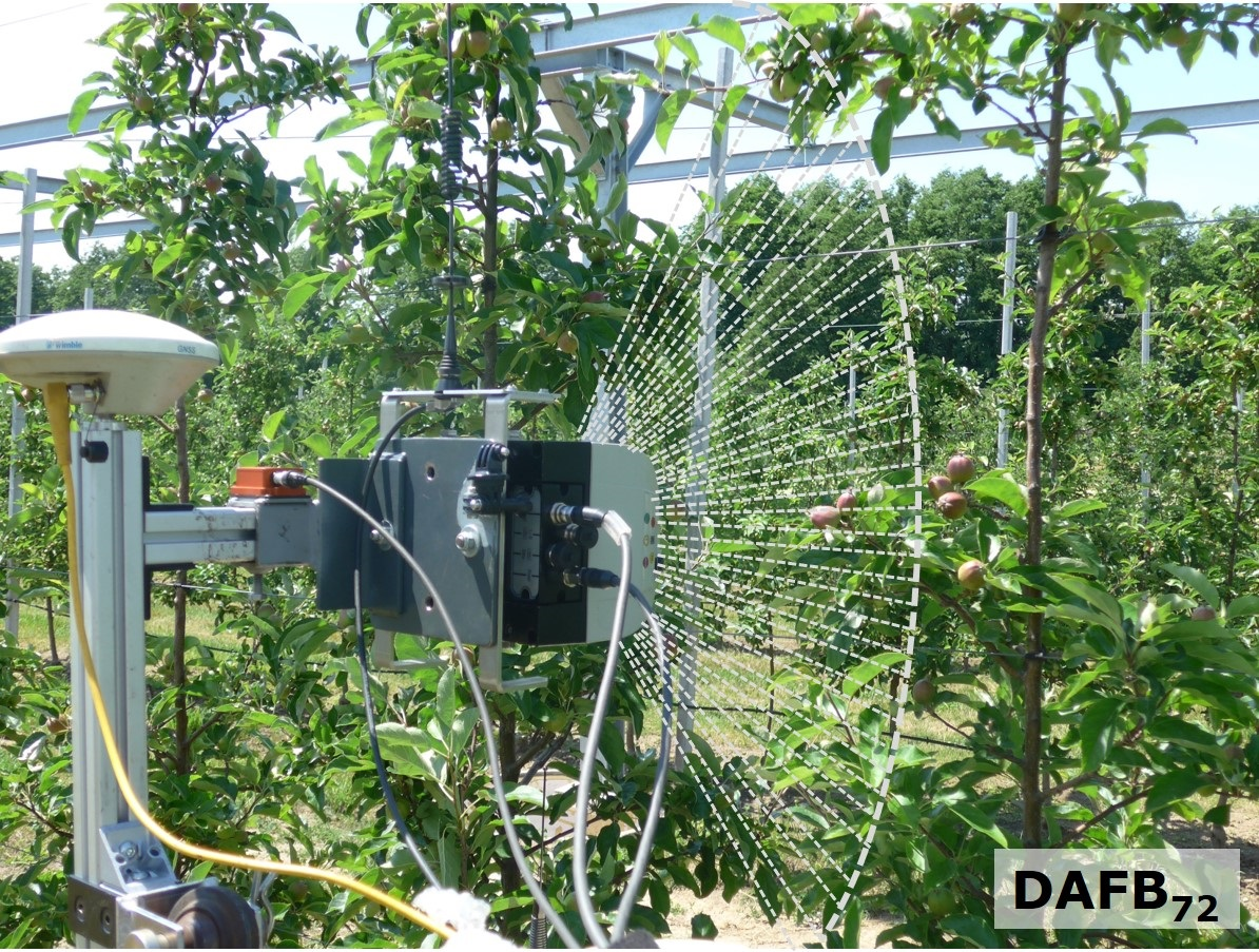
A metal frame installed on a tractor was used to carry the sensors along the tree rows [37]. A mobile terrestrial LiDAR laser scanner (LMS-511, Sick AG, Waldkirch, Germany) was mounted vertically on the metal frame at 1.6 m above the ground level.
The LiDAR sensor was configured with a 0.1667° angular resolution, 25 Hz scanning frequency and a scanning angle of 190°. The sensor frame was driven along the rows on both sides of the trees with an average speed of 0.13 m s−1. The measured objects, hit by the laser beam, were assumed as perfectly diffuse reflectors (Lambertian), excluding the influence of incidence angle [38,39]. Thus, the apparent signal was considered as an approximation of hemispherical reflectance. Board targets, coated with white barium sulphate (BaSO4, CAS Number: 7727-43-7, Merck, Germany) for maximum (Rmax) and blackened urethane (S black, Avian Technologies, New London, NH, USA) for minimum (Rmin) referencing were applied to calibrate the backscattered intensity (RToF) of the LiDAR, obtaining the RToF [%] at 905 nm for each point in the 3D point cloud (Equation (1)).
The tractor movement was recorded by an inertial measurement unit (IMU) (MTi-G-710, XSENS, Enschede, the Netherlands), allowing the correction of errors due to the uneven ground surface. The root mean square error (RMSE) of orientation noted at 0.25° for roll, pitch and yaw [40]. Furthermore, a RTK-GNSS (AgGPS 542, Trimble, Sunnyvale, CA, USA) was used for georeferencing each individual point of the 3D point cloud. The horizontal and vertical accuracy of the RTK-GNSS was ± 25 mm + 2 ppm and ± 37 mm + 2 ppm, respectively. The IMU was place 0.24 cm aside from the LiDAR sensor, while the receiver antenna of RTK-GNSS was mounted 0.30 cm above the laser scanner (Figure 1). A multi-thread software was developed in Visual Studio (version 16.1, Microsoft, Redmond, WA, USA) to acquire the data [37].
The 3D point cloud data was processed in the Computer Vision Toolbox™ of Matlab (2017b, Mathworks, Natick, MA, USA). A sparse outlier removal was applied to each point cloud pair to reject the points that were above the average distance using CloudCompare (2.10, GPL software, Paris, France). Moreover, the random consensus was performed to filter the points that belonged to the ground [41]. According to Tsoulias et al. [37], the rigid translations and rotations were applied in each point of the point cloud, while the alignment of the pair tree sides was carried out with the iterative closest point algorithm, using a k-dimensional space to speed up the process.
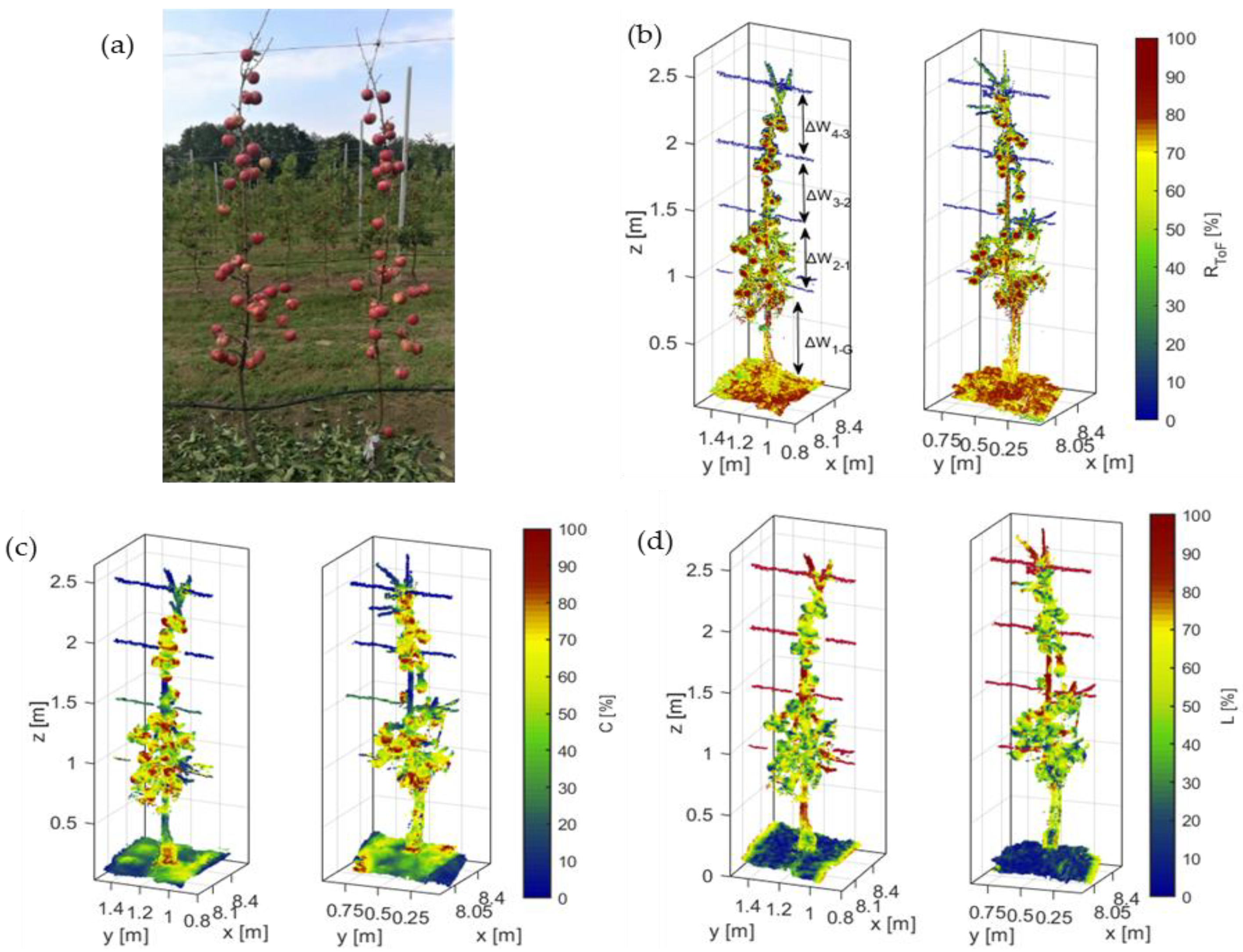
Data were recorded during fruit growth starting when the end of the cell division stage of fruit was reached and the cultivar-typical red blush color [42] appeared and on subsequent three dates, i.e., 42, 72, 104, and 120 days after full bloom (DAFB42, DAFB72, DAFB104, DAFB120, respectively). On each measuring date two apple trees (n = 8) were initially scanned with leaves (TL), while the measurement was repeated with the plants defoliated (TD). After scanning, the total number of apples was counted on the tree. After harvest, fruit’s diameter (DManual) was manually measured in the lab. All apples of each tree were categorized according to their growing position on the slender spindle. The wires (W) were used as borders to discriminate the apples between the ground and W1 (ΔW1-G); W1 and W2 (ΔW2-1); W2 and W3 (ΔW3-2); W3 and W4 (ΔW4-3).
2.3. Apple Detection Methodology
2.3.1. Extraction of Radiometric and Geometric Features
The information of the 3D local neighbourhood of points = [] was determined using the k-nearest neighbours within a radius (r) equal to the mean DManual of apples [43]. The total number of the data set (K) was used to estimate the average = of the nearest neighbours. Thus, the covariance matrix (Cov) was built after mean centering by means of subtraction of value from each of the nearest neighbours set (Equation (2)):
The Cov was decomposed based on the singular value decomposition, producing the eigenvalues (, , ), which were sorted in ascending order ≥ ≥ according to the variance captured, and the corresponding eigenvectors. The eigenvalues, which represent the highest orthogonal variance of the matrix, provided the points dispersion within k-nearest neighbours describing the local spatial structure in 3D. The eigenvalues were scaled between 0 and 100, allowing the comparison of different clusters. Thus, the local geometry of each Pi in the point cloud was analyzed by means of eigenvalues to illustrate the spatial structure considering its linearity (L, Equation (3)) and curvature (C, Equation (4)):
where L and C describe the variation of linearity and curvatures for all points along the direction of the corresponding eigenvalues, respectively [43,44]. More specifically, the closer the values of L or C to 100, the higher the likelihood for the shape of points to be linear or curved, respectively. Therefore, L was used to segment the foliage and woody parts of the tree (leaves, branches, stem), while C was applied to distinguish the apple points.
2.3.2. Apple Segmentation
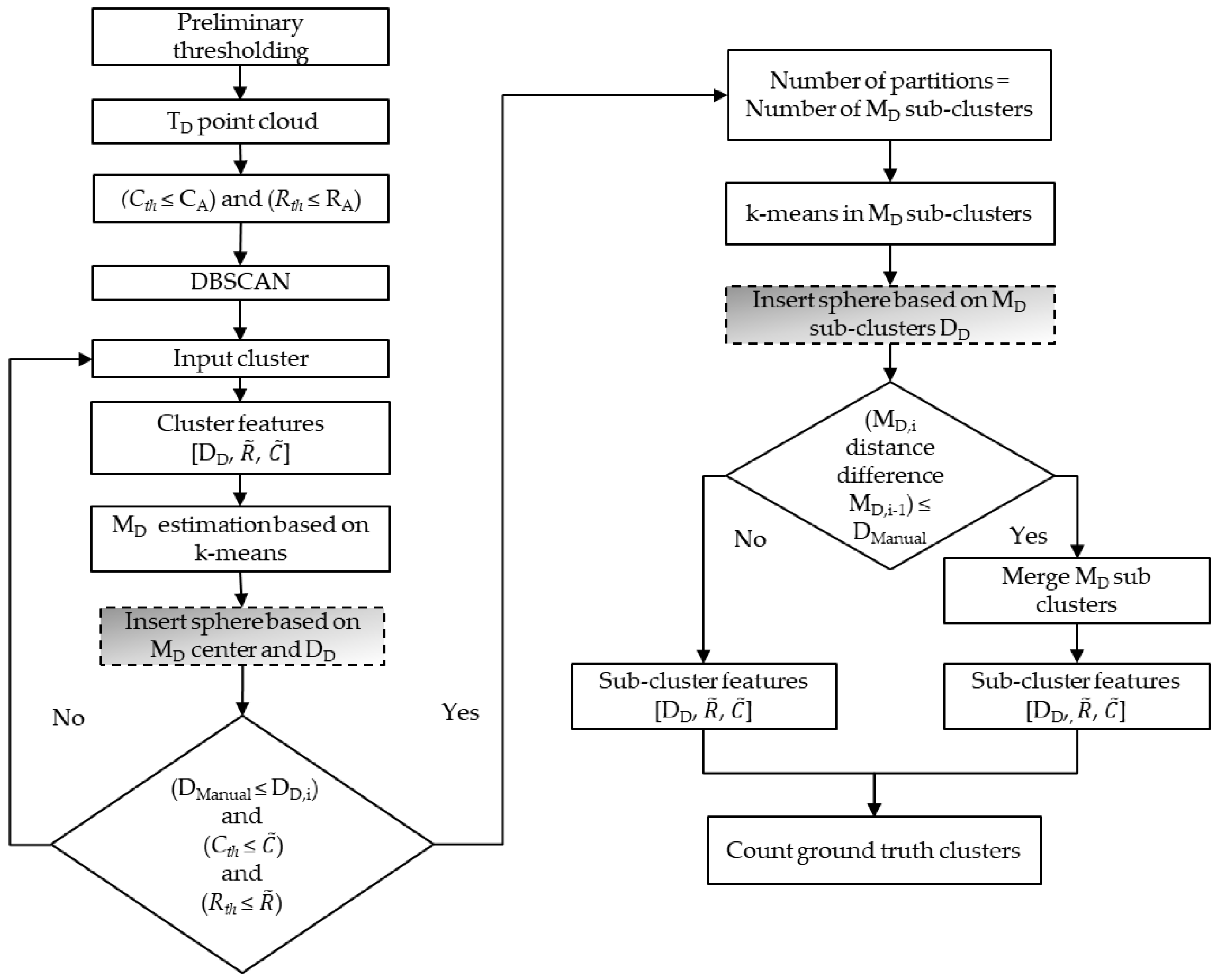
The data set of TD at DAFB120 (n = 2) was used to define the range of RToF, C and L for the class of apple (RA, CA, LA) and of woody parts (RW, CW, LW), while the range of leaf class for the same features (RL, CL, LL) was defined in the TL. The thresholding was performed for each class by employing the exploratory analysis of normal distribution using the probability density function to define the threshold that will distinguish the 3D points of apples from leaves and woody parts [33,45]. The value with the highest likelihood (mode) within the RA, CA, and LA classes was used as a threshold (Rth, Cth, and Lth). Points which fulfilled the criteria of LA ≤ Lth, Cth ≤ CA, and Rth ≤ RA were segmented and categorized as apples. Figure 1 represents a flowchart of the protocol for apple detection and sizing using the defoliated trees (TD).
Subsequently, a density-based scan algorithm (DBSCAN) [46] was applied to find the point sets, using the mean DManual of apples that was found in each ΔW as a neighborhood search radius (ε) and the value 10 as a minimum number of neighbors. The value of 10 was applied resulting from manually run tests showing that less neighboring points result in random appearance of sets. The mean value of apparent reflectance intensity and of curvature in defoliated trees ( and ) were calculated to classify the clusters. The maximum distance in x and y axes was considered as the diameter (DD) of each point set recognized as an apple.
Following, the k-means clustering was applied to count and find the fruit center (MD) in each cluster in TD. However, the shape variation of each apple and the clustering of more than one apple produced different C and RToF. Consequently, the utilization of Cth and Rth values possibly exclude points at the edge of the fruit. Therefore, a sphere was placed in each individual apple cluster, with the coordinates of MD as the center and a radius equal with the estimated DD to include the filtered apple points. The k-means algorithm was reapplied to estimate the MD of each cluster based on the added 3D points, while the and were recalculated.
The fact that more than one apple developed per inflorescence led to close appearance of 2–3 fruits in the cloud, resulting in the creation of augmented clusters with more than one apple. Thus, the clusters of 3D points within the sphere were evaluated and partitioned based on their extracted features, creating sub-clusters and defining the number of MD. Therefore, the partitioning was performed for each cluster only on the condition that the three variables, DD, , and , were close to mean values of DManual measured at DAFB120 for each ΔW and Rth, Cth. The features of each sub-cluster were iteratively extracted and re-evaluated, while the partitioning was continued until the sub-cluster features stopped, while fulfilling the condition. Subsequently, the spheres were placed based on the MD and the DD of each sub-cluster. Those spheres, showing a calculated distance between the MD centers below the minimum value of DManual in each ΔW, were merged. Therefore, their MD was redefined and their extracted features were recalculated. It should be mentioned that the MD clusters were considered as ground truth labels for the later evaluation of the method in TL.
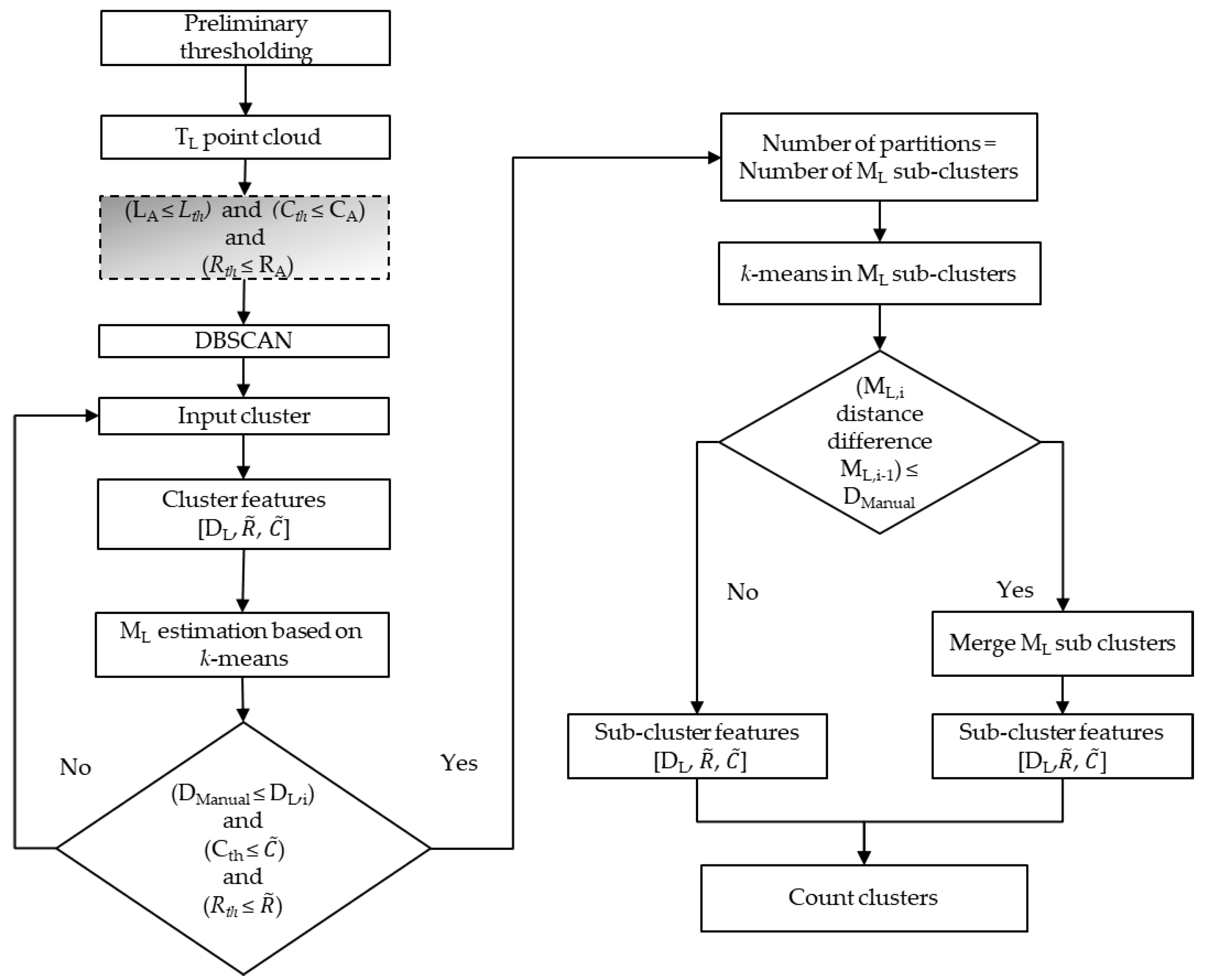
Similarly, the Lth, Cth, Rth were applied to the same trees before their defoliation to segment the apples and find their centers (ML) (Figure 2). The DBSCAN was used to group the segmented points, while the ML centers were defined by the k-means algorithm. Furthermore, the maximum distance in x and y axes was considered as the diameter (DL) of each point set. The main partitioning condition remained the same using the generated features from each cluster. Thus, the features of each TL sub-cluster were iteratively extracted and re-evaluated until fulfilling the conditions. The number of partitions was used in the k-means algorithm to determine the centers of ML sub-clusters. The only difference between analysing TD and TL was the use of the sphere in TD to evaluate the eligibility of the cluster or the need to search for subclusters according to the estimated manually measured fruit diameter.
However, in TL, some of the apples were fully or partially covered by the leaves of the tree. In the latter case, the combination of DBSCAN and k-means algorithm overestimated the number of apple classes. Thus, apple classes producing lower or equal Euclidian distance between their ML centers compared to the minimum DManual were combined and considered as one fruit.
2.4. Evaluation
The calibration of the method was carried out considering data from TD and TL at DAFB120 (n = 2) to define the Rth, Cth and Lth that describe the apple class. Cross-validation, applying thresholds extracted at DAFB120, was performed to the TD and TL data sets of the three earlier measuring dates (n = 6). The fruit detection methodology was evaluated by calculating the accuracy, the precision, the recall, and the F1 score:
The MD were considered as ground truth labels for the evaluation of ML. The ML clusters which coincide with the MD points >50% were considered as true positive (TP). The true negative (TN) refers to the situation when a cluster was correctly categorized as no fruit. Whereas the ML clusters which matched <50% were counted as false negative (FN). The clusters which reveal a diameter smaller than the minimum value of DManual that was found in each ΔW were categorized as false positives (FP). N denotes the sum of TP, TN, FP and FN. The values were given as percentage.
A regression analysis was performed between the DManual and the DD, and RMSE, mean absolute error (MAE), mean bias error (MBE) were calculated for each measuring date. The position of each ML was evaluated with the MD using the Euclidean distance, pairing the centers that revealed the minimum distance between them. In parallel, the difference between the fruit diameter in TD and TL was estimated, considering the DD as ground truth for DL.
3. Results
3.1. Apple Segmentation
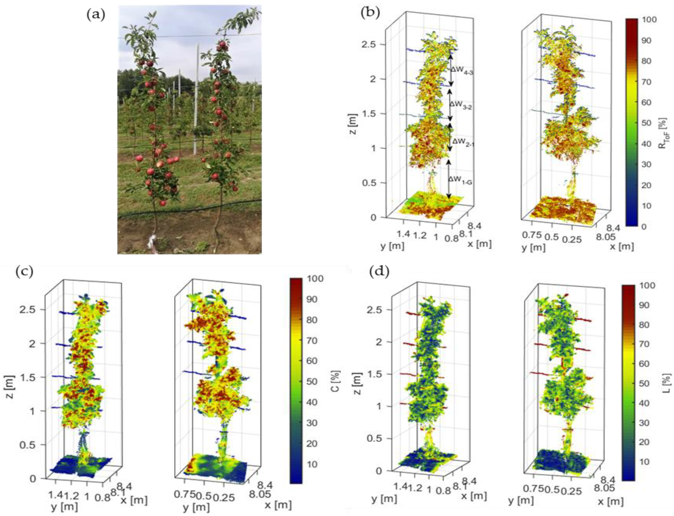
The definition of apple class was carried out on the data set of last day’s measurements at DAFB120. The calibrated reflectance intensity RToF varied in the 3D point cloud of the foliated trees (Figure 3b). The RToF values of apples (RA) and woody parts (RW) appeared above 70% and below 55%, respectively. The leaves (RL) ranged between 40 and 80%. The C values of leaves (CL) ranged between 35.2% and 70% (Figure 3c). The C values of apples (CA) were observed above 50%, whereas the points of woody parts (CW) did not exceed 60%. The L of leaves (LL) ranged between 20% and 80%, while the woody parts (LW) were scored above 60% (Figure 3d).
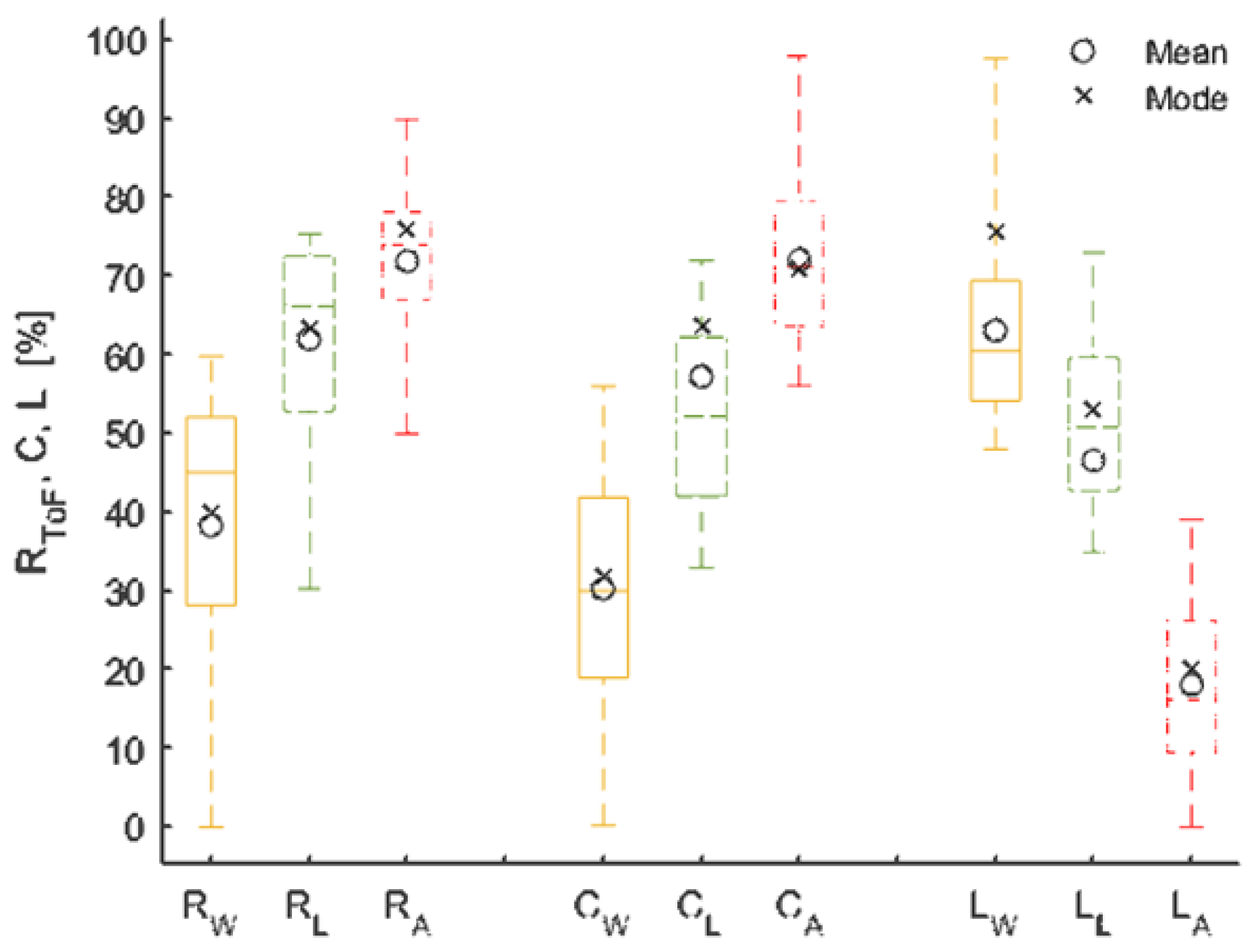
However, the occlusions of leaves and woody parts did not allow the acquisition of the full range of RToF, C, and L values of apples. Therefore, the trees were defoliated and scanned with the LiDAR system at DAFB120 (Figure 4) and data were used to readjust the thresholds. The RW values ranged between 0 and 60%, while the RA appeared from 42 to 90% (Figure 4b). The CA values of apples ranged between 56 and 98%, and the CW appeared between 0.1 and 55.2% (Figure 4c). The 3D points of the latter category revealed the highest values varying between 48.8 and 98.8%. The L values of apple points (LA) were more discretely ranging between 0.2 and 38.3%. (Figure 4d). However, the highest mean value was obtained from the RA class at 71.8%, whereas the mode value (76.1%) was utilized as Rth for the ‘Gala’ trees.
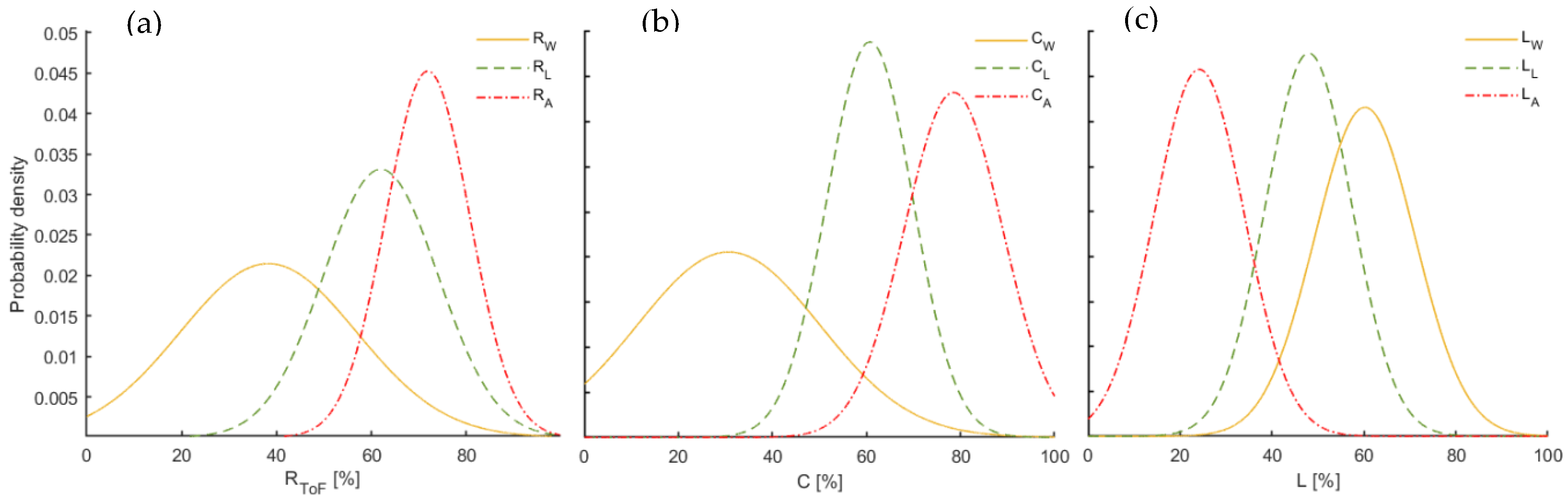
As mentioned above, the RToF values of apples could overlap with the leaves or the woody parts, while some of the surfaces may reveal similar C with apples, producing falsely clusters from leaves or woody parts. The RW showed a mean value of 38.2% with standard deviation (SD) of 18.5%. In contrast, the RToF of leaves (RL) and of apples (RA) were marginally deviated (Figure 5a), while most of their values appeared from 50 to 70% and from 65 to 71.8%, respectively. More specifically, the mean value of RL was indicated at 58.8% with 12.1% SD, and 63.2% as the value with the highest likelihood (mode) within the class.
A similar pattern of the probability density of RToF was obtained in C (Figure 5b). The most frequent value within the CA was illustrated at 73.2% (Cth). The values of C of leaves (CL) were partly coinciding with the CA, revealing a mean value at 60.7%, and 9.1% SD. The CW revealed a mean value of 30.1%, with 19.4% SD. The 3D points of LW depicted the highest values (Figure 5c), reaching a mean value of 60.2%, and 94.1% as mode value (Figure 6).
The RA, CA and LA values were distinct from the residual classes, allowing the discrimination and localization of apples in the 3D point cloud. The apples were described with RA and CA values 76.1% and 73.2% (Figure 6). Therefore, the Rth and Cth were combined and used as thresholds to distinguish the apple points from woody parts. Whereas the remaining points of the latter class were removed using the LW mode value of 15.5% as threshold (Lth) (Figure 6).
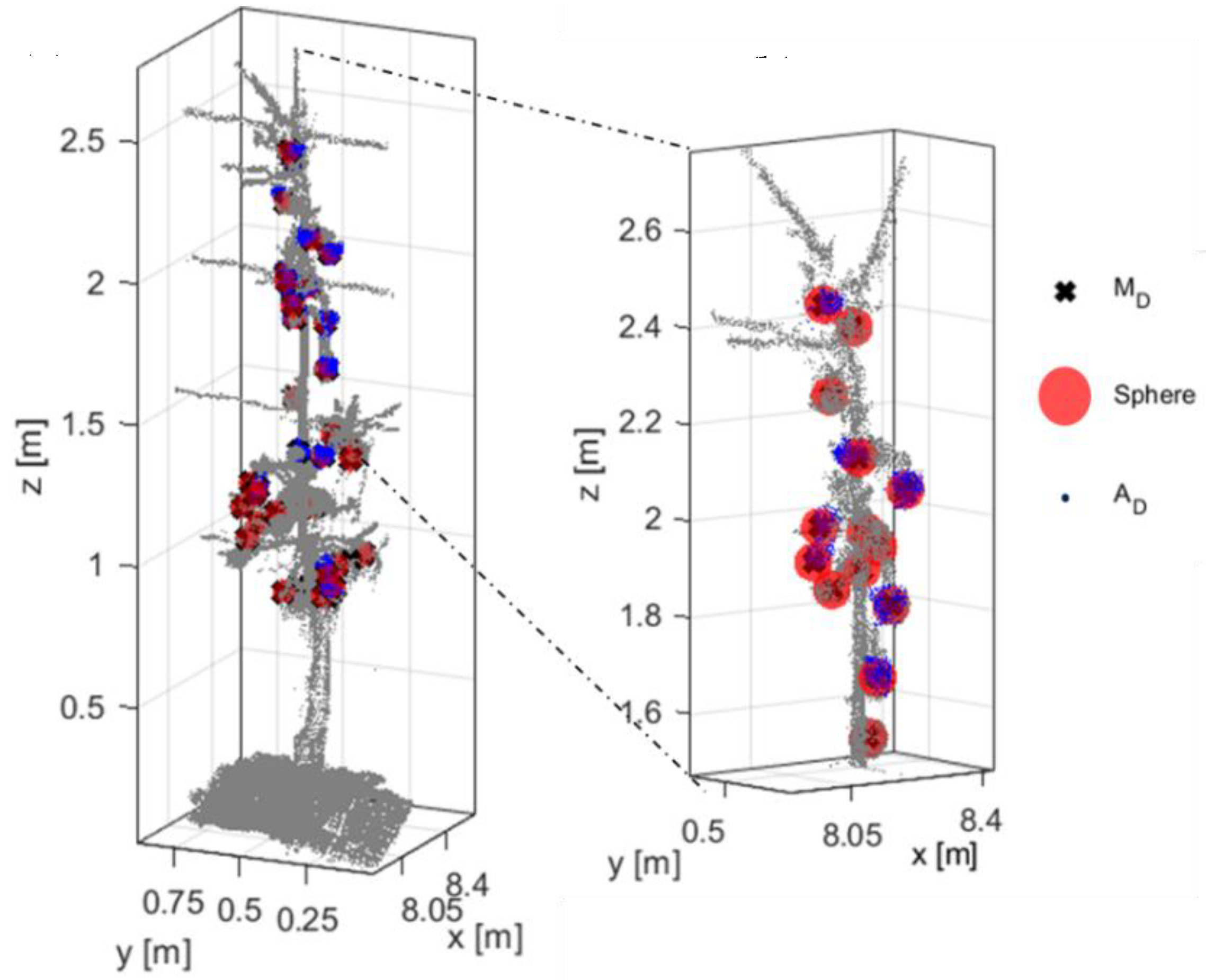
When performing the DBSCAN algorithm, the clusters of filtered points of apples appeared in the 3D point cloud (Figure 7). Subsequently, the k-means partition method was applied to the points of each cluster to acquire the MD. A sphere of variable radius based on the DD of the cluster, enclosed the points of the cluster when placed at MD.
After the localization of MD, the estimated fruit diameter, DD, was compared to the DManual for each ΔW during the growth stages (Table 1). The DD was related to the DManual. In the upper sections, ΔW3-2 and ΔW4-3 of the canopies, where the fruit grow more distinctly, the analysis of apple size resulted in an adjacent coefficient of determination (R2adj) of 0.69 and 0.74 with RMSE = 7.2 and 6.6% at DAFB42, respectively. Generally, high measuring uncertainty was noticed on the first two measuring dates, when the fruit size was smaller, particularly in the lower sections of the trees with overlapping structures. More specifically, no relation was observed on the first measuring date in ΔW1-G and ΔW2-1, presenting an overestimation of 6.5 mm and 7.5 mm, respectively. Similarly, at DAFB72 in the same areas, the MBE points to an underestimation of fruit diameter of −10.7 mm and −9.11 mm. In contrast, the highest relation was revealed in ΔW4-3 (R2adj = 0.95) and ΔW3-2 (R2adj = 0.90), at DAFB104. Whereas, in the same stage, a less pronounced R2adj was observed in ΔW1-G (R2adj = 0.55) and ΔW2-1 (R2adj = 0.66) compared to the aforementioned upper zones of the trees. The measuring uncertainty was slightly enhanced again at DAFB120. The crop load of trees usually varies between the trees, affecting the fruit size. The high crop load of the trees analysed at DAFB120 resulted in slightly smaller fruit size compared to trees with lower crop load sampled at DAFB104. Consequently, the method showed lowest measuring uncertainty in the biggest fruit at DAFB104 considering the defoliated trees.
3.2. Evaluation
In foliated trees, TL, the same procedure was followed applying the same threshold values gained in the calibration on the data set obtained at DAFB120. For evaluating the performance of the segmentation process in foliated trees, TL, the data set of defoliated trees TD was employed as ground truth. For this purpose, the ML clusters found in TL were compared to the clusters, MD, found in TD.
The total number of the apple clusters in defoliated trees (nD) was 42 in ΔW1-G, 84 in ΔW2-1, 91 in ΔW3-2, and 51 in ΔW4-3 considering all measuring dates. It can be assumed that the high measuring uncertainties in the lowest part of the canopy may have resulted from the lower number of fruits additionally to the inclusions. When utilizing the proposed methodology, a high percentage of apples were found considering the TP in the foliated trees with 88.6%, 85.4%, 88.5%, and 94.8% of the ground truth at DAFB42, DAFB72, DAFB104, and DAFB120, respectively (Table 2).
A less pronounced accuracy was noted when analyzing the foliated trees at DAFB42 and DAFB72. In parallel with the fruit growth, the number of apple points in the 3D point cloud increased, enhancing the performance of the detection algorithm. More specifically, the precision ranged from 81.1 to 86.6% and the F1 between 83.3 and 87.5% at DAFB104, when the highest fruit size was captured. However, the highest performance was observed in ΔW4-3 of DAFB120, revealing an 89.5% F1, 88.2% precision, and 91.0% recall, when many large fruits were found and least overlapping between tree’s parts occurred.
The processing time of the algorithm was 13 sec per tree. The whole process carried out in 64-bit operating system with 16 GB RAM, an Intel® Core i7-8750H processor (2.2 GHz).
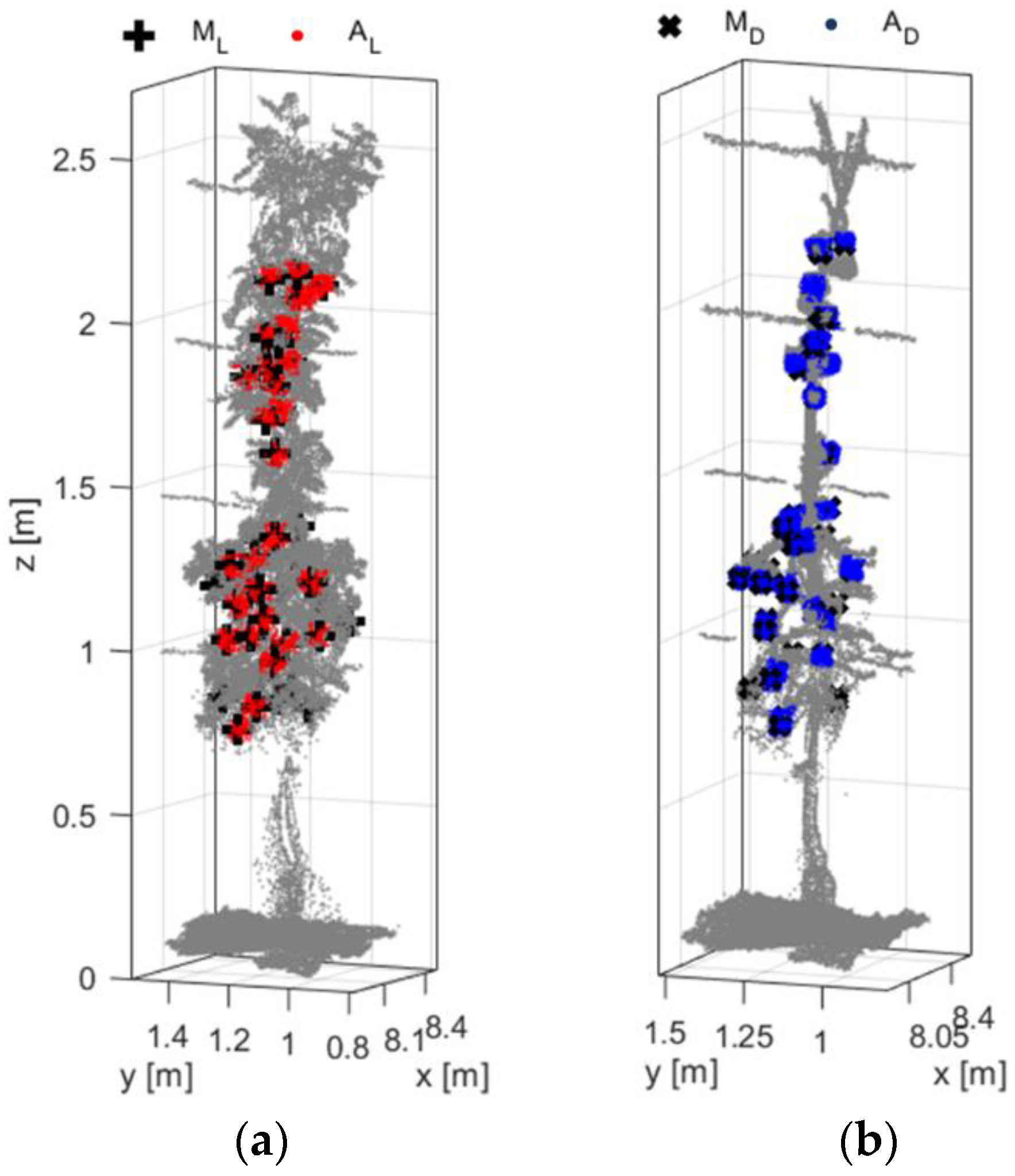
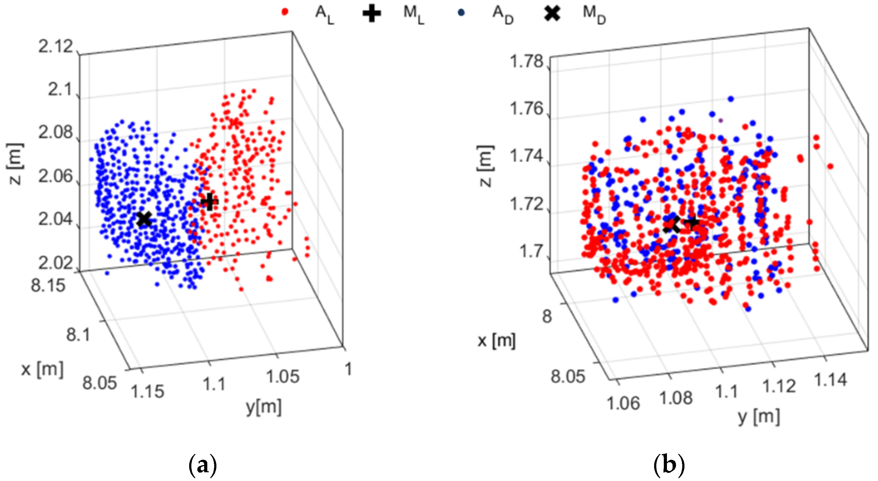
The differences of distance between the ML and MD (Figure 8) and the fruit diameter considering DD and DL were calculated for each measuring date (Table 3). The worst-case scenario was illustrated at DAFB42 with 19.9% RMSE (Figure 9a). Moreover, in the same growth stage, the highest difference between the DD and DL was revealed, presenting a mean difference of 22.3 mm with 0.3 mm SD. The measuring uncertainty was decreased at DAFB72. An even less pronounced RMSE was depicted at DAFB104, while the lowest difference between ground truth and estimated position of fruit center in foliated trees was found at DAFB120 (Table 3).
More specifically for DAFB120, the best-case scenario was depicted considering the position of apple center with a mean value of 0.1 mm difference and 5.7% RMSE (Figure 9b). Furthermore, the minimum difference between the DD and DL was analysed, reaching 8.7 mm with 0.1 mm SD and 9.5% RMSE.
4. Discussion
4.1. Segmentation
The application of a LiDAR sensor system enabled the acquisition of 3D point cloud of apple trees, allowing the utilization of radiometric (RToF) and geometric features (C, L) as classifiers for fruit detection in the proposed algorithm. The apple class (RA, CA, LA) was separated from leaves as well as delimited from the class capturing woody parts (RW, CW, LW). The latter thresholds were defined after tree defoliation, whereas, the leaf class for the same features (RL, CL, LL) was determined in TL. The discrete ranges (Figure 5) of RA (42–90%), RL (50 to 70%) and RW (0–60%) is assumed to be caused by their different type of surface [47] and water content [48]. Furthermore, the spherical shape of apples resulted in higher CA values (56–98%) than CW (0.1–55.2%) due to the linear shape of woody parts, while a reciprocal opposite range was observed in the correspondent classes of linearity, LA (0.2–38.3%) and LW (60.2–94.1%). Moreover, the latter classes were partly coinciding with CL (40–78%) and LL (20–80%). The apples were segmented from the woody parts and later clustered using the DBSCAN. The application of sphere in each MD enabled high resolution in the determination of Rth (76.1%), Cth (73.2%) and Lth (15.5%) at DAFB120. Similar value of Rth (60%) was suggested by Gene-Mola et al. [25] for the segmentation of apples in ‘Fuji’ trees.
This served as calibration for the segmentation modes, whereas also the sphere radius improved the detection of the number of fruit. As was previously mentioned, the ε of DBSCAN was based on the DManual of each ΔW at DAFB120. Thus, earlier growth stages would be influenced by the generation of augmented clusters. This was confirmed by the finding that the measuring uncertainty was elevated mainly in the DAFB42 stage, when a lower D of the fruits was measured manually.
Τhis overestimation of fruit size could result in under- and over-counting of the DBSCAN clustering at DAFB42 and subsequent measuring dates, respectively, since the ε remained constant, and the fruit may be bigger or more small fruits are collected in one cluster. In Sun et al. [34], the wide range of size and shape of cotton boll similarily influenced the splitting operation of clusters. Furthermore, the shape of apples is not perfectly spherical producing an error in the estimation of DD. Wang et al. [26] combined a cascade detection and an ellipse fitting to recognize and estimate the size of mangoes, using RGB-D depth imaging. However, the not perfectly elliptical shape of fruits produced 4.9 mm and 4.3 mm RMSE in the detected height and width of fruit, respectively. Gongal et al. [49] measured the size of apples based on the 3D coordinates from a 3D camera and they obtained 30.9% MAE, while the MAE decreased to 15.2% when the pixel information from an RGB camera was considered. As was mentioned before, the crop load (number of fruit per tree) varied, consequently trees with higher crop load will produce fuits of smaller size as found at DAFB120 compared to DAFB104. This affected the ratio of the total number of TP over the nD, decreasing it from 94.8% at DAFB120 (calibration date) to 88.4% at DAFB104.
Nevertheless, the present results indicate that the data set of L, C and RToF can enable feasible counting and sizing of apples from the 3D point cloud, allowing their discrimination even in areas with high apple density. Furthermore, the values of RToF, C and L were described through the surface of apples with sphere segmentation, increasing the resolution in the classes, and subsequently the determination of the mode value.
4.2. Evaluation
The apple clusters in TD were used as ground truth labels. This derived from the assumption that the shape and the size of apples could be fully described due to the reduced occlusions. Mack et al. [50] employed random sample consensus algorithm to fit a 3D sphere model in grapevine berries, reconstructing the shape of berries with 98% precision and 94% recall. However, the sphere size (DD) was also applied in TD as an additional step to evaluate the segmented region. In Rakun et al. [51], a reconstructed sphere to evaluate the 3D shape of segmented voxels was employed. Gene-Mola et al. [33] labelled manually the estimated locations of apples in the 3D point cloud, placing 3D rectangular bounding boxes on each apple. The reflectance and the sphericity derived from a LiDAR system were utilized as principal features in fruit detection, achieving 87.5% localization success and 0.85 F1. However, similar results have been reported from the implementation of 3D shape information with RGB vision systems, reaching a precision of 86.4% and recall 88.9% in fruit localization [35,36]. As a major perturbation factor, the woody parts in ΔW1-G revealed similar RToF and C values with the apples, enhancing the FP cases and subsequently the decline of accuracy in this region. The occlusions produced by branches and leaves hide partly or totally the fruit, resulting in undercounting of apples. Mendez et al. [52] used a LiDAR laser scanner to count the number of fruit in pruned orange trees (R2 = 0.63), however, similar to the results of the present study, the correlation was significantly reduced (R2 = 0.18) when the method was applied in unpruned trees due to occlusion by leaves.
The fruit size of the calibration data set reduced the accuracy of the method, when smaller fruit size occurred. The accuracy of the proposed methodology was reduced at the first two growth stages, resulting in the lowest percentage (65.8%) in ΔW4-3 at DAFB72. Stajnko et al. [53] monitored the diameter of green apples several times during the vegetation period, combining thermal and RGB camera. The highest relation between the manually measured and detected fruit diameter (R2 = 0.70) was observed at harvest stage, when the fruit reached their maximum size. Confirming, a less pronounced relation (R2 = 0.68) was observed in apples of smaller size after fruit drop. Furthermore, the varying fruit size, appearing even at one stage, can enhance the visual complexity of the cluster and consequently influence the identified number of fruit [54].
However, evaluating the distance of ML and MD centers allowed to quantify the possible deviations (Table 3). Some of the fruits were partly occluded by branches, creating smaller clusters in TL. This deviation was also visible in the high RMSE of fruit diameter considering DD and DL Summarizing, pomising results for in situ yield monitoring using a 2D LiDAR sensor system. Further research should be carried out to test the method in different apple cultivars having less spherical shape and varying surfaces properties in order to identify and tackle possible deviations of geometric and reflectance values.
5. Conclusions
The radiometric and geometric features of apples (RA, CA, LA) showed higher values compared to wood and leaves compared to fruit elements. Concluding that they can be utilized to segment the apple points in the 3D point cloud. The likelihood of thresholds was enhanced by integrating a sphere to segment the apple clusters and determine the center position. This calibration was carried out on two defoliated trees at DAFB120, resulting in Rth = 76.1%, Cth = 73.2%, and Lth = 15.5% that define the points of apple class.
The developed sphere methodology in defoliated trees was able to estimate the fruit diameter, DD, with low measuring uncertainty at different growth stages. The DD, showed the highest adjacent coefficient of determination (R2adj = 0.95) with DManual in the upper parts of the canopy (ΔW4-3) at DAFB104, when the fruit showed hardly any occlusion with other tree organs and fruit size was at maximum considering all trees measured.
The evaluation of apple clusters in foliated trees over the clusters of defoliated trees depicted that the robustness is affected by the fruit size, but resulted in highest performance of 89.5% F1 with 91.0% recall and 88.2% precision. At DAFB120, the minimum difference between ground truth, DD, and estimated, DL, fruit diameter was 8.7 mm representing 9.5% RMSE, which encourages the further development of LiDAR-based fruit size analysis.
Author Contributions
N.T. developed the experimental plan, carried out the data analysis, programmed the codes applied, and wrote the text. D.S.P. contributed to the programming and added directions on the data analysis. G.X. supported the experimental planning, data analysis, and revision of the text. M.Z.-S. developed the experimental plan, added directions to the data analysis and interpretation, and revised the text. All authors have read and agreed to the published version of the manuscript.
Funding
This research was funded by PRIMEFRUIT project in the framework of European Innovation Partnership (EIP) granted by Ministerium für Ländliche Entwicklung, Umwelt und Landwirtschaft (MLUL) Brandenburg, Investitionsbank des Landes Brandenburg, grant number 80168342.
Acknowledgments
The authors are grateful that the publication of this article was funded by the Open Access Fund of the Leibniz Association.
Conflicts of Interest
The authors declare no conflict of interest
Abbreviations
| AD | Points of apple class on defoliated trees |
| AL | Points of apple class on trees with leaves |
| C | Curvature estimated by eigenvalues [%] |
| Mean value of curvature in defoliated trees [%] | |
| CA | Curvature of apple class [%] |
| CL | Curvature of leaf class [%] |
| CW | Curvature of wood class [%] |
| Cth | Curvature threshold with the highest likelihood within the apple class [%] |
| Cov | Covariance matrix of the k-nearest neighbors points, Pi |
| DManual | Manually measured diameter of apples [mm] |
| DD | Estimated diameter of apple cluster or subcluster in defoliated trees [mm] |
| DL | Estimated diameter of apple cluster or subcluster in foliated trees [mm] |
| DAFB | Days after full bloom |
| FN | False negatives |
| FP | False positives |
| K | Total number of point set defined from k-nearest neighbors algorithm |
| L | Linearity estimated by eigenvalues [%] |
| LA | Linearity of apple class [%] |
| LL | Linearity of leaf class [%] |
| LW | Linearity of wood class [%] |
| Lth | Linearity threshold with the highest likelihood within apple class [%] |
| MD | Center of fruit points created by k-means clustering in defoliated trees |
| ML | Center of apple created by k-means clustering in foliated trees |
| MAE | Mean absolute error [mm] |
| MBE | Mean bias error [mm] |
| N | The sum of true positives, true negatives, false positives, false negatives |
| n | Total number of samples |
| nD | Total number of apple clusters in defoliated trees. |
| nManual | Total number of manually counted apples |
| Pi | Set of points defined from k-nearest neighbors algorithm |
| Average of set of points defined from k-nearest neighbors algorithm | |
| r | Radius used in the k-nearest neighbors [mm] |
| RToF | Apparent reflectance intensity at 905 nm of LiDAR laser scanner [%] |
| Mean value of apparent reflectance intensity in defoliated trees [%] | |
| RA | Apparent reflectance intensity of apple class [%] |
| RL | Apparent reflectance intensity of leaf class [%] |
| RW | Apparent reflectance intensity of wood class [%] |
| Rth | Apparent reflectance intensity threshold with the highest likelihood within the apple class [%] |
| RMSE | Root mean square error [%] |
| Rmin | Reflectance of board target coated with urethane [%] |
| Rmax | Reflectance of board target coated with barium sulphate [%] |
| ToF | Time of flight |
| TD | Trees after defoliation |
| TL | Trees before defoliation |
| TN | True negatives |
| TP | True positives |
| W1, W2, W3, W4 | Four horizontally parallel wires supporting the trees |
| ΔW | Tree region between the ground and W1, W2, W3, W4 |
| [] | Points in three dimensions |
| ε | Search radius used in density-based scan algorithm |
| Eigenvalues calculated from the covariance matrix |
References
- Zude-Sasse, M.; Fountas, S.; Gemtos, T.A.; Abu-Khalaf, N. Applications of precision agriculture in horticultural crops. Eur. J. Hortic. Sci. 2016, 81, 78–90. [Google Scholar] [CrossRef]
- Gemtos, T.; Fountas, S.; Tagarakis, A.; Liakos, V. Precision agriculture application in fruit crops: Experience in handpicked fruits. Procedia Technol. 2013. [Google Scholar] [CrossRef] [Green Version]
- Mosleh, M.K.; Hassan, Q.K.; Chowdhury, E.H. Application of remote sensors in mapping rice area and forecasting its production: A review. Sensors 2015, 15, 769–791. [Google Scholar] [CrossRef] [PubMed] [Green Version]
- Yang, C.; Anderson, G.L. Mapping grain sorghum yield variability using airborne digital videography. Precis. Agric. 2000, 2, 7–23. [Google Scholar] [CrossRef]
- Pantazi, X.E.; Moshou, D.; Alexandridis, T.; Whetton, R.L.; Mouazen, A.M. Wheat yield prediction using machine learning and advanced sensing techniques. Comput. Electron. Agric. 2016, 121, 57–65. [Google Scholar] [CrossRef]
- Schwalbert, R.A.; Amado, T.J.C.; Nieto, L.; Varela, S.; Corassa, G.M.; Horbe, T.A.N.; Rice, C.W.; Peralta, N.R.; Ciampitti, I.A. Forecasting maize yield at field scale based on high-resolution satellite imagery. Biosyst. Eng. 2018, 171, 179–192. [Google Scholar] [CrossRef]
- Tsoulias, N.; Paraforos, D.S.; Fountas, S.; Zude-Sasse, M. Calculating the water deficit spatially using LiDAR laser scanner in an apple orchard. In Precision Agriculture 2019—Papers, Proceedings of the 12th European Conference on Precision Agriculture, ECPA 2019, Montpellier, France, 8–11 July 2019; Wageningen Academic Publishers: Wageningen, The Netherlands, 2019. [Google Scholar]
- Gongal, A.; Amatya, S.; Karkee, M.; Zhang, Q.; Lewis, K. Sensors and systems for fruit detection and localization: A review. Comput. Electron. Agric. 2015, 116, 8–19. [Google Scholar] [CrossRef]
- Linker, R. A procedure for estimating the number of green mature apples in night-time orchard images using light distribution and its application to yield estimation. Precis. Agric. 2017, 18, 59–75. [Google Scholar] [CrossRef]
- Bargoti, S.; Underwood, J. Deep fruit detection in orchards. In Proceedings of the 2017 IEEE International Conference on Robotics and Automation (ICRA), Singapore, 29 May–3 June 2017; pp. 3626–3633. [Google Scholar] [CrossRef] [Green Version]
- Dorj, U.O.; Lee, M.; Yun, S.S. An yield estimation in citrus orchards via fruit detection and counting using image processing. Comput. Electron. Agric. 2017, 140, 103–112. [Google Scholar] [CrossRef]
- Sengupta, S.; Lee, W.S. Identification and determination of the number of immature green citrus fruit in a canopy under different ambient light conditions. Biosyst. Eng. 2014. [Google Scholar] [CrossRef]
- Qureshi, W.S.; Payne, A.; Walsh, K.B.; Linker, R.; Cohen, O.; Dailey, M.N. Machine vision for counting fruit on mango tree canopies. Precis. Agric. 2017, 18, 224–244. [Google Scholar] [CrossRef]
- Luo, L.; Tang, Y.; Zou, X.; Wang, C.; Zhang, P.; Feng, W. Robust Grape Cluster Detection in a Vineyard by Combining the AdaBoost Framework and Multiple Color Components. Sensors 2016, 16, 2098. [Google Scholar] [CrossRef] [PubMed]
- Linker, R.; Cohen, O.; Naor, A. Determination of the number of green apples in RGB images recorded in orchards. Comput. Electron. Agric. 2012, 81, 45–57. [Google Scholar] [CrossRef]
- Kurtulmus, F.; Lee, W.S.; Vardar, A. Immature peach detection in colour images acquired in natural illumination conditions using statistical classifiers and neural network. Precis. Agric. 2014. [Google Scholar] [CrossRef]
- Wachs, J.P.; Stern, H.I.; Burks, T.; Alchanatis, V. Low and high-level visual feature-based apple detection from multi-modal images. Precis. Agric. 2010. [Google Scholar] [CrossRef]
- Gan, H.; Lee, W.S.; Alchanatis, V.; Ehsani, R.; Schueller, J.K. Immature green citrus fruit detection using color and thermal images. Comput. Electron. Agric. 2018, 152, 117–125. [Google Scholar] [CrossRef]
- Zude, M. Comparison of indices and multivariate models to non-destructively predict the fruit chlorophyll by means of visible spectrometry in apple fruit. Anal. Chim. Acta 2003. [Google Scholar] [CrossRef]
- Sa, I.; Ge, Z.; Dayoub, F.; Upcroft, B.; Perez, T.; McCool, C. Deepfruits: A fruit detection system using deep neural networks. Sensors 2016, 16, 1222. [Google Scholar] [CrossRef] [Green Version]
- Feng, J.; Zeng, L.; He, L. Apple fruit recognition algorithm based on multi-spectral dynamic image analysis. Sensors 2019, 19, 949. [Google Scholar] [CrossRef] [Green Version]
- Taylor, J.A.; Dresser, J.L.; Hickey, C.C.; Nuske, S.T.; Bates, T.R. Considerations on spatial crop load mapping. Aust. J. Grape Wine Res. 2019, 25, 144–155. [Google Scholar] [CrossRef]
- Gutiérrez, S.; Wendel, A.; Underwood, J. Ground based hyperspectral imaging for extensive mango yield estimation. Comput. Electron. Agric. 2019, 157, 126–135. [Google Scholar] [CrossRef]
- Vázquez-Arellano, M.; Griepentrog, H.W.; Reiser, D.; Paraforos, D.S. 3-D imaging systems for agricultural applications—A review. Sensors 2016, 16, 618. [Google Scholar] [CrossRef] [PubMed] [Green Version]
- Gené-Mola, J.; Vilaplana, V.; Rosell-Polo, J.R.; Morros, J.R.; Ruiz-Hidalgo, J.; Gregorio, E. Multi-modal deep learning for Fuji apple detection using RGB-D cameras and their radiometric capabilities. Comput. Electron. Agric. 2019, 162, 689–698. [Google Scholar] [CrossRef]
- Wang, Z.; Walsh, K.B.; Verma, B. On-tree mango fruit size estimation using RGB-D images. Sensors 2017, 17, 2738. [Google Scholar] [CrossRef] [PubMed] [Green Version]
- Kashani, A.G.; Olsen, M.J.; Parrish, C.E.; Wilson, N. A review of LIDAR radiometric processing: From ad hoc intensity correction to rigorous radiometric calibration. Sensors 2015, 15, 28099–28128. [Google Scholar] [CrossRef] [Green Version]
- Barnea, E.; Mairon, R.; Ben-Shahar, O. Colour-agnostic shape-based 3D fruit detection for crop harvesting robots. Biosyst. Eng. 2016, 146, 57–70. [Google Scholar] [CrossRef]
- Brodu, N.; Lague, D. 3D terrestrial lidar data classification of complex natural scenes using a multi-scale dimensionality criterion: Applications in geomorphology. ISPRS J. Photogramm. Remote Sens. 2012, 68, 121–134. [Google Scholar] [CrossRef] [Green Version]
- Zhu, X.; Skidmore, A.K.; Darvishzadeh, R.; Niemann, K.O.; Liu, J.; Shi, Y.; Wang, T. Foliar and woody materials discriminated using terrestrial LiDAR in a mixed natural forest. Int. J. Appl. Earth Obs. Geoinf. 2018, 64, 43–50. [Google Scholar] [CrossRef]
- Ma, L.; Zheng, G.; Eitel, J.U.H.; Moskal, L.M.; He, W.; Huang, H. Improved salient feature-based approach for automatically separating photosynthetic and nonphotosynthetic components within terrestrial Lidar point cloud data of forest canopies. IEEE Trans. Geosci. Remote Sens. 2016. [Google Scholar] [CrossRef]
- Kuo, K.; Itakura, K.; Hosoi, F. Leaf segmentation based on k-means algorithm to obtain leaf angle distribution using terrestrial LiDAR. Remote Sens. 2019, 11, 2536. [Google Scholar] [CrossRef] [Green Version]
- Gené-Mola, J.; Gregorio, E.; Guevara, J.; Auat, F.; Sanz-Cortiella, R.; Escolà, A.; Llorens, J.; Morros, J.R.; Ruiz-Hidalgo, J.; Vilaplana, V.; et al. Fruit detection in an apple orchard using a mobile terrestrial laser scanner. Biosyst. Eng. 2019, 187, 171–184. [Google Scholar] [CrossRef]
- Sun, S.; Li, C.; Chee, P.W.; Paterson, A.H.; Jiang, Y.; Xu, R.; Robertson, J.S.; Adhikari, J.; Shehzad, T. Three-dimensional photogrammetric mapping of cotton bolls in situ based on point cloud segmentation and clustering. ISPRS J. Photogramm. Remote Sens. 2020, 160, 195–207. [Google Scholar] [CrossRef]
- Tao, Y.; Zhou, J. Automatic apple recognition based on the fusion of color and 3D feature for robotic fruit picking. Comput. Electron. Agric. 2017, 142, 388–396. [Google Scholar] [CrossRef]
- Lin, G.; Tang, Y.; Zou, X.; Xiong, J.; Fang, Y. Color-, depth-, and shape-based 3D fruit detection. Precis. Agric. 2020, 21, 1–17. [Google Scholar] [CrossRef]
- Tsoulias, N.; Paraforos, D.S.; Fountas, S.; Zude-Sasse, M. Estimating canopy parameters based on the stem position in apple trees using a 2D lidar. Agronomy 2019, 9, 740. [Google Scholar] [CrossRef] [Green Version]
- Soudarissanane, S.; Lindenbergh, R.; Menenti, M.; Teunissen, P. Scanning geometry: Influencing factor on the quality of terrestrial laser scanning points. ISPRS J. Photogramm. Remote Sens. 2011, 66, 389–399. [Google Scholar] [CrossRef]
- Kaasalainen, S.; Krooks, A.; Kukko, A.; Kaartinen, H. Radiometric calibration of terrestrial laser scanners withexternal reference targets. Remote Sens. 2009, 1, 144–158. [Google Scholar] [CrossRef] [Green Version]
- Kooi, B. MTi User Manual; MTi 10-Series and MTi 100-Series; Doc. MT0605P.B; Xsens Technologies: Enschede, The Netherlands, 2016; pp. 35–36. [Google Scholar]
- Vázquez-Arellano, M.; Reiser, D.; Paraforos, D.S.; Garrido-Izard, M.; Burce, M.E.C.; Griepentrog, H.W. 3-D reconstruction of maize plants using a time-of-flight camera. Comput. Electron. Agric. 2018, 145, 235–247. [Google Scholar] [CrossRef]
- Sadar, N.; Urbanek-Krajnc, A.; Unuk, T. Spectrophotometrically determined pigment contents of intact apple fruits and their relations with quality: A review. Zemdirbyste 2013. [Google Scholar] [CrossRef] [Green Version]
- Hackel, T.; Wegner, J.D.; Schindler, K. Contour detection in unstructured 3D point clouds. In Proceedings of the IEEE Conference on Computer Vision and Pattern Recognition, Las Vegas, NV, USA, 27–30 June 2016; pp. 1610–1618. [Google Scholar] [CrossRef]
- Lin, C.H.; Chen, J.Y.; Su, P.L.; Chen, C.H. Eigen-feature analysis of weighted covariance matrices for LiDAR point cloud classification. ISPRS J. Photogramm. Remote Sens. 2014, 94, 70–79. [Google Scholar] [CrossRef]
- Koenig, K.; Höfle, B.; Hämmerle, M.; Jarmer, T.; Siegmann, B.; Lilienthal, H. Comparative classification analysis of post-harvest growth detection from terrestrial LiDAR point clouds in precision agriculture. ISPRS J. Photogramm. Remote Sens. 2015. [Google Scholar] [CrossRef]
- Ester, M.; Kriegel, H.-P.; Sander, J.; Xu, X. A Density-Based Algorithm for Discovering Clusters in Large Spatial Databases with Noise. In Proceedings of the 2nd International Conference on Knowledge Discovery and Data Mining, Oregon, Portland, 2–4 August 1996. [Google Scholar]
- Kaasalainen, S.; Jaakkola, A.; Kaasalainen, M.; Krooks, A.; Kukko, A. Analysis of incidence angle and distance effects on terrestrial laser scanner intensity: Search for correction methods. Remote Sens. 2011, 3, 2207–2221. [Google Scholar] [CrossRef] [Green Version]
- Zhu, X.; Wang, T.; Skidmore, A.K.; Darvishzadeh, R.; Niemann, K.O.; Liu, J. Canopy leaf water content estimated using terrestrial LiDAR. Agric. For. Meteorol. 2017. [Google Scholar] [CrossRef]
- Gongal, A.; Karkee, M.; Amatya, S. Apple fruit size estimation using a 3D machine vision system. Inf. Process. Agric. 2018, 5, 498–503. [Google Scholar] [CrossRef]
- Mack, J.; Lenz, C.; Teutrine, J.; Steinhage, V. High-precision 3D detection and reconstruction of grapes from laser range data for efficient phenotyping based on supervised learning. Comput. Electron. Agric. 2017. [Google Scholar] [CrossRef]
- Rakun, J.; Stajnko, D.; Zazula, D. Detecting fruits in natural scenes by using spatial-frequency based texture analysis and multiview geometry. Comput. Electron. Agric. 2011, 76, 80–88. [Google Scholar] [CrossRef]
- Méndez, V.; Pérez-Romero, A.; Sola-Guirado, R.; Miranda-Fuentes, A.; Manzano-Agugliaro, F.; Zapata-Sierra, A.; Rodríguez-Lizana, A. In-field estimation of orange number and size by 3D laser scanning. Agronomy 2019, 9, 885. [Google Scholar] [CrossRef] [Green Version]
- Stajnko, D.; Lakota, M.; Hočevar, M. Estimation of number and diameter of apple fruits in an orchard during the growing season by thermal imaging. Comput. Electron. Agric. 2004. [Google Scholar] [CrossRef]
- Kurtulmus, F.; Lee, W.S.; Vardar, A. Green citrus detection using “eigenfruit”, color and circular Gabor texture features under natural outdoor conditions. Comput. Electron. Agric. 2011. [Google Scholar] [CrossRef]
Figure 1.
Flowchart showing the protocol for apple detection and sizing using defoliated trees (TD), starting with the threshold application in the registered point cloud pair, through the filtering and partitioning, until the counting of clusters, which were compared to reference data from manual measurements and applied as ground truth when analysing the foliated trees. The cells with shading and dashed frame point out the differences from apple detection in foliated trees.

Figure 2.
Flowchart of the validation showing the protocol for apple detection and sizing using foliated (TL) trees, starting with the threshold application in the registered point cloud, through the filtering and partitioning, until the counting of centers of clusters. The cell with shading and dashed frame point out the inclusion of leaf class in the analysis.

Figure 3.
Representation of 3D point clouds of (a) RGB image (b) reflectance (RToF) [%], (c) curvature (C) [%] and (d) linearity (L) [%] of trees measured with leaves at DAFB120.
Figure 3.
Representation of 3D point clouds of (a) RGB image (b) reflectance (RToF) [%], (c) curvature (C) [%] and (d) linearity (L) [%] of trees measured with leaves at DAFB120.

Figure 4.
Representation of 3D point clouds of (a) RGB image (b) reflectance (RToF) [%], (c) curvature (C) [%] and (d) linearity (L) [%] in defoliated trees at DAFB120.
Figure 4.
Representation of 3D point clouds of (a) RGB image (b) reflectance (RToF) [%], (c) curvature (C) [%] and (d) linearity (L) [%] in defoliated trees at DAFB120.

Figure 5.
The probability density of (a) calibrated reflectance intensity (RToF) [%], (b) curvature (C) [%], and (c) linearity (L) [%] for wood, leaves, and apples.
Figure 5.
The probability density of (a) calibrated reflectance intensity (RToF) [%], (b) curvature (C) [%], and (c) linearity (L) [%] for wood, leaves, and apples.

Figure 6.
Box-Whisker plot of segmented points of wood (W), leaves (L) and apples (A) based on reflectance (RToF), curvature (C) and linearity (L) showing the mean and mode values, maximum, minimum, standard deviation are represented by lower and upper edges of the box, the dash in each box indicates the median.

Figure 7.
Detection of apple centers (MD) using sphere segmentation (b) enlargement of upper zone of the tree with points of apples class enveloped in the sphere. The blue color depicts the apple points of the defoliated trees (AD).
Figure 7.
Detection of apple centers (MD) using sphere segmentation (b) enlargement of upper zone of the tree with points of apples class enveloped in the sphere. The blue color depicts the apple points of the defoliated trees (AD).

Figure 8.
Representation of (a) detected centers in foliated trees (ML) and (b) after defoliation (MD). The red color depicts the apple points of the foliated tree (AL) while the blue color show the points of the fruits in the defoliated tree (AD).
Figure 8.
Representation of (a) detected centers in foliated trees (ML) and (b) after defoliation (MD). The red color depicts the apple points of the foliated tree (AL) while the blue color show the points of the fruits in the defoliated tree (AD).

Figure 9.
Representation of the (a) worst- and the (b) best-case scenario of the distance of the center of clusters in defoliated (MD) and foliated (ML) trees at DAFB42 and DAFB120. The red color depicts the apple points of the foliated trees (AL) while the blue color the points of the defoliated tree (AD).


Table 1.
Results of manually measured mean diameter (DManual) [mm] and the mean LiDAR-based measurement (DD) [mm] in defoliated trees regarding mean absolute error (MAE) [mm], bias (MBE) [mm], root mean square error (RMSE) [%], and adjusted coefficient of determination (R2adj).
Table 1.
Results of manually measured mean diameter (DManual) [mm] and the mean LiDAR-based measurement (DD) [mm] in defoliated trees regarding mean absolute error (MAE) [mm], bias (MBE) [mm], root mean square error (RMSE) [%], and adjusted coefficient of determination (R2adj).
| DManual [mm] | DD [mm] | MBE [mm] | MAE [mm] | RMSE [%] | R2adj | ||
|---|---|---|---|---|---|---|---|
| DAFB42 | ΔW1-G | 32.0 | 47.6 | 6.5 | 7.4 | 10.8 | 0.46 |
| ΔW2-1 | 36.1 | 65.1 | 7.5 | 8.7 | 12.0 | 0.45 | |
| ΔW3-2 | 39.2 | 47.9 | 4.7 | 5.5 | 7.2 | 0.69 | |
| ΔW4-3 | 39.3 | 41.2 | 5.3 | 6.2 | 6.6 | 0.74 | |
| DAFB72 | ΔW1-G | 66.4 | 48.0 | −10.7 | 12.4 | 14.5 | 0.42 |
| ΔW2-1 | 62.8 | 37.9 | −9.11 | 10.5 | 15.8 | 0.38 | |
| ΔW3-2 | 65.6 | 63.7 | −3.2 | 4.6 | 5.7 | 0.81 | |
| ΔW4-3 | 67.0 | 63.7 | −3.8 | 4.4 | 5.9 | 0.82 | |
| DAFB104 | ΔW1-G | 74.8 | 70.3 | −5.8 | 8.3 | 9.6 | 0.55 |
| ΔW2-1 | 71.1 | 69.5 | −4.5 | 5.1 | 7.8 | 0.66 | |
| ΔW3-2 | 69.6 | 68.7 | −3.3 | 3.8 | 4.5 | 0.90 | |
| ΔW4-3 | 74.8 | 70.3 | −3.2 | 3.5 | 4.1 | 0.95 | |
| DAFB120 | ΔW1-G | 69.3 | 67.3 | −6.1 | 7.1 | 7.7 | 0.67 |
| ΔW2-1 | 70.5 | 68.4 | −5.6 | 6.5 | 6.8 | 0.74 | |
| ΔW3-2 | 69.7 | 68.6 | −4.3 | 4.9 | 5.8 | 0.81 | |
| ΔW4-3 | 68.6 | 66.4 | −5.3 | 6.1 | 6.6 | 0.75 |
Table 2.
Performance assessment of the localization algorithm on the segmented apple points in foliated trees (TL) considering the apple in defoliated trees (TD) as ground truth over four growth stages given in days after full bloom (DAFB) and in four tree height (W) starting from ground (G) till the maximum tree point (4). Manually counted fruit number (nManual), total number of detected fruits in TD (nD) and true positives (TP) in TL with descriptive statistics are given.
| nManual | nD | TP | Accuracy [%] | Precision [%] | Recall [%] | F1 [%] | ||
|---|---|---|---|---|---|---|---|---|
| DAFB42 | ΔW1-G | 10 | 10 | 9 | 76.9 | 80.0 | 83.8 | 81.8 |
| ΔW2-1 | 19 | 18 | 16 | 85.2 | 82.6 | 86.3 | 84.4 | |
| ΔW3-2 | 34 | 34 | 30 | 74.5 | 75.6 | 83.7 | 79.4 | |
| ΔW4-3 | 17 | 17 | 15 | 76.9 | 85.0 | 89.4 | 87.1 | |
| DAFB72, | ΔW1-G | 6 | 6 | 6 | 71.4 | 85.7 | 80.8 | 83.1 |
| ΔW2-1 | 15 | 14 | 12 | 75.1 | 82.8 | 82.3 | 82.5 | |
| ΔW3-2 | 14 | 14 | 12 | 73.3 | 83.3 | 86.6 | 84.9 | |
| ΔW4-3 | 7 | 7 | 5 | 65.8 | 71.4 | 83.3 | 76.9 | |
| DAFB104, | ΔW1-G | 11 | 11 | 9 | 77.2 | 81.1 | 88.8 | 84.7 |
| ΔW2-1 | 18 | 18 | 16 | 84.1 | 85.7 | 81.8 | 83.3 | |
| ΔW3-2 | 11 | 11 | 10 | 82.5 | 85.7 | 87.0 | 86.3 | |
| ΔW4-3 | 12 | 12 | 11 | 80.2 | 86.6 | 88.5 | 87.5 | |
| DAFB120 | ΔW1-G | 15 | 15 | 14 | 73.4 | 78.9 | 83.3 | 81.1 |
| ΔW2-1 | 32 | 31 | 28 | 76.4 | 82.2 | 84.2 | 83.1 | |
| ΔW3-2 | 16 | 16 | 16 | 75.5 | 85.7 | 88.0 | 86.8 | |
| ΔW4-3 | 15 | 15 | 15 | 88.9 | 88.2 | 91.0 | 89.5 |
Table 3.
Differences between the position of the centers of defoliated (MD) and foliated (ML) clusters as well as the fruit diameter estimated (DL) and ground truth (DD) in TL and in TD, respectively, regarding the standard deviation (SD) and root mean square error (RMSE) [%] during the fruit growth given in days after full bloom (DAFB).
| MD–ML [mm] | SD [mm] | RMSE [%] | DD–DL [mm] | SD [mm] | RMSE [%] | |
|---|---|---|---|---|---|---|
| DAFB42 | 0.2 | 0.22 | 19.9 | 22.3 | 0.3 | 16.3 |
| DAFB72 | 0.1 | 0.1 | 15.1 | 12.6 | 0.2 | 13.7 |
| DAFB104 | 0.1 | 0.1 | 6.7 | 11.3 | 0.2 | 10.3 |
| DAFB120 | 0.1 | 0.1 | 5.7 | 8.7 | 0.1 | 9.5 |
© 2020 by the authors. Licensee MDPI, Basel, Switzerland. This article is an open access article distributed under the terms and conditions of the Creative Commons Attribution (CC BY) license (http://creativecommons.org/licenses/by/4.0/).
Share and Cite
MDPI and ACS Style
Tsoulias, N.; Paraforos, D.S.; Xanthopoulos, G.; Zude-Sasse, M. Apple Shape Detection Based on Geometric and Radiometric Features Using a LiDAR Laser Scanner. Remote Sens. 2020, 12, 2481. https://doi.org/10.3390/rs12152481
AMA Style
Tsoulias N, Paraforos DS, Xanthopoulos G, Zude-Sasse M. Apple Shape Detection Based on Geometric and Radiometric Features Using a LiDAR Laser Scanner. Remote Sensing. 2020; 12(15):2481. https://doi.org/10.3390/rs12152481
Chicago/Turabian StyleTsoulias, Nikos, Dimitrios S. Paraforos, George Xanthopoulos, and Manuela Zude-Sasse. 2020. "Apple Shape Detection Based on Geometric and Radiometric Features Using a LiDAR Laser Scanner" Remote Sensing 12, no. 15: 2481. https://doi.org/10.3390/rs12152481
Note that from the first issue of 2016, this journal uses article numbers instead of page numbers. See further details here.