Article

Sensitivity of Earthquake Damage Estimation to the Input Data (Soil Characterization Maps and Building Exposure): Case Study in the Luchon Valley, France

1
Department of Risks and Prevention, French Geological Survey BRGM, 45060 Orléans, France
2
European Centre for Training and Research in Earthquake Engineering (EUCENTRE), 27100 Pavia, Italy
*
Author to whom correspondence should be addressed.
Geosciences 2021, 11(6), 249; https://doi.org/10.3390/geosciences11060249
Submission received: 4 May 2021 / Revised: 28 May 2021 / Accepted: 1 June 2021 / Published: 7 June 2021

Abstract

:
This article studies the effects of the soil data and exposure data of residential building inventories, as well as their spatial resolution, on seismic damage and loss estimates for a given earthquake scenario. Our aim is to investigate how beneficial it would be to acquire higher resolution inventories at the cost of additional effort and resources. Seismic damage computations are used to evaluate the relative influence of varying spatial resolution on a given damage model, where other parameters were held constant. We use soil characterization maps and building exposure inventories, provided at different scales from different sources: the European database, a national dataset at the municipality scale, and local field investigations. Soil characteristics are used to evaluate site effects and to assign amplification factors to the strong motion applied to the exposed areas. Exposure datasets are used to assign vulnerability indices to sets of buildings, from which a damage distribution is produced (based on the applied seismic intensity). The different spatial resolutions are benchmarked in a case-study area which is subject to moderate-to-average seismicity levels (Luchon valley in the Pyrénées, France). It was found that the proportion of heavily damaged buildings is underestimated when using the European soil map and the European building database, while the more refined databases (national/regional vs. local maps) result in similar estimates for moderate earthquake scenarios. Finally, we highlight the importance of pooling open access data from different sources, but caution the challenges of combining different datasets, especially depending on the type of application that is pursued (e.g., for risk mitigation or rapid response tools).

1. Introduction

Earthquake risk assessment is a complex exercise, involving the assimilation of geological, seismological, engineering, demographic, and economic data within a risk assessment model [1]. Significant efforts have been made in the last 25 years towards the development of regional, national, continental, or even global seismic hazard and risk models, such as the National Risk Assessment (NRA) for Italy [2], the Global Earthquake Risk Model developed by the Global Earthquake Model (GEM) Foundation [3] and, more recently, the European Seismic Risk Model ERSSRM20, which is an output of the European Horizon 2020 SERA project [4], building upon the research efforts of many previous projects (e.g., LESSLOSS, SYNER-G, and NERA-SHARE) [5]. Seismic loss scenarios are core elements for the planning and management of seismic emergencies at the national and regional scale, in order to evaluate how much loss a region might experience from a given earthquake [6]. A loss study may include estimates of deaths and injuries; property losses; loss of function in industries, lifelines, and emergency facilities; and economic impacts.
Emergency management in the immediate post-earthquake period (e.g., search and rescue and emergency medical deployments) must allocate and prioritize resources to minimize the loss of life. When properly coordinated, emergency response capabilities can be significantly improved, in order to reduce casualties and facilitate evacuation by permitting the rapid and effective deployment of emergency operations. To this end, there exist many near-real-time loss estimation tools, which are capable of computing damage and casualties in near-real-time for several regions of the world [7,8], where rapid estimates of ground-shaking are usually coupled with building exposure inventories and vulnerability relationships.
Seismic damage assessment requires taking three main factors into consideration: hazard, exposure, and vulnerability. Hazard refers to a specific given scenario (deterministic study) or to the aggregation of all possible future occurrences of seismic events (probabilistic study) which may have adverse effects on vulnerable and exposed elements. On the other hand, exposure refers to the inventory of elements in an area in which the hazard may occur, while vulnerability refers to the susceptibility of exposed elements, such as physical components (e.g., buildings), human beings, and their livelihoods, to suffer adverse effects when subjected to the hazard. Several models have been developed for assessing the vulnerability of buildings and estimating the expected earthquake damages and losses for a given scenario. The methods developed may be empirical, analytical, or mechanical, based on fragility curves of buildings or hybrid methods [9]. The methodological and input data choices inevitably introduce uncertainty in the results of the seismic risk assessment. A variety of uncertainties, originating from different sources, are present at every step of the risk assessment process (e.g., natural variability of the phenomena under investigation, incompleteness of input data, or inadequacies in the models and methods). Another essential source of uncertainty is related to the spatial resolution of exposure units [10].
Corbane et al. [1] shed light on the influence of methodological and data input choices on the risk estimates at a pan-European level. Reliable inventories of the building stocks and soil characteristics, along with their spatial resolution, are crucial components in a given earthquake scenario, when the magnitude, epicenter, and fault mechanism are known. Besides this, the choice of an inventory and its spatial resolution depends not only on data availability and accessibility, as well as their degree of complexity and usability, but also on the purpose of the seismic risk assessment; for example, financial planning of earthquake losses, disaster risk mitigation, retrofit design, emergency rescue, and so on [11,12,13,14]. Bal et al. [15] showed that, for emergency response applications where the interest is in the distribution of damage as well as the total impact, a more refined spatial resolution of the exposure data is clearly a necessity.
The collection of harmonized data at a regional scale, as well as at the local scale, still represents one of the major challenges in seismic risk assessment studies. Preparing for data inventory is usually the most time-consuming and costly aspect of a loss study. It is also the most frustrating as, in principle, it is ideal to develop a perfect inventory; however, in practice, compromises must be made. It is wise to compile and update inventories that are as accurate as possible, under the circumstances and resources available.
In this study, we focus on two key inventories that are needed to estimate seismic damage: the soil database, which is part of the hazard factor when considering site amplification, and the building database, which establishes the exposure and vulnerability factors. The first inventory is about the local site conditions that have a great effect on earthquake losses. Due to local site effects, greater seismic losses often occur due to ground failures, increased intensity of shaking under some soil and topographic conditions, and selective amplification of ground motion at the frequencies critical to the structural response. While geotechnical data collected at individual construction sites can be very valuable in this effort, geological maps of districts and zones in a region—which are more commonly available—are more useful (e.g., [16,17]). Silva et al. [3] proposed that the relationship between a model’s resolution and the ground motion spatial correlation, as well as the consideration of local effects, such as ground motion site amplification, should be investigated further.
The second inventory is related to the buildings and their vulnerability. It provides the spatial distribution of buildings at the territorial scale (i.e., the number of buildings in each territorial unit of analysis), as well as the vulnerability classification of these buildings; that is, the seismic resistance considered by the adopted vulnerability model [18]. Census data on housing, which contain information on construction age, building material, and number of stories, are the primary source for building inventory, together with those on population, providing information about the exposure of the population through building occupancy. Building-by-building surveys, providing detailed data for single buildings in an investigated area, are the most complete source towards vulnerability classification. On the other hand, regional or national seismic damage assessments generally use information from remote sensing and national housing databases, where information is typically provided at a coarse resolution (i.e., at district or municipality level). In addition, exposure models of portfolios of buildings from the (re)insurance industry can be developed at a high resolution, as the location of each asset is documented. In these cases, spatial aggregation of the assets is performed, in order to minimize the computational effort. In all cases, Bal et al. [15] explained that, when the building stock data are aggregated, the modeler would usually assume each building class to be uniformly distributed over the area of the aggregated scale. In this case, the simplest approach would be to estimate the ground motions at a single point within each aggregated unit (e.g., administrative zone) and to use this value for all the damage calculations within that unit (which effectively models all the exposure data as being concentrated at this single point) [19,20]. The practical implementation of aggregated exposure models unavoidably includes some form of spatial aggregation. Furthermore, the aggregation and relocation of buildings result in a misrepresentation of the distance between the assets and the seismic sources [21]. Thus, such building exposure models add uncertainty to the damage assessment. Another important source of uncertainty arises from the grouping of the building inventory into a certain number of building classes, which depends on the detail of exposure information [22].
A question thus arises: to what extent is acquiring a higher resolution inventory beneficial? This article aims to study the effects of spatial scale (i.e., the resolution of input data describing the soil conditions and the characteristics of residential buildings) on the estimation of damage and loss for a given earthquake scenario, by considering either “weak data” (collected at a large-scale) or “more accurate”, yet more difficult-to-obtain, detailed surveys. Specifically, we address the question of how detailed such datasets should be, in order to yield a robust enough estimation of damage and loss, and how this affects the information delivered to operational emergency managers. We conduct this investigation in the Luchon valley, located in the French Pyrenees (Figure 1), due to the wealth of available data on the exposure of residential buildings and on local site effects at different scales (see Section 2). Descriptions of the different soil and building exposure inventories are presented in Section 3 and Section 4, respectively, as well as the approaches used to associate the soil amplification factors and the building vulnerability index. The structural damage is estimated using the intensity-based empirical vulnerability relationships developed by [23], without considering site effects at the first stage (constant PGA), to study the effect of exposure data resolution in a deterministic scenario; and with site amplifications at a second stage to study the effects of both soil and exposure data resolution on the damage estimates. Finally, two historical deterministic scenarios are studied. The findings of this study are detailed in Section 5 and Section 6. The objective of studying the two historical regional earthquakes is not to compare the damage prediction with the observed damages, but rather to illustrate the differences obtained using different resolutions of the input data. Indeed, for these two earthquakes, documentary archives do provide descriptions of the damage observed following these two earthquakes, but these observations cannot be used for validation, because the distribution and vulnerability of the buildings in 1855 and 1923 are very different from today.

2. Scenarios and Methodology

The risk evaluation procedure used herein consists of various steps, which are briefly outlined in this section. The first step of the procedure is to set the level of strong motion for rock conditions (i.e., without site effects), expressed in Peak Ground Acceleration (PGA), using either (i) a user-defined PGA map, or (ii) calculation performed using a ground motion prediction equation (GMPE), based on the magnitude and location of the scenario-earthquake assuming rock site conditions. Then, the impact of site effects on the PGA due to local variations in the near-surface lithology—and, possibly, topography (not considered here)—are modeled, by applying soil amplification coefficients using a site classification map (ideally coming from a seismic microzonation study). The PGA maps are then converted into macroseismic intensity, in terms of the EMS98 European Macroseismic Scale [25], using a ground-motion-to-intensity conversion equation (GMICE developed by [26]). The elements at risk (in this study, residential buildings) are characterized by vulnerability indices (Vi): a Vi value is assigned to each building type, defined in terms of its age, material, technique of construction and, potentially, other characteristics. Next, the damage degree is estimated, using the intensity-based empirical vulnerability relationships developed by [23] on the basis of the EMS98 macroseismic scale, where an analytical expression for the mean damage grade, μD (mean of the discrete beta distribution), is provided as a function of the macroseismic intensity and the Vi of a given building type. Finally, the distribution of damage at each location is assessed, based on μD and a value, t, which governs the spread of the discrete beta distribution. The outcome is the distribution, in terms of the six damage levels defined in the EMS98—D0 (undamaged), D1 (slight damage), D2 (moderate damage), D3 (heavy damage), D4 (partial collapse), and D5 (total collapse)—for each location, which are all separately considered. This procedure was implemented in the in-house BRGM software Armagedom, which was used for the computations presented here. Details on the procedure and the software are provided by [27,28,29].
We identified three sources for the databases, concerning the soil classification maps:
-
The European map (issued from SERA project), Municipal level [30];
-
The National map (issued from collaboration between BRGM and CCR), Municipal level [31]; and
-
The maps issued from microzonation studies at the specific area (SISPyr project), District level [32].
We also identified three databases for collecting data concerning building exposure:
-
The European database (issued from SERA project), Municipal level [33];
-
Data from the French national statistics institute (INSEE), Municipal level—in which the spatial distribution is juxtaposed with the occupancy areas [34]; and
-
Data issued from site inspection at the specific area (SISPyr project), district level [35].
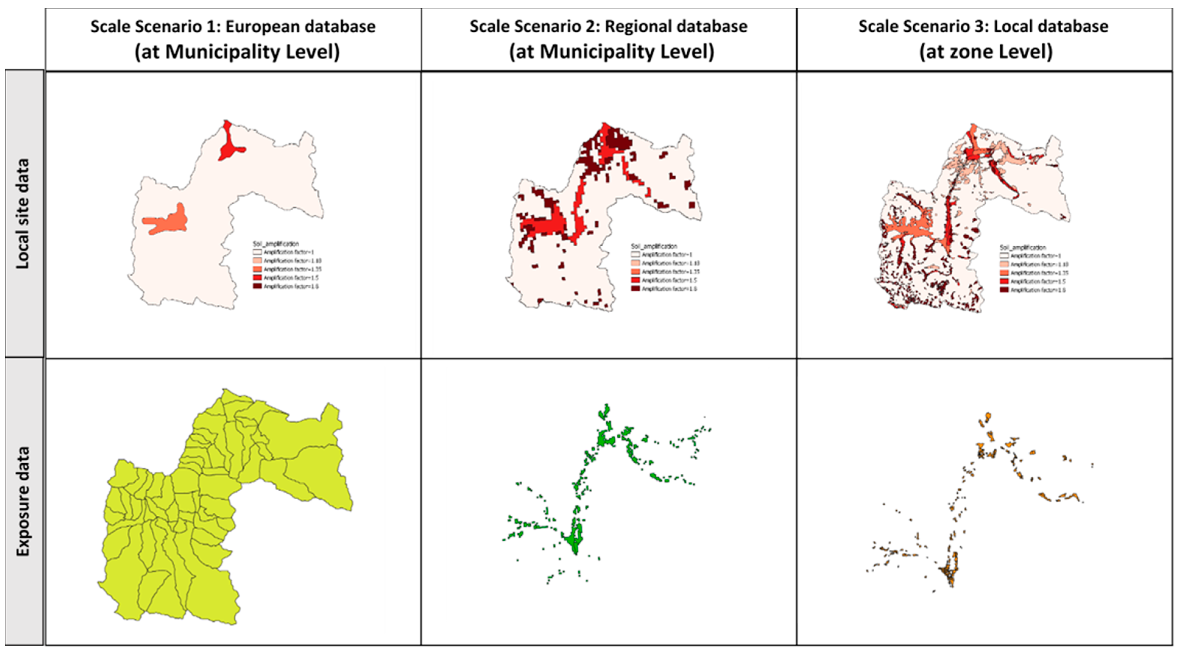
Therefore, we defined three scale scenarios, in order to estimate the seismic damage corresponding to a given ground-motion scenario, using the various data sources:
SS1—Europe: using the European soil map and the European database for the buildings, at the municipal level;
SS2—France: using the National soil map and the national statistics database for the buildings, at the municipal level; and
SS3—Luchon: using the soil maps and building data issued at the district level.
In the following, we collect and harmonize the input data for the three scale scenarios (SS), corresponding to different scales of data collected: SS1—Europe, SS2—France, and SS3—Luchon (Table 1 and Figure 2). Then, we estimate the seismic damage, using a constant ground acceleration of 200 cm/s2 in rock conditions (see Section 5.1). This is the value of the PGA for a return period of 475 years, given by the French Annex of Eurocode 8 [36].
In the first run, a constant PGA was directly applied to the buildings. Consequently, the structural damage was estimated without considering site effects. As the parameters related to the hazard descriptions were unchanged, this allowed us to study only the effect of exposure data resolution in a deterministic scenario-based risk evaluation.
In the second run, the site amplifications due to the variations in local site conditions (described in Section 3) were taken into account, in order to locally modulate the amplitude of strong motions. The resulting ground motion field was then applied to the buildings, in order to compute the associated damage. This allowed us to study the effects of both soil and exposure data resolution on the damage estimates.
Finally, as discussed in Section 5.2, we also calculated two historical deterministic scenarios, for which the PGA was estimated by a GMPE applied to the magnitude and epicenter location of the scenario-earthquakes (M 5.4 event of 1855 and M 5.6 event of 1923). By using these two scenarios with the characteristics of historical regional earthquakes, and by applying them to the current building, the objective is not to validate the damage prediction, but rather to illustrate the differences that may appear in terms of loss assessment, depending on the data used.

3. Site Characterization Maps

For seismic risk modelling purposes, site effects due to surface geology are generally mapped at large scales, using either the EC8 soil classes or the Vs30 proxy parameter [37]. These site condition maps can be computed by (1) using geological parameters [38,39,40,41], (2) using morphological parameters (e.g., slope) [42,43,44], or (3) using hybrid methods combining both geological and DEM information [45]. Once the site condition map is built, the information can be derived, in terms of amplification factors, through the EC8 soil coefficient S or empirical equations correlating ground motion to site condition. Due to the fact that the considered site condition maps are based on the soil classification defined by the EC8 rules, we decided to consider the coefficient S derived from the French Annex of Eurocode 8 as a proxy for the amplification due to site effects.
In this section, we describe the site condition maps of the Luchon valley obtained at three different scales: (i) at the European scale, (ii) at the regional scale, and (iii) at the local scale.

3.1. European Scale

In the framework of the new European Seismic Risk Model (ESRM20) processing, two site characterization models at the European scale were built based on the Vs30 proxy: one using a digital elevation model (DEM) and the other using geological data [46]. The limitations of DEM based-models described in [47,48], as well as the need for coherency between the different-scale models used in this study, led us to prefer the geology-based model as a reference for SS1 calculations.
This soil model is based on the correlation between Vs30 and the geology, depending on both the lithology and information about its age. This relation was previously developed by [49] for the Portugal region. For Europe, three complementary geological maps were used: (1) the pan-European geological map of superficial formations at 1:1,000,000 from OneGeologyEurope, available from EGDI services (http://www.europe-geology.eu/, last access 15 February 2018); (2) the pan-European geological map at 1:1,500,000 from the Promine project (http://promine.gtk.fi/, last access February 2018; [50]); and (3) the bedrock geological map of Iceland at 1:600,000, available from the Icelandic Institute of Natural History [51]. The resulting geology-based site characterization Vs30 model consisted of three soil classes (A, B, and C), following the EC8.

3.2. Regional Scale

In the framework of the European project SISPyr, a regional soil characterization map was developed for the Pyrenean range [52,53]. It is based on combined data from two geological maps describing quaternary deposits and geological structure of the Pyrenees at 1:400,000 scale, from [54,55], as well available borehole data on the two sides of the Pyrenean border. The borehole data were obtained from the following sources:
  • French BSS complete database, with geological description and (sometimes) geotechnical information (5258 analyzed boreholes);
  • Ministerio de Medio Ambiente y Medio Rural y Marino (MARM) [56]; and
  • Confederación Hidrográfica del Ebro (CHE) and Agència Catalana de l’Aigua (ACA) [56].
Following [52,53], the resulting soil condition map at regional scale was built as follows: First, homogeneous geological units were defined from the lithological and geometric information of basement and quaternary deposits. Second, the representative soil column types of the Pyrenean geological context were defined, using information on deposit lithology, thickness, and geo-mechanical characteristics derived from borehole data. Those soil column types and the geological units defined above were then used for geo-mechanical zonation. EC8 soil classes were finally assigned to each of the resulting geo-mechanical zones and a map of EC8 soil classes with a 500 m grid mesh was computed.

3.3. Local Scale

BRGM was used to develop a local soil condition map in the Luchon valley for the purpose of seismic risk scenarios [57]. This map is based on:
  • A 1:50,000 geological map of the area;
  • Borehole data (geological and geotechnical data) extracted from the French Borehole Database; and
  • Additional geophysical data, in order to determine the frequency resonance and vs. profiles all on the main superficial deposits of the valley. A campaign of 75 H/V measurements, 21 MASW profiles, and 3 seismic noise array measurements was realized to fill in the poor existing geological and geotechnical data in the valley. Special attention was paid to the alluvial deposits of the central valley area (between Marignac and Chaum), which present an unexpectedly low frequency resonance (around 0.5 Hz), corresponding to a thick layer of soft deposits, which could be associated with the alluvial deposits overlying glacial rock deposits.
A combined interpretation of geological, geotechnical, and geophysical data was then used to map zones with homogeneous geology and frequency resonance. Representative 1D soil columns for each zone were then defined and classified, in terms of EC8 soil classes. The resulting product was a 1:10,000 microzonation map for the entire Luchon valley with EC8 soil classification.

3.4. Comparison between Soil Characterization Maps on Urban Areas

A comparison between soil classes distributions for the urban areas and the three studied scales (Figure 3) showed that the extent of the urban areas located on soils prone to site effects (soil classes from B to E) varied strongly with the map scale: it represented 25% of urban areas at the European scale, 56% at the regional scale, and 65–74% for the local scale site map (depending on how the classes A and B class were considered; see Figure 3). Therefore, the chosen scale is a key parameter, which can cover (or not) the critical size of the geomorphological object studied (here, the Pique river valley, characterized by a width about 300 m at Cier-de-Luchon and about 1500 m at Montauban-de-Luchon).
In our case, the first glance at maps of site classes (Figure 3) showed that the European-scale site model missed all the alluvial deposits located in the Pique river valley (from Cier-de-Luchon to Bagnères-de-Luchon, the main city of the valley), where a great part of the urban area (among which the thermal touristic area) and the main road of the valley were located on those deposits.
If we consider only the regional and local scales, the main difference between the two approaches arose from the soil classification itself; in particular, the distinction between classes B and C in the glacial deposits at the South-West (near Garin village) and Northern (Fronsac village) parts of the valley. However, in both cases, the critical geological formations, in terms of site effects (alluvial deposits, glacial deposits, alluvial fans), were identified (Figure 1).

4. Building Exposure Data and Vulnerability Models

In general, the building characteristics and vulnerability are defined by the material of construction, the construction techniques, the number of stories, the age of construction, and the occupancy [34]. This information can be collected at different resolutions and for different aims (e.g., by national census, by building homogeneous vulnerability census blocks, by building-by-building measurements, and so on). Once the data describing the exposed elements are collected, the buildings are classified into different typologies, such as EMS98, RISK-UE [23,58], GEM, or HAZUS [59,60,61]. Depending on each methodology, each typology is associated with a vulnerability index, with a capacity curve, or with a fragility function, which are all used to assess the resistance of the structure to seismic loading. We note that, regardless of the derivation methodology, fragility functions are typically characterized by large uncertainties [62], principally due to three main sources: record-to-record variability, building-to-building variability, and uncertainty in the damage criteria.
In the Luchon area, exposure data of buildings are available from three different approaches, in terms of data collection and inventory. The common descriptive characteristics of all three databases are essentially as follows: administrative location of buildings, number of floors above ground, age of buildings or design code, and demographic class. We gathered these data from: (i) the SERA European Building Exposure Database, (ii) the national statistics database, and (iii) the field inventory. Each new approach allows more refined information on the building characterization than the previous one, which allows a better qualification of the vulnerability of these buildings, and results in a lesser uncertainty on the vulnerability indices (Vi). After collecting this information, the different exposure data were associated with vulnerability indices, Vi, following the building classification scheme proposed within the framework of the Risk-UE European project. Vi is a measure of the ability of a building (or building class) to resist lateral seismic loading. The higher the value of Vi, the lower the resistance of the building. The compilation of a consistent building inventory is a vital step in this seismic risk assessment exercise.

4.1. SERA Exposure Data

The residential exposure data are obtained from the European Exposure Database that collects the data in France per municipality, which is a commonly used level of resolution in regional damage modeling. It provides information about the material of construction, the technique of construction, the number of the stories, and the number of occupants, with the assumption that the building stock is lumped at a single coordinate. SERA typological classification of the exposure data is based on GEM building taxonomy [63], for which we associate the corresponding RISK-UE typological class and the associated vulnerability index Vi* as defined by RISK-UE (Table 2). This parameter is corrected if low consideration was given for the design code during the construction (ViDC = +0.16). Another correction is made to take into account the number of stories: if number of stories is Low (1–2 stories), ViNS = −0.02; if it is medium (3–5 stories), ViNS = 0.02; else ViNS = +0.06 for high buildings (+6 stories). The final values of Vi per taxonomy are shown in Table 3 where Vi = Vi* + ViDC + ViNS.

4.2. National Statistics Data

The residential exposure data were extracted from the building census database at the municipality (and infra-municipality) level, provided freely by the national statistical database INSEE. The total number of buildings and the total population were proportionally adapted to the last available INSEE National Statistics Census (for this study, data from 2017).
INSEE data provide—in addition to the construction materials and the number of stories—the construction period for the residential buildings, which we related to the evolution of construction regulations for seismic design. Consequently, two main factors were taken into account, in order to classify the building construction type [34]: (1) the history of technology and construction practices, and (2) the development and evolution of constructive and seismic design codes. In France, the historical building techniques are marked by different periods, such as those related to the post-war, industrialization, and economic growth periods:
  • Pre-war—general use of traditional techniques (i.e., unreinforced masonry).
  • 1945–1950—reconstruction using conventional pre-war techniques; use of reinforced concrete.
  • 1950–1960—first prefabricated systems and new systems of reinforced concrete.
  • 1960–1970—significant technological advances in the construction of prefabricated concrete elements and the construction of towers and large buildings, to take into account the effects of snow and wind through the integration of horizontal forces in the calculation of structural design. The first bracing systems developed and implemented in France were after the Snow and Wind codes.
  • 1970–1980—consideration of horizontal forces in the methods of structural design, building construction of medium size, and development of individual housing.
  • Post-1980—the gradual application of seismic codes. The first codes for earthquake-resistant design date from 1972 [64]. These were then modified in 1982 [65], followed by the code in 1995 [66]. Since 2010, the Eurocode8 and French National Annexes have been applied.
Based on these criteria, as well as a pilot project in Bouches-du-Rhône Department [34], which compared field investigation data and INSEE data at the departmental scale level, we derived a matrix—consisting of a cross between the age of construction, number of stories, and type of construction—for a simplified description of the vulnerability based on the INSEE data.
Therefore, starting from INSEE statistics, we classified the buildings into EMS98 taxonomy classes. The EMS98 scale associates vulnerability classes (A, B, C, D, E, and F) to the most common structural types (masonry, reinforced concrete, steel, and wood), indicating the most likely, probable, and less probable ranges that a structural type belongs to a given vulnerability class. Then, the EMS98 taxonomy classes were converted into RISK-UE vulnerability indices, based on the method developed by [23,67].
Therefore, this approach consisted of correlating the vulnerability classes coming from EMS98 with the national statistics data (as a function of the age of buildings, number of stories, and other technical information), and applying a fuzzy-function approach to assign a vulnerability index. In France, data from the housing and population census provided by the INSEE from 2006 were delivered at the spatial resolution of the administrative census block: they did not consider the building type but, rather, data on the population and dwellings. The next approach was centered on the building typologies and their seismic resistance, as we aimed to delimitate, through field investigations, the areas of “homogeneous vulnerability” inside the INSEE administrative census blocks.

4.3. Field Investigation Data

In this approach, the exposure data of residential buildings were described based on field investigations of structural types. The main objectives of a field investigation are: (i) to refine the spatial assessment of exposed elements; and (ii) to provide a more accurate description of the building typologies, in view of regional specificities.

4.3.1. Improving the Spatial Assessment of Exposed Elements

We mapped census blocks within the municipalities located in the Luchon area, based on the construction type of homogeneous inhabited areas. The construction of a “homogeneous vulnerability census blocks” database presupposes delineating the homogeneous polygons and classifying them by considering the seismic resistance system. Two documents were used to obtain a uniform overview of land-use with an appropriate resolution: raw aerial photographs (airplane/satellite imagery) and land-use maps created by the French Geographic Institute (IGN) at 1:25,000 scale (derived from photo-interpretation and constituting an initial filter process for land-use information). The contours of the homogeneous vulnerability census blocks were then digitized as polygons, using a GIS toolbox, by performing the following:
  • Land-use analysis—The land-use analysis (urban and rural fabric) was intended to define relatively uniform sets. It enables different types of land-use to be determined, which become identifiable in documents used to delineate districts.
  • Dating of districts—The age of a district may represent an important element of information, as one or more construction modes may predominate during a given era; furthermore, according to the building’s age, its soundness (which is dependent on age and construction mode) is taken into account when assessing its vulnerability (this was also done for Section 4.2).
  • Building density—We estimated the mean number of buildings in each defined district: a statistical assessment of the number of buildings in each district was carried out by counting the number of buildings inside a limited window (a representative sample zone for assessing building density), then the number obtained in the sample was multiplied by the ratio between the district’s total surface area and that of the sample zone.
The INSEE database (Section 4.2) was used as a validation reference; that is, the total sum of houses for each of these homogeneous areas should approximate the number of total houses in the municipality declared in the census. The set of populated areas in the Luchon area was mapped using aerial images and topographic maps (SISPyr project [35]).
In total, within the 53 administrative zones (i.e., 53 municipalities) provided by INSEE, 203 census blocks of inhabited areas were mapped. The 203 census block zones had homogeneous vulnerability.
Within each inhabited area (census block), the number of buildings of each construction type was estimated, based on: (1) field visits to the area in question; (2) the national statistics data; (3) information from engineers and builders of the area; and (4) similarity to other inhabited areas.

4.3.2. Improving the Building Typologies Description with Regard to Their Earthquake Resistance

After the characterization of the spatial distribution of exposed elements and vectorization of the “homogenous vulnerability census blocks”, field investigations were also used to establish the so-called “local” building typology. The typologies of buildings were identified by considering the seismic resistance systems, their local specificities, and additional vulnerability factors. Buildings in the study area were classified according to the criteria of the RISK-UE method [67]. This work was carried out under the framework of two main INTERREG projects: the ISARD project in Cerdagne (France and Spain) and Andorra [68], and the SISPyr project. In total, 8338 buildings were investigated on the French side and 2859 buildings in the Aran Valley (Spain).
From the point of view of seismic risk, the field visits and interviews with local engineers or builders made it possible to identify the main vulnerability factors of the residential buildings. The most important vulnerability aggravation factors are as follows:
  • For traditional houses:
    Weak connections between the wooden roof structure and load-bearing walls. This connection is made with wooden stakes.
    The stone-bearing walls are linked using alternate stones. This connection between walls seems weak under horizontal seismic loads.
    Strong variability in the shape and quality of the stones used in the walls; for example, the use of rounded boluses was observed in the nuclei located at the bottom of valleys while, in other cases, slab-type stones were used.
    Vulnerability associated with non-structural elements, such as fireplaces, cornices, windows, skylights, and balconies.
  • In the center of the towns:
    Difference in heights between constructions, floors at different heights, absence of separation joints.
    Transparent or semi-transparent levels in streets with shops.
  • For modern individual houses:
    Presence of irregularities in plan and height.
    Unreinforced masonry in corners and openings.
    A vast majority of houses with slabs in joists and vaults.
  • For multi-family housings, vulnerability factors associated with irregularity in the form of buildings were observed in all cases. More specific to buildings with reinforced concrete frames, vulnerability factors were typically due to the presence of short pillars or blocked columns, transparencies of ground floors, or the fact that the filling walls were made of unreinforced masonry.
The RISK-UE method provided a basic vulnerability index for each type of building. Apart from the basic vulnerability indices of each constructive type, the previously mentioned aggravating factors were considered during field inventories (Table 4). Only the aggravating factors encountered in a more systematic way were taken into account for a homogeneous vulnerability census block. For the stone masonry buildings, the structural system and the connections of the roofing led us to divide the concerned buildings into two different typologies (T1 and T1′) and to assign different vulnerability indices. Finally, in downtown areas where there was a high ratio of adjoining buildings, a factor that penalizes adjoining buildings at different heights was taken into consideration. Figure A1 in the Appendix A presents the typology of buildings ultimately taken into account.
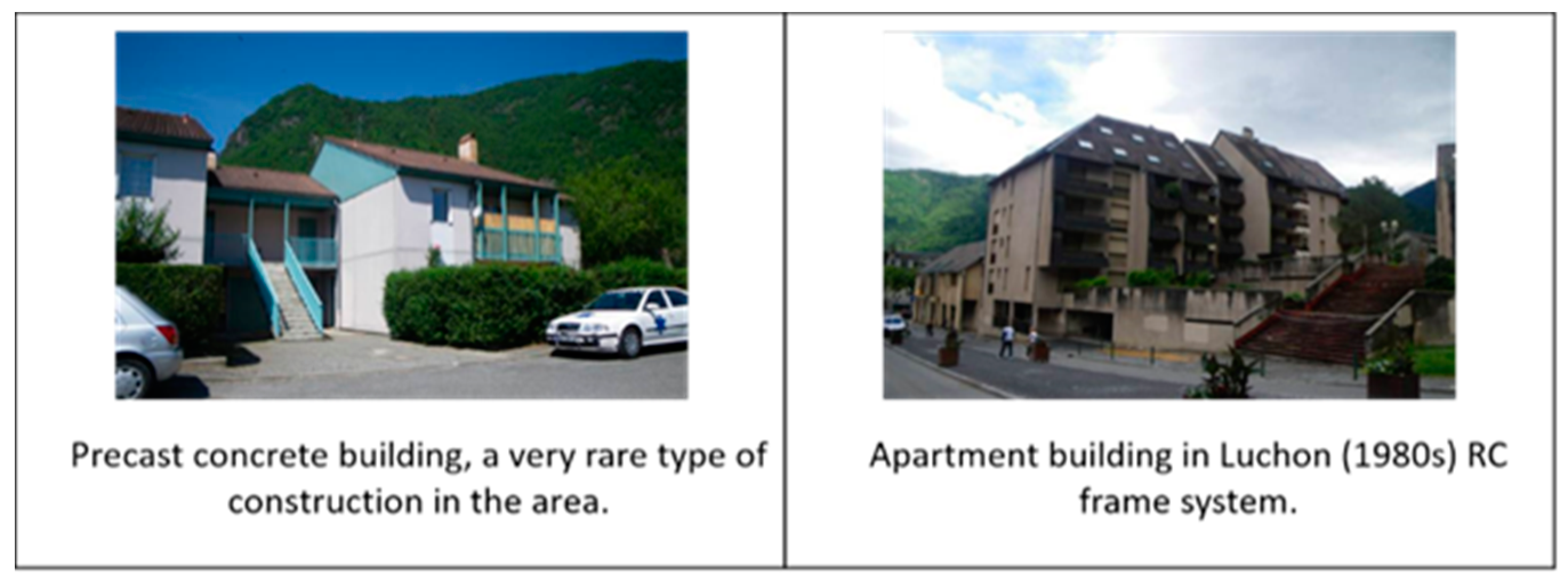
The Luchon area was characterized by a large number of T1- and T1′-type buildings (stone bearing walls), as the urban growth of these cities over the past 40 years has been very low. These types of stone and brick masonry have connections between perpendicular walls that are not strong enough. Additionally, the connections between wooden-beam slabs and the roof with the bearing walls are also poor. Bagnères-de-Luchon, the most important town, developed especially at the start of the 20th century, in association with thermal tourism. The new constructions in this area (in the 1960s and 1970s) are mainly residential neighborhoods (T2 and T3) (Figure A2 in Appendix A), with few apartment blocks having been built (T4 and T5) (Figure A3 in Appendix A). In such areas, with moderate seismicity, other important aspects of vulnerability must be taken into account, such as the non-structural elements of buildings.

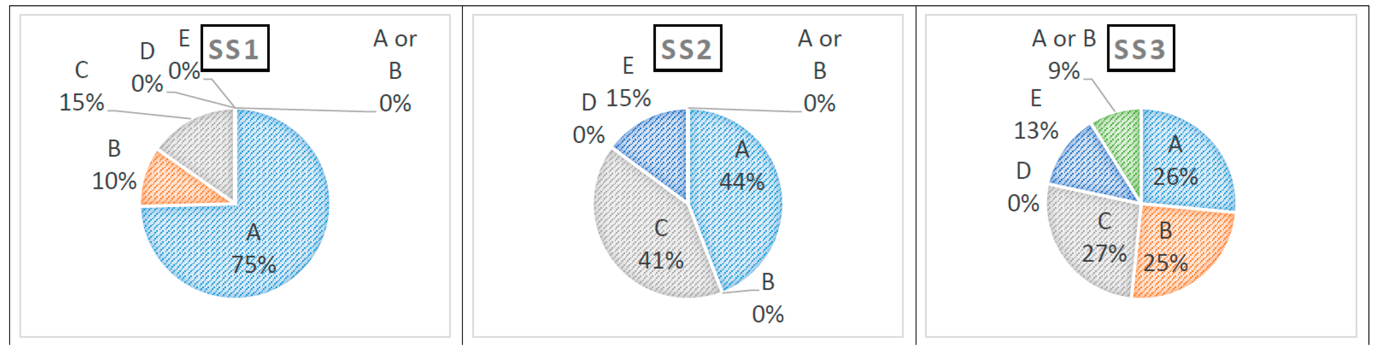
4.4. Harmonizing Vulnerability Indices from Different Exposure Databases

The fragility of residential buildings to earthquake shaking can be characterized by the vulnerability indices (Vi), which range from zero (no vulnerability to earthquake shaking) to one (building is highly vulnerable to shaking). The exposure data for the three scenarios, in terms of number of buildings per municipality and the corresponding average vulnerability indices, are presented in Table 5. Looking at the vulnerability indices for the three datasets, we can notice that the three average values were quite similar, with a small decrease of the average value with the increase of the characteristics describing the typologies. A first observation is that, in this specific case, the European and Regional databases were on the safe side, with higher vulnerability indices than those determined from the Local database. A second observation from Table 5 is that the variation in the vulnerability indices was smaller for the Local database, with respect to the Regional Database, and almost equivalent to that of the European Database.

5. Results and Discussion

5.1. Damage Estimation for the Hazard of pga = 200 cm/s2 (on Rock Conditions)

First, we observed the results for the simulations with a constant moderate ground acceleration of 200 cm/s2 applied to the buildings, without considering the local soil effect (Figure 4). Scale scenario 1 (SS1) showed that 11.5% of the buildings would face heavy damage to complete collapse (D3, D4, and D5). On the other hand, scale scenarios 2 (SS2) and 3 (SS3) showed similar estimates for the heavy to complete damage of the buildings (8.14% and 8.24%, respectively). We can conclude that the large-scale European building characterization overestimated the estimation of heavy damages to buildings by a factor of 1.4, compared to the National statistics database and the in-situ collected database. We also observed that SS2 estimated more undamaged buildings, D0 (a difference of 5%), than SS1 and SS3. These observations, resulting from the simulation run without considering site effects, are coherent with the observations related to the vulnerability indices shown in Table 5 as, in these estimates, the damage calculations were solely influenced by the vulnerability descriptions of the buildings: SS1 showed the largest average vulnerability values; however, SS2 showed the largest variability for the vulnerability.
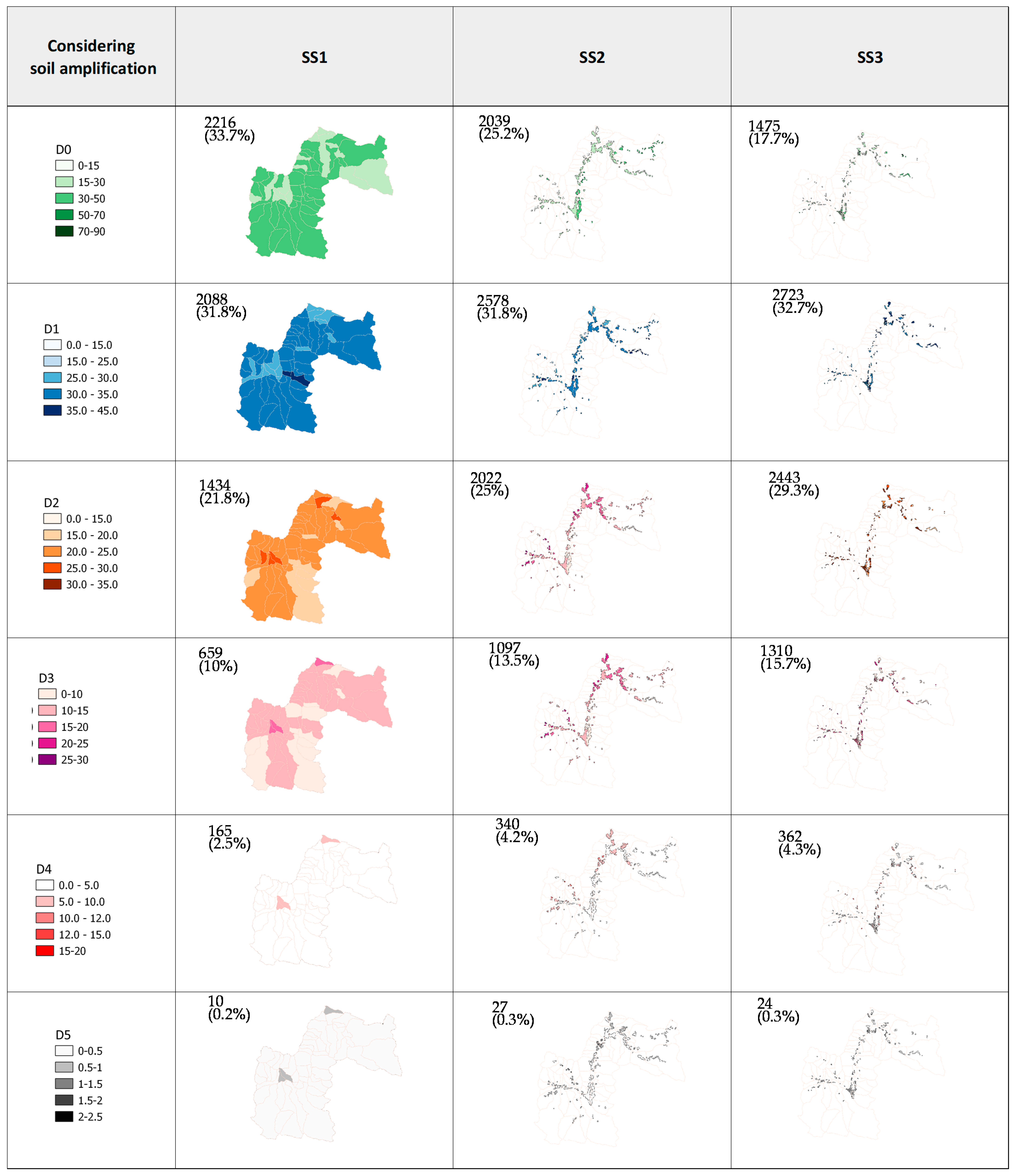
Next, we observed the results of the simulations computed for the three scale scenarios, where the ground motion was amplified by the corresponding site amplification factors (Figure 5). SS1 (using the European soil map with an amplification factor up to 1.5 and the European exposure database) showed that 12.7% of buildings would face heavy damage to complete collapse, versus 18% following SS2 (using the regional soil map with an amplification factor up to 1.8 and the National statistics database) and 20.3% following SS3 (using the local soil map with an amplification factor up to 1.8 and the field-investigation database). The impact of the soil conditions was not linear/translational. We noted that the low resolution of the European soil map in SS1 barely changed the results when comparing the results with and without consideration of the soil amplification map, with a difference factor of only 1.1. This factor was about 2.2 and 2.5, respectively, for SS2 and SS3. Thus, SS1 highly underestimated the proportion of heavily damaged to collapsed buildings (D3–D5). Even though SS3 had the lowest vulnerability indices, it estimated the largest damages, due to the site effects highly amplifying the local ground motion at buildings.
An important increase of severe damage (D5) was observed for the three different scale scenarios when comparing the computations with and without soil amplification: when considering the soil maps using SS1, 4 additional buildings completely collapsed, versus 24 additional buildings for SS2 and 21 for SS3. This result cannot be extrapolated, as such, to some other regions and areas, as it is very dependent on the local geology.
Bal et al. [15] studied the geographical resolution of exposure data and of the ground motion (PGA amplified by the soil effect) for the sea of Marmara region in Turkey, using several different levels of spatial aggregation to estimate the losses due to a single earthquake scenario. They showed that, if only mean estimates are needed, the effort required to refine the spatial definition of exposure data is not justified. The average damage values over the simulations were almost insensitive to the resolution of the ground motion field. Their results indicated that a significant reduction in the variability of these estimates can be achieved by moving to higher resolution ground-motion fields. As the effect of moving to higher resolutions is to introduce some regions with higher-than-average damage and others with lower-than-average damage, these two effects largely cancel each other out.
For the Luchon area and for moderate earthquakes, we conclude that SS1 overestimated the heavy damages, when considering the building database only, and underestimated the heavy damages, when additionally considering the soil characterization maps. We also conclude that SS2 and SS3 generated comparable results, in terms of heavy damages.
These results are in accordance with [21], who mentioned that the loss estimates become accurate and stable beyond a certain (fine) spatial resolution. They also proposed that a potential way to reduce this type of uncertainty is by improving the detail of information, concerning the location of the building inventory; however, this process can be time- and resource-demanding and, in many cases, it is simply impractical (e.g., for risk analysis at the national level). Dabbeek and Silva [69] recommended effective alternatives, involving the disaggregation of the exposure in each unit using night-time lights, satellite imagery, or the location of roads.
When we compare the simulations of the three datasets at the municipality level, the results were quite consistent; however, if we are interested in the infra-municipality level, better resolution of the building data can provide some information about the spatial distribution of damage inside a municipality.
We note that more outliers (or extreme values) were present for SS1 and SS2 than for SS3, where the latter database was collected from field inspections. The percentage of damages D3–D5 was, however, more uniformly distributed for SS3, compared to SS2 (for which the values of Vi were more variable). Pittore et al. [22] concluded that an adaptive model is favorable, with higher spatial resolution in highly urbanized areas (where most of the assets are located) and lower resolution in rural, less-inhabited regions (where higher spatial aggregation could increase the robustness of the risk estimates).
When we consider the total amount of damages in the area, the difference in the heavy damage degree (D3) should be an important issue from the emergency management point of view, as this damage degree implies heavy structural damages and generally inhabitable buildings before inspection. In addition, these levels of damage can also result in road closures, which can have a very significant impact in terms of the routing of emergency resources as well as the evacuation of victims. Figure 6 presents the results of SS3, in terms of the percentage of heavily damaged buildings (≥D3), represented at the municipality (as for the scenarios SS1 and SS2) and infra-municipality levels (homogeneous vulnerability census block). Figure 7 supports Figure 6, with numerical values for the three most populated municipalities (31500, 31360, and 31244) around the main municipality (31042; Bagnères de Luchon).

5.2. Application to Two Historical Earthquakes

Several destructive earthquakes have occurred in the past around the Luchon area, as evidenced by the historical seismicity database SISFRANCE (BRGM-EDF-IRSN: www.sisfrance.net, accessed on 1 March 2021; [70]); including, in particular, two earthquakes that occurred in the 19th century—in 1855 and then in 1870—with an epicentral macroseismic intensity of VII, felt in the Luchon valley with maximum macroseismic intensities of VII and VI, respectively. However, the most important recent regional earthquake remains that of Viella, which occurred on November 19, 1923, in Spain in the Aran Valley, with an epicentral macroseismic intensity of VIII, felt with a macroseismic intensity of VII in the Luchon valley: in Bagnères-de-Luchon, some walls, chimneys, and roofs had cracked. Considering the epicentral positions and the macroseismic intensity level in the area of interest, we evaluated the seismic damage in the Luchon region for the two historical earthquakes (i.e., those of 1855 and 1923). Utilizing the characteristics of these two earthquakes (location, magnitude, and depth) determined by [71] in their FCAT-17 parametric catalog (Table 6), we use the GMPE of [72] to estimate the ground motion in the region, in terms of PGA (Figure 8a,b). Then, the PGA estimated under rock site conditions was convoluted with site effects, following the three soil characterization maps corresponding to each of the three scale scenarios. The resulting PGA maps are shown in Figure 8c,e,g and Figure 8d,f,h for the two earthquakes, respectively, and the corresponding damages were computed.
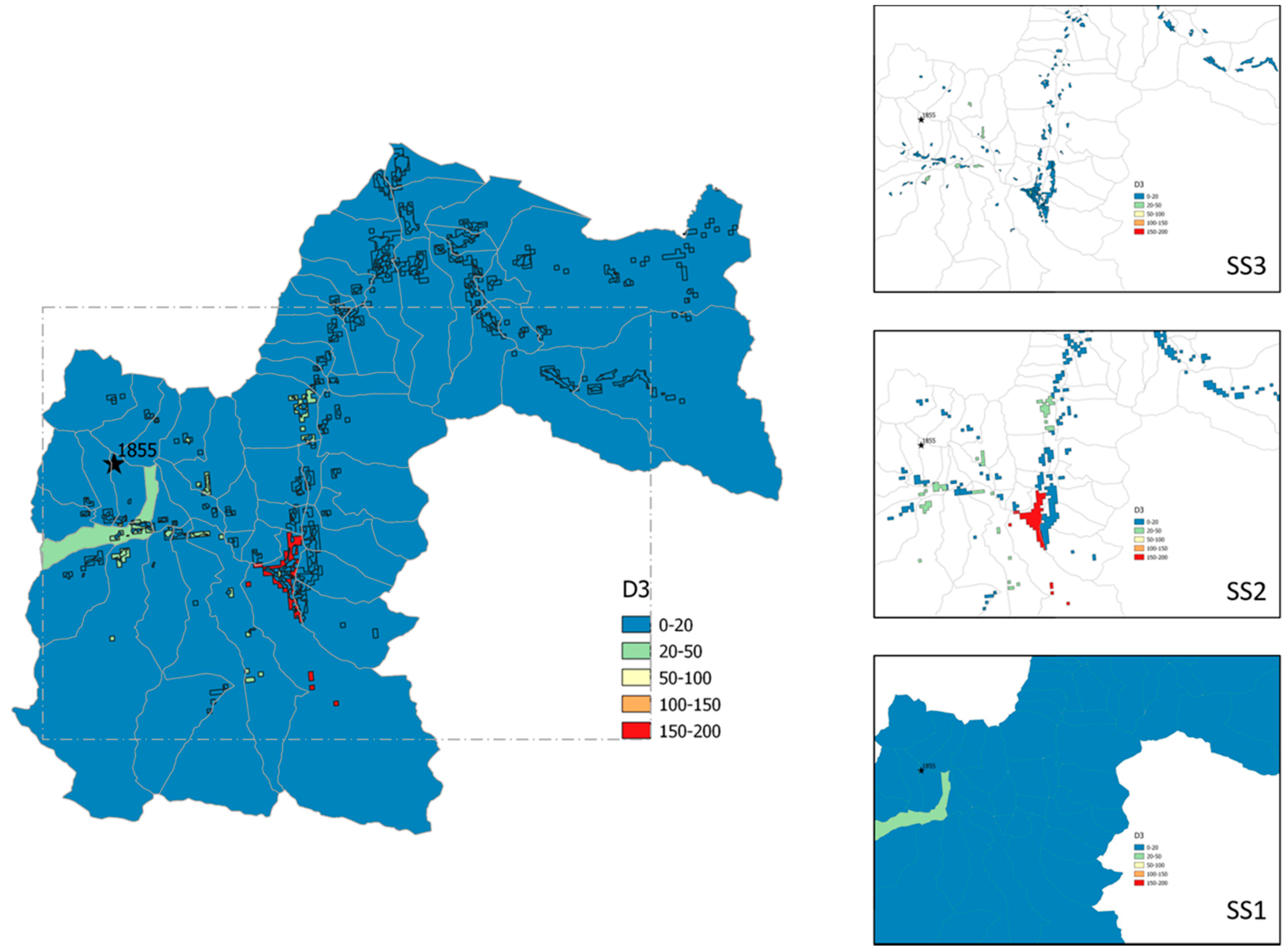
Concerning the 1855 earthquake (Table 7), due to the proximity of the epicenter to the study area, high PGA values were obtained, resulting in damages up to D4 and D5. The distribution of the damage differed from one scenario to another and it was very sensitive to the soil characterization map, as well as to the resolution of the building distribution. Without considering site effects, SS1 generated higher D5 damages (almost double, compared to SS1 and SS2) and less D2–D3 damages, whereas SS2 and SS3 exhibited a similar distribution of damages. When considering the amplified ground motion due to site effects, the conclusions were reversed: SS2 and SS3 generated considerably more damages at levels D3–D5. 
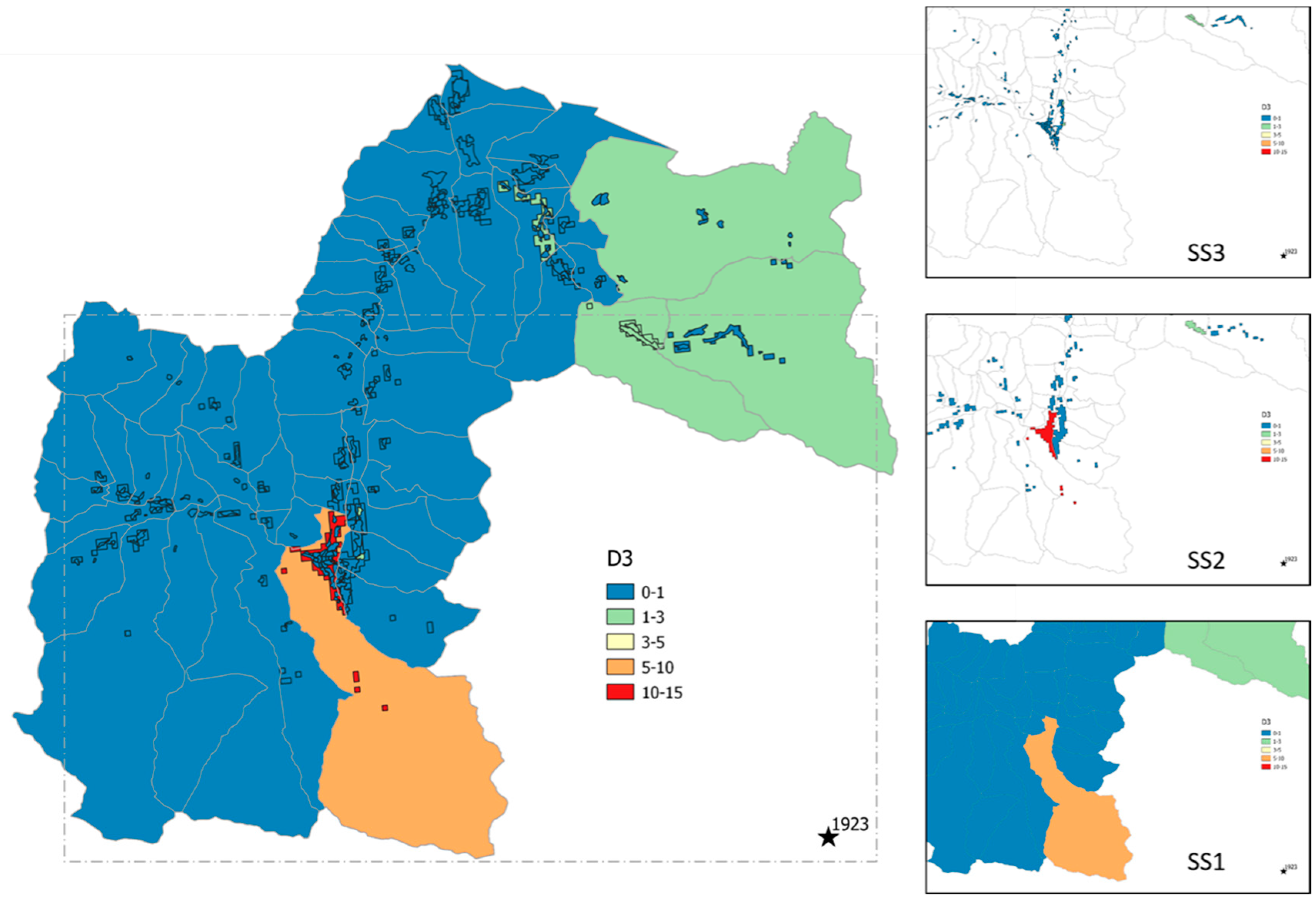
Figure 9 shows the spatial distribution of damaged buildings at level D3. Here, we focused on the Bagnères-de-Luchon municipality, where important differences appeared: only 10 buildings were expected to have D3 damage in this area when using SS1; however, 195 buildings were expected to have D3 damage when using SS2, and 190 in total with SS3, which were spatially dispersed.
For the event of 1923 (Table 8), the epicenter being further away from the study area, low to moderate levels of PGA gave rise to relatively similar distributions of damage. Damages were dominated by levels ranging from D0 to D3. Without considering any soil amplification, SS1 scenarios were the most conservative, whereas SS2 and SS3 generated a similar distribution of damages. When considering the amplified ground motion, this observation did not hold and SS3, followed by SS2, was slightly more conservative. Through observation of Figure 10, which shows the spatial distribution of D3 for the three scale scenarios in the municipality of Bagnères-de-Luchon, we can estimate that six buildings reached damage level D3 using SS1, and 11 buildings using SS2; however, checking SS3 at the infra-municipality level, we can notice that the buildings with damage D3 are spatially distributed with unit values. When collectively aggregated at the municipality level, the number rose to 10. SS2 and SS3 gave similar results.
We can notice that, for the two studied events, the site effect had a large impact on the proportion of destructive damage, and SS2 and SS3 resulted in similar damage distribution estimates, with SS3 having a better spatial resolution of the building locations on the map. However, as this comparison is not based on damage observations, this study is not a validation of damage predictions, but rather an illustration of the variations expected in terms of loss assessment in the event of a major earthquake.

5.3. Impact on the Use of Damage Scenarios for Earthquake Crisis Management

Damage scenarios are useful tools in different phases of seismic risk management, from the preventive “inter-event” phase to the post-seismic phase of crisis management, including for (note that this is a non-exhaustive list):
  • Pre-earthquake phases:
    Awareness of local institutions and population about seismic risk;
    Preparation for crisis management through the development of plans and performing exercises; and
    Identification of the zones where supplementary risk studies are needed.
  • Post-earthquake phases:
    Decision support for crisis management practitioners, mainly for civil protection services; and
    Estimation of economic losses following the occurrence of an earthquake.
Besides the common interest in realistic damage assessment scenarios, each particular use corresponds to a different level of required precision, which may justify the use of more- or less-resolved input data. Regarding the specific issue of crisis management, Table 9 identifies the diversity of these requirements and the corresponding impact on the expected resolution of the damage assessments. This table suggests that intermediate-scale scenarios (e.g., SS2) are likely sufficient to meet a number of needs, for which the effort of acquiring very precise data (e.g., SS3) may not be justified. However, this discussion deserves to be conducted at the scale of a territory, on the basis of a broad analysis of needs, and including relevant stakeholders. Indeed, as soon as a single need justifies the acquisition of precise local data, it becomes relevant to use them for all damage scenarios carried out in this territory.
It is worth noting that the construction of loss scenarios useful for crisis management purposes is not limited to the building damage assessment considered in this paper, but may include consideration about the potential for induced effects such as landslides or soil liquefaction [73], functional losses resulting from structural damage [74], or potential domino effects that could lead to NaTech events [75]. The assessment of building damage is therefore only one of the central steps in a broader process of qualifying the resilience of systems to earthquakes [76].

5.4. Impact on the Use of damage Scenarios for Earthquake Crisis Management

Damage scenarios are useful tools at different phases of seismic risk management, from the preventive “inter-event” phase, to the post-seismic phase of crisis management, such as (non-exhaustive list):
  • Pre-earthquake phases:
    Awareness of local institutions and population about seismic risk;
    Preparation for crisis management through the development of plans and performing exercises;
    Identification of the zones where supplementary risk studies are needed.
  • Post-earthquake phases:
    Decision support for crisis management practitioners, mainly for civil protection services;
    Estimation of economic losses following the occurrence of an earthquake.
Behind a common interest in realistic damage assessment scenarios, each particular use corresponds to a different level of needed precision, which may justify the use of more or less resolved input data. Regarding the specific issue of crisis management, Table 9 identifies the diversity of these needs, and the corresponding impact on the expected resolution of the damage assessments. This table suggests that intermediate scale scenarios (e.g., SS2) can probably be enough to meet a number of needs, for which the effort of acquiring very precise data (e.g., SS3) may not be justified. However, this discussion deserves to be conducted at the scale of a territory on the basis of a broad analysis of needs with relevant stakeholders. Indeed, as soon as a single need justifies the acquisition of precise local data, it becomes relevant to use them for all the damage scenarios carried out on this territory.

6. Conclusions

A major source of uncertainty in damage estimations is the intrinsically difficult inventory problem. Despite these limitations, it is important to thoroughly document the manner in which the inventories were established and damages were estimated, and that the main findings and conclusions are presented in a way that is useful and clear. Seismic damage studies which are properly conducted and used with an understanding of the strengths and limitations of the used method(s) can be of great value in planning, initiating, and updating programs for earthquake risk reduction and in emergency planning.
This paper explored the impact of the resolution of both the ground motion field due to the soil effect and building exposure data on the estimation of seismic damages. The study was limited necessarily to a single seismic ground shaking affecting the region, and the damage calculations were carried out using only one methodology.
For the Luchon area and for moderate earthquakes, the use of the European soil map (with an amplification factor up to 1.5) and the European building database led to an underestimation of the heavy damage classes (D3–D5). Using the regional soil map (with an amplification factor up to 1.8) and the National statistics building database resulted in similar estimates to those using the local soil map (with an amplification factor up to 1.8) and a field-investigation database for the buildings; however, the spatial resolution to detect the locations of buildings of interest was unsurprisingly better when using the better-resolved exposure database. We would like to highlight that the main conclusions from this study are valid for the case of the Luchon area and, as such, their application to other countries or cities should be carefully considered.

Author Contributions

Conceptualization, R.F. and C.N.; methodology, software, validation, formal analysis, investigation, R.F., C.N. and A.R.; resources and data curation, C.N., A.R. and M.F.; writing—original draft preparation, R.F.; writing—review, editing and visualization R.F., C.N., S.A., P.G.; supervision, R.F.; project administration, P.G.; funding acquisition, P.G.; All authors have read and agreed to the published version of the manuscript.

Funding

This research was funded by the European Union’s Horizon 2020 research and innovation programme under grant agreement Turnkey No 821046.

Data Availability Statement

BSS: http://infoterre.brgm.fr/, accessed on 1 March 2021.

Acknowledgments

The authors are grateful for the support of the GEM Foundation, Jamal al Dabbeek and Helen Crowley, who provided the building exposure data from the SERA project.

Conflicts of Interest

The authors declare no conflict of interest. The funders had no role in the design of the study; in the collection, analyses, or interpretation of data; in the writing of the manuscript, or in the decision to publish the results.

INSEE Statistic Database

www.insee.fr, accessed on 1 March 2021.

Sisfrance Historical Database (BRGM-EDF-IRSN)

https://sisfrance.irsn.fr/, accessed on 1 March 2021.

ESRM20

Hazard and risk model data will be available in 2021 on EFEHR portal www.efehr.org/e, accessed on 1 March 2021.

Icelandic Institute of Natural History

https://en.ni.is/, accessed on 1 March 2021.

SISPyr

http://www.sispyr.eu/, accessed on 1 March 2021.

SERA Project Deliverables

Vigirisks Platform

https://vigirisks.net/, accessed on 1 March 2021.

Appendix A

Figure A1. Examples of the main building types found in Bagnères-de-Luchon sector.
Geosciences 11 00249 g0a1
Figure A2. Residential neighborhoods and urbanizations (type T2 and T3) in the Luchon area constructed around the 1960s and 1970s.
Geosciences 11 00249 g0a2
Figure A3. Apartment blocks (type T4 and T5) in the Luchon area constructed around the 1960s and 1970s.
Geosciences 11 00249 g0a3

References

  1. Corbane, C.; Hancilar, U.; Ehrlich, D.; De Groeve, T. Pan-European seismic risk assessment: A proof of concept using the Earthquake Loss Estimation Routine (ELER). Bull. Earthq. Eng. 2017, 15, 1057–1083. [Google Scholar] [CrossRef]
  2. Dolce, M.; Prota, A.; Borzi, B.; Da Porto, F.; Lagomarsino, S.; Magenes, G.; Moroni, C.; Penna, A.; Polese, M.; Speranza, E.; et al. Seismic risk assessment of residential buildings in Italy. Bull. Earthq. Eng. 2020, 1–34. [Google Scholar] [CrossRef]
  3. Silva, V.; Amo-Oduro, D.; Calderon, A.; Costa, C.Q.M.; Dabbeek, J.; Despotaki, V.; Martins, L.; Pagani, M.; Rao, A.; Simionato, M.; et al. Development of a global seismic risk model. Earthq. Spectra 2020, 36, 372–394. [Google Scholar] [CrossRef]
  4. Crowley, H.; Despotaki, V.; Rodrigues, D.; Silva, V.; Toma-Danila, D.; Riga, E.; Karatzetzou, A.; Fotopoulou, S.; Zugic, Z.; Sousa, L.; et al. Exposure model for European seismic risk assessment. Earthq. Spectra 2020, 36, 252–273. [Google Scholar] [CrossRef]
  5. Riga, E.; Karatzetzou, A.; Apostolaki, S.; Crowley, H.; Pitilakis, K. Verification of seismic risk models using observed damages from past earthquake events. Bull. Earthq. Eng. 2021, 19, 713–744. [Google Scholar] [CrossRef]
  6. Cacace, F.; Zuccaro, G.; De Gregorio, D.; Perelli, F.L. Building Inventory at National scale by evaluation of seismic vulnerability classes distribution based on Census data analysis: BINC procedure. Int. J. Disaster Risk Reduct. 2018, 28, 384–393. [Google Scholar] [CrossRef]
  7. Guérin-Marthe, S.; Gehl, P.; Fayjaloun, R.; Caterina, N.; Auclair, S. Rapid earthquake response: The state-of-the art and recommendations with a focus on European systems. Int. J. Disaster Risk Reduct. 2020, 101958. [Google Scholar] [CrossRef]
  8. Erdik, M.; Sesetyan, K.; Demircioglu, M.; Hancilar, U.; Zulfikar, C.; Cakti, E.; Kamer, Y.; Yenidogan, C.; Tuzun, C.; Cagnan, Z.; et al. Rapid earthquake hazard and loss assessment for Euro-Mediterranean region. Acta Geophys. 2010, 58, 855–892. [Google Scholar] [CrossRef]
  9. Calvi, G.M.; Pinho, R.; Magenes, G.; Bommer, J.J.; Restrepo-Vélez, L.F.; Crowley, H. Development of Seismic Vulnerability Assessment Methodologies over the Past 30 Years. ISET J. Earthq. Technol. 2006, 43, 75–104. [Google Scholar]
  10. Pittore, M.; Haas, M.; Megalooikonomou, K. Risk-Oriented, Bottom-Up Modeling of Building Portfolios With Faceted Taxonomies. Front. Built Environ. 2018, 4, 41. [Google Scholar] [CrossRef]
  11. Goda, K.; Tesfamariam, S. Financial risk evaluation of non-ductile reinforced concrete buildings in eastern and western Canada. Int. J. Disaster Risk Reduct. 2019, 33, 94–107. [Google Scholar] [CrossRef]
  12. Goda, K.; Wilhelm, K.; Ren, J. Relationships between earthquake insurance take-up rates and seismic risk indicators for Canadian households. Int. J. Disaster Risk Reduct. 2020, 50, 101754. [Google Scholar] [CrossRef]
  13. Hofer, L.; Zanini, M.A.; Gardoni, P. Risk-based catastrophe bond design for a spatially distributed portfolio. Struct. Saf. 2020, 83, 101908. [Google Scholar] [CrossRef]
  14. Shahbazi, P.; Mansouri, B.; Ghafory-Ashtiany, M.; Käser, M. Introducing loss transfer functions to model seismic financial loss: A case study of Iran. Int. J. Disaster Risk Reduct. 2020, 51, 101883. [Google Scholar] [CrossRef]
  15. Bal, I.E.; Bommer, J.; Stafford, P.J.; Crowley, H.; Pinho, R.J.S.M. The Influence of Geographical Resolution of Urban Exposure Data in an Earthquake Loss Model for Istanbul. Earthq. Spectra 2010, 26, 619–634. [Google Scholar] [CrossRef]
  16. Falcone, G.; Boldini, D.; Amorosi, A. Site response analysis of an urban area: A multi-dimensional and non-linear approach. Soil Dyn. Earthq. Eng. 2018, 109, 33–45. [Google Scholar] [CrossRef]
  17. Falcone, G.; Acunzo, G.; Mendicelli, A.; Mori, F.; Naso, G.; Peronace, E.; Porchia, A.; Romagnoli, G.; Tarquini, E.; Moscatelli, M. Seismic amplification maps of Italy based on site-specific microzonation dataset and one-dimensional numerical approach. Eng. Geol. 2021, 289, 106170. [Google Scholar] [CrossRef]
  18. Polese, M.; D’Aragona, M.G.; Prota, A. Simplified approach for building inventory and seismic damage assessment at the territorial scale: An application for a town in southern Italy. Soil Dyn. Earthq. Eng. 2019, 121, 405–420. [Google Scholar] [CrossRef]
  19. Crowley, H. Earthquake risk assessment: Present shortcomings and future directions. In Perspectives on European Earthquake Engineering and Seismology; Springer: Cham, Switzerland, 2014; pp. 515–532. [Google Scholar]
  20. Silva, V. Critical Issues in Earthquake Scenario Loss Modeling. J. Earthq. Eng. 2016, 20, 1322–1341. [Google Scholar] [CrossRef]
  21. Kalakonas, P.; Silva, V.; Mouyiannou, A.; Rao, A. Exploring the impact of epistemic uncertainty on a regional probabilistic seismic risk assessment model. Nat. Hazards 2020, 104, 997–1020. [Google Scholar] [CrossRef]
  22. Pittore, M.; Haas, M.; Silva, V. Variable resolution probabilistic modeling of residential exposure and vulnerability for risk applications. Earthq. Spectra 2020, 36, 321–344. [Google Scholar] [CrossRef]
  23. Lagomarsino, S.; Giovinazzi, S. Macroseismic and mechanical models for the vulnerability and damage assessment of current buildings. Bull. Earthq. Eng. 2006, 4, 415–443. [Google Scholar] [CrossRef]
  24. BRGM. Zonage Sismique de la France. Available online: http://www.planseisme.fr/Zonage-sismique-de-la-France.html (accessed on 15 December 2019).
  25. Grünthal, G. European Macroseismic Scale 1998. European Seismological Commission (ESC), 1998. Available online: https://www.gfz-potsdam.de/en/section/seismic-hazard-and-risk-dynamics/projects/previous-projects/seismic-vulnerability-risk-intensity-scales/ems-98-european-macroseismic-scale-1998/ (accessed on 1 May 2021).
  26. Atkinson, G.M.; Sonley, E. Empirical relationships between modified Mercalli intensity and response spectra. Bull. Seismol. Soc. Am. 2000, 90, 537–544. [Google Scholar] [CrossRef]
  27. Sedan, O.; Negulescu, C.; Terrier, M.; Roulle, A.; Winter, T.; Bertil, D. Armagedom-A Tool for Seismic Risk Assessment Illustrated with Applications. J. Earthq. Eng. 2013, 17, 253–281. [Google Scholar] [CrossRef]
  28. Tellez-Arenas, A.; Hohmann, A.; Quentin, A.; Negulescu, C.; Smaï, F. A Web Platform for Storing, Sharing and Executing Scientific Workflows for Natural Risk Assessment: Part 2—Description of an Interoperable Architecture Based on open-Source Components; EGU General Assembly: Vienne, Austria, 2019; pp. 2019–7800. [Google Scholar]
  29. Negulescu, C.; Benaïchouche, A.; Lemoine, A.; Le Roy, S.; Pedreros, R. Adjustability of exposed elements by updating their capacity for resistance after a damaging event: Application to an earthquake–tsunami cascade scenario. Nat. Hazards 2020, 104, 753–793. [Google Scholar] [CrossRef]
  30. Crowley, H.; Weatherill, G.; Riga, E.; Pitilakis, K.; Roullé, A.; Tourlière, B.; Lemoine, A.; Gracianne Hidalgo, C. Delivrable SERA: D26.4 Methods for Estimating Site Effects in Risk Assessments; SERA: Zurich, Switzerland, 2019. [Google Scholar]
  31. Monfort, D.; Roullé, A. Estimation Statistique de la Répartition des Classes de sol Eurocode 8 sur le Territoire Français. Phase 1; Rapport Final. Rapport BRGM/RP-66250-FR; BRGM: Orleans, France, 2016; 48p. [Google Scholar]
  32. Roullé, A.; Macau, A.; Figueras, S.; Monfort, D.; Lantada, N.; Susagna, T.; Irizarry, J. Performing seismic scenarios in the Luchon-Val d’Aran area, Central Pyrenees. In Proceedings of the 7th EUropean Congress on REgional GEOscientific Cartography and Information Systems: 7th EUROGEO, Bologne, Italy, 12–15 June 2012. [Google Scholar]
  33. Crowley, H.; Rodrigues, D.; Silva, V.; Despotaki, V.; Romao, X.; Castro, J.M.; Akkar, S.; Hancılar, U.; Pitilakis, K.P.D.; Belvaux, M.; et al. Towards a Uniform Earth-Quake risk Model for Europe. In Proceedings of the 16th European Conference on Earthquake Engineering, Thessaloniki, Greece, 18–21 June 2018. [Google Scholar]
  34. Sedan, O.; Terrier, M.; Negulescu, C.; Winter, T.; Roullé, A.; Douglas, J.; Rohmer, J.; Bes-de-Berc, S.; De Martin, F.; Arnal, C.; et al. Scénario Départemental de Risque Sismique-Méthodologie et Processus de Réalisation. Rapport BRGM/RP-55415-FR, 459p, 96 fig, 45 tabl, 25 Annexes, 2008 France. Available online: https://side.developpement-durable.gouv.fr/PAE/doc/SYRACUSE/86214 (accessed on 5 June 2021).
  35. Monfort, D.; Negulescu, C.; Roullé, A.; Colas, B.; Lantada, N.; Valcarcel, J.; Rodriguez, J.; Pujades, L.; Barbat, A.; Irizarry, J.; et al. Seismic risk scenarios in a cross-border zone of the Pyrenees Pyrenees. In Proceedings of the 15th World Conference on Earthquake Engineering (WCEE), Lisboa, Portugal, 24–28 September 2012. [Google Scholar]
  36. Eurocode, C.E.N. 8: Design Provisions for Earthquake Resistance of Structures–Part 1: General Rules, Seismic Actions and Rules for Buildings; European Committee for Standardization: Brussels, Belgium, 2004. [Google Scholar]
  37. Falcone, G.; Mendicelli, A.; Mori, F.; Fabozzi, S.; Moscatelli, M.; Occhipinti, G.; Peronace, E. A simplified analysis of the total seismic hazard in Italy. Eng. Geol. 2020, 267, 105511. [Google Scholar] [CrossRef]
  38. Wills, C.J.; Clahan, K.B. Developing a map of geologically defined site-condition categories for California. Bull. Seismol. Soc. Am. 2006, 96, 1483–1501. [Google Scholar] [CrossRef]
  39. Lee, C.-T.; Tsai, B.-R. Mapping Vs30 in Taiwan. Terr. Atmospheric Ocean. Sci. 2008, 19, 6. [Google Scholar] [CrossRef] [Green Version]
  40. McPherson, A.; Hall, L. Site Classification for Earthquake Hazard and Risk Assessment in Australia. Bull. Seism. Soc. Am. 2013, 103, 1085–1102. [Google Scholar] [CrossRef]
  41. Di Capua, G.; Peppoloni, S.; Amanti, M.; Cipolloni, C.; Conte, G. Site classification map of Italy based on surface geology. Geol. Soc. Lond. Eng. Geol. Spéc. Publ. 2016, 27, 147–158. [Google Scholar] [CrossRef]
  42. Wald, D.J.; Allen, T.I. Topographic Slope as a Proxy for Seismic Site Conditions and Amplification. Bull. Seism. Soc. Am. 2007, 97, 1379–1395. [Google Scholar] [CrossRef] [Green Version]
  43. Allen, T.I.; Wald, D.J. On the Use of High-Resolution Topographic Data as a Proxy for Seismic Site Conditions (VS30). Bull. Seism. Soc. Am. 2009, 99, 935–943. [Google Scholar] [CrossRef]
  44. Mori, F.; Gena, A.; Mendicelli, A.; Naso, G.; Spina, D. Seismic emergency system evaluation: The role of seismic hazard and local effects. Eng. Geol. 2020, 270, 105587. [Google Scholar] [CrossRef]
  45. Stewart, J.P.; Afshari, K.; Hashash, Y.M. Guidelines for performing hazard-consistent one-dimensional ground response analysis for ground motion prediction. PEER Rep. 2014, 16, 117. [Google Scholar]
  46. Crowley, H.; Silva, V.; Kalakonas, P.; Martins, L.; Weatherill, G.; Pitilakis, K.; Riga, E.; Borzi, B.; Faravelli, M. Verification of the European Seismic Risk Model (ESRM20). In Proceedings of the 17th World Conference on Earthquake Engineering, Sendai, Japan, 13–18 September 2020. [Google Scholar]
  47. Roullé, A.; Auclair, S.; Dewez, T.; Hohmann, A.; Lemoine, A.; Rey, J. Cartographie Automatique des Classes de sol à l’échelle Régionale à Partir d’un Modèle Numérique de Terrain ou de Surface. Rapport Final. 2010, pp. 1–66. Available online: https://www.researchgate.net/publication/278736397_Cartographie_automatique_des_classes_de_sol_a_l’echelle_regionale_a_partir_d’un_modele_numerique_de_surface (accessed on 1 March 2021).
  48. Lemoine, A.; Douglas, J.; Cotton, F. Testing the Applicability of Correlations between Topographic Slope and VS30 for Europe. Bull. Seism. Soc. Am. 2012, 102, 2585–2599. [Google Scholar] [CrossRef] [Green Version]
  49. Vilanova, S.P.; Narciso, J.; Carvalho, J.P.; Lopes, I.; Quinta-Ferreira, M.; Pinto, C.C.; Nemser, E.S. Developing a Geologically Based VS30 Site-Condition Model for Portugal: Methodology and Assessment of the Performance of Proxies Developing a Geologically Based VS30 Site-Condition Model for Portugal. Bull. Seismol. Soc. Am. 2018, 108, 322–337. [Google Scholar] [CrossRef]
  50. Cassard, D.; Bertrand, G.; Billa, M.; Serrano, J.-J.; Tourlière, B.; Angel, J.-M.; Gaál, G. ProMine Mineral Databases: New Tools to Assess Primary and Secondary Mineral Resources in Europe. In Mineral Deposits of North Africa; Springer Science and Business Media LLC: Berlin/Heidelberg, Germany, 2015; pp. 9–58. [Google Scholar]
  51. Johannesson, H. Geological Map of Iceland-1/600 000-Bedrock Geology; Icelandic Institute of Natural History: Gardabaer, Iceland, 2014. [Google Scholar]
  52. Colas, B.; Goula, X.; Roullé, A.; Garcia, I.; Buxo, P.; Roviro, I.; Dewez, T.; Nus, E. SISPyr report R10. Action 4.1: Shake-Map-Site Effect Corrections. 2010. Available online: http://www.sispyr.eu/IMG/pdf/R10-M41-ShakeMap_Site_effect_corrections.pdf (accessed on 5 June 2021).
  53. Colas, B.; García, I.; Buxó, P.; Roullé, A.; Goula, X. Geological based seismic microzonation for Pyrenees. In Proceedings of the 7th EUropean Congress on REgional GEOscientific Cartography and Information Systems: 7th EUROGEO, Bologne, Italy, 12–15 June 2012. [Google Scholar]
  54. Courboulex, S.; Barnolas, A.; Calvet, M.; Martin-Alfageme, S. Carte Géologique du Quaternaire des Pyrénées à 1/400 000 BRGM-ITGE; BRGM: Orléans, France, 2008. [Google Scholar]
  55. Baudin, T.; Barnolas, A.; Gil, I.; Martin-Alfageme, S. Carte Géologique des Pyrénées à 1/400 000 (Socle) BRGM-ITGE; Editions BRGM: Orléans, France, 2008. [Google Scholar]
  56. SISPYR: Sintesi Dels Dipòsits Quaternaries i Cubetes Neògenes en el Sector ibèric (Guipuzcoa, Navarra Atragó i Catalunya). SISPYR Report 2011. Available online: https://pocrisc.eu (accessed on 5 June 2021).
  57. Roullé, A.; Colas, B. SISPyr Report R12b. Action 4.2: Microzonage Sismique de la Vallée de Luchon (France). (In French). 2012. Available online: http://www.sispyr.eu/IMG/pdf/R12b-M42-Microzonage_sismique_de_la_vallee_de_Luchon.pdf (accessed on 5 June 2021).
  58. Mouroux, P.; Le Brun, B. Presentation of RISK-UE Project. Bull. Earthq. Eng. 2006, 4, 323–339. [Google Scholar] [CrossRef]
  59. Kircher, C.A.; Whitman, R.V.; Holmes, W.T. HAZUS Earthquake Loss Estimation Methods. Nat. Hazards Rev. 2006, 7, 45–59. [Google Scholar] [CrossRef]
  60. Federal Emergency Management Agency (FEMA). HAZUS99 Earthquake Loss Estimation Methodology, User Manual; Federal Emergency Management Agency: Washington, DC, USA, 1999. [Google Scholar]
  61. Federal Emergency Management Agency (FEMA). Using HAZUS-MH for Risk Assessment (FEMA 433); Federal Emergency Management Agency: Washington, DC, USA, 2004. [Google Scholar]
  62. Porter, K. Cracking an Open Safe: Uncertainty in HAZUS-Based Seismic Vulnerability Functions. Earthq. Spectra 2010, 26, 893–900. [Google Scholar] [CrossRef]
  63. Silva, V.; Yepes-Estrada, C.; Dabbeek, J.; Martins, L.; Brzev, S. GED4ALL-Global Exposure Database for Multi-Hazard Risk Analysis–Multi-Hazard Exposure Taxonomy; Global Earthquake Model Foundation: Pavia, Italy, 2018. [Google Scholar]
  64. PS 69 (DTU P 06-003). Afnor 1972. Regles Parasismiques 1969 et Annexes. (In French). Available online: https://read-download-books.com/v6/preview/?pid=6&offer_id=26&ref_id=f75a972538ddfd2e453c162772ed4Dh1_d3178de1_c28f910b&sub1=23160&keyword=Regles%20Parasismiques%201969%20Et%20Annexes (accessed on 1 March 2021).
  65. Eyrolles (Ed.) Règles Parasismiques 1969 Révisées 1982 et Annexes (DTU Règles PS 69/82). 1984. Available online: http://www.icab.eu/guide/ps92/ (accessed on 1 March 2021).
  66. PS 92 (DTU NF P06-013). Afnor 1995. Regles de Construction Parasismique-Regles ps Applicables Aux Batiments. (In French). Available online: https://kupdf.net/download/regles-ps-92-dtu-nf-p06-0131_598739f1dc0d600816300d1a_pdf (accessed on 1 March 2021).
  67. Milutinovic, Z.V.; Trendafiloski, G.S. Risk-UE An Advanced Approach to Earthquake Risk Scenarios with Applications to Different European Towns. Contract: EVK4-CT-2000-00014, WP4: Vulnerability of Current Buildings. 2003, pp. 1–111. Available online: http://www.civil.ist.utl.pt/~mlopes/conteudos/DamageStates/Risk%20UE%20WP04_Vulnerability.pdf (accessed on 1 May 2021).
  68. González Díaz, M. Evaluación del Riesgo Sísmico en el Principado de Andorra; Universitat Politècnica de Catalunya: Barcelona, Spain, 2010. [Google Scholar]
  69. Dabbeek, J.; Silva, V. Modeling the residential building stock in the Middle East for multi-hazard risk assessment. Nat. Hazards 2020, 100, 781–810. [Google Scholar] [CrossRef]
  70. Scotti, O.; Baumont, D.; Quenet, G.; Levret, A. The French macroseismic database SISFRANCE: Objectives, resultsand perspectives. Ann. Geophys. 2004, 47, 571–581. [Google Scholar]
  71. Manchuel, K.; Traversa, P.; Baumont, D.; Cara, M.; Nayman, E.; Durouchoux, C. The French seismic CATalogue (FCAT-17). Bull. Earthq. Eng. 2018, 16, 2227–2251. [Google Scholar] [CrossRef]
  72. Ambraseys, N.N.; Douglas, J.; Sarma, S.K.; Smit, P.M. Equations for the Estimation of Strong Ground Motions from Shallow Crustal Earthquakes Using Data from Europe and the Middle East: Horizontal Peak Ground Acceleration and Spectral Acceleration. Bull. Earthq. Eng. 2005, 3, 1–53. [Google Scholar] [CrossRef] [Green Version]
  73. Mori, F.; Mendicelli, A.; Moscatelli, M.; Romagnoli, G.; Peronace, E.; Naso, G. A new Vs30 map for Italy based on the seismic microzonation dataset. Eng. Geol. 2020, 275, 105745. [Google Scholar] [CrossRef]
  74. Gehl, P.; Cavalieri, F.; Franchin, P. Approximate Bayesian network formulation for the rapid loss assessment of real-world infrastructure systems. Reliab. Eng. Syst. Saf. 2018, 177, 80–93. [Google Scholar] [CrossRef]
  75. Kabir, G.; Suda, H.; Cruz, A.M.; Giraldo, F.M.; Tesfamariam, S. Earthquake-related Natech risk assessment using a Bayesian belief network model. Struct. Infrastruct. Eng. 2019, 15, 1–15. [Google Scholar] [CrossRef]
  76. Fontana, C.; Cianci, E.; Moscatelli, M. Assessing seismic resilience of school educational sector. An attempt to establish the initial conditions in Calabria Region, southern Italy. Int. J. Disaster Risk Reduct. 2020, 51, 101936. [Google Scholar] [CrossRef]
Figure 1. (Left) Map of the Luchon valley and the 53 municipalities. (Right) location of the Luchon area overlaid with the French seismic zonation (article D.563-8-1 du code de l’environnement, Ministère de l’Ecologie, du Développement durable, des Transports et du Logement. Map is created with data from published GIS Data Source: [24]).
Geosciences 11 00249 g001
Figure 2. The site characterization maps and the building exposure used for the three scale scenarios defined in this study.
Geosciences 11 00249 g002
Figure 3. Pie charts of the distribution of soil characterization classes in urbanized areas for the three defined scale scenarios.
Geosciences 11 00249 g003
Figure 4. The damage distribution per scale scenario without considering the ground motion amplification due to soil effects. The color shows the percentage of buildings per level of damage. The number shows the total number of damaged buildings.
Geosciences 11 00249 g004
Figure 5. The damage distribution per scale scenario considering the ground motion amplification due to soil effects. The color shows the percentage of buildings per level of damage. The number shows the total number of damaged buildings.
Geosciences 11 00249 g005
Figure 6. Percentage of damage degree superior to D3 for scenario SS3 for pga of 200 cm/s2 amplified by the site effects: representation to the level of the municipality and to the infra-municipality level (homogeneous vulnerability census block).
Geosciences 11 00249 g006
Figure 7. The damage distribution per municipality (last bar chart of each graphic) and per corresponding homogeneous vulnerability census blocks inside each municipality.
Geosciences 11 00249 g007
Figure 8. The ground motion corresponding to the earthquakes of 1855 (left) and 1923 (right): The first row (a,b) shows the ground motion computed at rock site conditions following the GMPE from [72]. The surface ground motion is amplified due to the soil effect using SS1 (c,d), SS2 (e,f) and SS3 (g,h) soil characterization maps.
Geosciences 11 00249 g008
Figure 9. D3 damage distribution in the Luchon area in number of buildings, at the 53 municipalities, due to the 1855 earthquake. The site effect is considered here.
Geosciences 11 00249 g009
Figure 10. D3 damage distribution in the Luchon area in number of buildings at the 53 municipalities, due to the 1923 earthquake. The site effect is considered here.
Geosciences 11 00249 g010
Table 1. Scale scenario description based on the source of databases to characterize the site amplification as well as the building exposure.
Level of DetailNational Statistics DataIn-Situ Investigation Data
Scale ScenarioSS1: EuropeSS2: FranceSS3: Luchon
HazardConversion of the intensity from acceleration
SoilSite effect zonationEuropean Geological mapNational geological mapRegional geological map
Geol map (1/1,000,000)Geol map (1/40,000) + BoreholesGeol map (1/10,000) + boreholes + geophysical measurements
Site effect amplification3 classes (1−1.35−1.5) following EC86 classes (1−1.2−1.35−1.5−1.6−1.8) following EC8 (with three classes only in the area of study)5 classes (1−1.18−1.35−1.5−1.8) following EC8
ExposureInventory and zonationSERAINSEE and soil occupationHomogeneous census block
53 zones (municipalities)53 zones (municipalities)203 zones (infra-municipal districts)
Vulnerability indexVi corresponding to SERA typology based on RISK-UEVi from INSEE statistics (based on age, type, number of floor)Vi from INSEE statistics improved with Field inspection
DamageMethodology [23]: Building Damage using EMS98 intensity-based buildings vulnerability
Table 2. The taxonomies in the Luchon area according to SERA, the corresponding acronym in RISK-UE and the associated Vi. * Vi—vulnerability index.
SERARISK-UE
TaxonomyRISK-UEDescriptionVi *
W/LWALWWood structures0.45
CR/LFLSRC1Concrete shear frames0.44
MCF/LWALM4Reinforced or Confined Masonry Wall0.45
CR/LFINFRC3.2Irregular frames0.52
CR/LDUALRC4RC dual systems, RC frame and walls0.39
CR+PC/LWALRC6Precast concrete frames, concrete shear walls0.54
MUR+ST/LWALM1.1Rubber stone fieldstone0.87
MUR+CL/LWALM1.2Simple stone0.74
Table 3. The vulnerability index for the different taxonomy groups defined in SERA database.
SERA Taxonomy GroupsVi
CR+PC/LWAL+CDN/HBET:3–50.56
CR/LDUAL+CDM/HBET:6-/7.00.45
CR/LDUAL+CDN/HBET:6-0.45
CR+PC/LWAL+CDN/HBET:6-0.60
CR/LFINF+CDL/H:1/4.00.66
CR/LFINF+CDM/H:2/7.00.50
CR/LFINF+CDL/H:2/4.00.66
W/LWAL+CDN/H:10.43
CR/LFINF+CDN/HBET:3–50.54
CR/LFINF+CDM/H:1/7.00.50
MUR+ST/LWAL+CDN/H:20.85
CR/LDUAL+CDL/HBET:3–5/4.00.57
MUR+CL/LWAL+CDN/H:20.72
CR/LDUAL+CDM/HBET:3–5/7.00.41
W/LWAL+CDN/H:20.43
CR/LFLS+CDN/HBET:6-0.50
MUR+CL/LWAL+CDN/H:10.72
CR/LDUAL+CDL/HBET:6-/4.00.61
MUR+ST/LWAL+CDN/H:10.85
CR/LFLS+CDM/HBET:3–5/7.00.46
CR/LFLS+CDL/HBET:3–5/4.00.62
MCF/LWAL+CDL/H:20.53
CR+PC/LWAL+CDN/H:20.52
MCF/LWAL+CDL/H:10.53
CR/LFLS+CDN/HBET:3–50.46
Table 4. Typology of buildings in the study area used in SS3.
TypeResisting SystemType RISK-UEDescription ViAggravating Factors Observed During Field Inspections
New TaxonomyVi (with Aggravating Factors)
T1Simple stone masonryM1.2Stone load-bearing walls, wooden floors. Traditional house0.74T1L0.74
T1M0.78
T1H0.82
T1LAccole0.78
T1MAccole0.82
T1HAccole0.86
T1′M1.2-M1.3Stone bearing walls, ashlar stone elements. Large buildings in Bagnères de Luchon.0.74–0.616T1bL0.74
T1bM0.78
T1bH0.82
T1bLAccole0.78
T1bMAccole0.82
T1bHAccole0.86
T2Unreinforced brick or concrete block masonryM3.3Unreinforced masonry with joists and vault. 0.704T2L0.664
T2M0.704
T2H0.744
T3M3.4Unreinforced masonry. Floors in concrete.0.616T3L0.576
T3M0.616
T3H0.656
T4Reinforce ConcreteRC3.2Irregular RC frame with infilled masonry0.522T4L0.482
T4M0.522
T4H0.602
T5RC2Concrete shear walls0.386T5L0.346
T5M0.386
T5H0.466
T6Steel structuresS3Steel frame with unreinforced masonry infilled walls0.484T6L0.444
T6M0.484
T6H0.564
T7Wood structuresWWooden chalets0.447T7L0.447
T7M0.447
T7H0.447
Table 5. Building exposure data (number of buildings and the average vulnerability index) by municipality in the Luchon area, extracted from the three databases used for this study.
SS1SS2SS3
NumberMunicipalityNameBuildingsViBuildingsViBuildingsVi
131010ANTIGNAC59.340.7270.310.6869.240.62
231015ARGUT-DESSOUS62.070.6774.530.6676.550.62
331017ARLOS107.730.72114.140.7113.830.63
431019ARTIGUE27.30.7235.180.7739.350.69
531040BACHOS33.820.7433.970.730.810.64
631042BAGNERES-DE-LUCHON999.790.671787.080.71860.710.64
731046BAREN12.90.6520.10.614.080.67
831064BENQUE-DESSOUS-ET-DESSUS37.330.7239.250.6544.450.62
931067BEZINS-GARRAUX61.20.6769.090.6666.980.65
1031068BILLIERE24.170.7223.620.6827.930.67
1131081BOURG-D’OUEIL37.770.72320.6835.320.62
1231085BOUTX496.050.71542.470.71520.760.65
1331092BURGALAYS99.420.72110.070.68105.680.61
1431123CASTILLON-DE-LARBOUST55.340.7283.190.6774.020.62
1531125CATHERVIELLE47.990.7352.510.7164.330.65
1631127CAUBOUS14.270.7416.50.7917.940.62
1731129CAZARIL-LASPENES23.30.7127.420.6923.430.62
1831132CAZAUX-LAYRISSE38.860.7343.740.6846.750.62
1931133CAZEAUX-DE-LARBOUST80.740.7285.660.777.750.62
2031139CHAUM143.070.73164.940.67179.280.62
2131142CIER-DE-LUCHON169.570.7193.440.67188.190.62
2231144CIERP-GAUD502.230.72574.220.68603.570.62
2331146CIRES32.360.7137.580.6535.60.62
2431176ESTENOS119.950.73135.840.69127.020.62
2531177EUP115.030.72123.070.68118.630.62
2631190FOS381.080.74388.190.72401.090.6
2731199FRONSAC157.410.72172.510.72187.680.62
2831213GARIN123.170.7143.970.64127.370.64
2931221GOUAUX-DE-LARBOUST57.170.69620.7271.380.69
3031222GOUAUX-DE-LUCHON58.830.71640.6871.490.69
3131235GURAN66.620.73730.7275.120.62
3231242JURVIELLE30.620.7222.750.7823.830.62
3331244JUZET-DE-LUCHON163.820.68232.810.62227.80.65
3431290LEGE38.90.7442.810.7546.30.62
3531298LEZ64.220.7471.450.6869.530.62
3631316MARIGNAC299.970.72336.940.68356.290.64
3731335MAYREGNE53.960.72600.7262.090.62
3831337MELLES183.850.74193.720.73174.250.65
3931360MONTAUBAN-DE-LUCHON157.990.67248.940.65253.420.62
4031394MOUSTAJON72.820.6988.940.6297.590.61
4131404OO84.030.798.680.7109.80.67
4231432PORTET-DE-LUCHON27.660.7230.530.7431.790.62
4331434POUBEAU55.30.761.690.6453.230.67
4431465SACCOURVIELLE22.590.7226.290.7127.030.62
4531470SAINT-AVENTIN131.550.72142.890.72147.440.66
4631471SAINT-BEAT409.870.71368.360.7375.40.62
4731500SAINT-MAMET287.570.664110.66485.640.66
4831508SAINT-PAUL-D’OUEIL60.630.72730.7280.130.67
4931524SALLES-ET-PRATVIEL72.220.7281.910.6588.330.62
5031548SIGNAC47.820.7153.40.7558.380.62
5131549SODE20.730.7321.650.7622.340.62
5231559TR5BONS-DE-LUCHON12.870.7113.890.714.370.62
5331590BINOS27.30.7128.60.7136.680.64
TotalAverageTotalAverageTotalAverage
6572.150.718103.840.6983380.63
Stdv Stdv Stdv
0.02 0.04 0.02
Table 6. Parameters of the 1855 and 1923 historical earthquakes that affected the region of Luchon, from the FCAT-17 parametric catalog [71].
YearLat (deg)Lon (deg)MwDepth (km)
185542.8330.55.412
192342.70.8335.68
Table 7. Percentage and number of residential buildings per damage level per scale scenario and the corresponding ground motion shown in Figure 8, for the earthquake event of 1855.
1855D0D1D2D3D4D5
SS1SS2SS3SS1SS2SS3SS1SS2SS3SS1SS2SS3SS1SS2SS3SS1SS2SS3
%655043212527914184791330.10.40.3
# 4262406535621359203722926081172147125258474581214243103126
Table 8. Percentage and number of residential buildings per damage level per scale scenario and the corresponding ground motion shown in Figure 8, for the earthquake event of 1923.
1923D0D1D2D3D4D5
SS1SS2SS3SS1SS2SS3SS1SS2SS3SS1SS2SS3SS1SS2SS3SS1SS2SS3
% 878583111214233000000000
# 56916857689771210041162147211243213034122000
Table 9. Examples of damage scenarios that need to be related to crisis management activities, with qualitative assessment of corresponding required level of reliability.
Crisis Management ActivityScenario EarthquakeNeedsFiability
GlobalExpected Spatial ResolutionExpected Accuracy of Assessments
Crisis planningFictiveTo get trends regarding the magnitude of the consequences of credible/dimensioning earthquakes, in order to adapt the response capacity, or even to carry out a pre-sectorization of interventionLow to ModerateDue to the fact that the characteristics of the scenario earthquake(s) do not prefigure those of future real earthquakes, the spatial resolution of the scenarios does not need to be very fine (the scale of the municipality can in most cases suffice).Quantitative estimates are considered to be orders of magnitude, with however a more pronounced expectation on the most marked damage levels (D3 to D5) which directly generate the severity of the crisis situation.
Preparing for the crisis (crisis exercises)To get a quantified and spatialized assessment of damages, in order to propose a credible scenario on which to build a realistic exercise to test the crisis management procedures
Rapid responseRealTo get quickly the most precise possible trends in terms of the extent of the consequences of a particular earthquake, so as to size the operational response (including requests for reinforcements), or even help to prioritize the allocation of resources by sector (search and rescue, post-seismic building diagnosis,...)Low to ModerateImmediately after the occurrence of an earthquake, the challenge is to be able to have as quickly as possible (around 30 after the earthquake) a first estimate, while the parameters of the earthquakes are still often uncertain (particularly location and depth). At this time, the required spatial resolution necessary remains moderate.In the first hour after the earthquake, the precision required on the assessments remains moderate. More pronounced expectation on the most marked damage levels (D3 to D5), which directly generates the severity of the crisis situation.
Moderate to HighAs time passes and before the authorities can have a clear vision of the magnitude of the damages on the sole basis of their feedback from the field, there is a need to update the damage scenarios in order to improve their accuracy as much as possible. Widened interest in lower damage levels (D2) to judge the habitability of the building.
Publisher’s Note: MDPI stays neutral with regard to jurisdictional claims in published maps and institutional affiliations.

