Noise, Regression Dilution Bias, and Solar-Wind/Magnetosphere Coupling Studies

Introduction

Solar-wind/magnetosphere coupling is often studied by examining “driver functions” created from multiple solar-wind variables and testing how well the driver functions do in statistically describing the time-dependent activity of the Earth’s magnetosphere-ionosphere system, with that activity typically measured with a single geomagnetic index. Often the goodness of the driver function is measured by the magnitude of the Pearson linear-correlation coefficient between the time-dependent solar-wind driver function and the time-dependent geomagnetic index. Correlation coefficients of 0.5–0.8 are typical.

Associated with the linear correlation, a least-squares linear-regression fit to the geomagnetic-index values as a function of the driver-function values is often made. In a plot (for example, Figure 1)of the geomagnetic index (vertical) versus the solar-wind driver function (horizontal), the least squares fit is based on minimizing the vertical errors from a line on the plot. In a sense, this least-squares linear-regression fit is the best fit for predicting the value of the geomagnetic index (vertical) knowing the value of the driver (horizontal).

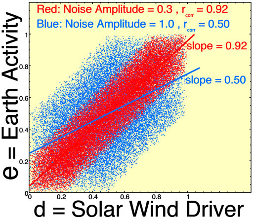
FIGURE 1. A scatterplot of two sets of data (d,e) with two different amounts of noise in the data. Only every 100th data point is plotted.

In this report, artificial data sets are used to explore the effects of noise in the data for the study of solar-wind/magnetosphere coupling. For simplicity and clarity, the artificial data sets employed will not involve time lags as the actual solar-wind and magnetospheric data do.

Regression Dilution Bias

Data that is imperfectly correlated leads to a phenomenon denoted as “regression dilution bias” (e.g., Liu, 1988; Hutcheon et al., 2010) or as “attenuation by errors” (e.g., Spearman, 1904; Bock and Petersen, 1975). Basically, the smaller the Pearson correlation coefficient r_corr, the shallower the slope of the linear regression fit: that is the systematic “bias”. Hence, the larger the noise in the data, the lower the correlation coefficient, and the shallower the slope of the linear-regression fit. Additionally for data points x versus y, the linear-regression fit formula obtained for y(x) (y fitted as a function of x) differs from the fit formula for x(y) (x fitted as a function of y).

In some sense a better fit to the data is a “major-axis linear-regression fit” (Riggs et al., 1978; Warton et al., 2006), also known as a “total least squares fit” (Golub and Van Loan, 1980) or a “Gaussian fit” (Borovsky et al., 1998): this fit minimizes the perpendicular distances to the line rather than just minimizing the vertical distances to the line. If you were to “eyeball” a scatterplot and draw a line through the group of points, your line would approximate the major axis fit and would have a slope steeper than the mathematical linear-regression least-squares fit.

Figure 1 displays some of these concepts with artificial data. Data points e (Earth activity, vertical) are plotted as a function of d (solar wind driver, horizontal). The data sets each are comprised of 300,000 points (d,e), although only every 100th point is plotted. The core data set (d_o,e_o) is not plotted, but it is created as follows. d_o (solar-wind driver) is a box-car distribution of random numbers between 0 and 1. Then e_o (Earth) is created as e_o = d_o. If e_o were to be plotted as a function of d_o, all points would lie on the line e = d, the slope of the linear-regression fit would be 1.0, and the Pearson correlation coefficient would be r_corr = 1.0. The red points in Figure 1 are created by adding noise (boxcar random numbers) to both d_o and e_o where the boxcar noise values go from -0.15 to +0.15. The d and e distributions (d = d_o + noise and e = e_o + noise) are then “standardized” so that they go from values of 0 to values of 1. Similarly the blue points in Figure 1 are created by adding larger-amplitude noise to the d_o and e_o points, where the boxcar noise goes from -0.25 to +0.25, and the distributions are “standardized” after the noise is added. Least-square linear regression fits are performed and plotted as the two lines: a red line for the red points and a blue line for the blue points. For the red points the fit slope is 0.92 and for the more-noisy blue points the fit slope is 0.5. Recall that the “true answer” if there was no noise in the data would be a slope of 1.0. As noted in the scatterplot of Figure 1, with increasing noise the Pearson linear correlation coefficient r_corr is reduced.

If the physics of the solar wind d driving the magnetosphere e is e = d as described by the e_o = d_o points, then noise in the variables in Figure 1 is yielding systematically different formulas for the driving: e = 0.92d and e = 0.5d. With increasing inaccuracy of the data, the interpretation of the fit formulas is that the solar-wind driving of the earth is weaker than it should be: the increase in Earth activity associated with an increase in driving is lessened.

Effect of Noise on a Best-Fit Formula

The solar-wind driver functions are mathematical combinations of solar wind variables. The functional forms used are most often multiplicative combinations of solar-wind variables with non-unity exponents on some of the variables (cf. Table 1 of Baker, 1986, Table 1 of Newell et al., 32,007, Table 1 of Balikhin et al., 2010, Table 1 of Borovsky, 2013), or they can be linear combinations of solar wind variables (Borovsky and Denton, 2018; Borovsky, 2021), or they can be time integrals of solar-wind variables (Borovsky, 2017). We don’t know the “correct” functional form of the solar-wind driver function for the Earth, so we often look for the solar-wind function that gives the best correlation with geomagnetic indices (e.g., Newell et al., 2007; Borovsky, 2014; McPherron et al., 2015). Let’s ask whether noise in the data changes those combinations, i.e., whether noise changes the functional form of a best-fit solar-wind formula to describe the Earth activity.

For a mathematical gedanken experiment, let’s suppose we know how the driving works and can describe it with a solar wind formula. Figure 2 explores how noise in the solar-wind-magnetosphere data can change the functional form of best-fit solar-wind driver functions. As in Figure 1 a core data set (d_o,e_o) is created, where here the solar-wind driver function d_o is constructed from three independent solar-wind variables v_1o, v_2o, and v_3o represented by three sets of 100,000 random numbers. The driver function will be taken to have a functional form like the Newell driver (Newell et al., 2007) d_o = v_1o^4/3v_2o^2/3v_1o^8/3. (The Newell function is v_sw^4/3B_sw^2/3sin^8/3 (θ_clock/2).) In the reference data set (d_o,e_o) of 100,000 point pairs the Earth reaction is taken to be e_o = d_o. Let’s assume d_o is the driver function that describes the physics of the driving and e_o is the real reaction of the Earth to d_o. As was the case in Figure 1, noise will be added to d_o and e_o to make various noisy data sets (d,e). The added noise are random numbers. The “noise amplitude” is the standard deviation of the noise-number distribution divided by the standard deviation of the variable to which the noise is added. The noise will be added in three different manners: 1) noise added only to e_o (vertical noise on the e-versus-d scatter plot), 2) noise added only to v_1o, v_2o, and v_3o (horizontal noise on the e-versus-d scatter plot), and 3) noise added to both the vertical and the horizontal. For each noisy data set v₁, v₂, v₃, and e the following calculation is made. An evolutionary algorithm (genetic algorithm) (cf. Borovsky, 2017; Borovsky, 2020a) is run to solve for the three exponents a, b, and c such that the Pearson correlation between the driver function d = v₁^av₂^bv₃^c and the earth function e is maximum. The algorithm randomly changes the values of a, b, and c: if a random change produces a driver d = v₁^av₂^bv₃^c with a larger correlation coefficient r_corr, then the change is accepted: if the random change produces a lower correlation coefficient, then the change is rejected and the formula is reverted back to the pre-change form. The algorithm evolves a, b, and c to a local maximum in r_corr. There is no guarantee that there is only one local maximum, but whenever the algorithm has been run with drastically different initial values of a, b, and c it evolves to the same final set of a, b, and c values. In the top panel of Figure 2 the values of a, b, and c that give the maximum correlation are plotted as a function of the amplitude of the noise added to v_1o, v_2o, v_3o, and e_o. The three shapes of the points correspond to the three separate ways the noise was added. In the middle panel of Figure 2 the maximum correlation coefficient r_corr for that amount of noise obtained by the algorithm between d = v₁^av₂^bv₃^c and e for the best-fit a, b, and c values is plotted. As expected, the correlation coefficient r_corr decreases with increasing noise amplitude. Note however in the top panel that the best-fit values of a, b, and c vary with the noise amplitude if there is noise in the solar-wind variables (round and hollow-square points). Recall that the answer in the absence of noise was a = 4/3, b = 2/3, and c = 8/3 such that d_o = v_1o^4/3v_2o^2/3v_1o^8/3. Lets call d_o the formula describing the physics of the solar-wind driving the magnetosphere. As Figure 2 demonstrates, with noise (which there always is in measurements of the solar wind for the real magnetosphere) the data yields a different formula from the one that describes the “physics”. The changing of the values of a, b, and c in the driver formula d = v₁^av₂^bv₃^c is what this report considers as a changing of the functional form of the driver function caused by noise.

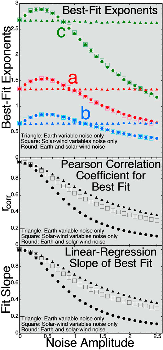
FIGURE 2. For a driver function of the form d = v₁^av₂^bv₃^c for three independent solar-wind variables v₁, v₂, and v₃, the exponents (A–C) are solved for as a function of time via an evolutionary algorithm that maximizes the Pearson linear correlation between d and e.

In the bottom panel of Figure 2 the slopes of linear-regression fits to the e values as functions of the best-fit d values are plotted as functions of the noise amplitude. (Both d and e are standardized here, with mean values of 0 and standard deviations of 1.) The slope values in the bottom panel track the correlation coefficients in the middle panel, commensurate with the regression-dilution-bias effect. I.e., for the linear best fit of e by v₁^av₂^bv₃^c, the coefficient in front of v₁^av₂^bv₃^c decreases with increasing noise.

Note that if there is vertical-only noise on the Earth measure (geomagnetic index) e but not in the solar wind, the coefficients obtained would not change with noise. However, the correlation r_corr decreases with noise (middle panel of Figure 2) and the regression dilution bias still occurs with the linear-regression slopes decreasing with noise amplitude (bottom panel of Figure 2) interpreted as lessened Earth reaction for an increased driver strength.

As a preview of future work, adding noise to the solar-wind variables in real data [i.e., OMNI2, King and Papitashvili (2005)] indeed changes the functional form of the best-fit solar-wind driver. Fits of the form v_sw^aB_sw^bsin^c (θ_clock/2) to various time-lagged geomagnetic indices (AE, AL, AU, Kp, Hp60, PCI) find that adding noise to any one of the three solar-wind variables changes the best-fit values of all three exponents a, b, and c. Depending on the geomagnetic index that is being fit, the best-fit values of a, b, or c can either decrease with added noise or increase with added noise. In agreement with the triangle points in the top panel of Figure 2, adding noise only to the geomagnetic index does not change the best-fit values of a, b, or c in a real data set. Real solar-wind data will be explored in a future report.

Summary

The functional form obtained for the best fit solar-wind driver d depends on (at least) two things. It is a function of how the driving works. It is also a function of noise in the measurements. If our goal is to use real solar-wind/magnetosphere data to uncover or to confirm the formula that tells us the physics of the driving, we have trouble because of there always being noise in the data. One source of error in the solar-wind and magnetosphere data is the fact that the solar wind that hits an upstream monitor is not the same solar wind that hits the earth: this error has been expounded upon (Borovsky, 2018; Borovsky, 2020b; Walsh et al., 2019; Burkholder et al., 2020). Another source of error is that geomagnetic indices are only indirect measures of the reaction of the earth to the solar wind. A future research effort might involve 1) obtaining a best-fit driver formula from the real data, 2) assessing the amplitude and properties of the noise in the real data, and 3) attempting to correct the formula for the effects of the noise.

Data Availability Statement

The original contributions presented in the study are included in the article/Supplementary Material, further inquiries can be directed to the corresponding author.

Author Contributions

The author confirms being the sole contributor of this work and has approved it for publication.

Funding

JB was supported by the NSF GEM Program via grant AGS-2027569, by the NASA HERMES Interdisciplinary Science Program via grant 80NSSC21K1406, and by the NASA Heliophysics Mission Concept Study Program via award 80NSSC22K0113.

Conflict of Interest

The author declares that the research was conducted in the absence of any commercial or financial relationships that could be construed as a potential conflict of interest.

Publisher’s Note

All claims expressed in this article are solely those of the authors and do not necessarily represent those of their affiliated organizations, or those of the publisher, the editors and the reviewers. Any product that may be evaluated in this article, or claim that may be made by its manufacturer, is not guaranteed or endorsed by the publisher.

Acknowledgments

The author wishes to thank Gian Luca Delzanno for helpful conversations.

References

Baker, D. N. (1986). Statistical Analyses in the Study of Solar Wind-Magnetosphere Coupling. in Solar Wind-Magnetosphere Coupling, Y. Kamide, and J. A. Slavin (eds.), p. 17, 38. Terra Scientific, Tokyo. doi:10.1007/978-94-009-4722-1_2
Balikhin, M. A., Boynton, R. J., Billings, S. A., Gadalin, M., Ganushkina, N., Coca, D., et al. (2010). Data Based Quest for Solar Wind-Magnetosphere Coupling Function. Geophys. Res. Lett. 37, L24107. doi:10.1029/2010gl045733
Bock, R. D., and Petersen, A. C. (1975). A Multivariate Correction for Attenuation. Biometrika 62, 673–678. doi:10.1093/biomet/62.3.673
Borovsky, J. E. (2020a). A Survey of Geomagnetic and Plasma Time Lags in the Solar-Wind-Driven Magnetosphere of Earth. J. Atmos. Solar-Terrestrial Phys. 208, 105376. doi:10.1016/j.jastp.2020.105376
Borovsky, J. E. (2014). Canonical Correlation Analysis of the Combined Solar Wind and Geomagnetic index Data Sets. J. Geophys. Res. Space Phys. 119, 5364–5381. doi:10.1002/2013ja019607
Borovsky, J. E., and Denton, M. H. (2018). Exploration of a Composite index to Describe Magnetospheric Activity: Reduction of the Magnetospheric State Vector to a Single Scalar. J. Geophys. Res. Space Phys. 123, 7384–7412. doi:10.1029/2018ja025430
Borovsky, J. E. (2021). Is Our Understanding of Solar-Wind/Magnetosphere Coupling Satisfactory? Front. Astron. Space Sci. 8, 634073. doi:10.3389/fspas.2021.634073
Borovsky, J. E. (2013). Physical Improvements to the Solar Wind Reconnection Control Function for the Earth's Magnetosphere. J. Geophys. Res. Space Phys. 118, 2113–2121. doi:10.1002/jgra.50110
Borovsky, J. E. (2018). The Spatial Structure of the Oncoming Solar Wind at Earth and the Shortcomings of a Solar-Wind Monitor at L1. J. Atmos. Solar-Terrestrial Phys. 177, 2–11. doi:10.1016/j.jastp.2017.03.014
Borovsky, J. E., Thomsen, M. F., and Elphic, R. C. (1998). The Driving of the Plasma Sheet by the Solar Wind. J. Geophys. Res. 103, 17617–17639. doi:10.1029/97ja02986
Borovsky, J. E. (2017). Time-integral Correlations of Multiple Variables with the Relativistic-Electron Flux at Geosynchronous Orbit: The strong Roles of the Substorm-Injected Electrons and the Ion Plasma Sheet. J. Geophys. Res. 122, 11961. doi:10.1002/2017ja024476
Borovsky, J. E. (2020b). What Magnetospheric and Ionospheric Researchers Should Know about the Solar Wind. J. Atmos. Solar-Terrestrial Phys. 204, 105271. doi:10.1016/j.jastp.2020.105271
Burkholder, B. L., Nykyri, K., and Ma, X. (2020). A Multispacecraft Solar Wind Monitor. J. Geophys. Res. 125, e2020JA027978. doi:10.1029/2020ja027978
Golub, G. H., and Van Loan, C. F. (1980). An Analysis of the Total Least Squares Problem. SIAM J. Numer. Anal. 17, 883–893. doi:10.1137/0717073
Hutcheon, J. A., Chiolero, A., and Hanley, J. A. (2010). Random Measurement Error and Regression Dilution Bias. BMJ 340, c2289–1406. doi:10.1136/bmj.c2289
King, J. H., and Papitashvili, N. E. (2005). Solar Wind Spatial Scales in and Comparisons of Hourly Wind and ACE Plasma and Magnetic Field Data. J. Geophys. Res. 110, 2104. doi:10.1029/2004ja010649
Liu, K. (1988). Measurement Error and its Impact on Partial Correlation and Multiple Linear Regression Analyses1. Am. J. Epidemiol. 127, 864–874. doi:10.1093/oxfordjournals.aje.a114870
McPherron, R. L., Hsu, T.-S., and Chu, X. (2015). An Optimum Solar Wind Coupling Function for theALindex. J. Geophys. Res. Space Phys. 120, 2494–2515. doi:10.1002/2014ja020619
Newell, P. T., Sotirelis, T., Liou, K., Meng, C.-I., and Rich, F. J. (2007). A Nearly Universal Solar Wind-Magnetosphere Coupling Function Inferred from 10 Magnetospheric State Variables. J. Geophys. Res. 112, A01206. doi:10.1029/2006ja012015
Riggs, D. S., Guarnieri, J. A., and Addelman, S. (1978). Fitting Straight Lines when Both Variables Are Subject to Error. Life Sci. 22, 1305–1360. doi:10.1016/0024-3205(78)90098-x
Smith, R. J. (2009). Use and Misuse of the Reduced Major axis for Line-Fitting. Am. J. Phys. Anthropol. 140, 476–486. doi:10.1002/ajpa.21090
Spearman, C. (1904). The Proof and Measurement of Association between Two Things. Am. J. Psychol. 15, 72. doi:10.2307/1412159
Walsh, B. M., Bhakyapaibul, T., and Zou, Y. (2019). Quantifying the Uncertainty of Using Solar Wind Measurements for Geospace Inputs. J. Geophys. Res. Space Phys. 124, 3291–3302. doi:10.1029/2019ja026507
Keywords: magnetosphere, solar wind, geomagnetic activity, geomagnetic indices, solar wind magnetosphere coupling, space weather
Citation: Borovsky JE (2022) Noise, Regression Dilution Bias, and Solar-Wind/Magnetosphere Coupling Studies. Front. Astron. Space Sci. 9:867282. doi: 10.3389/fspas.2022.867282
Received: 31 January 2022; Accepted: 21 February 2022;
Published: 04 March 2022.
Edited by:
David Ruffolo, Mahidol University, ThailandReviewed by:
Robert McPherron, Los Angeles County, California, United StatesZhenguang Huang, University of Michigan, United States
Copyright © 2022 Borovsky. This is an open-access article distributed under the terms of the Creative Commons Attribution License (CC BY). The use, distribution or reproduction in other forums is permitted, provided the original author(s) and the copyright owner(s) are credited and that the original publication in this journal is cited, in accordance with accepted academic practice. No use, distribution or reproduction is permitted which does not comply with these terms.
*Correspondence: Joseph E. Borovsky, jborovsky@spacescience.org