 Christopher P. Konrad1*
 Noah M. Schmadel2
 Judson W. Harvey2Gregory E. Schwarz2Jesus Gomez-Velez3Elizabeth W. Boyer4
 Durelle Scott5
- 1US Geological Survey, Tacoma, WA, United States
- 2US Geological Survey, Reston, VA, United States
- 3Department of Civil and Environmental Engineering, Vanderbilt University, Nashville, TN, United States
- 4Department of Ecosystem Science and Management, Pennsylvania State University, University Park, PA, United States
- 5Department of Biological Systems Engineering, Virginia Tech, Charlottesville, VA, United States
Retention, processing, and transport of solutes and particulates in stream corridors are influenced by the travel time of streamflow through stream channels, which varies dynamically with discharge. The effects of streamflow variability across sites and over time cannot be addressed by time-averaged models if parameters are based solely on the characteristics of mean streamflow. We develop methods to account for the effects of streamflow variability on travel time and compare our estimates to flow-weighted (“effective”) travel time at 100 streams in the southeastern United States. Velocity time series were generated for each stream from multiple-year (median 15.5 years), high-frequency (15 min interval) records of instantaneous streamflow and field measurements of velocity and inverted to produce time series of specific travel time [T/L]. The effective travel times for streams are 60–90% of the specific travel time of mean streamflow because a large fraction of the total streamflow volume is discharged during higher flows with higher velocities. We find that adjusting the specific travel time of mean streamflow at a site by a factor of 0.81 generally accounts for the effect of a skewed streamflow distribution, but at-site estimates of the coefficient of variation of streamflow are necessary to resolve differences in streamflow variability between streams or changes in variability over time. For example, the effective travel time of urban streams is less than the effective travel of forested streams in the southeastern United States as a result of increased streamflow variability in urban streams. Effective travel time accounts for both the variation in velocity with streamflow and the large fraction of streamflow discharged during high flows in most streams and provides time-averaged models with limited capability to account for effects of streamflow variability that otherwise they lack. This capability is needed for continental-scale modeling where streamflow variability is not uniform because of heterogeneous surficial geology, hydro-climatology, and vegetation and for applications where streamflow variability is not stationary as a response to climate change or hydrologic alteration.
Introduction
The velocity of streamflow has two fundamental but distinct roles on the processing of solutes and particulates in river corridors: it determines the rate of downstream advective transport of materials in a channel and it affects the “turnover length” of streamflow, which is the distance that streamflow must travel for complete exchange with water in transient storage zones in river corridors (e.g., hyporheic sediments, in-channel alcoves, off-channel sloughs, and floodplains) (Newbold et al., 1983; Meyer and Edwards, 1990; Mulholland et al., 1990; Stream Solute Workshop, 1990; Czuba and Foufoula-Georgiou, 2014; Harvey, 2016). The ratio of downstream advective transport to in-channel processing (e.g., settling velocity of particulates or uptake velocity of nutrients) limits the efficiency of in-channel retention of fine sediment in river channels (Konrad, 2009), filtration of organic particulates by invertebrates (Wallace et al., 1977), and nutrient uptake by photosynthetic organisms (Hall et al., 2002). Turnover lengths indicate hydrologic connectivity of streamflow (fraction exchanged) with hyporheic and other storage zones and its contact time with reactive sediments (Hein et al., 2004; Schmadel et al., 2016; Harvey et al., 2019; Findlay, 1995). Given these roles, streamflow velocity or, inversely, travel time is a lynch pin for accurate accounting of material processing and loads through river networks.
Large-scale synoptic investigations (Konrad and Gellis, 2018), remotely-acquired data (Konrad et al., 2008) and spatially-distributed models (Czuba et al., 2018) can address spatial variability in streamflow velocity, but high-frequency measurements and dynamic models are needed to account explicitly for the temporal variability of travel time forced by streamflow and its resulting effects on biophysical processing (Konrad, 2009; Botter et al., 2010; Basu et al., 2011; Ye et al., 2012). It is more often the case that time-averaged models of material transport and reactivity are applied to river networks (Boyer et al., 2006; Mulholland et al., 2008; Alexander et al., 2009; Helton et al., 2011; Czuba and Foufoula-Georgiou, 2014; Gomez-Velez et al., 2015). The temporal distributions of streamflow velocity and travel time remain a critical gap for river basin and larger scale biogeochemical modeling over seasonal and longer timescales (Wollheim et al., 2006; Bergstrom et al., 2016; Raymond et al., 2016). Since streamflow cannot be presumed to be steady over these time scales, effective values of velocity, and travel time are used in time-averaged models (Wolman and Miller, 1960; Doyle, 2005; Basso et al., 2015; Harvey and Gooseff, 2015). Application of such models to assess impacts of climate, land use, or water management in river corridors, however, requires adjustments to the effective values of velocity or travel time to account for changes in temporal variability of streamflow.
Time-averaged biogeochemical models of river networks typically use the velocity, travel time, or hydraulic load (product of velocity and depth divided by reach length) for mean streamflow (Behrendt and Opitz, 1999; Wollheim et al., 2006; Alexander et al., 2009; Helton et al., 2011). Mean streamflow, however, does not represent the variability of streamflow, which ranges across streams because of spatial heterogeneity in geology, soils, climate, watershed size, drainage density, and land cover (Carlston, 1963; Thomas and Benson, 1970; Poff and Ward, 1989; Dettinger and Diaz, 2000; Konrad et al., 2005; Pagano and Garen, 2005; Poff et al., 2007; Jiménez Cisneros et al., 2014; Basso et al., 2015). Without a way to represent differences in streamflow variability in space or over time, time-averaged models have limited capability to account for the effects of basin scale, climate, and hydrologic alteration by land and water uses (Ensign and Doyle, 2006; Wollheim et al., 2006; Hall et al., 2009; Basu et al., 2011; Raymond et al., 2016).
Urban development in particular increases streamflow variability as a result of reduced storage of water in soil and land surface depressions and shorter, less resistant pathways for water to flow through drainage systems into channels. These changes result in more rapid runoff and greater flow peaks for a given storm (Leopold, 1968; Konrad and Booth, 2005). Despite efforts to manage urban stormwater, modification of streamflow regimes persists in urban areas (Paul and Meyer, 2001; Konrad et al., 2005; Chang, 2007; Smith et al., 2013). While structural changes in stream channels (e.g., lining the channel with concrete, removing emergent vegetation) reduces flow resistance and travel time, shorter travel times in urban streams can be expected simply as a result of the re-distribution of runoff from lower-flow to higher-flow periods.
Our objective is to develop a method for estimating the effective travel time in stream channels that accounts for streamflow variability at and across sites and can conveniently be applied in time-averaged modeling stream transport and reaction of processes with first-order kinetics. The method is generalized by using the variance and skew of a streamflow distribution for the estimate without prejudice to why streamflow has a particular skew and variance. Thus, it is transferrable to infer effects on processing and retention for any factor that is known to influence the moments of a streamflow distribution. Potential applications extend to the evaluation of retention and processing of sediment and nutrients (1) at regional-scales because of heterogeneity in geology and hydro-climatology, (2) across large river basins because of downstream reduction in streamflow variability, and (3) in the context of climate and land use changes that affect streamflow variability. We demonstrate how differences in travel time at decadal time scales can be inferred from differences in streamflow distributions as a result of urban development in the southeastern United States.
Methods and Materials
Effective Travel Time for First-Order Reaction Processes
For in-stream processes involving first-order kinetics of transformation or retention (e.g., nutrient uptake that is a constant fraction of nutrient concentration), the effective travel time of water through a reach, Tref[T], can be derived by equating the mass flux calculated from a time-averaged model to the instantaneous mass flux integrated over time,
where k is the reaction rate constant, L is reach length, is mean concentration of the constituent of interest, is mean discharge, T is the total time for the period for interest, Ct is concentration at time t, Qt is discharge at time t, and ut is velocity at time t. By simplifying Equation (1), the effective travel time reduces to the flow- and concentration-weighted, mean travel time,
We limit the analysis to cases where temporal variation in streamflow is much greater than the variation in first-order reaction rates, k is constant, and variation in concentration using the approximations . These approximations allows Tref to be calculated simply as the flow-weighted mean travel time:
Based on Equation (3), flow-weighted travel times will generally be shorter than time-averaged travel time because velocity increases with streamflow. For cases where concentration and first-order reaction rates vary over time, the effective travel depends on the joint probability of travel time, concentration, and first-order reaction rate [see Doyle (2005) for an example of temporally variable streamflow and concentration]. When concentration increases with streamflow and first-order reaction rates decrease with concentration (e.g., a saturation effect), Equation (3) would provide a better estimate than the time-averaged travel time, but travel time would still be under-estimated.
Specific Travel Time
Calculation of effective travel time with Equation (3) requires time series of discharge and travel time. While discharge time series are available from gages and can be extrapolated over a reach without significant inflows and outflows or simulated using spatially-distributed hydrologic models, time series of travel time are only available at locations with velocity meters, hydraulic models, or where travel time has been measured over a range of streamflow (Hubbard et al., 1982; Bergstrom et al., 2016). For gaged streams with velocity data, a stage or discharge time series can be transformed into velocity time series (Jobson, 2000) and inverted to produce a time series of specific travel time, τt = 1/ut, [L/T] at the gage. The effective value (flow-weighted) of a distribution of specific travel times can be calculated from time series of discharge and velocity,
where ts represents an individual time step in each time series, TS is the total number of values in each time series, and τef is the effective value of specific travel time at the gage and time series used with units of [T/L].
Equation (4) is used to demonstrate the effects of streamflow variability on velocity and specific travel time. The velocity at a gage is not necessarily representative of velocity averaged over a reach but it is useful as an index of variation of the reach-averaged mean velocity over time (Hubbard et al., 1982). Specific travel time at a gage is likely to biased downward in comparison to the travel time for a longer reach because gage locations are typically selected in narrower sections that maintain measurable, downstream velocity even during low flows. The bias is likely to diminish as streamflow increases and flow becomes more uniform through the reach (Hubbard et al., 1982). As a result, the effect of streamflow variability on specific travel time at a gage indicated by this analysis is likely to be less than its effect on travel time at the reach-scale.
Overview of Analysis and Streams
The analysis has three principal steps: (1) synthesize τef distributions from multiple-year, instantaneous streamflow records and field-measured velocities for gaged streams spanning a range in streamflow variability; (2) apply and evaluate methods for estimating τef; and (3) compare τt distributions characteristic of urban and undeveloped streams. We selected 100 gaged streams in the southeastern United States (Figure 1) from six Level III Ecoregions: Piedmont (76 streams), Blue Ridge (12 streams), Valley and Ridge (8 streams), Southeastern Plains (2 streams), North Piedmont (1 stream), and Southwestern Appalachians (1 stream) (Journey et al., 2015). The streams span a range of drainage areas (7–1000 km2) and were selected to represent streamflow modification by reservoirs and land uses. Normal reservoir storage volume (US Army Corps of Engineers, 2010) in each stream basin divided by basin area ranged from 0 to more than 3 m (median value of 12 mm). Agricultural land cover ranged from 0 to 33% (median 6.5%) of stream basin area. Urban land cover ranged from <1 to 100% (median 22%). The values for each stream are available in Konrad (2020).
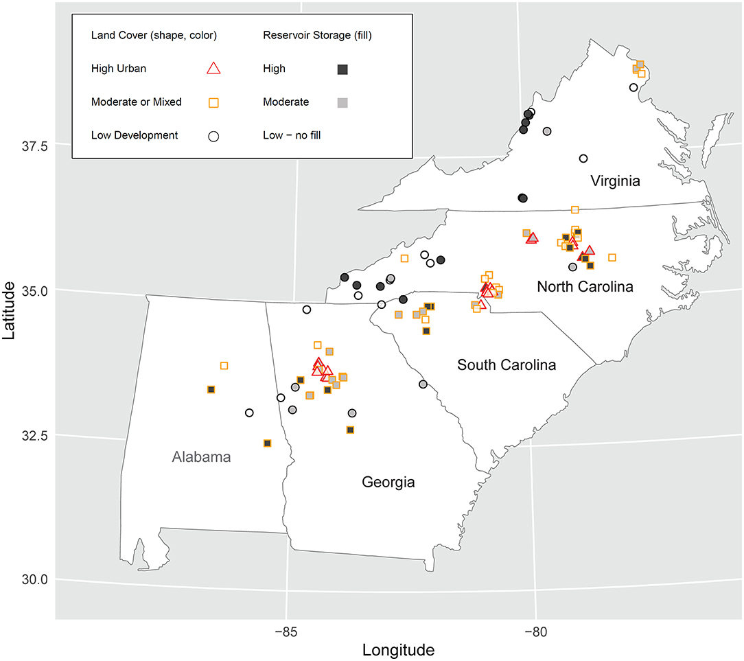
Figure 1. Location of streams in the southeastern US categorized by land cover and reservoir storage.
Stream size, land use, and streamflow regulation by reservoirs can all affect streamflow variability, so they are potential confounding factors when effects of urbanization on travel time. The coefficient of variation of streamflow distributions were examined in relation to drainage area, total agricultural and urban land cover in 2011 (Multi-Resolution Land Characteristics Consortium, 2019), and normal reservoir storage to identify domains where streamflow variability had little relation to each factor. These homoscedastic domains provided the basis for stratifying streams by size, land use, and regulation (Table 1).
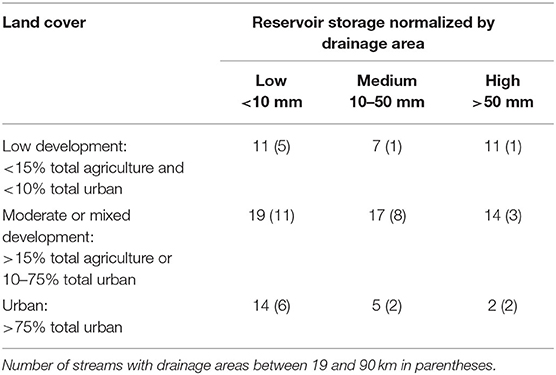
Table 1. Number of streams stratified by reservoir storage and land cover.
Although streams are distributed over the ranges of these factors, not all combinations are well-represented. Streams with drainage areas outside of the range from 19 to 90 km2, moderate development, mixed land use, or reservoirs providing more than 10 mm of storage over the stream's drainage area are excluded from the analysis of urbanization (step 3). Travel time is examined in streams where streamflow is regulated by reservoirs, but we do not test for effects because of differences in how reservoirs are operated among streams (e.g., power production, water supply, or flood control).
Generating Specific Travel Time Distributions From Streamflow Time Series and Discrete Velocity Measurements
Available instantaneous streamflow records with a 15 min interval from 1 October 2000 to 30 September 2017 were retrieved from the National Water Information System (USGS, 2019). The length of the records ranged from 4 to 17 years among the streams with a median of 15.5 years. Field measurements of velocity and streamflow were retrieved for 1 October 2010 to 30 September 2017 at each site (Rantz, 1982; USGS, 2019). The period for field measurements relating measured velocity to discharge was limited to the most recent 7 years of the streamflow records to increase the likelihood that measurements were made at approximately the same section in each stream so that at-site variation in velocity is primarily due to variation in discharge rather than the location of the measurement section.
The measurement of stream velocity during unsteady flow may include a significant component of localized, flood-wave driven celerity that affects channel storage rather than contributing to the downstream advection of water. We eliminated measurements made during periods of unsteady flow by converting instantaneous stage measured at the gage during each measurement into values of hydraulic mean depth for the cross-section and eliminating those measurements when hydraulic mean depth changed by more than 10% during the measurement (USGS, 2019). After eliminating measurements made during unsteady flow, streams had between 26 and 96 remaining measurements (median of 52 measurements per site) to define the relation between instantaneous streamflow and velocity.
Specific travel times, τt, [s/m] are synthesized for each stream by transforming instantaneous streamflow, Qt, into instantaneous velocity, ut, and inverting the velocities, τt = 1/ut. The transformation is based on linear regression of log of discrete streamflow measurements, Qm, and log of mean cross-section velocity, um, for the measurements in a stream, s, using the function lm in R (R Core Team, 2019) to minimize the sum of the squared errors εm for each site,
where β0,s is the intercept and β1,s is the slope for stream s assuming that the functional form is a power law, um = β01 (Rantz, 1982). The log of instantaneous travel time at time t, τt, is equal to the opposite of the velocity function applied to instantaneous streamflow,
Methods for Estimating Effective Travel Time
Application of biogeochemical models across river networks requires spatially distributed estimates of effective travel time. While Equations (4)–(6) can be used at locations with measured velocities and streamflow time-series, we develop and evaluate three alternative methods for estimating τef that could be applied more widely. Each method uses either a quantile or moment of a streamflow distribution, which could be calculated at gaged sites from streamflow records or, potentially, assigned to ungaged streams using a model. The overall purpose for the comparisons is to assess the viability of estimating τef from an index streamflow rather than computing it directly from the τt distribution. The evaluation of the estimates with respect to streamflow variability is significant for both selecting the best method but also understanding the bias of using any of these method in comparisons across streams or scenarios where streamflow variability neither uniform in space or constant over time.
Direct calculation of τef and all of the methods for estimating τef depend on a known relation between discharge and travel time, which will be a primary source of uncertainty in any application. Estimation of τef faces an additional issue of bias related to streamflow variability, which limits the utility of τef estimates in comparative analyses across streams (e.g., in relation to basin size, climate, or land use) or over time (e.g., in relation to changes in climate, land use, or water management). Errors in estimates of τef from each method are compared to the variance and higher moments of streamflow distributions to evaluate bias with streamflow variability.
The first method for estimating τef uses the specific travel time for a fixed quantile of a streamflow distribution. This method accounts for the effect of streamflow variability on travel time generalized across sites but depends on a relatively consistent effect across sites for unbiased estimation. The effective discharge, Qef, that has a specific travel time equal to τef is calculated by inverting Equation (6) and replacing τt with τef for each stream,
The quantiles representing Qef are compared to each of the first three linear (L-) moment ratios (Hosking and Wallis, 1997) of the observed streamflow distributions for the 100 streams:
where λi is the ith L-moment of the observed streamflow frequency distribution (Hosking, 2017). Systematic variation of the quantile for τef with one or more of the L-moment ratios would indicate potential bias when using fixed quantile of streamflow distributions to estimate τef among streams with differences in streamflow variability.
The second method for estimating τef would adjust the travel time of mean streamflow for a stream, , by a constant, τ* = τef: representing the ratio of effective travel time to the travel time of mean streamflow. The effective travel time, , at a site is estimated as
where is calculated by substituting for Qt in Equation (6) using the regression coefficients β0,s and β1,s from Equation (5). The median cross-site ratio of τef: is used for τ* in Equation (9).
We expect that τ* will decrease with streamflow variability, so the third estimation method would adjust τ* in Equation (9) based on a streamflow distribution's L-moment ratios. Our primary question is whether the LCV is adequate for adjusting τ* to account for the effects of streamflow variability on τef or higher-order moment ratios are necessary to prevent variability-biased estimation. The strength of the relation between the τ* and each of the first three empirical L-moment ratios (Equations 8a,b,c) is tested using Kendall rank correlation coefficients. Finally, the L-moment ratio with the strongest correlation across sites is used to derive a power function for estimating τ*:
fit for the selected L-moment ratio, , using non-linear least squares regression (R Core Team, 2019).
Effects of Urban Runoff on Travel Time
The effects of streamflow variability on travel time are demonstrated for the case of urban land development, which increases streamflow variability as a result of the re-distribution of water from flow paths slowed by interactions with hillslope storage (depression and soil) to overland flow and low-resistance flow through engineered drainage systems. Streamflow and specific travel time distributions for streams draining urbanized watersheds are compared to those distributions for streams draining watersheds with low development (Table 1).
The Wilcoxon rank-sum test is applied to identify significant differences in travel time, velocity, and effective discharge between low-development and urban streams with low reservoir storage. L-moment ratios were not correlated with drainage area for low development streams with drainage areas between 19 and 90 km2, so the analysis of urbanization is limited to streams in this range of drainage areas to control for effects from basin scale.
Generalized effects of urban hydrologic alteration are synthesized by comparing travel time distributions generated from two theoretical streamflow distributions: one characteristic of a low-development stream and the other characteristic of an urban stream. There is no standard theoretical distribution used to represent instantaneous streamflow (Schaefli et al., 2013; Blum et al., 2017) so Generalized Extreme Value (GEV), 4-parameter Kappa, and Generalized Logistic distributions are evaluated as potential functional forms for the theoretical distributions. Each of the three theoretical distribution is fit to each site using the method of L-moments (Hosking and Wallis, 1997), such that the L-moments for the theoretical distribution matches the empirical L-moments of the instantaneous streamflow distributions to the extent possible.
The fit of each theoretical distribution is evaluated at each site using the one-sample Kolmogorov-Smirnov test (R Core Team, 2019) and a two-sided probability, p < 0.05 that the sample was drawn from the distribution. The theoretical distribution that is acceptable at the largest number of sites is selected as the functional form for the probability distributions of instantaneous streamflow. To verify that the theoretical streamflow distribution reproduces τef at a site, cumulative distributions of specific travel time and τef are calculated from Equations (4) and (6) using the theoretical streamflow distributions.
The characteristic parameters for a low-development stream and an urban stream are assigned using the median values of L-moment ratios for the five low-development streams and six urban streams with drainage areas between 19 and 90 km2. The parameters of the velocity function are not correlated across sites (Figure 2), so the cross-site median values of all 11 streams (β0 = 0.27, β1 = 0.48) are used to calculate the specific travel times (Equation 6) characteristic of both the low-development stream and the urban stream. Using the same parameters in Equation (6) prevents differences related to channel hydraulics from affecting the travel time calculations.
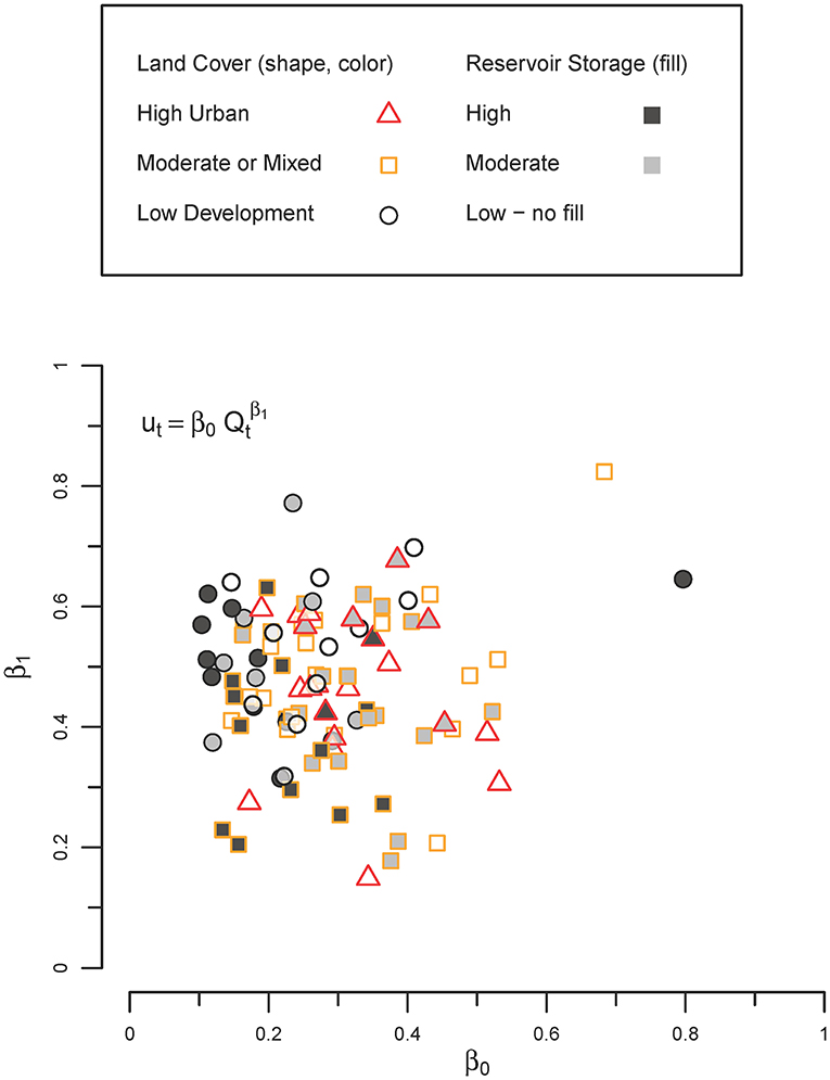
Figure 2. Velocity function (Equation 5) parameters for 100 streams in the southeastern US.
Results
Effective Travel Times in Relation to Streamflow Distributions
The effective (flow-weighted mean) value of specific travel time varies among the 100 streams from τef = 0.88–8.3 s/m (median of 3.1 s/m, Table 2). For streams with both low development and reservoir storage (n = 11, Table 1), τef was negatively correlated with drainage area (Kendall rank correlation coefficient of −0.6, p < 0.01 that correlation coefficient is zero) indicating that smaller streams generally have longer travel times when compared to larger streams. The relation generally holds regardless of land use and regulation by reservoirs, but τef still ranges widely among streams with approximately the same drainage area (Figure 3A).
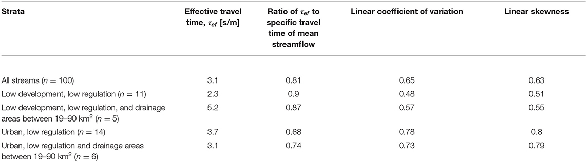
Table 2. Cross-site median values of travel time and instantaneous streamflow distribution statistics for five strata of streams.
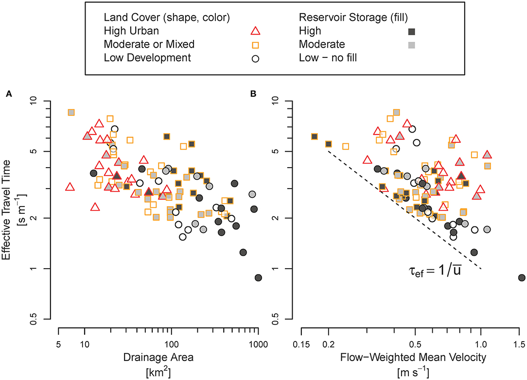
Figure 3. Effective (flow-weighted mean) value of specific travel time for 100 streams in the southeastern US in relation to: (A) the drainage area of their watersheds; and (B) flow-weighted mean velocity, with a dashed line indicating where travel time would be equal to the inverse of flow-weighted mean velocity.
Overall, τef is poorly correlated with flow-weighted mean velocity (Kendall rank correlation of 0.1, p = 0.13 that correlation coefficient is zero) and, without exception, τef is longer than the inverse of flow-weighted mean velocity in all streams (Figure 3B). The inverse relation between instantaneous velocity and specific travel time does not hold for their flow-weighted mean values because of the skew of the velocity distribution with respect to streamflow is inverted when its transformed into travel times using Equation (6): instantaneous velocities have larger deviations from their flow-weighted mean during high flows than low flows while, inversely, instantaneous travel times have larger absolute deviations from τef during low flows than high flows. Flow-weighted mean velocity is influenced by both the velocity magnitude and volume of high flows. In contrast, τef is sensitive to the long travel times during low flows despite their lower volumetric weighting. As a result, τef cannot be estimated simply by inverting the flow-weighted mean velocity of a stream.
The quantile of a streamflow distribution that has a specific travel time equal to τef is not consistent across sites: it ranges from the 0.52 (about median streamflow) to 0.97 (a relatively infrequent high flows) across streams (Figure 4). Across all sites, the quantile for τef is <0.7 in only three streams–all with more than 50 mm of reservoir storage. The streamflow quantile corresponding to τef is strongly correlated with both the linear skew (Figure 4A) and linear kurtosis of streamflow distributions (Kendall rank correlation coefficient >0.7, p < 0.001 that coefficient is zero for either). Variation in velocity with streamflow, which is indicated by the exponent, β1, for the velocity function (Equation 6), does not account for much of the cross-site variation in the quantile of streamflow that has a specific travel time equal to τef (Figure 4B).
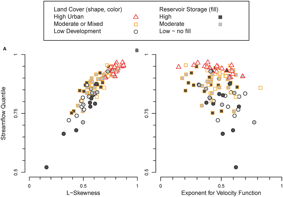
Figure 4. The streamflow quantile with a specific travel time equal to the effective travel time in relation to (A) linear (L-) skewness of the streamflow distribution and (B) the exponent for the velocity-discharge function (Equation 5).
Effects of Hydrologic Modification on Travel Time
The relation between streamflow variability and effective travel time leads to divergent responses of effective travel time to urbanization compared to reservoirs. Increased runoff from urbanized areas leads to higher variance and skew of instantaneous streamflow distributions (Table 2). As a result, a greater relative volume of streamflow has short travel times in urban streams compared to low-development streams (Wilcoxon rank sum test one-sided p < 0.001 that quantiles for τef are equal for urban and low-development streams, Table 2). Channel modifications associated with urbanization (e.g., lining, straightening, removing obstruction, disconnection from overbank areas) typically increase the velocity of urban streams, but the re-distribution of runoff in response to urbanization (Figure 4A) rather than changes in channel hydraulics that affect either flow-weighted mean velocity (Figure 3B) or the variation of velocity with streamflow (Figure 4B) is likely the primary control on changes in the travel time for urban streams. In contrast, a reservoir that stores water during periods of high flow and releases it at lower flows reduces the skew of a streamflow distribution, resulting in τef that represents the specific travel time of a lower quantile of streamflow (Figure 4A). Not all reservoirs are operated in ways that reduce the skew of a streamflow distribution, so their effect on travel time is less consistent that the effect of urbanization (Figure 4A).
Comparison of Methods for Estimating τef
Positively skewed, at-site streamflow distributions generally result in effective travel times that are less than the specific travel times of either median or mean streamflow (Figures 4, 5). Using the specific travel time of the 0.89 quantile (the cross-site median value) of a streamflow distribution to estimate τef at a site, the first estimation method had a RMSE of 1.2 s/m (Table 3). The second estimation method (Equation 9) adjusts the specific travel time of mean streamflow, , (Figure 5) by the cross-site median ratio τef:, τ* = 0.81 and had a RMSE of 0.56 s/m.
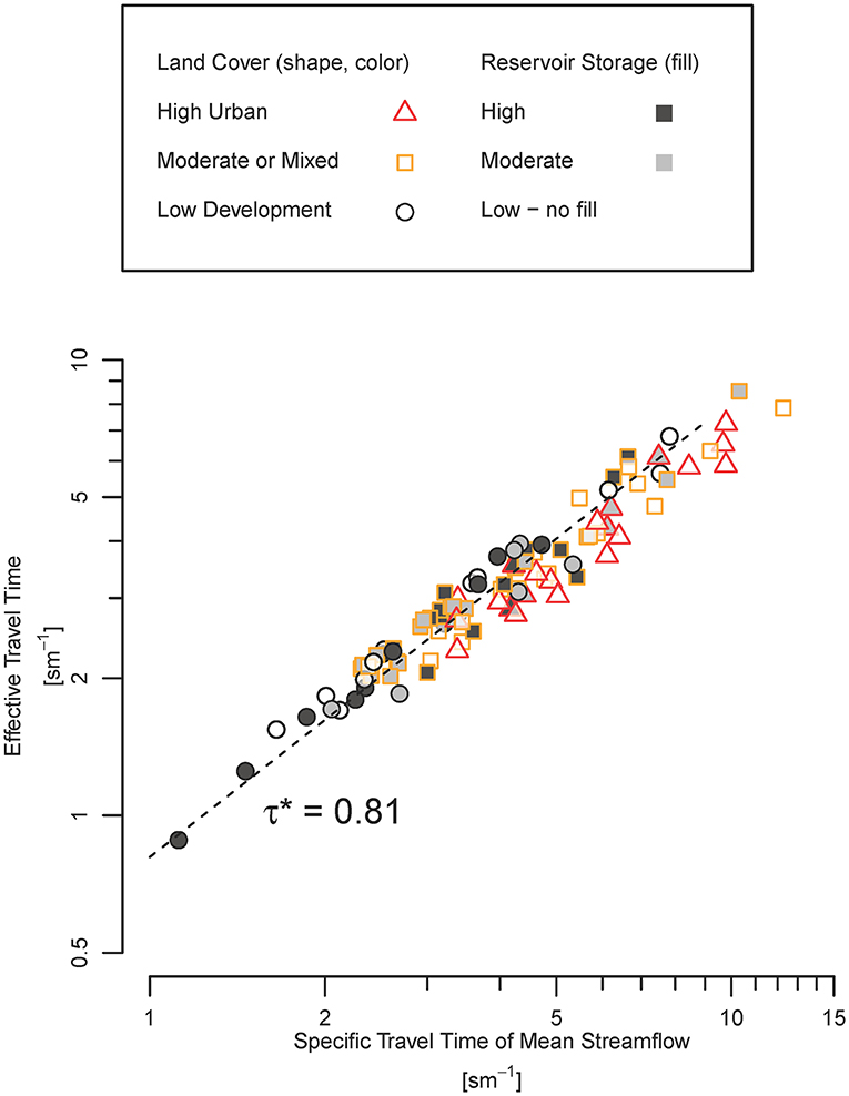
Figure 5. Specific travel time of mean streamflow and effective travel time for 100 streams in the southeastern United States. The cross-site median ratio is τ* = 0.81.
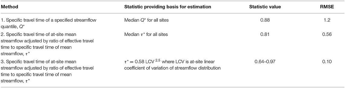
Table 3. Summary of methods for estimating effective travel time.
The ratio indicates that τef generally is about 20% shorter than and is needed to address this general bias from using mean streamflow to estimate τef. Mean streamflow provides a better basis for estimating τef (second method) than a fixed quantile (first method) because the mean value of a streamflow distribution is leveraged by the magnitude of high flows while a quantile reflects that time that streamflow is less than or equal a given magnitude without regard to how streamflow above or below the quantile is distributed.
The ratio of effective travel time in a stream to the specific travel time of its mean streamflow decreases as the variability of the stream's streamflow distribution increases (the inverse relation between τ* and LCV in Figure 6). Thus, at-site estimation of τef using the specific travel time of mean streamflow has increasing bias with streamflow variability. Urban streams, in particular, have highly variable and skewed streamflow distributions (Figures 4A, 6, respectively) and, as a consequence, effective travel times are much shorter that the travel time of mean streamflow (median τ* = 0.69 for urban streams, Table 2) compared low-development streams (median τ* = 0.9, p < 0.001 that τ* of urban streams are equal to or greater than τ* of low-development/low-regulation streams, one-sided Wilcoxon test).
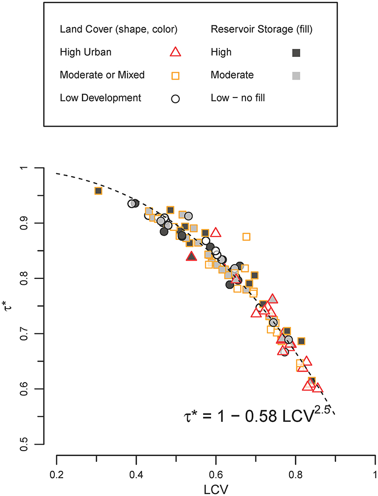
Figure 6. Ratio of flow-weighted travel time to travel time of mean streamflow, τ*, in relation to linear coefficient of variation, LCV. Dashed line is τ* = 1–0.58 LCV2.5.
The third estimation method uses stream-specific values of τ* based on the variability of the streamflow distribution for a stream to adjust the travel time of mean streamflow. Stream-specific values of τ* vary inversely with the LCV of streamflow distributions (Figure 6) but can be estimated from LCV by the power function:
Estimates of τef from Equation (9) with τ* calculated for each site from Equation (11) had a RMSE 0.1 s/m (Table 3). The bias of estimates from the third method is substantially lower than from the other two methods (Table 2) indicating how the increasing variance of a streamflow distribution scaled by its mean value reduces effective travel time τef.
Effect of Urbanization on Specific Travel Time
Streamflow distributions with variability characteristic of a low-development stream and an urban stream, respectively, were generated from a generalized extreme value (GEV). The GEV distribution provides a better approximation of instantaneous streamflow distributions than either the Kappa or Generalized Logistic distributions for all 100 streams but still could be rejected at 31 of them (two-sided p < 0.05 K-S test). Nonetheless, τef calculated from Equation (6) using a GEV distribution fit to each stream to generate Qt provides robust at-site estimates that closely matched τef calculated from Equation (6) using observed streamflow values for Qt (RMSE = 0.057 s/m; Figure 7).
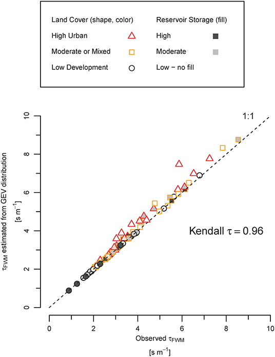
Figure 7. Flow-weighted mean travel time (τef) calculated from the observed streamflow distribution and a GEV distribution fit to each stream using L-moments.
The median values of GEV-distribution parameters for small, urban streams (n = 6) are distinct from those for small low-development streams (n = 5) and generally indicate the urban streams have higher variance and skew (Figure 8, Table 4). As a result, the travel time distribution for the characteristic urban stream generally shifts toward larger volumes of water with shorter travel times (Figure 9). The characteristic urban stream has an 19% increase in the volume of streamflow with relative short travel times (<1 s/m) and a 21% decrease in streamflow with travel times between 2 and 4 s/m compared to the characteristic low-development stream (Figure 9A). The re-distribution of streamflow to higher flows in the urban stream generally increases the volume of urban streamflow with travel times < ~4 s/m (Figure 9B). The urban stream has slightly more streamflow with travel times >8 s/m (extremely low flow) than the low-development stream, but this represents a small portion (~2.5%) of total streamflow.
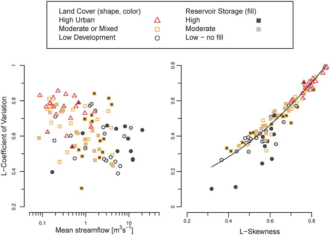
Figure 8. Linear moments for the instantaneous streamflow distributions of 100 streams in the southeastern United States. Line shows the relation between L-Skewness and L-Coefficient of Varation for generalized extreme value distributions.
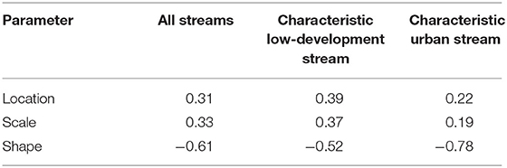
Table 4. Parameters used in the Generalized Extreme Value (GEV) distributions for characteristics streamflow distributions based on the median values for all streams, low-development streams with low reservoir storage and drainage areas between 19 and 90 km2 (characteristic low-development stream), and urban streams with low reservoir storage and drainage areas between 19 and 90 km2 (characteristic urban streams).
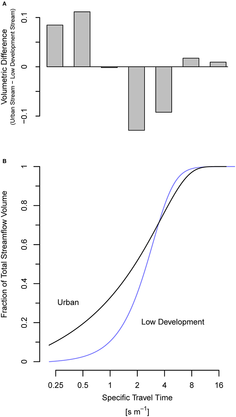
Figure 9. Travel-time distributions for characteristic a low-development and urban stream reach with (A) the marginal difference between the urban and low-development streams in standardized volume [fraction of total] for seven bins of travel time and (B) the cumulative distribution of streamflow by volume for the range of travel times from 0.2 to 20 s/m. Fraction of streamflow volume with travel times <0.2 s/m is 0% for the low-development stream and 8% for the urban stream.
Discussion
The specific travel time of mean streamflow is longer than the effective travel time of streamflow, τef, over annual and longer time scales because streamflow distributions are positively skewed (Blum et al., 2017) with most of the total volume discharge during higher flows with shorter travel times (Figure 5B). The difference between τef and the travel time of mean streamflow generally is about 20% (or equivalently τ* ≈ 0.8). Streams with higher streamflow variability have a larger relative volume of high flows with short travel times and, thus, shorter effective travel times (Figure 6).
Flow-weighting of travel time in Equation (4) provides a physically based value of τef, for modeling transport and processing at annual and longer time scales. Using τef, rather than τQmean in the empirical power-law expression for nitrogen removal proposed by Seitzinger et al. (2002), we would expect ~10% less nitrogen removal over a kilometer of channel. This is a significant difference in the mass of nitrogen retained, and it can have important cumulative effects for predictions at the river basin scale. While physically-based parameters have epistemic value for how processes scale over space and time and offer the promise of model parameterization from direct measurement, they do not necessarily improve model performance at calibration sites because of equifinality: parameters can compensate for each other's value resulting in comparable model performance for different parameter sets (Beven and Smith, 2015). Indeed, calibration of rate coefficients can offset the effect a particular travel time in a time-averaged biogeochemical model. Using the travel time of mean streamflow, however, will produce lower uptake velocities and deposition rates than models using τef.
The primary reason for using effective travel times in time-average models is to increase the capability of such models to simulate the effects of streamflow variability. Simply using 80% of the travel time of mean streamflow (method 2), however, does not provide time-averaged models with capability to represent differences between streams as a result of streamflow variability. The third method we developed provides relatively accurate estimates of τef (Table 3) but the at-site mean and variance of a streamflow distribution must be known to apply it. Low prediction skill of current models for the variance of streamflow (Farmer et al., 2014; Basso et al., 2015) is a crux for broader application of this estimation method to ungaged streams, but systematic variation in the LCV with land use (Figure 8) indicates the possibility for model-based estimation in some situations.
Effective travel time does not account for the dependencies of constituent concentrations on streamflow or first-order reaction rates on constituent concentrations. In cases where the temporal variability of concentrations and reaction rates are comparable to the variability of travel time, the joint distribution of streamflow, travel time, concentration, and first-order reaction rate is necessary to calculate an accurate, time-average mass flux for the process of interest (Doyle, 2005). If all such data were available, using a dynamic model would probably be preferable to a time-average model. Given that time series of velocity can be derived more widely (at streamflow gages with field measurements of velocity) than time series of concentration and reaction rate for any solute or particulate, adjustment of travel times is a pragmatic and broadly applicable approach to improve the capability of time-average river network models to represent effects of streamflow variability on biogeochemical processing in river networks.
For urban streams, a large fraction of the total runoff from the catchment is discharged during high-flow periods when streamflow has higher velocities in comparison to lower-flow periods. Even where stormwater detention controls peak flow rates, it has limited effectiveness reducing the volume of runoff during large storms (Booth et al., 2002; Hood et al., 2007; Smith et al., 2013). The volumetric differences between our characteristic undeveloped and urban streams are small for low flows longer travel time (e.g., >4 s/m), so substantial differences in processing would not be expected during low flow except for uptake or reactions with low mass-transfer coefficients. Difference only emerges for high flows when a large fraction of streamflow has short travel times (e.g., <1 s/m) in urban stream (Figure 7).
The effect of urbanization on nitrogen retention during base flow conditions is equivocal. In the desert Southwest, Grimm et al. (2005) documented less retention (longer uptake lengths) of experimental NO3- additions in urban streams but a strong effect from discharge. Using an expanded set of 72 streams, Hall et al. (2009) found uptake lengths varied with specific discharge (streamflow divided by width) streamflow at the time of the experiment (“stream size”) but not land-use per se. Hall et al. (2009) recommended that hydrologic variability is critical for understanding differences in nitrogen retention at longer time scales. We propose streamflow variability is likely to reduce retention given the well-defined, inverse relation of effective travel time to streamflow variability (Figure 6), but verification would require high-flow experiments [e.g., Melis (2011)] and the integration of results for both low and high flows based on streamflow distributions.
Effects of streamflow variability on processing and retention in streams are important in the context of land use (Hall et al., 2009), variation between headwater streams and mainstem rivers (Gomez-Velez et al., 2015), and responses to climate change (Baron et al., 2013; Morse and Wollheim, 2014). Given the relation between effective travel time and variance of streamflow distributions (Figure 6), differences in travel time can be inferred broadly from the effects of drainage area (Figure 2) (Thomas and Benson, 1970; Dunne and Leopold, 1978), regional climate (Dettinger and Diaz, 2000), climate change (Pagano and Garen, 2005; Jiménez Cisneros et al., 2014), reservoirs (Figure 2) (Poff et al., 2007; Kroll et al., 2015), and engineered-drainage systems (King et al., 2015) on the variance of streamflow distributions. Globally, anthropogenic changes to streamflow continues to expand with more extensive drainage systems, river impoundments and diversions, and land cover conversion and changes in climate (Eng et al., 2013; Jiménez Cisneros et al., 2014; King et al., 2015; Kroll et al., 2015; Carlisle et al., 2019). As these factors affect streamflow variability, travel times in biogeochemical models need to be adjusted accordingly.
Conclusions
Streamflow variability forces dynamic processing and retention of materials in river networks. The effective (flow-weighted mean) travel time of streamflow generally is less than the travel time of mean streamflow over seasonal and longer time scales because a significant fraction of streamflow is discharged at high velocities during high flows in most streams. The effective travel time of streamflow is typically ~80% of the travel time of mean streamflow for 100 streams in the southeastern United States and increases with streamflow variability. Application of the travel time of mean streamflow introduces a systematic bias in modeling of processing and retention where streamflow variability is neither uniform across streams nor constant over time. This bias limits the capability of time-averaged river-networks models to resolve differences between streams or changes over time. Time-average models can gain the capability to represent effects of streamflow variability by adjusting the travel time of mean streamflow using the at-site coefficient of variation of streamflow. This approach provides a pragmatic way to connect our understanding of spatial patterns in streamflow variability and its response to climate and land use change to processing and retention of transported materials (e.g., sediment, nutrients, contaminants) in river networks.
Data Availability Statement
Publicly available datasets were analyzed in this study. This data can be found here: Instantaneous streamflow values and field measured velocity and streamflow are available from the US Geological Survey National Water Information System. Data derived in this investigation are available from US Geological Survey ScienceBase (https://doi.org/10.5066/P9665F6L).
Author Contributions
CK proposed the objective and approach for this research during a workshop lead by JH, JG-V, EB, and DS. NS, GS, JH, and CK designed the analysis for general validity and broad relevance. CK compiled data, implemented the analysis, and drafted the initial manuscript. All of the authors were involved in preparing the final manuscript.
Funding
This research was supported by the US Geological Survey as part of the Regional Stream Quality Assessment and the River Corridor Working Group at the John Wesley Power Center for Analysis and Synthesis.
Conflict of Interest
The authors declare that the research was conducted in the absence of any commercial or financial relationships that could be construed as a potential conflict of interest.
Any use of trade, firm, or product names is for descriptive purposes only and does not imply endorsement by the U.S. Government.
References
Alexander, R. B., Böhlke, J. K., Boyer, E. W., David, M. B., Harvey, J. W., Mulholland, P. J., et al. (2009). Dynamic modeling of nitrogen losses in river networks unravels the coupled effects of hydrological and biogeochemical processes. Biogeochemistry 93, 91–116. doi: 10.1007/s10533-008-9274-8
Baron, J. S., Hall, E. K., Nolan, B. T., Finlay, J. C., Bernhardt, E. S., Harrison, J. A., et al. (2013). The interactive effects of excess reactive nitrogen and climate change on aquatic ecosystems and water resources of the United States. Biogeochemistry 114, 71–92. doi: 10.1007/s10533-012-9788-y
Basso, S., Frascati, A., Marani, M., Schirmer, M., and Botter, G. (2015). Climatic and landscape controls on effective discharge. Geophys. Res. Lett. 42, 8441–8447. doi: 10.1002/2015GL066014
Basu, N. B., Rao, P. S. C., Thompson, S. E., Loukinova, N. V., Donner, S. D., Ye, S., et al. (2011). Spatiotemporal averaging of in-stream solute removal dynamics. Water Resour. Res. 47:W00J06. doi: 10.1029/2010WR010196
Behrendt, H., and Opitz, D. (1999). Retention of nutrients in river systems: dependence on specific runoff and hydraulic load. Hydrobiologia 410, 111–122. doi: 10.1023/A:1003735225869
Bergstrom, A., McGlynn, B., Mallard, J., and Covino, T. (2016). Watershed structural influences on the distributions of stream network water and solute travel times under baseflow conditions. Hydrol. Process. 30, 2671–2685. doi: 10.1002/hyp.10792
Beven, K., and Smith, P. (2015). Concepts of information content and likelihood in parameter calibration for hydrological simulation models. J. Hydrol. Eng. 20:A4014010. doi: 10.1061/(ASCE)HE.1943-5584.0000991
Blum, A. G., Archfield, S. A., and Vogel, R. M. (2017). On the probability distribution of daily streamflow in the United States. Hydrol. Earth Syst. Sci. 21, 3093–3103. doi: 10.5194/hess-21-3093-2017
Booth, D. B., Hartley, D., and Jackson, R. (2002). Forest cover, impervious-surface area, and the mitigation of stormwater impacts. J. Am. Water Resour. Assoc. 38, 835–845. doi: 10.1111/j.1752-1688.2002.tb01000.x
Botter, G., Basu, N. B., Zanardo, S., Rao, P. S. C., and Rinaldo, A. (2010). Stochastic modeling of nutrient losses in streams: interactions of climatic, hydrologic, and biogeochemical controls. Water Resour. Res. 46:W08509. doi: 10.1029/2009WR008758
Boyer, E. W., Alexander, R. B., Parton, W. J., Li, C. S., Butterbach-Bahl, K., Donner, S. D., et al. (2006). Modeling denitrification in terrestrial and aquatic ecosystems at regional scales. Ecol. Appl. 16, 2123–2142. doi: 10.1890/1051-0761(2006)016[2123:MDITAA]2.0.CO;2
Carlisle, D. M., Wolock, D. M., Konrad, C. P., McCabe, G. J., Eng, K., Grantham, T. E., et al. (2019). Flow Modification in the Nation's Streams and Rivers. Technical Report, U.S. Geological Survey Circular 1461, Reston, VA. doi: 10.3133/cir1461
Carlston, C. W. (1963). Drainage Density and Streamflow. Technical Report, U.S. Geological Survey Prof. Paper 422–C, Washington, DC. doi: 10.3133/pp422C
Chang, H. (2007). Comparative streamflow characteristics in urbanizing basins in the Portland Metropolitan Area, Oregon, USA. Hydrol. Process. 21, 211–222. doi: 10.1002/hyp.6233
Czuba, C. R., Czuba, J. A., Magirl, C. S., Gendaszek, A. S., and Konrad, C. P. (2018). Effect of river confinement on depth and spatial extent of bed disturbance affecting salmon redds. J. Ecohydraul. 3, 4–17. doi: 10.1080/24705357.2018.1457986
Czuba, J. A., and Foufoula-Georgiou, E. (2014). A network-based framework for identifying potential synchronizations and amplifications of sediment delivery in river basins. Water Resour. Res. 50, 3826–3851. doi: 10.1002/2013WR014227
Dettinger, M. D., and Diaz, H. F. (2000). Global characteristics of stream flow seasonality and variability. J. Hydrometeorol. 1, 289–310. doi: 10.1175/1525-7541(2000)001<0289:GCOSFS>2.0.CO;2
Doyle, M. W. (2005). Incorporating hydrologic variability into nutrient spiraling. J. Geophys. Res. 110:G01003. doi: 10.1029/2005JG000015
Dunne, T., and Leopold, L. B. (1978). Water in Environmental Planning. New York, NY: W.H. Freeman and Company. 818.
Eng, K., Carlisle, D. M., Wolock, D. M., and Falcone, J. A. (2013). Predicting the likelihood of altered streamflows at ungauged rivers across the conterminous United States. River Res. Appl. 29, 781–791. doi: 10.1002/rra.2565
Ensign, S. H., and Doyle, M. W. (2006). Nutrient spiraling in streams and river networks. J. Geophys. Res. 111:G04009. doi: 10.1029/2005JG000114
Farmer, W. H., Archfield, S. A., Over, T. M., Hay, L. E., LaFontaine, J. H., and Kiang, J. E. (2014). A Comparison of Methods to Predict Historical Daily Streamflow Time Series in the Southeastern United States. Technical Report, U.S. Geological Survey Scientific Investigations Report 2014–5231, Reston, VA. doi: 10.3133/sir20145231
Findlay, S. (1995). Importance of surface-subsurface exchange in stream ecosystems: The hyporheic zone. Limnol. Oceanogr. 40, 159—64. doi: 10.4319/lo.1995.40.1.0159
Gomez-Velez, J., Harvey, J., Cardenas, M., and Kiel, B. (2015). Denitrification in the Mississippi River network controlled by flow through river bedforms. Nature Geosci. 8, 941–945. doi: 10.1038/ngeo2567
Grimm, N. B., Sheibley, R. W., Crenshaw, C. L., Dahm, C. N., Roach, W. J., and Zeglin, L. H. (2005). N retention and transformation in urban streams. J. N. Am. Benthol. Soc. 24, 626–642. doi: 10.1899/04-027.1
Hall, R. O. Jr., Bernhardt, E. S., and Likens, G.E. (2002). Relating nutrient uptake with transient storage in forested mountain streams. Limnol. Oceanogr. 47, 255–265. doi: 10.4319/lo.2002.47.1.0255
Hall, R. O. Jr., Tank, J. L., Sobota, D. J., Mulholland, P. J., O'Brien, J. M., Dodds, W. K., et al. (2009). Nitrate removal in stream ecosystems measured by 15N addition experiments: total uptake. Limnol. Oceanogr. 54, 653–665. doi: 10.4319/lo.2009.54.3.0653
Harvey, J., Gomez-Velez, J., Schmadel, N., Scott, D., Boyer, E., Alexander, R., et al. (2019). How hydrologic connectivity regulates water quality in river corridors. J. Am. Water Resour. Assoc. 55, 369–381. doi: 10.1111/1752-1688.12691
Harvey, J., and Gooseff, M. (2015). River corridor science: hydrologic exchange and ecological consequences from bed forms to basins. Water Resour. Res. 51, 6893–6692. doi: 10.1002/2015WR017617
Harvey, J. W. (2016). “Hydrologic exchange flows and their ecological consequences in river corridor in stream ecosystems in a changing environment,” in Stream Ecosystems in a Changing Environment, eds J. B. Jones and E. M. Stanley (Amsterdam: Elsevier), 1–83. doi: 10.1016/B978-0-12-405890-3.00001-4
Hein, T., Baranyi, C., Reckendorfer, W., and Schiemer, F. (2004). The impact of surface water exchange on the nutrient and particle dynamics in side-arms along the River Danube, Austria. Sci. Total Environ. 328, 207–218. doi: 10.1016/j.scitotenv.2004.01.006
Helton, A. M., Poole, G. C., Meyer, J. L., Wollheim, W. M., Peterson, B. J., Mulholland, P. J., et al. (2011). Thinking outside the channel: modeling nitrogen cycling in networked river ecosystems. Front. Ecol. Environ. 9, 229–238. doi: 10.1890/080211
Hood, M. J., Clausen, J. C., and Warner, G. S. (2007). Comparison of stormwater lag times for low impact and traditional residential development. J. Am. Water Resour. Assoc. 43, 1036–1046. doi: 10.1111/j.1752-1688.2007.00085.x
Hosking, J., and Wallis, J. (1997). Regional Frequency Analysis: An Approach Based on L-Moments. Cambridge: Cambridge University Press. doi: 10.1017/CBO9780511529443
Hosking, J. R. M. (2017). L-Moments, R package lmom, Version 2.8, 2019-03-11. Available online at: https://cran.r-project.org (accessed May 20, 2020).
Hubbard, E. F., Kilpatrick, F. A., Martens, L. A., and Wilson, J. F. (1982). “Measurement of time of travel and dispersion in streams by dye tracing,” in Applications of Hydraulics, Book 3, Techniques of Water Resources Investigations of the United States Geological Survey, Chapter A9, version 1. Available online at: https://pubs.usgs.gov/twri/twri3-a9/pdf/twri_3-a9_ver1.pdf (accessed May 30, 2020).
Jiménez Cisneros, B. E., Oki, T., Arnell, N. W., Benito, G., Cogley, J. G., Döll, P., et al. (2014). “Freshwater resources in climate change 2014: impacts, adaptation, and vulnerability. Part A: global and sectoral aspects,” in Contribution of Working Group II to the Fifth Assessment Report of the Intergovernmental Panel on Climate Change, eds C. B. Field, V. R. Barros, D. J. Dokken, K. J. Mach, M. D. Mastrandrea, T. E. Bilir, et al. (Cambridge: Cambridge University Press), 229–269.
Jobson, H. E. (2000). Estimating the Variation of Travel Time in River by Use of Wave Speed and Hydraulic Characteristics. Technical Report, U.S. Geological Survey Water-Resources Investigations Report 00–4187, Reston, VA.
Journey, C. A., Van Metre, P. C., Bell, A. H., Garrett, J. D., Button, D. T., Nakagaki, N., et al. (2015). Design and Methods of the Southeast Stream Quality Assessment (SESQA), 2014. Technical Report, U.S. Geological Survey Open-File Report 2015–1095, Columbia, SC. doi: 10.3133/ofr20151095
King, K. W., Williams, M. R., and Fausey, N. R. (2015). Contributions of systematic tile drainage to watershed-scale phosphorus transport. J. Environ. Qual. 44, 486–494. doi: 10.2134/jeq2014.04.0149
Konrad, C., and Gellis, A. (2018). Factors influencing fine sediment on stream beds in the midwestern United States. J. Environ. Qual. 47, 1214–1222. doi: 10.2134/jeq2018.02.0060
Konrad, C. P. (2009). Simulating the recovery of suspended sediment transport and river bed stability in response to dam removal on the Elwha River, Washington. Ecol. Eng. 35, 1104–1115. doi: 10.1016/j.ecoleng.2009.03.018
Konrad, C. P. (2020). Basin Characteristics and Travel Time Metrics for 100 Sites in the Southeastern United States. USGS Data Release, Reston, VA. doi: 10.5066/P9665F6L
Konrad, C. P., Black, R. W., Voss, F., and Neale, C. M. U. (2008). Integrating remote sensing and field methods to assess effects of levee setbacks on riparian and aquatic habitats in glacial-melt water rivers. River Res. Appl. 24, 355–372. doi: 10.1002/rra.1070
Konrad, C. P., and Booth, D. B. (2005). “Hydrologic changes in urban streams and their ecological significance,” in Effects of Urbanization on Stream Ecosystems, eds L. R. Brown, R. H. Gray, R. M. Hughes, and M. R. Meador (Bethesda, MD: American Fisheries Society), 157–177.
Konrad, C. P., Booth, D. B., and Burges, S. J. (2005). Effects of urban development in the Puget Lowland, Washington, on interannual streamflow patterns: consequences for channel form and streambed disturbance. Water Resour. Res. 41:W07009. doi: 10.1029/2005WR004097
Kroll, C. N., Croteau, K. E., and Vogel, R. M. (2015). Hypothesis tests for hydrologic alteration. J. Hydrol. 530, 117–126. doi: 10.1016/j.jhydrol.2015.09.057
Leopold, L. B. (1968). Hydrology for Urban Land Planning: A Guidebook on the Hydrologic Effects of Urban Land Use. Technical Report, U.S. Geological Survey Circular 554, Washington, DC. doi: 10.3133/cir554
Melis, T. S. (2011). Effects of Three High-Flow Experiments on the Colorado River Ecosystem Downstream From Glen Canyon Dam, Arizona. Technical Report, U.S. Geological Survey Circular 1366, Flagstaff, AZ. doi: 10.3133/cir1366
Meyer, J. L., and Edwards, R. T. (1990). Ecosystem metabolism and turnover of organic carbon along a blackwater river continuum. Ecology 71, 668–677. doi: 10.2307/1940321
Morse, N. B., and Wollheim, W. M. (2014). Climate variability masks the impacts of land use change on nutrient export in a suburbanizing watershed. Biogeochemistry 121, 45–59. doi: 10.1007/s10533-014-9998-6
Mulholland, P., Helton, A., Poole, G., Hall, R., Hamilton, S., Peterson, B., et al. (2008). Stream denitrification across biomes and its response to anthropogenic nitrate loading. Nature 452, 202–205. doi: 10.1038/nature06686
Mulholland, P. J., Steinman, A. D., and Elwood, J. W. (1990). Measurement of phosphorus uptake length in streams: comparison of radiotracer and sTable P04 releases. Can. J. Fish. Aquat. Sci. 47, 2351–2357. doi: 10.1139/f90-261 (accessed May 30, 2020).
Multi-Resolution Land Characteristics Consortium (2019). National Land Cover Database 2011. Available online at: https://www.mrlc.gov/data (accessed May 20, 2020).
Newbold, J. D., Elwood, J. W., O'Neill, R. V., and Sheldon, A. L. (1983). Phosphorus dynamics in a woodland stream ecosystem: a study of nutrient spiralling. Ecology 64, 1249–1265. doi: 10.2307/1937833
Pagano, T., and Garen, D. (2005). A recent increase in western U.S. streamflow variability and persistence. J. Hydrometeor. 6, 173–179. doi: 10.1175/JHM410.1
Paul, M. J., and Meyer, J. L. (2001). Streams in the urban landscape. Annu. Rev. Ecol. Syst. 32, 333–365. doi: 10.1146/annurev.ecolsys.32.081501.114040
Poff, N. L., Olden, J. D., Merritt, D. M., and Pepin, D. M. (2007). Homogenization of regional river dynamics by dams and global biodiversity implications. Proc. Natl. Acad. Sci. U.S.A. 104, 5732–5737. doi: 10.1073/pnas.0609812104
Poff, N. L., and Ward, J. V. (1989). Implications of streamflow variability and predictability for lotic community structure: a regional analysis of streamflow patterns. Can. J. Fish. Aquat. Sci. 46, 1805–1818. doi: 10.1139/f89-228 (accessed December 20, 2019).
R Core Team (2019). R Base Package, Version 3.6.2. The R Foundation for Statistical Computing. Available online at: https://cran.r-project.org/ (accessed December 20, 2019).
Rantz, S. E. (1982). Measurement and Computation of Streamflow. Technical Report, U.S. Geological Survey Water Supply Paper 2175, Washington, DC. doi: 10.3133/wsp2175
Raymond, P. A., Saiers, J. E., and Sobczak, W. V. (2016). Hydrological and biogeochemical controls on watershed dissolved organic matter transport: pulse-shunt concept. Ecology 97, 5–16. doi: 10.1890/14-1684.1
Schaefli, B., Rinaldo, A., and Botter, G. (2013). Analytic probability distributions for snow-dominated streamflow. Water Resour. Res. 49, 2701–2713. doi: 10.1002/wrcr.20234
Schmadel, N. M., Ward, A. S., Lowry, C. S., and Malzone, J. M. (2016). Hyporheic exchange controlled by dynamic hydrologic boundary conditions. Geophys. Res. Lett. 43, 4408–4417. doi: 10.1002/2016GL068286
Seitzinger, S. P., Styles, R. V., Boyer, E. W., Alexander, R. B., Billen, G., Howarth, R. W., et al. (2002). Nitrogen retention in rivers: model development and application to watersheds in the northeastern U.S.A. Biogeochem. 57, 199–237. doi: 10.1023/A:1015745629794
Smith, B. K., Smith, J. A., Baeck, M. L., Villarini, G., and Wright, D. B. (2013). Spectrum of storm event hydrologic response in urban watersheds. Water Resour. Res. 49, 2649–2663. doi: 10.1002/wrcr.20223
Stream Solute Workshop (1990). Concepts and methods for assessing solute dynamics in stream ecosystems. J. North Am. Benthol. Soc. 9, 95–119. doi: 10.2307/1467445
Thomas, D. M., and Benson, M. A. (1970). Generalization of Streamflow Characteristics From Drainage-Basin Characteristics. Technical Report, U.S. Geological Survey Water Supply Paper 1975, Washington, DC. doi: 10.3133/wsp1975
US Army Corps of Engineers (2010). 2009 National Inventory of Dams. Available online at: http://nid.usace.army.mil/ (accessed May 30, 2020).
USGS (2019). National Water Information System. U.S. Geological Survey, Reston, VA. doi: 10.5066/F7P55KJN
Wallace, J. B., Webster, J. R., and Woodall, W. B. Jr. (1977). The role of filter feeders in stream ecosystems. Arch. Hydrobiol. 79, 506–532.
Wollheim, W. M., Vorosmarty, C. J., Peterson, B. J., Seitzinger, S. P., and Hopkinson, C. S. (2006). Relationship between river size and nutrient removal. Geophys. Res. Lett. 33:L06410. doi: 10.1029/2006GL025845
Wolman, M. G., and Miller, J. P. (1960). Magnitude and frequency of forces in geomorphic processes. J. Geol. 68, 54–74. doi: 10.1086/626637
Keywords: streamflow, in-stream processes, travel time, hydrologic modification, urban
Citation: Konrad CP, Schmadel NM, Harvey JW, Schwarz GE, Gomez-Velez J, Boyer EW and Scott D (2020) Accounting for Temporal Variability of Streamflow in Estimates of Travel Time. Front. Water 2:29. doi: 10.3389/frwa.2020.00029
Received: 09 April 2020; Accepted: 04 August 2020;
Published: 16 September 2020.
Edited by:
Dipankar Dwivedi, Lawrence Berkeley National Laboratory, United StatesReviewed by:
Reza Soltanian, University of Cincinnati, United StatesEve-Lyn S. Hinckley, University of Colorado Boulder, United States
Copyright © 2020 Konrad, Schmadel, Harvey, Schwarz, Gomez-Velez, Boyer and Scott. This is an open-access article distributed under the terms of the Creative Commons Attribution License (CC BY). The use, distribution or reproduction in other forums is permitted, provided the original author(s) and the copyright owner(s) are credited and that the original publication in this journal is cited, in accordance with accepted academic practice. No use, distribution or reproduction is permitted which does not comply with these terms.
*Correspondence: Christopher P. Konrad, cpkonrad@usgs.gov