The behavior of partially coherent twisted space-time beams in atmospheric turbulence
 Milo W. Hyde IV
- Department of Engineering Physics, Air Force Institute of Technology, Dayton, OH, United States
We study how atmospheric turbulence affects twisted space-time beams, which are non-stationary random optical fields whose space and time dimensions are coupled with a stochastic twist. Applying the extended Huygens–Fresnel principle, we derive the mutual coherence function of a twisted space-time beam after propagating a distance z through atmospheric turbulence of arbitrary strength. We specialize the result to derive the ensemble-averaged irradiance and discuss how turbulence affects the beam’s spatial size, pulse width, and space-time twist. Lastly, we generate, in simulation, twisted space-time beam field realizations and propagate them through atmospheric phase screens to validate our analysis.
1 Introduction
New approaches in beam control include light with engineered space-time or spatiotemporal coupling. Recent papers have demonstrated space-time-coupled light which exhibits anomalous diffractive and refractive behaviors [1–4] as well as carries transverse (to the direction of propagation) orbital angular momentum in the form of spatiotemporal optical vortices (STOVs) [5–11]. These novel developments hold promise for exciting advancements in applications such as optical communications, optical tweezing, and quantum optics [2, 4, 12–16].
Most of the space-time-coupled beam research manipulates coherent light, although this has begun to change with the development of partially coherent STOV and twisted space-time (and space-frequency) beams [17–21]. The latter are non-stationary random fields with the beams’ spatial and temporal (or spectral) dimensions coupled in a stochastic twist. They are the spatiotemporal counterparts of traditional, spatially twisted Gaussian Schell-model beams [22–27].
Spatially twisted partially coherent fields have been extensively studied since being introduced in 1993. This research includes beam synthesis [28–33]; coherent modes/pseudo-modes [23, 26, 27, 34–37]; angular momentum [38–41]; and propagation behaviors in free-space, ABCD optical systems, and turbulence [35, 42–51]. This stands in contrast to twisted space-time beams (and STOV beams more generally), where only their angular momentum and free-space propagation behaviors have been investigated [6, 8, 9, 11, 19, 20, 52, 53].
In this paper, we undertake, to our knowledge, the first study on the effects of atmospheric turbulence on twisted space-time beams. Using the extended Huygens–Fresnel principle, we derive an approximate expression for the mutual coherence function (MCF) of a twisted space-time beam after propagating through atmospheric turbulence of any strength. We then specialize the MCF to obtain the ensemble-averaged irradiance and discuss how turbulence affects the beam’s size, pulse width, and space-time twist. To validate our analysis, we compare the theoretical irradiance to the results of Monte Carlo wave-optics simulations. Lastly, we conclude with a brief summary of our findings.
2 Theory
2.1 Extended Huygens–Fresnel principle
Let us begin with the extended Huygens–Fresnel principle/integral:
where
The two-frequency cross-spectral density (CSD) function [55, 58–62] can be obtained by taking the ensemble-averaged auto-correlation of Eq. 1, namely,
where we have assumed that the source field is statistically independent of the atmospheric turbulence fluctuations. The moment involving Ψ is related to the two-point, spherical wave structure function (WSF) [55–57, 61, 62], and equals
where Φn is the index of refraction power spectrum (assumed to be statistically isotropic) and β and R equal
The approximate expression on the second line of Eq. 3 is derived using the method of smooth perturbations (also known as the Rytov approximation) and further assuming that Ψ is Gaussian distributed [55–57, 61–63]. We will return to Eq. 3 shortly.
The ultimate goal is to find the “two-time” MCF of a twisted space-time beam after propagating through turbulence. To do this, we must inverse Fourier transform Eq. 2, i.e.,
Applying Eqs 2–5 and interchanging the order of the integrals yields
Assuming that the twisted space-time beam has a relatively narrow linewidth (or bandwidth) around mean or carrier frequency ωc (i.e., Δω/ωc ≪ 1), we can approximate Eq. 6 as
and, by evaluating Eq. 7, obtain a closed-form expression for the MCF. Before doing this, we need to discuss the functions D and W in the integrand.
2.2 Approximate two-point, spherical WSF D
Let us return to Eq. 3. By virtue of the source being narrowband, β ≈ 0. Letting Φn equal the von Kármán spectrum—namely,
where κm = 5.92/l0 and κ0 = 2π/L0 (
where
Eq. 10 includes both inner and outer scale effects. However, to evaluate Eq. 7 in closed form, we must let the inner scale l0 → 0 (κm → ∞). Using the large argument relation for 1F1, we obtain
We lastly assume that
Equation 12 is very physical: The terms describe how atmospheric turbulence corrupts light’s spectral and spatial coherence. For traditional space-time separable beams, these two terms give rise to pulse and beam broadening, respectively [56, 57, 67–73]. In our case, because of spatiotemporal coupling, both terms will affect the temporal and spatial beam sizes.
2.3 CSD function of a twisted space-time beam
With Eq. 12, we are one step closer to evaluating Eq. 7. We, of course, still need an expression for W. To find this expression, we begin with the MCF of a twisted space-time beam:
where A is the amplitude; Wx, Wy, and Wt are the spatial and temporal pulse widths; δx and δt are the spatial and temporal coherence widths; and μ is the space-time twist parameter [19]. The latter must satisfy
Note that Eq. 13 has the same general form as a twisted Gaussian Schell-model beam [22, 25–27]; however, here, space and time are twisted. It is well known that the spectral density or average irradiance of a spatially twisted random beam rotates in the x-y plane as it propagates in the z direction [35, 40, 41, 74]. From Eq. 7, we see that t is linked paraxially to the propagation distance z; therefore, a twisted space-time beam rotates or tumbles in the x-z plane as it propagates. This behavior is described in Refs. [19, 20] for twisted space-time beams propagating in free space. What remains to be determined is how atmospheric turbulence affects the x-z plane rotation of twisted space-time beams.
We can find the CSD function W of a twisted space-time beam by Fourier transforming the MCF in Eq. 13, i.e.,
Substituting Eq. 13 into Eq. 14 and evaluating the integrals yields
where γt = Wt/δt, Wω = 2WtΩt, δω = 2δtΩt, and
With Eq. 15, we are now ready to evaluate the integrals in Eq. 7.
2.4 MCF of twisted space-time beam in atmospheric turbulence
Substituting Eqs 12, 15 into Eq. 7 and evaluating the integrals produces (after much analysis)
Since the beam’s interesting behaviors occur in the x-t or x-z plane (the x and t dimensions are coupled), here, we present the MCF evaluated at y1 = y2 = 0. The undefined symbols in Eq. 17 are
Eq. 17 is organized so that the terms can be physically interpreted: Starting at the top and ignoring the carrier
2.5 Average irradiance and physical discussion
The ensemble-averaged irradiance is found by evaluating Eq. 17 at equal space-time points, i.e.,
In order, the exponentials are the spatial beam shape, temporal beam (pulse) shape, and x-t plane rotation. The behavior of the beam can be understood by examining
are annotated on the plot (centered on their corresponding Fresnel number) to show the strength of turbulence at that NFx. Figure 1B displays a zoomed-in view of
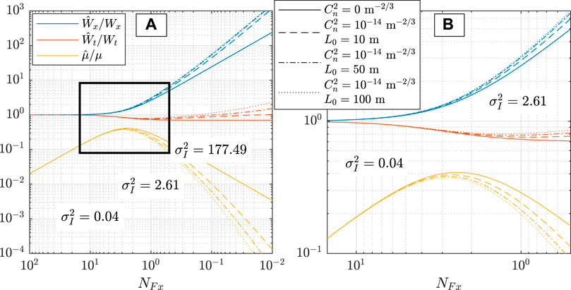
FIGURE 1. (A)
Starting with the free-space (solid) curves in Figure 1, we see that for NFx > 10, the twisted space-time beam is effectively in the source plane, with
Examining the turbulence (dashed, dashed-dotted, and dotted) curves, we generally observe the same behavior; however, the beam’s evolution described above is effectively pushed to the left, i.e., toward higher Fresnel numbers. Where the separation between free-space (diffractive) and turbulence-induced behavior occurs (in other words, at what NFx), of course, depends on
1. The beam’s size
2. After initially contracting, the pulse width
In atmospheric turbulence, the term containing the twist parameter μ tends to zero like z−2 (in free space, the term asymptotes to a constant value). For large z, the result is therefore
3. The x-t plane rotation
3 Validation
In this section, we validate Eq. 19 by generating, in simulation, twisted space-time beam field realizations and propagating those realizations through atmospheric turbulence phase screens. Before presenting and analyzing the results, we discuss the simulation setup.
3.1 Simulation setup
3.1.1 Numbers of grid points, spacings, trials, etc.
In these wave-optics simulations, we generated and propagated twisted space-time beam field realizations through independent instances of atmospheric turbulence. The Fresnel numbers for these simulations were NFx = 10, 5, 2.5, and 1. For each NFx, we computed the ensemble-averaged irradiance
3.1.2 Generating twisted space-time fields
We generated twisted space-time beam field realizations using the approach described in Ref. [31]. The technique utilizes Gori and Santarsiero’s integral criterion for genuine CSD functions and MCFs, colloquially known as the superposition rule [75, 76]. Specialized for our purposes, a thermal (or pseudo-thermal) twisted space-time beam field realization can be generated by evaluating the following superposition integral:
where r is a zero-mean, unit-variance, delta-correlated, complex Gaussian random function [31], and p and H are
The α, β, σx, and σt relate to the physical twisted space-time beam parameters in Eq. 13 via the relations [19, 35].
In the simulations, we produced twisted space-time beams with the following parameter values λc = 1 μm, Wx = Wy = 2 cm, δx = 0.9Wx, Wt = 1 ps, δt = 0.9Wt, and
3.1.3 Atmospheric turbulence
The index of refraction structure constant and outer scale for the atmospheric turbulence was
Note that we did not simulate the other turbulence conditions reported in Figure 1 due to computational constraints. Accurately simulating turbulence with a given outer scale requires phase screens that have physical dimensions on the order of L0. Simulating the L0 = 50 m and 100 m atm would have required grids that were (approximately) 25 and 100 times larger (in numbers of points), respectively, than those used in the L0 = 10 m simulations (see Section 3.1.1).
3.1.4 Procedure
On each Monte Carlo trial,
1. We generated a twisted space-time beam realization and an instance of atmospheric turbulence as described above.
2. We then Fourier transformed the twisted space-time beam realization to the ω domain using a fast Fourier transform (FFT) computed along the third dimension of U.
3. We propagated U to each of the 4, 5, 9, or 20 (depending on NFx) planes using the convolution form of the Fresnel diffraction integral (also known as the angular spectrum propagation method [78, 80]), which we evaluated using FFTs computed along U’s spatial dimensions.
4. In each plane, we converted the atmospheric phase screen in meters of OPL to radians using the ω values along the third dimension of U. We then applied the phase screen to the field and propagated U to the next plane.
5. Upon reaching the observation plane, we Fourier transformed the field back to the t domain using an FFT computed along U’s third dimension.
6. Lastly, we computed the trial irradiance
We repeated this procedure 1,000 times.
3.2 Results
Figures 2–4 show the results of the twisted space-time beam simulations. Figures 2, 3—which report the ensemble-averaged irradiances
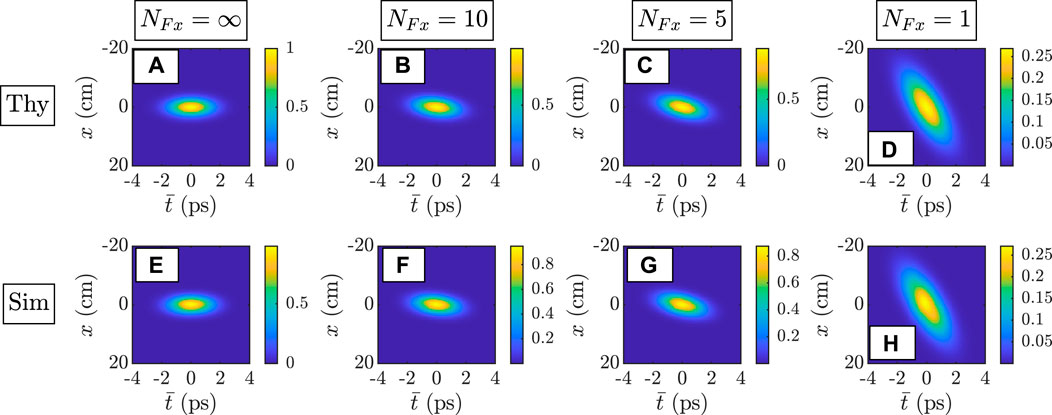
FIGURE 2. Ensemble-averaged irradiance

FIGURE 3. Ensemble-averaged irradiance
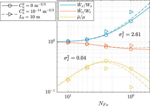
FIGURE 4. Theory [Eq. 19] and simulation
Inspection of Figure 3 reveals good agreement between simulation and theory in weak to moderately strong atmospheric turbulence [Figures 3B, C, F, and G]. In contrast, the agreement is rather poor in strong turbulence [Figures 3D, H]. This discrepancy is likely caused by the quadratic approximation we used to derive the MCF in Eq. 17 and subsequently
3.3 Experimental verification
Before concluding, we briefly discuss the process for experimentally verifying the theoretical and simulated results presented above. Twisted space-time beam field realizations can be physically synthesized using an apparatus known as a Fourier transform pulse shaper (FTPS) [1, 4, 9, 84–87]. An FTPS consists of two identical gratings separated by a 4f cylindrical lens (CL) system. At the center of the 4f system is a spatial light modulator (SLM). Assuming a pulsed laser beam is input into the FTPS, the first grating-CL-2f system spreads and maps the input beam’s spectrum into physical space at the SLM plane. The SLM modifies the field in the space-frequency (x-ω) domain, which is then transformed back to the space-time domain by the second grating-CL-2f system. Partial coherence manifests by incoherently summing many independent twisted space-time beam realizations.
Turbulence (besides outdoor experiments which are generally uncontrolled) can be controllably generated in the laboratory using several different methods [88]. Of these, phase plate/wheel [89–92] or hot-air [93, 94] techniques are the most germane, and systems employing those methods are easily capable of reproducing the turbulence conditions simulated above.
Lastly, to observe the beam’s behavior in x-t domain, we follow the procedure described in Refs. [1, 5]: The light at the output of the turbulence generator transits a grating-CL-2f system and then is measured by a detector. The detector measures the light’s spatially resolved spectrum averaged over many independent field and turbulence realizations, i.e.,
Note that this quantity is also referred to as the spectral density [58, 59, 71, 72]. Using Eq. 14, the spectral density relates to the MCF via
and consequently, the ensemble-averaged irradiance
4 Conclusion
In this paper, we focused on a recently introduced, partially coherent, space-time-coupled field known as a twisted space-time beam. Twisted space-time beams are similar to traditional twisted Gaussian Schell-model beams; however, instead of being spatially twisted (like the latter), the former possess a stochastic twist which couples their space and time dimensions. Like STOV beams, this spatiotemporal twist imbues twisted space-time beams with transverse (to the direction of propagation) angular momentum.
Generalizing the original research presented in Refs. [19, 20], here, we studied how twisted space-time beams behave as they propagate through atmospheric turbulence. Applying the extended Huygens–Fresnel principle, we derived the MCF for twisted space-time beams after propagating a distance z through atmospheric turbulence of arbitrary strength. From the MCF, we obtained the ensemble-averaged irradiance and quantified the effects of turbulence on beam size, pulse width, and space-time twist. We then simulated twisted space-time beam propagation through atmospheric turbulence to validate our theoretical analysis. The simulated results were found to be in good agreement with theory in weak-to-moderate turbulence. On the other hand, we observed rather poor agreement in strong turbulence, where our theoretical expression for the ensemble-averaged irradiance underestimated the effects of turbulence on the beam size, pulse width, and space-time twist. It did, however, accurately predict the trends of those parameters versus Fresnel number and turbulence strength.
Light with engineered space-time or spatiotemporal coupling is a new and exciting aspect of beam control research, with potential revolutionary uses in optical communications, optical tweezing, and quantum optics. While the free-space propagation characteristics of space-time-coupled beams are generally understood, much less is known about how these beams behave in random media. The results in this paper are a first step toward this goal.
Data availability statement
The original contributions presented in the study are included in the article/Supplementary Material, further inquiries can be directed to the corresponding author.
Author contributions
MH performed the tasks of conceptualization, formal analysis, investigation, methodology, validation, visualization, and writing.
Acknowledgments
The views expressed in this paper are those of the authors and do not reflect the official policy or position of the US Air Force, the Department of Defense, or the US government. MH would like to thank the Air Force Office of Scientific Research (AFOSR) Physical and Biological Sciences Branch (RTB) for supporting this work.
Conflict of interest
The author declares that the research was conducted in the absence of any commercial or financial relationships that could be construed as a potential conflict of interest.
Publisher’s note
All claims expressed in this article are solely those of the authors and do not necessarily represent those of their affiliated organizations, or those of the publisher, the editors and the reviewers. Any product that may be evaluated in this article, or claim that may be made by its manufacturer, is not guaranteed or endorsed by the publisher.
References
1. Kondakci HE, Abouraddy AF. Diffraction-free space-time light sheets. Nat Photon (2017) 11:733–40. doi:10.1038/s41566-017-0028-9
2. Yessenov M, Bhaduri B, Kondakci HE, Abouraddy AF. Weaving the rainbow: Space-time optical wave packets. Opt. Photonics News (2019) 30(5):34–41. doi:10.1364/OPN.30.5.000034
3. Bhaduri B, Yessenov M, Abouraddy AF. Anomalous refraction of optical spacetime wave packets. Nat Photon (2020) 14:416–21. doi:10.1038/s41566-020-0645-6
4. Yessenov M, Hall LA, Schepler KL, Abouraddy AF. Space-time wave packets. Adv Opt Photon (2022) 14:455–570. doi:10.1364/AOP.450016
5. Dallaire M, McCarthy N, Piché M. Spatiotemporal bessel beams: Theory and experiments. Opt Express (2009) 17:18148–64. doi:10.1364/OE.17.018148
6. Bliokh KY, Nori F. Spatiotemporal vortex beams and angular momentum. Phys Rev A (Coll Park) (2012) 86:033824. doi:10.1103/PhysRevA.86.033824
7. Jhajj N, Larkin I, Rosenthal EW, Zahedpour S, Wahlstrand JK, Milchberg HM. Spatiotemporal optical vortices. Phys Rev X (2016) 6:031037. doi:10.1103/PhysRevX.6.031037
8. Hancock SW, Zahedpour S, Goffin A, Milchberg HM. Free-space propagation of spatiotemporal optical vortices. Optica (2019) 6:1547–53. doi:10.1364/OPTICA.6.001547
9. Chong A, Wan C, Chen J, Zhan Q. Generation of spatiotemporal optical vortices with controllable transverse orbital angular momentum. Nat Photon (2020) 14:350–4. doi:10.1038/s41566-020-0587-z
10. Meng X, Hu Y, Wan C, Zhan Q. Optical vortex fields with an arbitrary orbital angular momentum orientation. Opt Lett (2022) 47:4568–71. doi:10.1364/OL.468360
11. Wan C, Chen J, Chong A, Zhan Q. Photonic orbital angular momentum with controllable orientation. Natl Sci Rev (2021) 9:nwab149. doi:10.1093/nsr/nwab149
12. Yao AM, Padgett MJ. Orbital angular momentum: Origins, behavior and applications. Adv Opt Photon (2011) 3:161–204. doi:10.1364/AOP.3.000161
13. Gao D, Ding W, Nieto-Vesperinas M, Ding X, Rahman M, Zhang T, et al. Optical manipulation from the microscale to the nanoscale: Fundamentals, advances and prospects. Light Sci Appl (2017) 6:e17039. doi:10.1038/lsa.2017.39
14. Padgett MJ. Orbital angular momentum 25 years on [Invited]. Opt Express (2017) 25:11265–74. doi:10.1364/OE.25.011265
15. Shen Y, Wang X, Xie Z, Min C, Fu X, Liu Q, et al. Optical vortices 30 years on: OAM manipulation from topological charge to multiple singularities. Light Sci Appl (2019) 8:90. doi:10.1038/s41377-019-0194-2
16. Angelsky OV, Bekshaev AY, Hanson SG, Zenkova CY, Mokhun , Jun Z. Structured light: Ideas and concepts. Front Phys (2020) 8:114. doi:10.3389/fphy.2020.00114
17. Yessenov M, Bhaduri B, Kondakci HE, Meem M, Menon R, Abouraddy AF. Non-diffracting broadband incoherent space-time fields. Optica (2019) 6:598–607. doi:10.1364/OPTICA.6.000598
18. Mirando A, Zang Y, Zhan Q, Chong A. Generation of spatiotemporal optical vortices with partial temporal coherence. Opt Express (2021) 29:30426–35. doi:10.1364/OE.431882
19. Hyde MW. Twisted space-frequency and space-time partially coherent beams. Sci Rep (2020) 10:12443. doi:10.1038/s41598-020-68705-9
20. Hyde IVMW. Twisted spatiotemporal optical vortex random fields. IEEE Photon J (2021) 13:1–16. doi:10.1109/JPHOT.2021.3066898
21. Ding C, Horoshko D, Korotkova O, Jing C, Qi X, Pan L. Source coherence-induced control of spatiotemporal coherency vortices. Opt Express (2022) 30:19871. doi:10.1364/OE.458666
22. Simon R, Mukunda N. Twisted Gaussian schell-model beams. J Opt Soc Am A (1993) 10:95–109. doi:10.1364/JOSAA.10.000095
23. Simon R, Sundar K, Mukunda N. Twisted Gaussian Schell-model beams. I. Symmetry structure and normal-mode spectrum. J Opt Soc Am A (1993) 10:2008. doi:10.1364/JOSAA.10.002008
24. Sundar K, Simon R, Mukunda N. Twisted Gaussian Schell-model beams. II. Spectrum analysis and propagation characteristics. J Opt Soc Am A (1993) 10:2017–23. doi:10.1364/JOSAA.10.002017
25. Simon R, Mukunda N. Twist phase in Gaussian-beam optics. J Opt Soc Am A (1998) 15:2373–82. doi:10.1364/JOSAA.15.002373
26. Ambrosini D, Bagini V, Gori F, Santarsiero M. Twisted Gaussian schell-model beams: A superposition model. J Mod Opt (1994) 41:1391–9. doi:10.1080/09500349414551331
27. Gori F, Santarsiero M, Borghi R, Vicalvi S. Partially coherent sources with helicoidal modes. J Mod Opt (1998) 45:539–54. doi:10.1080/09500349808231913
28. Friberg AT, Tervonen E, Turunen J. Interpretation and experimental demonstration of twisted Gaussian Schell-model beams. J Opt Soc Am A (1994) 11:1818–26. doi:10.1364/JOSAA.11.001818
29. Wang H, Peng X, Liu L, Wang F, Cai Y, Ponomarenko SA. Generating bona fide twisted Gaussian Schell-model beams. Opt Lett (2019) 44:3709–12. doi:10.1364/OL.44.003709
30. Tian C, Zhu S, Huang H, Cai Y, Li Z. Customizing twisted Schell-model beams. Opt Lett (2020) 45:5880–3. doi:10.1364/OL.405149
31. Hyde MW. Stochastic complex transmittance screens for synthesizing general partially coherent sources. J Opt Soc Am A (2020) 37:257–64. doi:10.1364/JOSAA.381772
32. Wang H, Peng X, Zhang H, Liu L, Chen Y, Wang F, et al. Experimental synthesis of partially coherent beam with controllable twist phase and measuring its orbital angular momentum. Nanophotonics (2021) 11:689–96. doi:10.1515/nanoph-2021-0432
33. Zhang Y, Zhang X, Wang H, Ye Y, Liu L, Chen Y, et al. Generating a twisted Gaussian Schell-model beam with a coherent-mode superposition. Opt Express (2021) 29:41964–74. doi:10.1364/OE.446160
34. Gori F, Santarsiero M. Twisted Gaussian Schell-model beams as series of partially coherent modified Bessel-Gauss beams. Opt Lett (2015) 40:1587–90. doi:10.1364/OL.40.001587
35. Mei Z, Korotkova O. Random sources for rotating spectral densities. Opt Lett (2017) 42:255–8. doi:10.1364/OL.42.000255
36. Borghi R. Twisting partially coherent light. Opt Lett (2018) 43:1627–30. doi:10.1364/OL.43.001627
37. Gori F, Santarsiero M. Devising genuine twisted cross-spectral densities. Opt Lett (2018) 43:595–8. doi:10.1364/OL.43.000595
38. Serna J, Movilla JM. Orbital angular momentum of partially coherent beams. Opt Lett (2001) 26:405–7. doi:10.1364/OL.26.000405
39. Kim SM, Gbur G. Angular momentum conservation in partially coherent wave fields. Phys Rev A (Coll Park) (2012) 86:043814. doi:10.1103/PhysRevA.86.043814
41. Stahl CSD, Gbur G. Twisted vortex Gaussian Schell-model beams. J Opt Soc Am A (2018) 35:1899–906. doi:10.1364/JOSAA.35.001899
42. Lin Q, Cai Y. Tensor ABCD law for partially coherent twisted anisotropic Gaussian-Schell model beams. Opt Lett (2002) 27:216–8. doi:10.1364/OL.27.000216
43. Cai Y, He S. Propagation of a partially coherent twisted anisotropic Gaussian Schell-model beam in a turbulent atmosphere. Appl Phys Lett (2006) 89:041117. doi:10.1063/1.2236463
44. Wang F, Cai Y. Second-order statistics of a twisted Gaussian Schell-model beam in turbulent atmosphere. Opt Express (2010) 18:24661–72. doi:10.1364/OE.18.024661
45. Wang F, Cai Y, Eyyuboğlu HT, Baykal Y. Twist phase-induced reduction in scintillation of a partially coherent beam in turbulent atmosphere. Opt Lett (2012) 37:184–6. doi:10.1364/OL.37.000184
46. Cai Y, Zhu S. Orbital angular moment of a partially coherent beam propagating through an astigmatic ABCD optical system with loss or gain. Opt Lett (2014) 39:1968. doi:10.1364/ol.39.001968
47. Charnotskii M. Transverse linear and orbital angular momenta of beam waves and propagation in random media. J Opt (2018) 20:025602. doi:10.1088/2040-8986/aa9f50
48. Wang J, Wang H, Zhu S, Li Z. Second-order moments of a twisted Gaussian Schell-model beam in anisotropic turbulence. J Opt Soc Am A (2018) 35:1173–9. doi:10.1364/JOSAA.35.001173
49. Zhou M, Fan W, Wu G. Evolution properties of the orbital angular momentum spectrum of twisted Gaussian Schell-model beams in turbulent atmosphere. J Opt Soc Am A (2020) 37:142–8. doi:10.1364/JOSAA.37.000142
50. Liu Z, Wan L, Zhou Y, Zhang Y, Zhao D. Progress on studies of beams carrying twist. Photonics (2021) 8:92. doi:10.3390/photonics8040092
51. Ponomarenko SA. Classical entanglement of twisted random light propagating through atmospheric turbulence [Invited]. J Opt Soc Am A (2022) 39:C1. C1–C5. doi:10.1364/JOSAA.465410
52. Bliokh KY. Spatiotemporal vortex pulses: Angular momenta and spin-orbit interaction. Phys Rev Lett (2021) 126:243601. doi:10.1103/PhysRevLett.126.243601
53. Hancock SW, Zahedpour S, Milchberg HM. Mode structure and orbital angular momentum of spatiotemporal optical vortex pulses. Phys Rev Lett (2021) 127:193901. doi:10.1103/PhysRevLett.127.193901
54. Lutomirski RF, Yura HT. Propagation of a finite optical beam in an inhomogeneous medium. Appl Opt (1971) 10:1652–8. doi:10.1364/AO.10.001652
55. Fante RL, Wolf E. VI wave propagation in random media: A system approach. Opt (Elsevier), Prog Opt (1985) 22:341–98. chap. 6. doi:10.1016/S0079-6638(08)70152-5
56. Ishimaru A. Wave propagation and scattering in random media. Piscataway, NJ: IEEE Press (1999). p. 600.
57. Andrews LC, Phillips RL. Laser beam propagation through random media. 2nd ed. Bellingham, WA: SPIE Press (2005).
58. Mandel L, Wolf E. Optical coherence and quantum optics. New York, NY: Cambridge University (1995).
59. Lajunen H, Vahimaa P, Tervo J. Theory of spatially and spectrally partially coherent pulses. J Opt Soc Am A (2005) 22:1536–45. doi:10.1364/josaa.22.001536
60. Fante R. Electromagnetic beam propagation in turbulent media. Proc IEEE (1975) 63:1669–92. doi:10.1109/PROC.1975.10035
61. Fante R. Electromagnetic beam propagation in turbulent media: An update. Proc IEEE (1980) 68:1424–43. doi:10.1109/PROC.1980.11882
62. Fante RL. Two-position, two-frequency mutual-coherence function in turbulence. J Opt Soc Am (1981) 71:1446–51. doi:10.1364/JOSA.71.001446
63. Charnotskii M. Extended huygens-fresnel principle and optical waves propagation in turbulence: Discussion. J Opt Soc Am A (2015) 32:1357–65. doi:10.1364/JOSAA.32.001357
64.M Abramowitz, and IA Stegun, editors. Handbook of mathematical functions with formulas, graphs, and mathematical tables. Washington, DC: National Bureau of Standards (1964).
65. Gradshteyn IS, Ryzhik IM. Table of integrals, series, and products. 7th ed. Burlington, MA: Academic Press (2007).
66. Belafhal A, Chib S, Khannous F, Usman T. Evaluation of integral transforms using special functions with applications to biological tissues. Comp Appl Math (2021) 40:156. doi:10.1007/s40314-021-01542-2
67. Young CY, Andrews LC, Ishimaru A. Time-of-arrival fluctuations of a space–time Gaussian pulse in weak optical turbulence: An analytic solution. Appl Opt (1998) 37:7655–60. doi:10.1364/AO.37.007655
68. Young CY. Broadening of ultrashort optical pulses in moderate to strong turbulence. In: JC Ricklin, and DG Voelz, editors. Free-space laser communication and laser imaging II, 4821. Seattle, Washington, USA: International Society for Optics and Photonics SPIE (2002). p. 74–81. doi:10.1117/12.452061
69. Gbur G, Wolf E. Spreading of partially coherent beams in random media. J Opt Soc Am A (2002) 19:1592–8. doi:10.1364/JOSAA.19.001592
70. Gbur G. Partially coherent beam propagation in atmospheric turbulence [Invited]. J Opt Soc Am A (2014) 31:2038–45. doi:10.1364/JOSAA.31.002038
73. Wang F, Liu X, Cai Y. Propagation of partially coherent beam in turbulent atmosphere: A review (invited review). Prog Electromagn Res (2015) 150:123–43. doi:10.2528/PIER15010802
74. Wan L, Zhao D. Controllable rotating Gaussian Schell-model beams. Opt Lett (2019) 44:735–8. doi:10.1364/OL.44.000735
75. Gori F, Santarsiero M. Devising genuine spatial correlation functions. Opt Lett (2007) 32:3531–3. doi:10.1364/OL.32.003531
76. Martínez-Herrero R, Mejías PM, Gori F. Genuine cross-spectral densities and pseudo-modal expansions. Opt Lett (2009) 34:1399–401. doi:10.1364/OL.34.001399
77. Martin JM, Flatté SM. Intensity images and statistics from numerical simulation of wave propagation in 3-D random media. Appl Opt (1988) 27:2111–26. doi:10.1364/AO.27.002111
78. Schmidt JD. Numerical simulation of optical wave propagation with examples in MATLAB. Bellingham, WA: SPIE Press (2010).
79. Jarem JM, Banerjee PP. Computational methods for electromagnetic and optical systems. 2nd ed. Boca Raton, FL: CRC Press (2011).
81. Lane RG, Glindemann A, Dainty JC. Simulation of a Kolmogorov phase screen. Waves in Random Media (1992) 2:209–24. doi:10.1088/0959-7174/2/3/003
82. Frehlich R. Simulation of laser propagation in a turbulent atmosphere. Appl Opt (2000) 39:393–7. doi:10.1364/AO.39.000393
83. Fante RL. Some physical insights into beam propagation in strong turbulence. Radio Sci (1980) 15:757–62. doi:10.1029/RS015i004p00757
84. Weiner AM. Femtosecond pulse shaping using spatial light modulators. Rev Sci Instrum (2000) 71:1929–60. doi:10.1063/1.1150614
85. Ding C, Koivurova M, Turunen J, Setälä T, Friberg AT. Coherence control of pulse trains by spectral phase modulation. J Opt (2017) 19:095501. doi:10.1088/2040-8986/aa7b5e
87. Torres-Company V, Lancis J, Andrés P. Space-time analogies in optics. In: E Wolf, editor. Prog. Opt., 56. Elsevier (2011). p. 1–80. chap. 1. doi:10.1016/B978-0-444-53886-4.00001-0
88. Jolissaint L. Optical turbulence generators for testing astronomical adaptive optics systems: A review and designer guide. Publ Astron Soc Pac (2006) 118:1205–24. doi:10.1086/507849
89. Rodenburg B, Mirhosseini M, Malik M, Magaña-Loaiza OS, Yanakas M, Maher L, et al. Simulating thick atmospheric turbulence in the lab with application to orbital angular momentum communication. New J Phys (2014) 16:033020. doi:10.1088/1367-2630/16/3/033020
90. Rickenstorff C, Rodrigo JA, Alieva T. Programmable simulator for beam propagation in turbulent atmosphere. Opt Express (2016) 24:10000–12. doi:10.1364/OE.24.010000
91. Dayton D, Spencer M, Hassall A, Rhoadarmer T. Distributed-volume optical disturbance generation in a scaled-laboratory environment using nematic liquid-crystal phase modulators. In: JJ Dolne, and PJ Bones, editors. Unconventional and indirect imaging, image reconstruction, and wavefront sensing 2018, 10772. San Diego, California, USA: International Society for Optics and Photonics SPIE (2018). p. 107720H. doi:10.1117/12.2319968
92. Joo JY, Han SG, Lee JH, Rhee HG, Huh J, Lee K, et al. Development and characterization of an atmospheric turbulence simulator using two rotating phase plates. Curr Opt Photon (2022) 6:445–52.
93. Keskin O, Jolissaint L, Bradley C. Hot-air optical turbulence generator for the testing of adaptive optics systems: Principles and characterization. Appl Opt (2006) 45:4888–97. doi:10.1364/AO.45.004888
Keywords: atmospheric turbulence, coherence, random media, random fields, space-time coupling, spatiotemporal coupling, statistical optics
Citation: Hyde IV MW (2023) The behavior of partially coherent twisted space-time beams in atmospheric turbulence. Front. Phys. 10:1055401. doi: 10.3389/fphy.2022.1055401
Received: 27 September 2022; Accepted: 02 December 2022;
Published: 09 January 2023.
Edited by:
Muhsin Caner Gokce, TED University, TurkeyReviewed by:
Serkan Sahin, TED University, TurkeyGuoquan Zhou, Zhejiang Agriculture and Forestry University, China
Copyright © 2023 Hyde IV. This is an open-access article distributed under the terms of the Creative Commons Attribution License (CC BY). The use, distribution or reproduction in other forums is permitted, provided the original author(s) and the copyright owner(s) are credited and that the original publication in this journal is cited, in accordance with accepted academic practice. No use, distribution or reproduction is permitted which does not comply with these terms.
*Correspondence: Milo W. Hyde IV, milo.hyde@afit.edu