Evaluation of the Heterogeneous Spatial Distribution of Population and Stores/Facilities by Multifractal Analysis

1. Introduction

Fractality has been observed in various spatial distributions relating to the morphology of cities, e.g., population, buildings, land price, and street networks [1–10]. Fractality is represented by the nature where the mass (e.g., the population) in a region exhibits power law dependence on the size of the region. The power-law exponent is called the fractal dimension [11]. The abovementioned spatial distributions also exhibit heterogeneity in fractality in the sense that the locally measured fractal dimension around each spot diverges in the structure, known as multifractality [4, 12, 13].

The location of stores/facilities should depend on and, in turn, affect the spatial distribution of the population. People may choose the location of their settlement based on the availability and variety of stores/facilities. On the other hand, companies may invest in the construction of stores/facilities to secure employers and customers [14]. It is known that the nature of agglomeration of stores/facilities depends on their type. For example, previous studies showed that facilities relating to businesses offering professional services tend to concentrate in areas with a large population [14–16]. One of these studies evaluated the concentration by investigating the scaling law between the population and densities of facilities, showing that the number of facilities in a city increases with a power of the population in the city [16]. The scaling law is a universal pattern observed in urban morphology, e.g., accessibility, road surface, and crime [16–21]. It should be interesting to see whether the agglomeration of stores/facilities exhibits multifractality, another urban-related feature.

If the spatial distribution of stores/facilities exhibits multifractality, multifractal analysis can be performed on the structure and is a strong tool to quantify the feature of it. In multifractal analysis, the resulted curve exhibits the correspondence between the locally measured fractal dimension, called singularity strength α, and the fractal dimension of the arrangement of spots that exhibit the singularity strength α, called spectrum f(α) [4, 13].

Besides multifractal analysis, various methods have been applied to evaluate spatial distributions including that of the population and stores/facilities. Average nearest neighbor (ANN), which is the averaged distance to the nearest point, is an indicator of the spatial clustering [22–24]. The distribution of nearest neighbor distance is also used to evaluate the qualitative feature of spatial structure [24, 25]. On the other hand, when grid lines are drawn on the space, probability of finding neighboring cells both of which are occupied is often calculated to assess the degree of clustering [26, 27]. Regarding the industrial coagglomeration between two industries, the extent to which the facilities of these industries are in the same region is evaluated [14, 28]. Compared to these methods, an advantage of multifractal analysis should be that it can demonstrate both local and global features of the spatial distribution [9]. By multifractal analysis, the strength of local concentration can be captured by the singularity strength. The global view of the arrangement of spots with each level of concentration, on the other hand, is incorporated into the spectrum.

In this study, we aim to (1) determine if the spatial distributions of stores/facilities in various categories exhibit multifractality, and if so, (2) determine the characteristics captured by the multifractal properties of each spatial distribution.

We chose the largest metropolitan area in Japan, the Kantō area, as the object of our analysis. We investigated the multifractal properties of the spatial distributions of the population and stores/facilities in Kantō. Our analysis showed that the spatial distribution of stores/facilities in some categories exhibit multifractality, as does that of the population. Though these spatial distributions are on the same geographical substrate, their multifractal properties are significantly different from each other.

This paper is organized as follows. The principles of fractal geometry, multifractality, and the generalized dimension, as well as the methods of our analysis are presented in section 2. We show the results of multifractal analysis of the spatial distributions in section 3. We also compare the multifractal properties of these spatial distributions and highlight the information extractable from the multifractal measures of the spatial distributions. We discuss the results in section 4.

2. Materials and Methods

2.1. Data

Data for the spatial distributions of the population and stores/facilities were extracted from the Japanese 100-Meter Estimated Mesh Data of the 2015 National Censuses (Zenrin Marketing Solutions Co., Ltd.) and the Corporate Telephone Directory Database Telepoint with Coordinates (Telepoint Pack! provided by ZENRIN Co., Ltd.) of 2017, respectively. The former dataset contains data on the estimated population in each mesh. The length of each side of a mesh is ~100 m, while the exact size is 3 s in the latitude direction and 4.5 s in the longitude direction. The latter dataset contains the geospatial information of each store/facility. Stores/facilities are categorized hierarchically. In the largest classification, which we adopted, there are 39 categories as shown in Table 1.

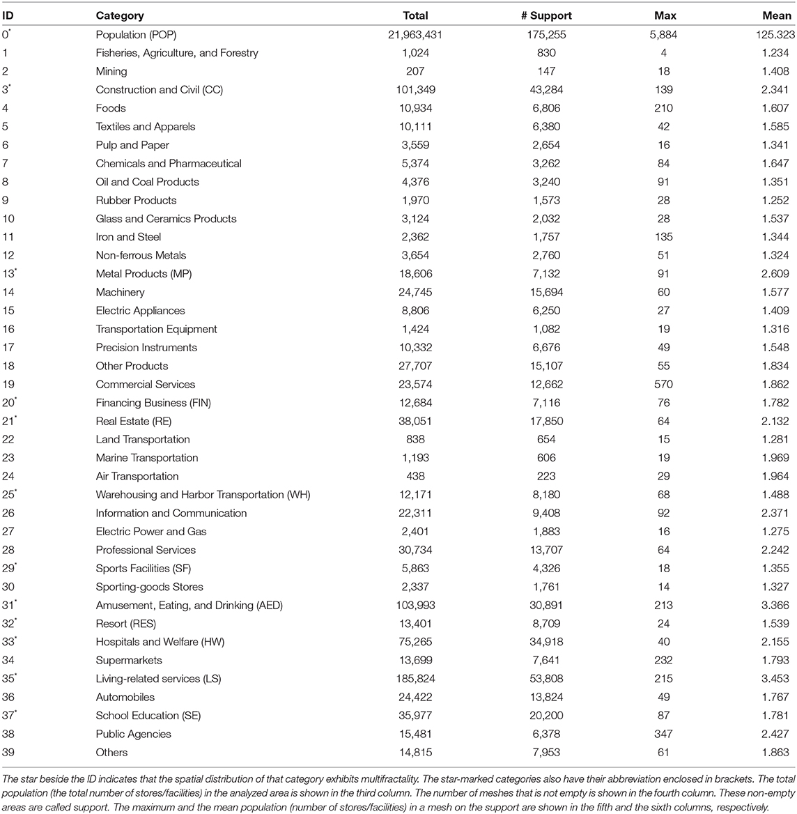
Table 1. Data summary. For each category, the ID and the name of the category are shown in the first and second columns, respectively.

The analyzed area is a part of Kantō in Japan, that includes the capital, Tokyo, and a major industrial area, the Keihin industrial area. The range of the latitude is from 35°29′54″ to 35°55′30″ and that of the longitude is from 139°16′52.5″ to 139°55′16.5″ (Figure 1). There are 2⁹ × 2⁹ (= 262,144) meshes inside this region.

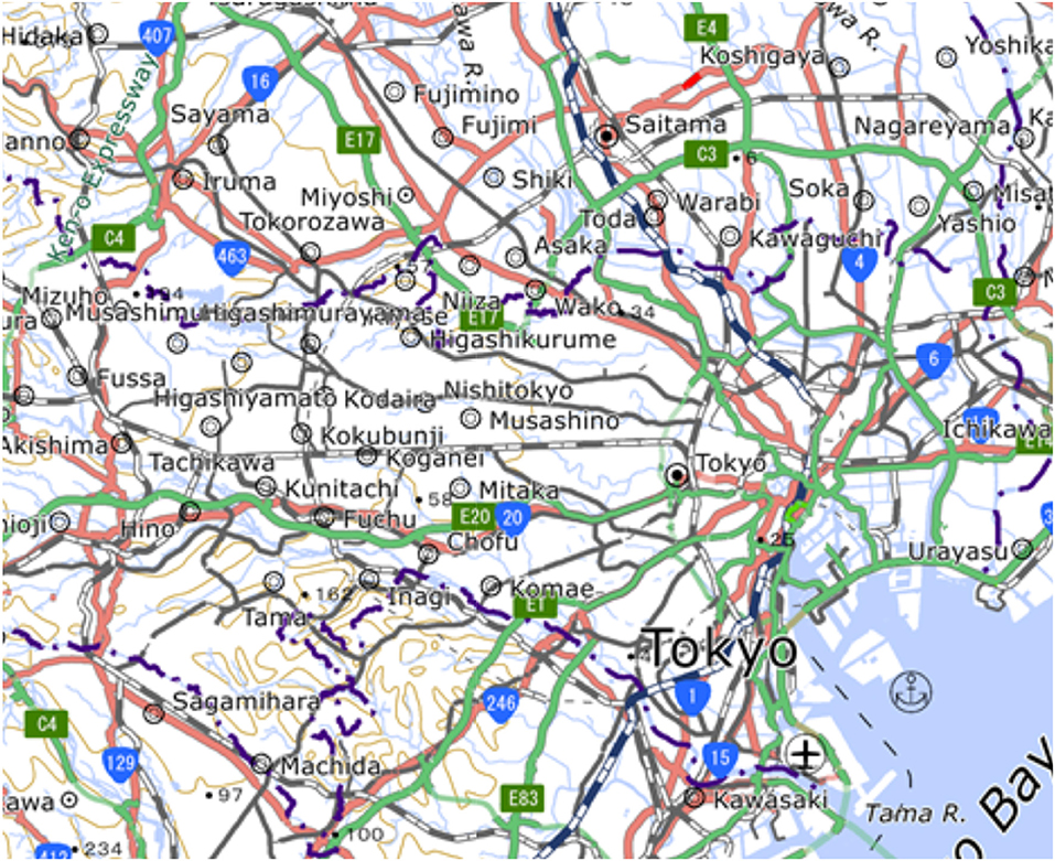
Figure 1. Map of the analyzed area (1:1,000,000 INTERNATIONAL MAP, Geospatial Information Authority of Japan).

Table 1 shows a summary of the data analyzed in this study. The total population (the total number of stores/facilities) in the analyzed area and the number of non-empty meshes are shown in the third and fourth columns, respectively. Here, the meshes/boxes with non-zero populations (stores/facilities) are called support. The maximum and the mean population (number of stores/facilities) in a mesh on the support are shown from the fifth to the sixth columns.

Figure 2A shows the spatial distribution of the population in the analyzed area. The logarithm of the proportion of the population in each mesh to the total population is represented by the heatmap. The other panels (B–L) show the spatial distributions of stores/facilities in 11 categories.

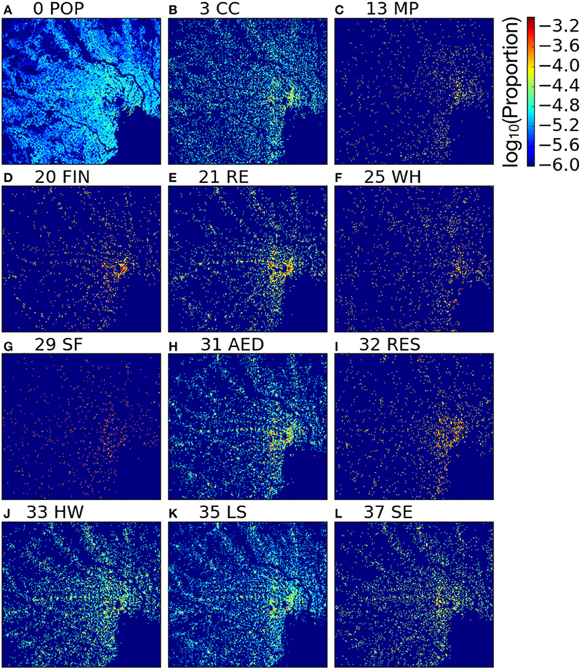
Figure 2. Spatial distributions of the population and stores/facilities in the analyzed area. (A) The spatial distribution of the population. (B–L) The spatial distributions of stores/facilities in 11 categories: (B) 3CC (Construction and Civil); (C) 13MP (Metal Products); (D) 20FIN (Financing Business); (E) 21RE (Real Estate); (F) 25WH (Warehousing and Harbor Transportation); (G) 29SF (Sports Facilities); (H) 31AED (Amusement, Eating, and Drinking); (I) 32RES (Resort); (J) 33HW (Hospitals and Welfare); (K) 35LS (Living-related Services); (L) 37SE (School Education). For the other categories, the spatial distributions are shown in Figures S1, S2. The color stands for the value of log₁₀[(the population in the mesh)/(the total population)] for each mesh in (A). The number of stores/facilities is used instead of the population in (B–L). Each mesh is a 100-m mesh as described in section 2.

2.2. Multifractality

We briefly introduce the concepts of fractal geometry and multifractality. There are several ways of defining fractals and multifractals; we present one of them here [9, 11–13, 29]. Additionally, we limit our explanation to structures embedded in ℝ², while higher dimensions of fractal and multifractal structures can be generally defined.

When a mass (m(ε)) composing a structure within a region of size ε increases with ε according to m(ε) ~ ε^D, the structure is regarded as having fractal characteristics. Here, the “size” is, for example, the length of a side if the region is a square. The exponent D is the fractal dimension of the structure. A more precise definition of the fractal dimension of a structure X is the one by the following box-counting method [11]. Let us assume that a structure X is covered with boxes of size ε. Let N(ε) be the minimum number of such boxes required to cover the structure. Then the box-counting dimension D is defined as:

We introduce multifractality. We again consider a set X and a function μ on X that gives a quantity, such as the density, at each point x ∈ X. Let us assume that X is divided by square boxes that have the same size ε. For the i-th box of size ε, C_{i, ε}, the value P_{i, ε} is called the probability measure on the box:

If P_{i, ε} and ε have the following power-law relationship for any i:

then fractality can be seen around each point of X. Here we assume that the exponent α diverges in X and let N(ε, α) be the number of boxes that satisfy $P_{i,\epsilon }~{\epsilon }^{\tilde{\alpha }}$ where $\tilde{\alpha }\in \left[\alpha ,\alpha +\Delta \alpha \right]$. If N(ε, α) decreases with ε as

the set X can be regarded as having a multifractal structure. Exponent α, which can be regarded as the local fractal dimension, is called the singularity strength. On the other hand, exponent f(α) stands for the box-counting dimension of the set of points with the singularity strength α. This dimension f(α) is called the spectrum. In this paper, the curve of (α, f(α)) is called the multifractal curve. Figure 3 is an example of the relationship between α and f(α) in the spatial distribution of the population (Figure 2A). Each panel in Figure 3 shows the units that exhibit the singularity strength α within the range shown on each panel. We derived the singularity strength of each unit by estimating the exponent in the following relationship $P_{i,\epsilon }~{\epsilon }^{\alpha }$ (see Equation 3). The box-counting dimension of the arrangement of units with the singularity strength α, f(α), was also derived based on Equation (4) when the power-law relationship in the equation holds. For example, units with the singularity strength α within [1.85, 1.90) are rare. Also, the arrangement of such units is curve-like (i.e., a one-dimensional shape) and exhibits a low box-counting dimension f(α) ~ 1.60. On the other hand, the arrangement of units with the singularity strength α within [2.05, 2.10) spans a two dimensional region and exhibits a high box-counting dimension that is about 2.

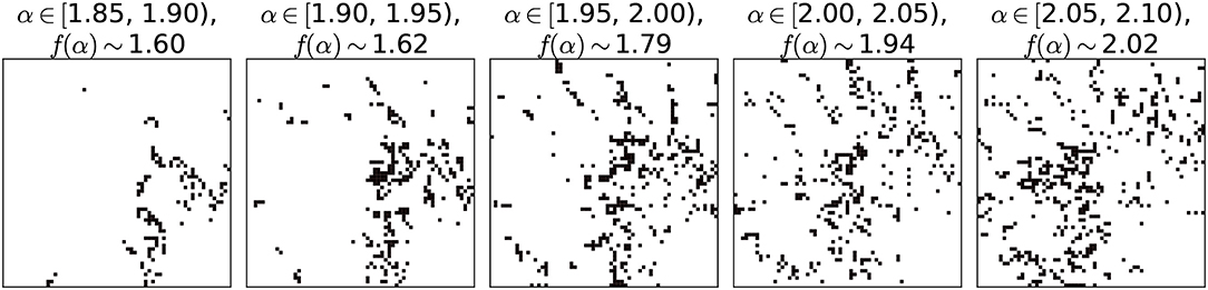
Figure 3. Example of the singularity strength α and the spectrum f(α). In each panel, units that have the singularity strength α within the range mentioned at the top of the panel are shown. Here the size of each unit is 2³/2⁹ on one side, and α is derived based on Equation (3). Also, the spectrum f(α) is derived based on Equation (4), only when the power-law relationship in Equation (4) holds.

2.3. Generalized Dimension

We introduce the generalized dimension and explain the relationship between the singularity strength, the spectrum, and the generalized dimension [29, 30]. The q-th generalized dimension D_q is defined as follows. First, we define τ_q as

Then the generalized dimension D_q for q ≠ 1 is defined as

In the case of q = 1,

In the summation on the right-hand side of each of Equations (5), (7), let the i-th term be summed when the i-th box is not empty, i.e., P_{i, ε} ≠ 0. Here, the generalized dimension is equal to the box-counting dimension of the support D when q is zero.

It is known that the following values of α_q and f(α_q) give the approximation of the pair of α and f(α) for each q:

2.4. Method of Analysis

In this study, we are concerned with finite morphologies that do not contain infinitesimal structures as the smallest unit of our data is a 100-m mesh. Therefore, we cannot rigorously calculate the generalized dimension, singularity strength, and spectrum. Instead, we consider the range of q and ε in which the structure can be regarded as exhibiting (multi)fractality, by evaluating the range of q and ε in which the following relationship holds:

Thus, we examine the linearity of the relationship between $log\sum _i{P}_{i,\epsilon }^q$ and logε by the frequently used method [3, 4, 7, 8, 31–34]. Then we regard d as τ_q by Equation (5) when $log\sum _i{P}_{i,\epsilon }^q~dlog\epsilon +(\mathrm{\text{const.}})$.

In our analysis, we assign the size of one side of a 100-m mesh to ε = 1/2⁹. Grid lines are drawn on the analyzed area so that it is covered by non-overlapping boxes with the same size [3, 7]. As the size of boxes, we consider ε = 1/2⁹, 2/2⁹, 2²/2⁹, ..., 1. We define the probability measure P_{i, ε} on the i-th box with the size ε as the proportion of the population (the number of stores/facilities) in the i-th box to the total population (the total number of stores/facilities).

Subsequently, for the population, we evaluate the linearity of the relationship between $log\sum _i{P}_{i,\epsilon }^q$ and logε for various ranges of ε and q as shown in Figure 4. Regarding the criterion for this linearity, we examined whether or not the coefficient of determination of the linear regression, R², exceeds 0.99. A linear relationship was not observed when q takes a negative value and when the range of ε includes values <2³/2⁹. Consequently, we considered the range of ε from 2³/2⁹ to 2⁹/2⁹, and the range of q from 0 to 20. We performed a multifractal analysis on these ranges of ε and q for the spatial distribution of the population. Furthermore, for the spatial distribution of stores/facilities in each category, we examined multifractality on the same ranges of ε and q as that for the population. Plots of $log\sum _i{P}_{i,\epsilon }^q$ against logε for all categories of stores/facilities are shown in Figures S3, S4. The star marker was added beside the ID in the first column of Table 1 if the category showed multifractality in the spatial distribution. Also, the spatial distribution of such categories are shown in Figures 2B–L. In this figure and in the following discussion, abbreviations are used for these categories—the abbreviation of each category is enclosed by brackets after the name of the category in the second column of Table 1.

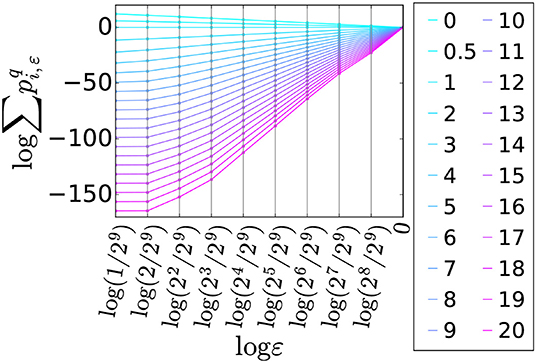
Figure 4. $log\sum _i{P}_{i,\epsilon }^q$ vs. logε for each q. The color of the plots correspond to the value of q in the legend.

We obtained τ_q as the slope of the linear regression of $log\sum _i{P}_{i,\epsilon }^q$ by logε, and derived D_q from Equations (6, 7). To derive the singularity strength α_q and the spectrum f(α_q), we used the following formulae:

where ${\mu }_{i,\epsilon ,q}=P_{i,\epsilon }^q/\sum _j{P}_{j,\epsilon }^q$. These formulae can be directly derived from Equation (5), (8), and (9) [12, 35, 36]. We obtained α_q by the linear regression between $\sum _i{\mu }_{i,\epsilon ,q}log{P}_{i,\epsilon }$ and logε, and obtained f(α_q) by the linear regression between $\sum _i{\mu }_{i,\epsilon ,q}log{\mu }_{i,\epsilon ,q}$ and logε.

3. Results

3.1. Density of Units and Multifractality

As we briefly mentioned in section 2.4, multifractality could not be observed for the spatial distribution of the population when the value of q is negative. Knowledge of the relationship between the densities in a unit, the value of q, and the multifractal measures is helpful for interpreting the results of the multifractal analysis. In Equation (5) for τ_q, a larger value of q corresponds to a greater contribution of the boxes with large probability measures P_{i, ε} to the sum. Therefore, the boxes with high densities are significantly incorporated into the calculation of the q-th generalized dimension D_q when the value of q is large, see Equation (6). Note that no differences in density is considered when q = 0. The pair of the singularity strength and the spectrum also has a relationship with q by Equations (8), (9). Therefore, the multifractal measures of D_q, α_q, and f(α_q) for a large q, significantly reflect those units with high densities. The fact that multifractality was only observed in the spatial distribution of the population with positive q values, indicates that multifractality cannot be observed in sparsely populated areas.

3.2. Generalized Dimension

Figure 5 shows the q-th generalized dimension vs. q for the population and stores/facilities in four categories: 20FIN, 25WH, 31AED, and 33HW. The generalized dimension for stores/facilities in the other categories is shown in Figure S5. As mentioned before, the generalized dimension for q = 0, D₀, is equal to the box-counting dimension of the support. For each category, the value of D₀ is close to 2, which is the dimension of ℝ² to which each spatial distribution is embedded. The rate of decline in the generalized dimension with q significantly varies between the categories. The generalized dimension for 20FIN drops dramatically with q, while that of the population decreases minimally with q. In the cases of 25WH and 33HW, the decline of the generalized dimension is milder than that of 20FIN and 31AED. Considering the relationship between the value of q and the densities in the boxes, |ΔD₂₀|: = |D₂₀ − D₀| can be one of the indicators for the strength of the heterogeneity in spatial density distribution, and 20FIN and 31AED can be regarded as having strong heterogeneity in spatial distributions.

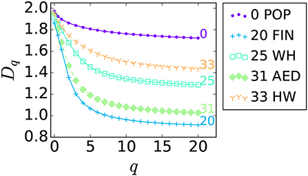
Figure 5. q-th generalized dimension vs. q for the population and stores/facilities in four categories: 20FIN, 25WH, 31AED, and 33HW. The generalized dimension for stores/facilities in the other categories are shown in Figure S5.

3.3. Multifractal Curve

The multifractal curves are shown in Figure 6A. Before we investigate each multifractal curve, let us revisit the relationship between the densities in a unit and the value of q, and the singularity strength α_q [9]. Recall that each point on the multifractal curve can be derived for each q (Equations 11, 12). Generally speaking, in each multifractal curve, the greater is the value of q, the lower is the value of α_q, i.e., the plot of a multifractal curve proceeds to the left as the value of q increases. Therefore, by the relationship between the value of q and the densities in the units, a unit with a high density tends to have a small singularity strength—we can observe this by comparing Figure 2A with Figure 3. An interpretation is that around a unit with a density significantly higher than the surroundings, the probability measure P_{i, ε} does not increase rapidly by expanding the area, and vice versa (see Equation 3). Figure 7 explains this interpretation. Let us assume that each of the gray units has a constant density. Only the i-th unit is filled in the case of panel (A), while all the units are filled in the case of panel (B). The singularity strength of the i-th unit in panel (A) is 0, since the probability measure of the square boxes emphasized by the thick line, that expands around the i-th unit, does not increase with the size ε of the box and remains at the same value. On the other hand, the probability measure on these boxes changes according to the square of ε, and the singularity strength of the i-th unit is 2, in panel (B). Though panels (A) and (B) are extreme examples, these diagrams suggest that a unit with a density significantly higher than the surrounding units can have a low singularity strength.

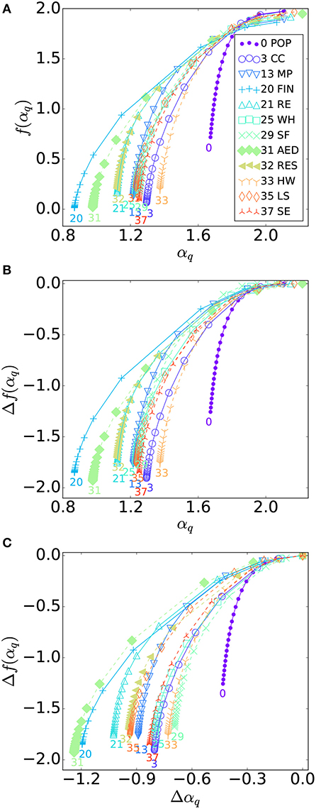
Figure 6. (A) Multifractal curve. The pair of the singularity strength (abscissa) and the spectrum (ordinate), (α_q, f(α_q)), for each q of the population and stores/facilities. Each multifractal curve is also separately shown in Figure S6. (B) Δf(α_q) vs. α_q, where Δf(α_q): = f(α_q) − f(α₀). (C) Δf(α_q) vs. Δα_q, where Δα_q: = α_q − α₀.

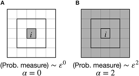
Figure 7. Schematic image of the singularity strength and the densities in a unit. Each of the gray-colored units has the same density, i.e., has the same probability measure ρ. (A) Only the i-th unit has non-zero density and the other units are empty. The probability measure of the box remains ρ, even when the size of the box ε increases as emphasized by the thick line. Therefore, the singularity strength of the i-th unit is 0. (B) All units are filled. The probability measure of the box is ρ, 9ρ, and 25ρ, for the smallest, the second smallest and the largest boxes (emphasized by the thick line), respectively. Thus, the singularity strength of the i-th unit is 2.

Therefore, in Figure 6A, multifractal curves with a significantly low singularity strength α_q, such as 20FIN and 31AED, indicate the existence of units with a density much higher than the surroundings. Also, the spectrum f(α_q) is quite low for small singularity strengths α_q in the cases of 20FIN and 31AED. Recall that the spectrum f(α_q) represents the box-counting dimension of the arrangement of units with the singularity strength α_q. The pair of small α_q and f(α_q), thus, is an indication that there are a few isolated units, each with an extremely high density.

Multifractal curves contain information not only at small singularity strengths but also across the entire range. The multifractal curve of 13MP has similar α_q and f(α_q) values with that of 25WH, 29SF, 35LS, and 37SE when α_q is quite small. However, in the mid-range of α_q, the value of f(α_q) for 13MP is significantly greater than that of the others. Therefore, in the case of 13MP, units with a mid-range density (compared to the surroundings) remain concentrated compared to the case of the other categories. This may correspond to the yellowish units gathered on the right of panel (C) in Figure 2. On the other hand, a feature of the multifractal curve of the population is that neither α_q nor f(α_q) declines rapidly with q. This corresponds to the following features of the spatial distribution of the population: The densities in the units does not widely diverge and the arrangement of the units with each density does not change dramatically with the density (Figure 2A).

Figure 6B shows the plots of Δf(α_q): = f(α_q) − f(α₀) against α_q. Recall that f(α₀) is the box-counting dimension of the support. In the value of f(α₀), the differences in the densities in the units is not incorporated. Thus, the vertical axis Δf(α_q) represents the degree of decline in the spectrum from the box-counting dimension of the support when the differences in the densities in the units is gradually emphasized. Another intuitive meaning of Δf(α_q) is the nature of the difference in arrangement between the panels in Figure 3. In the case of 31AED, in which the pair of a small α_q and f(α_q) exists, we observe that the value of Δf(α_q) is also small for small α_q. This indicates that the arrangement of units with small α_q is quite sparse compared to the support. Therefore, we can infer the following characteristics of the spatial distribution of 31AED: There are a few isolated locations where stores/facilities in 31AED are extremely concentrated, while covering a vast region.

Figure 6C shows plots of Δf(α_q) against Δα_q: = α_q − α₀. The horizontal axis shows that how the singularity strength declines as q increases from the one calculated under the situation where differences in the densities in the units were not taken into account. The decline of both Δα_q and Δf(α_q) with q of 29SF is milder than the other categories excepting the population, suggesting that the spatial distribution of stores/facilities is homogeneous in 29SF. Specifically, by comparing with Figure 6A, the value of α_q is small across the range of q including q = 0, in the case of 29SF. This may represent the sparsely but relatively uniform scattering of stores/facilities in 29SF (Figure 2G). Additionally, though the difference in the multifractal curves of 21RE and 32RES is ambiguous for large q in Figure 6A, we can observe that the singularity strength of 21RE has a wider range than 32RES (Figure 6C). When we restrict our observation to the concentrated units, the arrangement of the units in 21RE has a similar box-counting dimension to that of 32RES. On the other hand, in 21RE, we should be able to observe local regions where the density increases mildly with the size of the region, that may not be observed in 32RES.

Finally, Figure 8 shows a summary of the multifractal properties of the spatial distributions of the population and stores/facilities for all categories that have multifractality in the ranges of ε and q tested in this study. In both panels, the horizontal axis shows f(α₀), i.e., the box-counting dimension of the support. In f(α₀), the differences in the densities in the units is not incorporated—only whether or not each unit is empty is taken into account. The box-counting dimension of the support, of course, can capture a feature of each spatial distribution. The value of f(α₀) for each category is near two, that is the dimension of ℝ², but it diverges a little. We can see that f(α₀) tends to be small when the spatial distribution is sparse, e.g., 20FIN and 29SF, in (Figures 2D,G, 8).

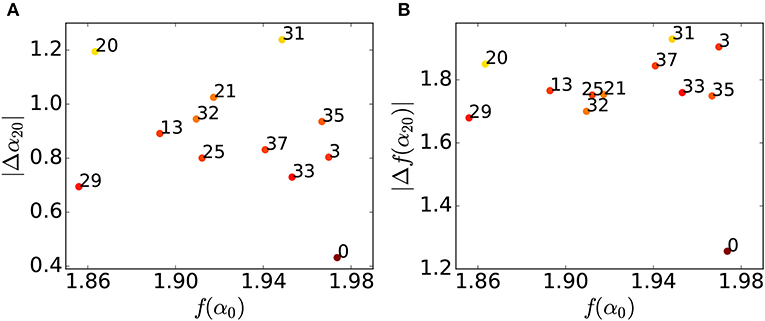
Figure 8. Summary of multifractal properties. (A) The difference between the largest singularity strength α₀ and the smallest one α₂₀, |Δα₂₀|, against the box-counting dimension of the support f(α₀). (B) The difference between the largest spectrum f(α₀) and the smallest one f(α₂₀), |Δf(α₂₀)|, against the box-counting dimension of the support f(α₀). In both panels, the number beside each plot shows the category. The color of each plot represents the value of |ΔD₂₀|. The brighter color corresponds to the larger |ΔD₂₀|.

On the other hand, the vertical axes in Figure 8 show the values that incorporate the differences in the densities in the units. In Figure 8A, the vertical axis shows the difference between the largest and the smallest singularity strength |Δα₂₀|. The color of each marker represents the value of |ΔD₂₀|, for each category. The brighter marker color corresponds to the larger value of |ΔD₂₀|. In Figure 8B, the vertical axis shows the difference between the largest and the smallest spectrum |Δf(α₂₀)|. The color of each marker again represents the value of ΔD₂₀.

The values of |Δα₂₀| and |Δf(α₂₀)| for some categories can diverge even when f(α₀) takes almost the same value. For example, |Δα₂₀| of 29SF is much smaller than that of 20FIN, while f(α₀) of both of these categories are around 1.86. This result indicates that both 29SF and 20FIN have sparse spatial distributions, but the heterogeneity of the densities in the units for 20FIN is stronger than that of 29SF—this can be observed in Figures 2D,G. In Figure 8A, the plots of 3CC and 33HW are nearer that of the population than the others. This suggests that the nature of the spatial distribution in these categories is similar to that of the population when we consider the large region covered by stores/facilities and the small differences in the relative densities in the units.

4. Discussion

In this study, we evaluated whether the spatial distributions of the population and stores/facilities exhibit multifractality. Multifractality in the spatial distribution of the population has been demonstrated in previous studies [3, 5, 10]; we also demonstrated this result in the Kantō area, Japan. However, we were not able to observe multifractality in the population distribution for negative values of q. In the previous studies that evaluated multifractality in city morphologies, the authors carefully examined the range of q in which multifractality was observed [4, 7, 8]. These studies showed that multifractality can be observed at both positive and negative values of q. As we mentioned above, positive (the negative) values of q corresponds to boxes with high (low) densities. Therefore, previous studies observed multifractality in both densely and sparsely distributed regions. However, they also showed asymmetry in the positive and negative ranges of q and discussed the structural differences in dense/sparse regions. In our case, the range of q for multifractality suggests that the sparsely populated region does not have a structure characterized by multifractals, attributable to the geographical characteristics of the examined region in this study. The examined region includes the mountainous areas in the upper and left sides of each panel in Figure 2 as it represents the general feature of the Japanese terrain. It also contains Tokyo bay in the lower-right corner of each panel (Figure 2). Along Tokyo bay, there are rich residential areas as well as plenty of facilities in various industries and numerous stores. This examined region should be an interesting object to investigate considering these geographical features. However, complex substrates may restrict the range in which multifractality appears.

We also investigated which category of stores/facilities shows multifractality for the same ranges of q and ε as that for the population. Stores/facilities in some categories also exhibit multifractality in the spatial distribution, but the determined multifractal measures significantly depend on the category. Diverging multifractal properties can reflect qualitative differences in the spatial distributions—stores/facilities are sparsely and uniformly scattered in some categories, while others are centralized, e.g., the stations in some categories. Importantly, our analysis showed that the box-counting dimension performs poorly in capturing qualitative diversities in the spatial distributions of these categories. The box-counting dimension captures the arrangement of the units that are not empty. On the other hand, multifractal measures can represent the arrangement of units with a certain density. Multifractal curves can indicate, for example, the existence of units with comparably high densities by evaluating the range of the singularity strength α, and the spatial distribution of such units by the spectrum f(α).

The spatial distribution of the population can be characterized by the high box-counting dimension of the support and the homogeneity measured by the generalized dimension and the multifractal curve. The population is distributed across all the regions examined in this study, while the densities in a unit do not vary significantly. In addition, we will observe a similar spatial distribution, even when we change the filter on units according to these densities. Considering its high box-counting dimension and the homogeneity seen in the range of the singularity strength, the spatial distribution of stores/facilities in 33HW exhibits similar features with that of the population. These stores/facilities cover a large area and the heterogeneity of the densities in the units is low. On the other hand, in the cases of 20FIN and 31AED, the singularity strength and the spectrum sharply decline with q. This shape of the multifractal curves indicates a strong centralization of stores/facilities to a few locations. Some of these concentrated locations presumably correspond to large stations in the capital.

In addition to multifractality of the spatial distribution, the scaling law is also a universal pattern observed in city morphology [16–21, 37, 38]. For example, the population X and a quantity Y related to the city morphology have the relationship of Y ~ X^β. The large scaling exponent β in this relationship, i.e., the super-linear increase of Y with X, indicates a strong concentration of these urban-related objects to locations with a large population. Previous studies also found the scaling law in (industrial) agglomerations and showed that facilities, outputs, and jobs concentrated stronger in cities with a large population when these objects are in a category associated with professional and complex skills or with commercial facilities than when the type is relatively primitive or public-related [16, 19–21]. Many of our results are consistent with these previous studies. Our multifractal analysis indicates the centralization of facilities in 20FIN, which is a category related to services requiring professional skills and frequent communication with customers [14]. Also, 31AED, a category related to commercial activities, showed a strong concentration. The concentration of objects related to construction and healthcare was shown to be mild in previous studies, which is also consistent with the mild decline of the singularity strength with q in our results (3CC and 33HW).

While consistency between multifractality and the scaling law exists, an advantage of multifractal analysis should be the richness of information in the result. As we discussed so far, we can quantify the nature of the divergence of the densities in each location and the spatial distribution of each density, by multifractal analysis. For example, for the centralization of stores/facilities in 20FIN and 31AED, multifractal properties further explain the following difference. Considering the large range in the singularity strength and the high box-counting dimension, we can expect to see stores/facilities in 31AED everywhere, with some centralized locations. On the other hand, facilities in 20FIN are encountered only in concentrated locations, which is represented by the overall small singularity strength. Therefore, the results in our analysis exhibit not only the existence of concentrated areas but also the various state of concentration. In this study, we attempted to interpret the multifractal curves that correspond to qualitatively diverging spatial distributions. We hope that our discussion will contribute to future investigations on spatial distributions by multifractal analysis. Additionally, the characteristic of concentration of stores/facilities in each category, which was revealed in this study, should be considered in the actual urban design. For example, the stores/facilities in 31AED is expected to have a tendency to concentrate strongly. Such a tendency of agglomeration should be taken into account in advance when it is required to avoid an extreme concentration of buildings in a landscape.

The temporal development of various urban morphologies, e.g., the spatial distributions of streets and buildings, have been discussed in previous studies [2, 4, 7–9]. Some of them revealed that the spatial distribution was developed to the packed state and to exhibit features close to monofractals [2, 4]. We are also interested in how these developments depend on the category in which the stores/facilities belong. As a future perspective, the comparison of such developments is possible by quantification with multifractal analysis. Furthermore, we expect that the classification of cities is possible by comparing such developments between cities.

Data Availability Statement

The datasets presented in this article are not readily available because these are available under the contract. Requests to access these datasets should be directed to Zenrin Co., Ltd., https://www.zenrin.co.jp/product/category/gis/contents/teldt/index.html for Corporate Telephone Directory Database Telepoint with Coordinates (Telepoint Pack!) and to Zenrin Marketing Solutions Co., Ltd., https://www.zenrin-ms.co.jp/gis_marketing/database/statistics/census_100m_mesh/ for Japanese 100-Meter Estimated Mesh Data of the 2015 National Censuses.

Author Contributions

MI and TO contributed the conception and design of the study, performed the statistical analysis, and wrote the sections of the manuscript. MI wrote the first draft of the manuscript. All authors contributed to the article and approved the submitted version.

Funding

This work was supported by JSPS KAKENHI Grant Number JP16H02872.

Conflict of Interest

The authors declare that the research was conducted in the absence of any commercial or financial relationships that could be construed as a potential conflict of interest.

Acknowledgments

This work was supported by Joint Research Program No. 674 at CSIS, UTokyo [Telepoint Pack DB February 2017 (Yellow pages) by ZENRIN Co. Ltd.].

Supplementary Material

The Supplementary Material for this article can be found online at: https://www.frontiersin.org/articles/10.3389/fphy.2020.00291/full#supplementary-material

References

2. Encarnação S, Gaudiano M, Santos FC, Tenedório JA, Pacheco JM. Fractal cartography of urban areas. Sci Rep. (2012) 2:527. doi: 10.1038/srep00527
3. Appleby S. Multifractal characterization of the distribution pattern of the human population. Geogr Anal. (1996) 28:147–60. doi: 10.1111/j.1538-4632.1996.tb00926.x
4. Murcio R, Masucci AP, Arcaute E, Batty M. Multifractal to monofractal evolution of the London street network. Phys Rev E. (2015) 92:062130. doi: 10.1103/PhysRevE.92.062130
5. Ozik J, Hunt BR, Ott E. Formation of multifractal population patterns from reproductive growth and local resettlement. Phys Rev E. (2005) 72:046213. doi: 10.1103/PhysRevE.72.046213
6. Ariza-Villaverde AB, Jiménez-Hornero FJ, De Ravé EG. Multifractal analysis of axial maps applied to the study of urban morphology. Comput Environ Urban Syst. (2013) 38:1–10. doi: 10.1016/j.compenvurbsys.2012.11.001
7. Chen Y, Wang J. Multifractal characterization of urban form and growth: the case of Beijing. Environ Plann B Plann Des. (2013) 40:884–904. doi: 10.1068/b36155
8. Hu S, Cheng Q, Wang L, Xie S. Multifractal characterization of urban residential land price in space and time. Appl Geogr. (2012) 34:161–70. doi: 10.1016/j.apgeog.2011.10.016
9. Salat H, Murcio R, Yano K, Arcaute E. Uncovering inequality through multifractality of land prices: 1912 and contemporary Kyoto. PLoS ONE. (2018) 13:e0196737. doi: 10.1371/journal.pone.0196737
10. Chen Y, Zhou Y. Multi-fractal measures of city-size distributions based on the three-parameter Zipf model. Chaos Solit Fract. (2004) 22:793–805. doi: 10.1016/j.chaos.2004.02.059
11. Peitgen HO, Jürgens H, Saupe D. Chaos and Fractals: New Frontiers of Science. New York, NY: Springer Science & Business Media (2006).
12. Meakin P. Fractals, Scaling and Growth Far From Equilibrium, Vol. 5. Cambridge: Cambridge University Press (1998).
13. Salat H, Murcio R, Arcaute E. Multifractal methodology. Phys A. (2017) 473:467–87. doi: 10.1016/j.physa.2017.01.041
14. Diodato D, Neffke F, O'Clery N. Why do industries coagglomerate? How Marshallian externalities differ by industry and have evolved over time. J Urban Econ. (2018) 106:1–26. doi: 10.1016/j.jue.2018.05.002
15. O'Clery N, Heroy S, Hulot F, Beguerisse-Diaz M. Unravelling the forces underlying urban industrial agglomeration. arXiv. (2019) 1903.09279.
16. Balland PA, Jara-Figueroa C, Petralia SG, Steijn MP, Rigby DL, Hidalgo CA. Complex economic activities concentrate in large cities. Nat Hum Behav. (2020) 4:248–54. doi: 10.1038/s41562-019-0803-3
18. Bettencourt LM, Lobo J, Helbing D, Kühnert C, West GB. Growth, innovation, scaling, and the pace of life in cities. Proc Natl Acad Sci USA. (2007) 104:7301–6. doi: 10.1073/pnas.0610172104
19. Cottineau C, Hatna E, Arcaute E, Batty M. Diverse cities or the systematic paradox of urban scaling laws. Comput Environ Urban Syst. (2017) 63:80–94. doi: 10.1016/j.compenvurbsys.2016.04.006
20. Um J, Son SW, Lee SI, Jeong H, Kim BJ. Scaling laws between population and facility densities. Proc Natl Acad Sci USA. (2009) 106:14236–40. doi: 10.1073/pnas.0901898106
21. Youn H, Bettencourt LM, Lobo J, Strumsky D, Samaniego H, West GB. Scaling and universality in urban economic diversification. J R Soc Interface. (2016) 13:20150937. doi: 10.1098/rsif.2015.0937
22. Linard C, Gilbert M, Snow RW, Noor AM, Tatem AJ. Population distribution, settlement patterns and accessibility across Africa in 2010. PLoS ONE. (2012) 7:e31743. doi: 10.1371/journal.pone.0031743
23. Scott LM, Janikas MV. Spatial statistics in arcgis. In: Fischer M, Getis A, editors. Handbook of Applied Spatial Analysis. Berlin; Heidelberg: Springer (2010). p. 27–41. doi: 10.1007/978-3-642-03647-7_2
24. Guo D, Zhou H, Zou Y, Yin W, Yu H, Si Y, et al. Geographical analysis of the distribution and spread of human rabies in china from 2005 to 2011. PLoS ONE. (2013) 8:e72352. doi: 10.1371/journal.pone.0072352
25. Carlow G, Zinke-Allmang M. Self-similar spatial ordering of clusters on surfaces during Ostwald ripening. Phys Rev Lett. (1997) 78:4601. doi: 10.1103/PhysRevLett.78.4601
26. Riitters K. Pattern metrics for a transdisciplinary landscape ecology. Landsc Ecol. (2019) 34:2057–63. doi: 10.1007/s10980-018-0755-4
27. Saeki K, Sasaki A. The role of spatial heterogeneity in the evolution of local and global infections of viruses. PLoS Comput Biol. (2018) 14:e1005952. doi: 10.1371/journal.pcbi.1005952
28. Ellison G, Glaeser EL, Kerr WR. What causes industry agglomeration? Evidence from coagglomeration patterns. Am Econ Rev. (2010) 100:1195–213. doi: 10.1257/aer.100.3.1195
29. Jiang ZQ, Xie WJ, Zhou WX, Sornette D. Multifractal analysis of financial markets: a review. Rep Prog Phys. (2019) 82:125901. doi: 10.1088/1361-6633/ab42fb
30. Stanley HE, Meakin P. Multifractal phenomena in physics and chemistry. Nature. (1988) 335:405–9. doi: 10.1038/335405a0
31. Saa A, Gascó G, Grau J, Antón J, Tarquis A. Comparison of gliding box and box-counting methods in river network analysis. Nonlin Process Geophys. (2007) 14:603–13. doi: 10.5194/npg-14-603-2007
32. Sun X, Chen H, Wu Z, Yuan Y. Multifractal analysis of Hang Seng index in Hong Kong stock market. Phys A. (2001) 291:553–62. doi: 10.1016/S0378-4371(00)00606-3
33. Torre I, Losada JC, Heck R, Tarquis A. Multifractal analysis of 3D images of tillage soil. Geoderma. (2018) 311:167–74. doi: 10.1016/j.geoderma.2017.02.013
34. Grau J, Méndez V, Tarquis AM, Diaz MC, Saa A. Comparison of gliding box and box-counting methods in soil image analysis. Geoderma. (2006) 134:349–59. doi: 10.1016/j.geoderma.2006.03.009
35. Chhabra A, Jensen RV. Direct determination of the f (α) singularity spectrum. Phys Rev Lett. (1989) 62:1327–30. doi: 10.1103/PhysRevLett.62.1327
36. Chhabra AB, Meneveau C, Jensen RV, Sreenivasan K. Direct determination of the f (α) singularity spectrum and its application to fully developed turbulence. Phys Rev A. (1989) 40:5284–94. doi: 10.1103/PhysRevA.40.5284
37. Nomaler Ö, Frenken K, Heimeriks G. On scaling of scientific knowledge production in us metropolitan areas. PLoS ONE. (2014) 9:e110805. doi: 10.1371/journal.pone.0110805
Keywords: multifractal analysis, spatial distribution, population, stores/facilities, agglomeration
Citation: Ito MI and Ohnishi T (2020) Evaluation of the Heterogeneous Spatial Distribution of Population and Stores/Facilities by Multifractal Analysis. Front. Phys. 8:291. doi: 10.3389/fphy.2020.00291
Received: 14 April 2020; Accepted: 26 June 2020;
Published: 04 August 2020.
Edited by:
Gabjin Oh, Chosun University, South KoreaReviewed by:
Gui-Quan Sun, North University of China, ChinaJiuchuan Jiang, Nanjing University of Finance and Economics, China
Copyright © 2020 Ito and Ohnishi. This is an open-access article distributed under the terms of the Creative Commons Attribution License (CC BY). The use, distribution or reproduction in other forums is permitted, provided the original author(s) and the copyright owner(s) are credited and that the original publication in this journal is cited, in accordance with accepted academic practice. No use, distribution or reproduction is permitted which does not comply with these terms.
*Correspondence: Mariko I. Ito, marikoito.rnu1@gmail.com