Using ecological partitions to assess zooplankton biogeography and seasonality

1 Introduction

Zooplankton perform key ecosystem services and are a critical component of biogeochemical fluxes in the pelagic ocean. They are the primary vectors in the transfer of organic carbon produced by phytoplankton from the uptake of CO₂ to higher trophic levels (Marquis et al., 2011) and play an important role in biogeochemical cycles, regulating carbon sequestration in the deep ocean as part of the biological carbon pump. They do this in a number of ways from the passive sinking of organic detritus and faecal pellets (Turner, 2015), fragmenting sinking particles through grazing (Cavan et al., 2017), and through the active daily migrations (Steinberg et al., 2000; Archibald et al., 2019) or seasonal deep-ocean overwintering in higher latitudes (Jónasdóttir et al., 2015). Limited availability of suitable data and complexity within zooplankton communities has made parameterization of key processes performed by this group particularly challenging to include in biogeochemical models (Giering et al., 2019).

Marine biogeochemical models describe the flow of elements between the biogeochemical compartments, such as Nutrients, Phytoplankton, Zooplankton and Detritus (NPZD, Edwards, 2001). Model evolution is determined by differential equations that parameterize the controls on phytoplankton growth (e.g. nutrient, light), zooplankton grazing, plankton mortality, and remineralization of organic matter back to inorganic nutrients. In most current global scale biogeochemical models, zooplankton are the highest trophic level explicitly modelled and as a result they are key in limiting blooms of phytoplankton and their parameterization is important for the rate of production of detritus (Steele and Henderson, 1992) and export of carbon. Historically, zooplankton has often been the poorest performing group when validating models with in situ data (Arhonditsis and Brett, 2004). Zooplankton parameterization and estimates likely suffer more than phytoplankton due to the enhanced complexity of their behavior and life history strategies. The productivity and diversity estimated by models are quite different depending on the specific rates and type of parameterization chosen for the zooplankton (see e.g. Vallina et al., 2014; Prowe et al., 2012; Chenillat et al., 2021; Karakuş et al., 2022). However, there has in general been a lack of data with which to ascertain which of several model outcomes of zooplankton biomass is most plausible.

Evaluating zooplankton performance within biogeochemical models is difficult due to the mismatch between the regular gridded output of a model and the irregular sampling distribution and methodologies of zooplankton observations (Everett et al., 2017). The number of zooplankton sampling nets or devices available are manifold, each with their own specific trade-offs in sampling and operational efficiency. These vary across the traditional vertical or obliquely towed nets (e.g. – WP2), multi-nets for depth stratified sampling (e.g. – MOCNESS, Wiebe et al., 1985) and highspeed samplers (e.g. – CPR, Richardson et al., 2006). In addition, mesh sizes will also vary in accordance with the sampling area or target groups (Sameoto et al., 2000). To produce a reliable database of zooplankton biomass, a significant amount of quality control and standardization is needed before any comparison between model and data can take place (Moriarty and O’Brien, 2013). Even with the collation of global zooplankton datasets there is a large disparity in the spatial coverage of measurements in the ocean with over 81% of observations in temperate latitudes of the northern hemisphere (Ratnarajah et al., 2023). Aggregating these data onto an appropriate grid and temporal scale to match the biogeochemical model will result in large swathes of the ocean with little or no coverage.

There is a critical need to develop and test models of zooplankton biomass dynamics in our oceans (Everett et al., 2017). Here, we develops a method that addresses the two primary issues that are encountered when assessing the model performance of zooplankton in biogeochemical models. The first stage deals with standardizing the available zooplankton observations by converting abundance and biomass measurements from different platforms and net types into comparable units. The second stage deals with the spatial component where the gridded model and irregularly sampled field data are combined by partitioning the ocean into regions defined by a set of biotic and abiotic conditions. One of the most commonly used partitions is the Longhurst Biogeochemical Provinces (Longhurst, 2007) which used key biogeochemical parameters to delineate the main oceanographic regions. Global-scale satellite data and biological databases have allowed for partitioning of the ocean to be driven by objective classifications based on physical, chemical, or biological data (i.e., temperature and ocean color, Oliver and Irwin, 2008; community composition, Beaugrand et al., 2019; Elizondo et al., 2021).

We develop an ocean partition framework to facilitate the assessment of zooplankton model output with our standardized zooplankton observations. We use output from the MIT Darwin biogeochemical-ecosystem model (Dutkiewicz et al., 2015) which predicts zooplankton biomass fluctuations globally. We partition the ocean by identifying areas where the seasonal cycle varies consistently and distinctly compared to other areas. Differences in phenology, frequency and magnitude of zooplankton biomass fluctuations over a year are used to partition the ocean. We use data collected in-situ many research cruises and net types. Data come largely in the form of biomass and volumetric measurements of zooplankton which are standardized to a common metric of biomass to be compared with the model output. Our method for partitioning of the ocean is designed to address the challenge of data sparsity in data-model comparisons

2 Methods

We used output from the MIT Darwin model (Dutkiewicz et al., 2015) as an illustration of our method. We gathered a large collection of field observations of zooplankton and standardized observations to the same biomass units. Given the sparsity of the data, we addressed model skill not point to point, but within partitions. Partition were defined based on seasonality of the modelled zooplankton biomass. The modelled and in-situ zooplankton biomass measurements were aggregated within each partition and time intervals to create two time series to enable comparison of their average seasonal dynamics. We propose and test several assessments that allow for temporal and geographic mismatch between data and model to be quantified at the global scale.

2.1 Zooplankton observations

Global mesozooplankton biomass data were extracted from the Coastal and Oceanic Plankton Ecology, Production, and Observation Database (COPEPOD, O’Brien, 2007) and the Continuous Plankton Recorder (CPR, Richardson et al., 2006). COPEPOD is repository of zooplankton biomass data derived from sampling programs and individual cruises with the earliest collected in 1932. Sample availability increased significantly in the 1950’s and remained relatively consistent over time (Figure 1). The CPR is the largest marine survey in the world having sampled near surface (~10 m) plankton behind ships of opportunity across 7 million nautical miles of ocean since 1931, though our earliest samples were collected in 1948. While much of the data comes from the North Atlantic, the survey has expanded through the development of sister surveys to other areas including the North Pacific (Batten et al., 2006) and the Southern Ocean (Hosie et al., 2003). As a result, we see an increase in the number of CPR observations over the last 20 years (Figure 1). A wide array of different methodologies has been used to quantify total zooplankton biomass in the COPEPOD database including accounting for different mesh sizes, depths sampled and biomass calculation (e.g. – settled volume, dry weight etc.). We followed the two-step approach outlined in Moriarty and O’Brien (2013) beginning by converting observations to carbon mass (g C m^-3) (Supplementary Table 1). The second step standardizes observations collected with many different mesh sizes to approximate a 333 µm mesh equivalent using conversion equations developed by O’Brien (2005) (Supplementary Table 1). COPEPOD includes both vertical net tows and stratified sampling at different depths. We restricted our samples to those collected in the upper 100 m (Figure 1; n = 209, 688). CPR data are represented as species abundances which require a conversion to dry weight of an individual using length – weight regression equations (see Supplementary Tables 1, 2 for length measurements used) which are then converted to carbon mass (Figure 1; n = 264, 512) (Figure 2A). While the CPR mesh size (270 µm) differs from the 333 µm mesh equivalent, we were unable to perform the same mesh size standardization due to the lack of direct time and date matches in both datasets. We studied the consequence of combining both datasets in areas where both COPEPOD and CPR data were collected through analyses of each dataset separately and combined.

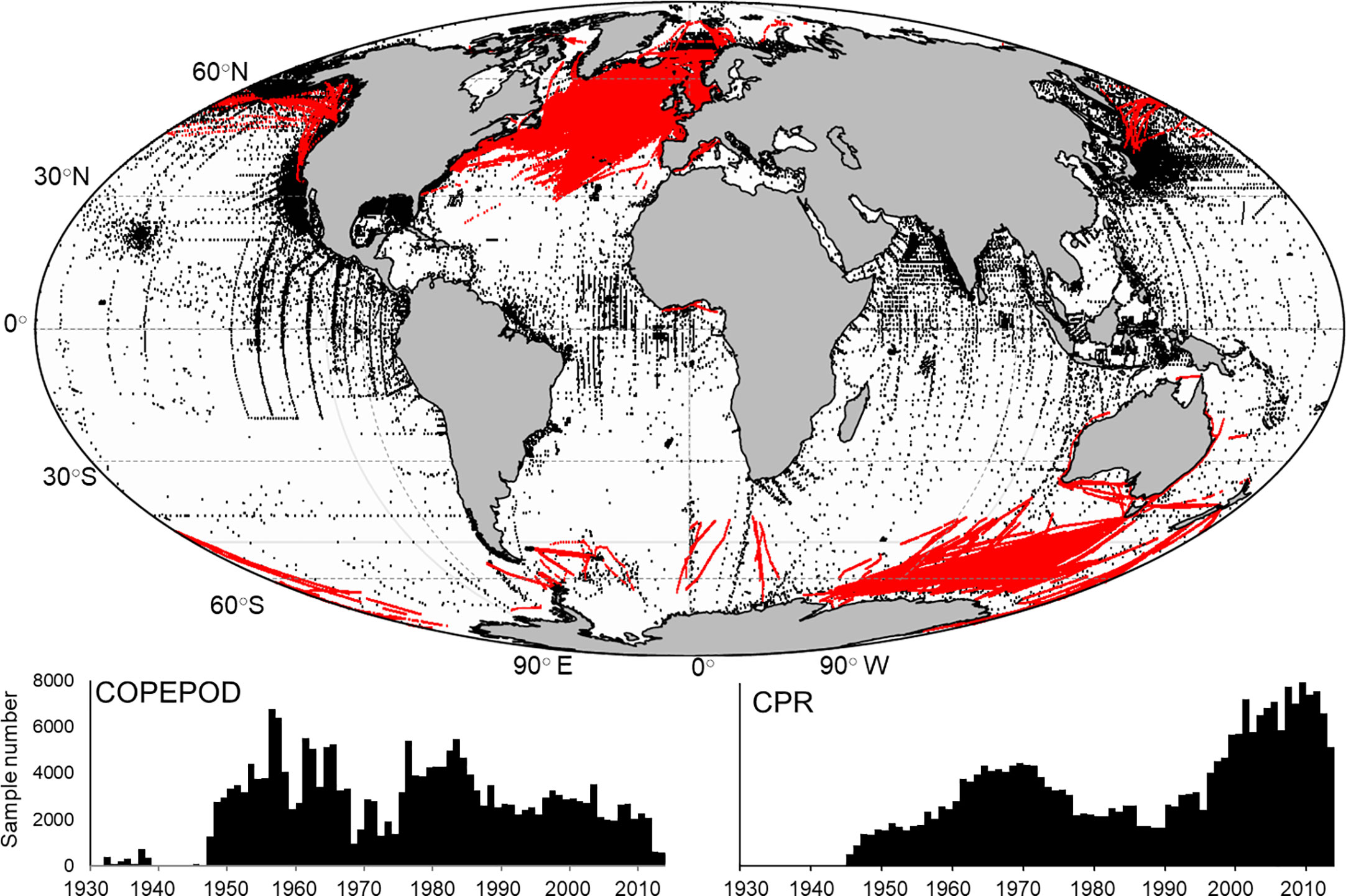
Figure 1 (top) The global distribution of surface (0-100 m) mesozooplankton biomass measurements from the COPEPOD database (black dots; n = 209,688) and samples taken from the Continuous Plankton Recorder (red dots; n = 264,512). Also shown is the sample frequency for each year for both the COPEPOD (bottom left) and CPR (bottom right) databases.

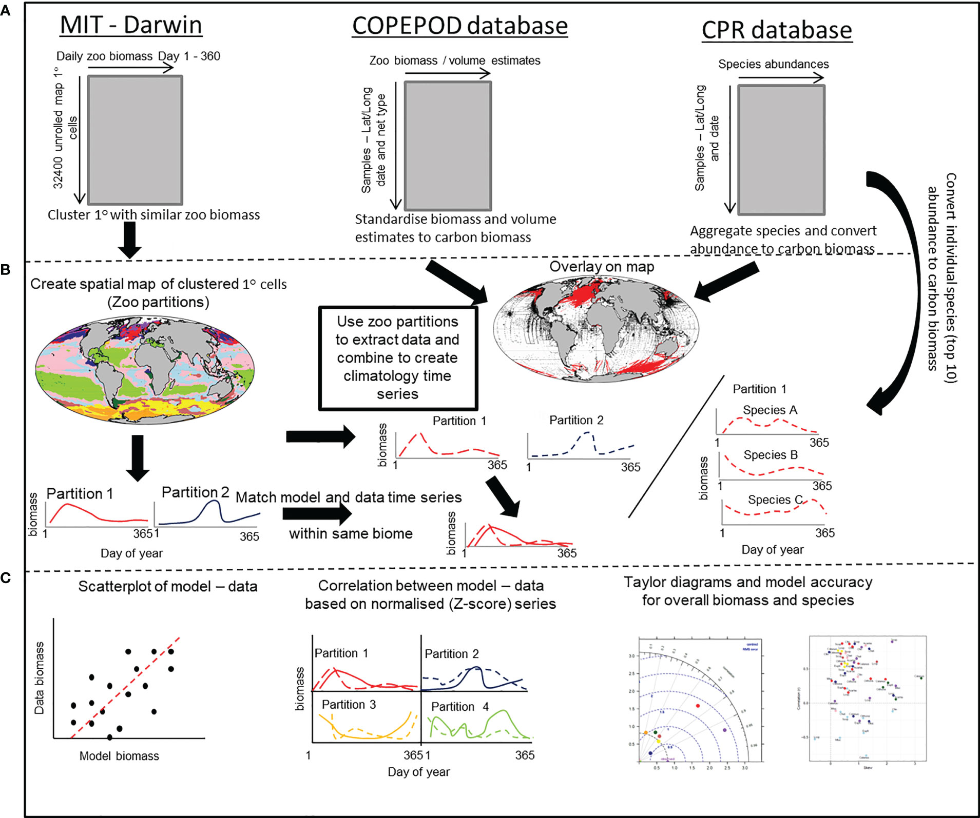
Figure 2 A schematic that outlines the stepwise procedure for comparing modelled and in-situ mesozooplankton carbon biomass. (A) Shows the structure of the MIT-Darwin model data and the COPEPOD and CPR database that contain the in-situ biomass and count data. (B) The MIT-Darwin data are clustered into regions with similar characteristics of zooplankton annual cycle. Both COPEPOD and CPR database data are standardized to the same metric of carbon biomass derived from MIT-Darwin. The partitions are used to extract data and are averaged within each partition to create a time series of in-situ data that matches the model data estimated within each partition. A similar process is performed for the most abundant (Top 10) species found within the CPR database and treated in the same way. (C) The model and in-situ time series within each of the partitions are compared and contrasted by using a simple scatterplot, correlation of normalized data and taylor diagrams to assess model accuracy. For the individual species, only the correlation and model accuracy is used.

2.2 Modelled zooplankton

Modelled zooplankton biomass (mg C m^–3) was obtained from the MIT Darwin biogeochemical-ecosystem model (Dutkiewicz et al., 2015). The model characterizes the cycling of carbon, nitrogen, phosphorous, silica, iron and oxygen through a system of organic (phytoplankton, zooplankton, detritus) and inorganic pools. The model parameterized the different pools in terms of concentration, and as such plankton are tracked in terms of carbon biomass (mg C m^–3). The movement and mixing of the biological and chemical tracers were driven by the MIT general circulation model. In this version of the model, zooplankton were resolved to two generalized size classes (large and small) that prey preferentially on different phytoplankton classes within the model. We selected the large zooplankton to represent the mesozooplankton biomass range (> 200 µm) due to their preference within the model for diatoms and other large-bodied phytoplankton (Dutkiewicz et al., 2015). The model was run for 10 years with physics from a generic year. After about 3 years a stable seasonally varying ecosystem was established. As in Dutkiewicz et al. (2015) we use output from the 10th year of the simulation. We used averaged surface (0-100 m) daily means of the large zooplankton carbon mass on a global 1x1° grid (Figure 2A).

2.3 Dividing the ocean into zooplankton partitions

Although our partitions are analogous to the global scale partitioning suggested by Longhurst (2007) or ecoregions (Spalding et al., 2007), they do not adhere to these definitions. We classify our regions as zooplankton partitions defined as areas where the zooplankton model output is relatively spatially homogeneous. Global partitions were defined using the 1° cell daily estimates of surface zooplankton using MIT Darwin model carbon mass (MOD_CM). We created a MOD_CM matrix where each row represents the biomass data for each 1° cell and each column represents one of the 365 daily time steps. We defined the number of clusters using k-means clustering. K-means is an unsupervised clustering algorithm that partitions observations into a pre-defined number of clusters k by minimizing the error sum of squares (ESS) within each cluster. The optimum number of clusters k is found following the procedure outlined by McGinty et al. (2011). Briefly, the optimum k is found through an iterative process where the explained variance is computed for increasing values of k. The explained variance grows logistically with increasing k and the optimum number of clusters was identified when the step-wise increase in explained variance fell to less than 5% of the maximum increase observed.

The partitions were used to aggregate the total carbon mass from both COPEPOD and CPR observations (DAT_CM), creating a time series representing the average seasonal pattern of measured zooplankton biomass within each partition. The carbon mass data from COPEPOD and CPR were combined and averaged into 36, 10-day climatological bins (DAT_CM) within each partition. Time-series were also prepared for the 5 most abundant taxonomic groups from each CPR survey (CPR_CM, see Supplementary Table 1). Partition-wide daily mean values of MOD_CM were calculated and further averaged across each 10-day period to match the temporal resolution of the DAT_CM and CPR_CM (Figure 2B).

2.4 Model – data comparison metrics

Quantitative model assessment of the MOD_CM was performed using commonly used statistical and graphical methods namely: scatterplots, Taylor diagrams and skewness. Scatterplots are a valuable diagnostic tool in model evaluation. They can be used to visualize the relationships between MOD_CM and DAT_CM and a least squares regression analysis was used to assess the strength of these relationships. A regression with a slope 1 and intercept 0 indicates a perfect match between model and data. Taylor diagrams (Taylor, 2001) were used to summarizes relationships between observed data and model output by simultaneously displaying the Pearson correlation (r), standard deviation of DAT_CM - MOD_CM (SD) and root mean square error (RMSE). The diagram displays the correlation strength along the azimuth angle, the SD is displayed radially from the origin and the RMSE is proportional to the observed reference along the x-axis where the correlation is equal to 1. Skewness is a measure of the asymmetry of the error distribution (observations – model) about its mean. A positive skew indicates that the error distribution has an asymmetric tail towards large positive values (model underestimation) and in contrast a negative skew indicates that the error distribution has an asymmetric tail towards more negative values (model overestimation). Skewness values of 2 or more were considered notable. Assuming data were available for all 36-time intervals, a skewness larger than 0.4 in magnitude was judged as significantly skewed (Figure 2C).

Data were normalized to a mean of zero and a standard deviation of 1 to produce a dimensionless z-score for both MOD_CM and DAT_CM in each partition. This allowed for a qualitative comparison of the spatial and temporal differences between the model and observational across the year. Cross-correlations were used to assess whether the relationship could be improved by assessing lagged process between model and observational data within each partitions. An improvement in correlation between model and data with a positive time lag indicated that the model reported later peaks in biomass compared with observational data while a negative time lag indicated the model reported earlier peaks in biomass compared with observational data (Figure 2C).

To assess the effect of combining the COPEPOD and CPR database we correlated each database with the MOD_CM in each partition where both datasets were collected and compared these results with the correlations obtained using DAT_CM. DAT_CM was preferred if there was an overall increase in the correlation of model and observations using DAT_CM compared with using each database separately (Supplementary Figure 1).

3 Results

3.1 Zooplankton partition classification

An optimum number of 10 zooplankton partitions were defined with a total R² of 75.5% (Figure 3). Despite the unsupervised nature of k-means clustering and that the clustering did not incorporate geographic information, the partitioning had significant spatial coherence. The partitions in the higher latitudes (poleward of 40^○) of both hemispheres were separated along a latitudinal gradient with partition A, I and J representing polar/sub polar ecosystems. Temperate ecosystems were represented by partition B in the northern hemisphere and H in the southern hemisphere. Within the sub-tropical and tropical ocean we found that the clusters were defined less by latitude than by the position of the large oceanic gyres and ocean currents. For example, partition F encompassed much of the oligotrophic gyres in the open ocean, particularly in the southern hemisphere while partitions D and E defined the transition zones, particularly across the North Pacific and within the Indian Ocean. Partitions C and G were patchier in distribution and hugged the continental coastline in areas of known upwelling or downwelling. Partition C appeared almost exclusively in the northern hemisphere while partition G occurred most often in the southern hemisphere.

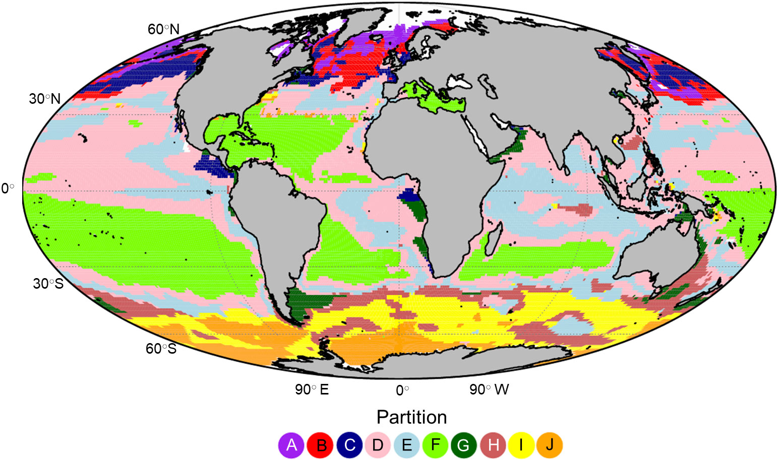
Figure 3 The global projection of the 10 global zooplankton partitions labelled (A-J) which were defined using k-means clustering on the large zooplankton biomass measurements derived from the Darwin model.

3.2 Model – data comparison

Overall, there was a significant positive relationship between model and data estimates of mesozooplankton carbon mass (r^{2 =} 0.4, p < 0.001) (Figure 3). The model tended to match observations when the carbon mass was low and underestimated observations at the highest biomass levels with a slope less than 1 (0.62) and a positive offset of 1.76 mg C m^-3 (Table 1). There were differences in the model-data zooplankton biomass relationship across the 10partitions. Partitions D-F and J showed the lowest agreement between model and data with a negative relationship observed between model and data (Figure 4; Table 1). The remaining partitions all showed a significant positive relationship between model and data with the slopes of partitions H (0.76) and I (1.2) closest to 1 (Figure 3; Table 1). Model skill statistics were summarized by the Taylor diagram (Figure 5) and reflect the findings observed with the scatterplots. The tropical partitions (D-F) did not appear on the diagram as the correlation coefficient is close to or less than 0. Except for partition J, the remaining 6 areas all had a significant positive correlation between model and data ranging from 0.42 (G) to 0.92 (A). Both partition B and G had standardized deviations greater than 2 while the remaining partitions are closer to 1.

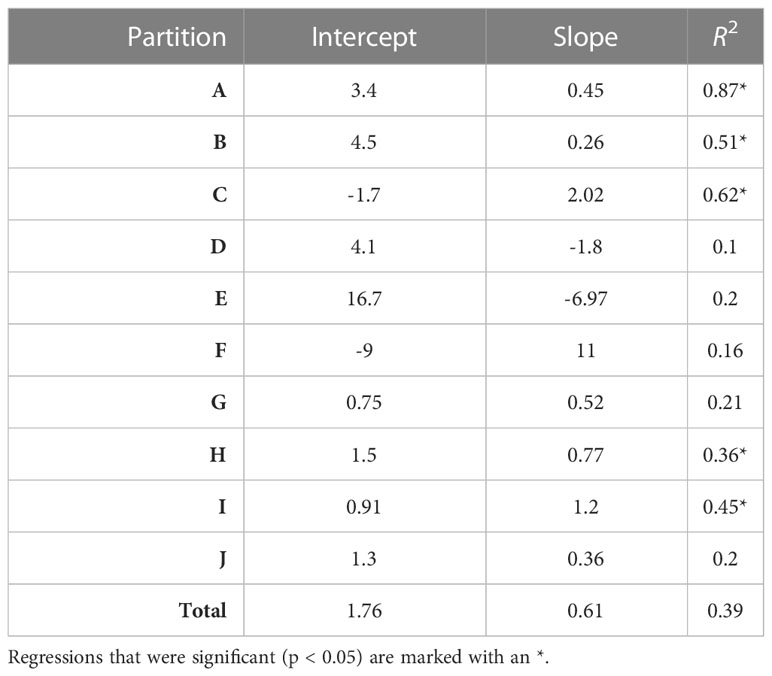
Table 1 The intercept, slope and variance explained (R²) for each linear regression comparing observed and modelled zooplankton biomass (DAT_CM against MOD_CM) within each partition (n=36) and total (n=360).

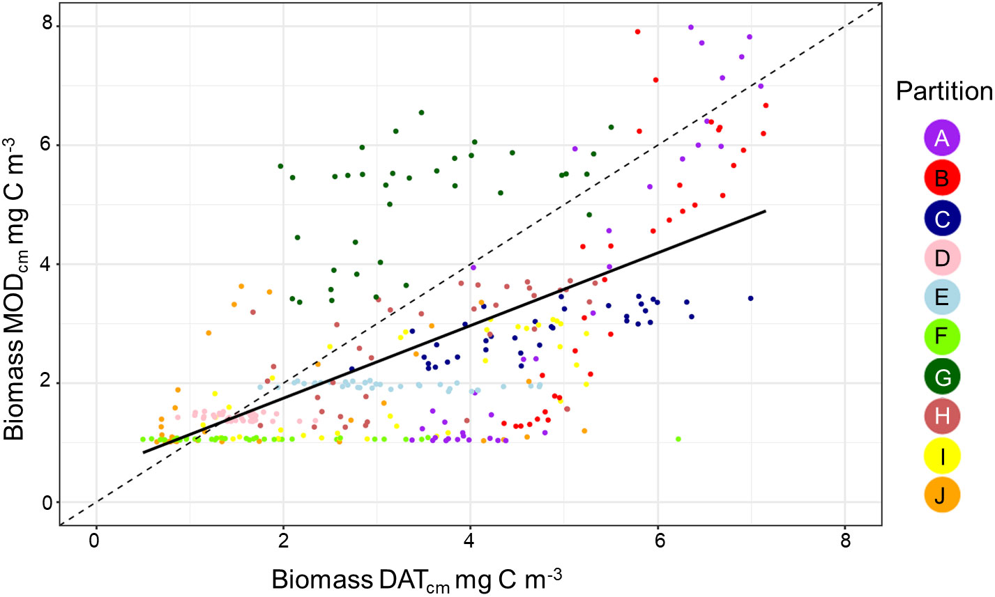
Figure 4 A scatterplot showing the relationship between the in situ data and model biomass. Each point shows the pairwise comparison between data and model for each of the 36 10 day periods within the 10 zooplankton partitions.

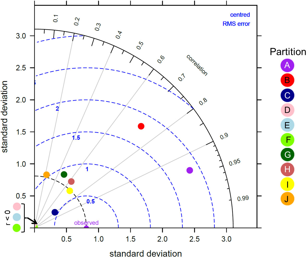
Figure 5 Taylor diagram showing the correlation, normalised standard deviation and root mean square error between the modelled zooplankton biomass from MIT Darwin model and the in situ zooplankton biomass for each of the 10 global zooplankton partitions. A perfect match between model and data is represented by the “observed” point along the correlation of 1 axis.

The normalized biomass plots showed the mean change in the seasonal trends of MOD_CM and DAT_CM within each partition (Figure 6). In general those partitions with a notable bloom cycle displayed the strongest direct correlation between model and data with no temporal lags. There were improvements in the correlation between model and data for half of the partitions with the model lagging 30 days (F and I), 50 days (J) and 120 days (D and E) behind the data (Figure 6). Comparing the correlations between data and model with the skewness of the error distribution show that the temperate and sub-polar partitions A, C, I and H were significantly correlated with skewness close to zero (Figure 7). Only partition B showed a significant negative skewness in the error distribution (model overestimation) with the remaining partitions all showing a significant positive skewness (model underestimation). With the exception of the Antarctic partition J, partitions with a higher sea- surface temperature was less strongly correlated and had a larger model underestimation. The mean SST for the five partitions with a r > 0.5 was 7.8°C while the remaining five partitions were almost 10°C warmer with a mean SST of 17.5°C.

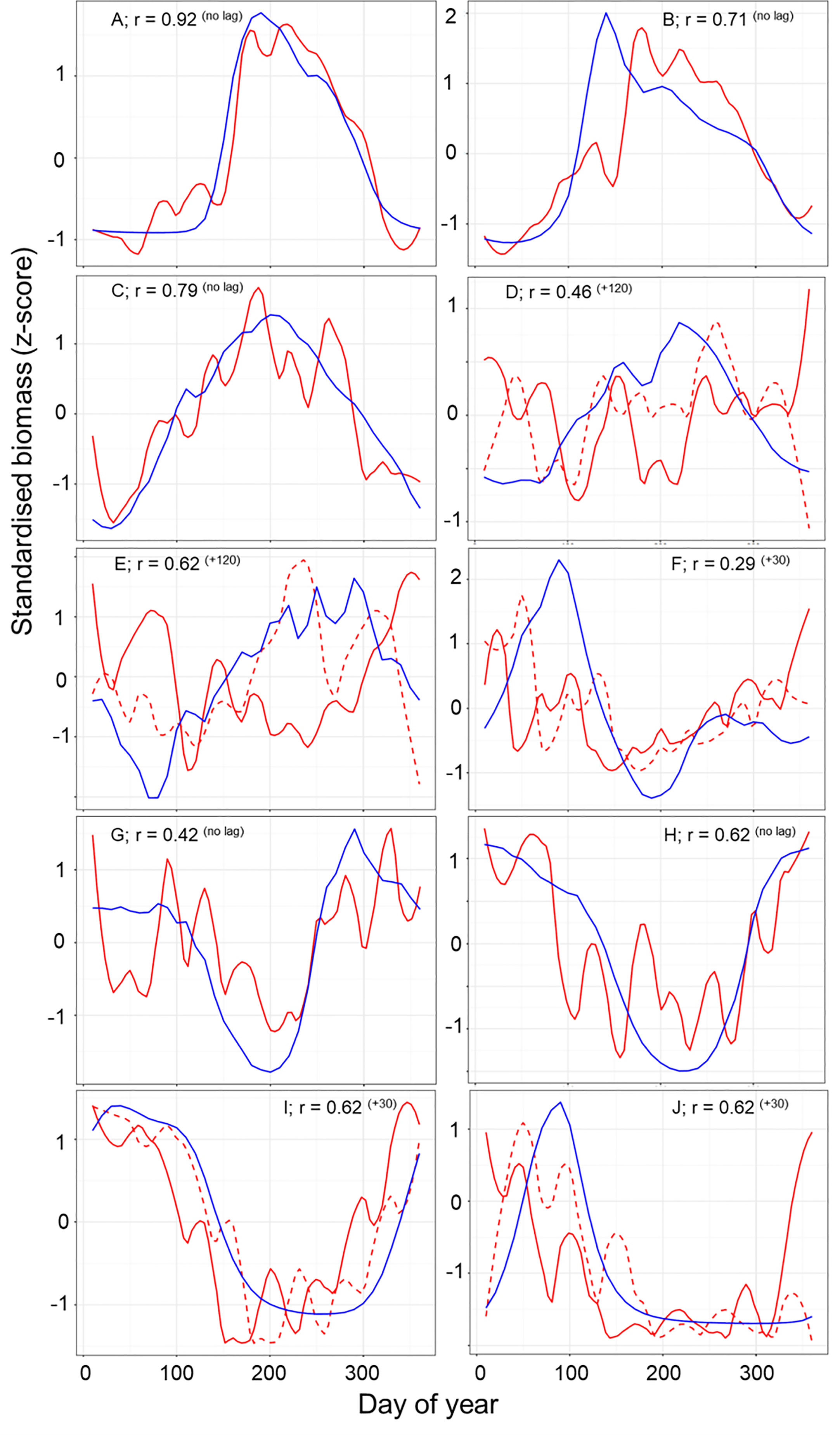
Figure 6 A comparison of the normalized seasonal trend for zooplankton data (red line) and model output (blue line) across the full year. Lagged zooplankton data (dashed red line) time series are shown where lagged data improve correlation between model and data. Each panel shows the strongest Pearson correlation (r) between data and model within each of the 10 zooplankton partitions after accounting for temporal lags r ^(lag). A positive lag indicates that the model trend is shifted later than the data.

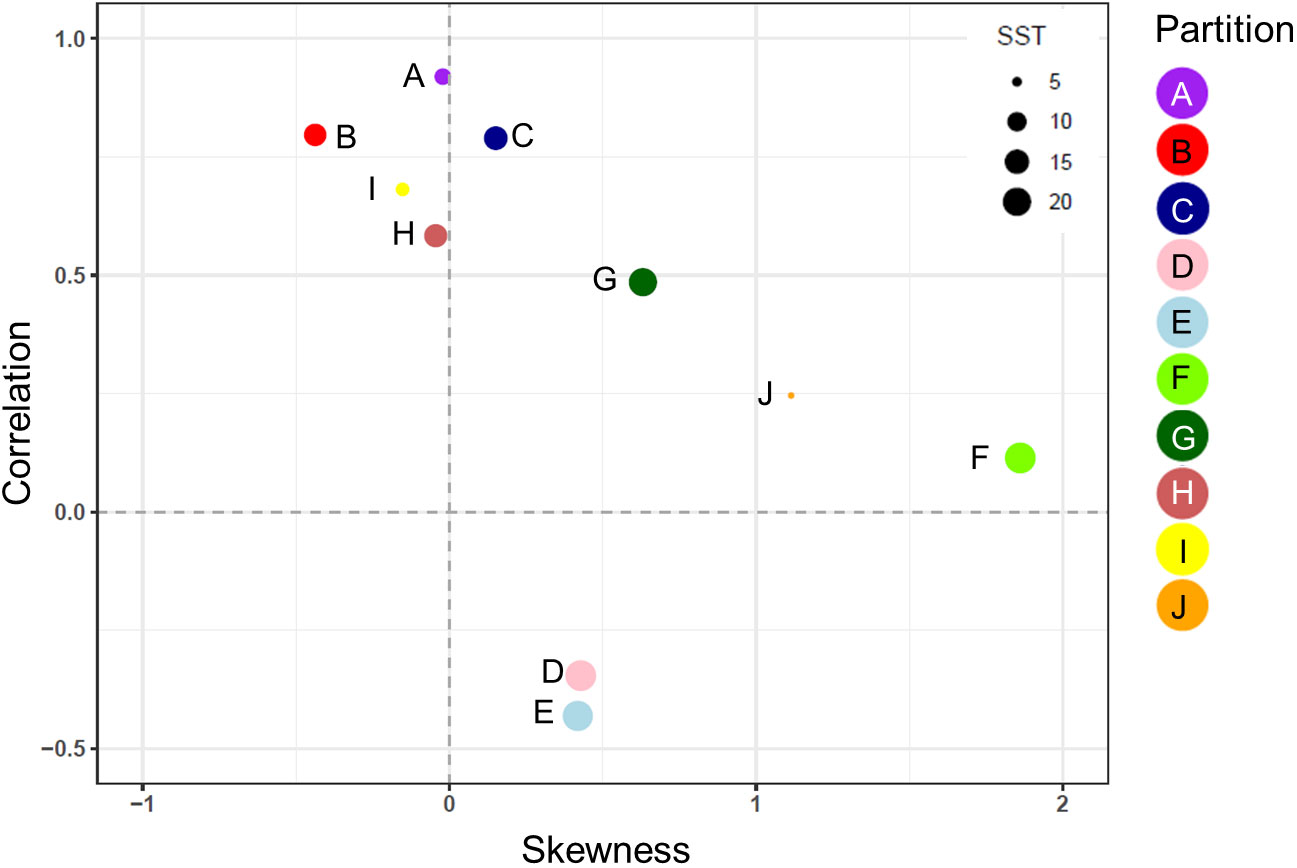
Figure 7 The correlation coefficient (r) and the skewness of the model error distribution between model and in situ data for each of the 10 zooplankton partitions. Positive skew values indicate an error distribution towards model underestimation and vice versa. Each partition cluster is represented by a different color and are scaled according to the mean sea surface temperature (SST) within each partition.

The correlation and skewness were also calculated for 8 partitions with CPR data, comparing the most abundant taxonomic groups with the model carbon mass (Figure 8). In almost all cases there was a positive skewness in the error distribution between the CPR biomass for selected taxa and MOD_CM. Calanus finmarchicus (Cfin) in partition C was the only taxonomic group with a significant correlation and skewness less than 0.4, although a total of 20 taxa among 6 different partitions had significant correlation with varying degrees of positive skew. While some partitions (e.g. G and I) had a similar correlation and skewness among all species within that group, there were other partitions including C that showed significant variation in correlation and skew across species (e.g. Cfin and Metridia lucens – Mluc) (Figure 8).

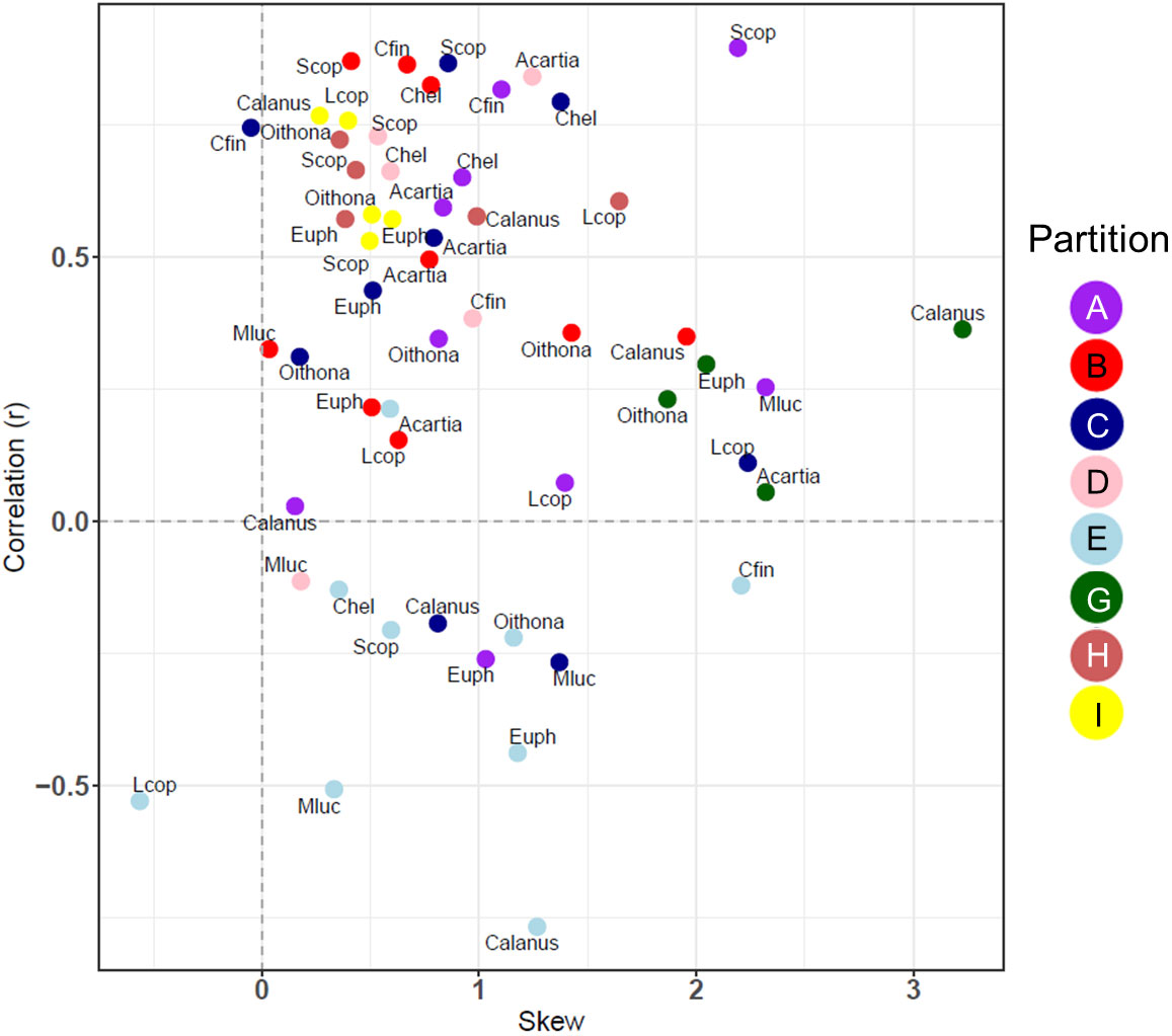
Figure 8 The correlation coefficient (r) and the skewness of the model error distribution between model and in situ species level data for 8/10 of the zooplankton partitions. Positive skew values indicate an error distribution towards model underestimation and vice versa. Each partition cluster is represented by a different color and are labelled with an abbreviation for each species or species. Calanus, Calanus spp.; Oithona, Oithona spp.; Acartia, Acartia spp.; Mluc, Metridia lucens; Chel, Calanus helgolandicus; Cfin, C. finmarchicus; Euph, Euphausiacea; Scop, small copepods; Lcop, Large copepods.

3.3 CPR and COPEPOD comparison

A total of 8 partitions were used to compare the effects of combining measures of carbon mass from COPEPOD and CPR databases (CPR data were not present in partitions F and J). There was a significant improvement in the mean correlation of model and observations across the 8 partitions using DAT_CM (r = 0.55, SE ± 0.12) compared with using COPEPOD (r = 0.33, SE ± 0.09) or CPR (r = 0.44, SE ± 0.09) data only. The CPR had the strongest positive correlation with the model in partitions A (0.67) and C (0.64) while COPEPOD had the strongest correlation with the model in partition I (0.83). A linear regression of observation-model correlation coefficients between DAT_CM and each of the databases showed a significant positive relationship in both COPEPOD (R^{2 =} 0.8; y=1.1x+0.21) and CPR (R^{2 =} 0.58; y=1.16x+0.04). In some partitions the correlation between the CPR and COPEPOD biomass data were negative, such as in partition E (-0.66). The correlations between CPR and COPEPOD databases were strongest in partitions where the observation-model correlation was strongest for DAT_CM (R^{2 =} 0.44; y=0.55x+0.5) (Supplementary Figure 1)

4 Discussion

We have developed a framework to compared sparse observational data with gridded model output by developing ecological partitions based on the seasonal patterns of mesozooplankton carbon mass. Here we used output from the MIT Darwin model (Dutkiewicz et al., 2015), but this framework could be used for skill assessment of any model that includes a mesozooplankton specific output variable. We used the model output to create a global mosaic of partitions defined by the seasonality of the zooplankton. By aggregating data within each partition we compared modelled and observed biomass despite the challenge of irregular and sparse sampling of zooplankton. Model estimates of mesozooplankton carbon mass correlated with observational measurements of zooplankton carbon mass but the model skill varies across each zooplankton partition. The best- performing partitions were in the temperate and sub-polar latitudes (partitions A, B, C, H and I) where the correlations between model and data were greater 0.5 (Figures 3, 4). These regions have strong bloom cycles, which the model was able to capture with relative skill. Except for partition A (which showed significant model overestimation), there was no significant model over- or under-estimation of carbon mass based on the error skewness. Our analysis provides an encouraging assessment of the model performance for zooplankton. The remaining partitions were situated in the equatorial and high polar latitudes and performed poorly in comparison. All correlations in these partitions were less than 0.5 with significant model underestimation based on the error skewness.

The differences in model performance between the temperate/sub-polar and tropical/sub-tropical partitions were likely driven by the magnitude of the seasonal changes in mesozooplankton biomass and the complexity of the trophic pathways. Seasonal biomass can vary by a factor of 20 (Mackas et al., 2007) in the temperate/sub-polar regions but in the tropics the variation may be as low as 2 or 3 (Fernández-Álamo et al., 2006). There is a distinct functional relationship between zooplankton biomass and phytoplankton productivity in the higher latitudes. Areas with a high biomass of large phytoplankton cells (> 20 µm) are more likely to support a more direct trophic pathway to meso-zooplankton which are dominated by herbivores-omnivores (Décima 2022). With larger phytoplankton dominating the spring bloom production there is a much more direct coupling and efficient transfer of carbon between phytoplankton and zooplankton (Cushing, 1989; Romero-Romero et al., 2019). In the tropics and equatorial regions the trophic pathways are often longer and dominated by carnivory which is more difficult to predict (Décima 2022) and was not included in this version of the Darwin model. There are also differences in the inter-annual environmental drivers of phytoplankton and zooplankton growth. In the northern latitudes the springs bloom is an annual event initiated when nutrient and light levels allow for a net- positive growth in phytoplankton with zooplankton following a similar process of rapid population growth. In contrast, the seasonal changes are not as apparent in the tropical oceans with smaller increases and decreases in standing stock driven by regional weather patterns and water mass movement (Fernández-Álamo et al., 2006). Throughout the tropical and sub-tropical ocean much of the surface waters are chronically nutrient depleted with a strong dominance of smaller picophytoplankton species which are not readily consumed by mesozooplankton groups but are instead grazed by smaller protists (Sherr and Sherr, 2002; Schmoker et al., 2013) developing the “microbial loop” (Azam et al., 1983; Passow et al., 2007). In this process grazing in the microbial loop is predominantly driven by microzooplankton (Calbet, 2008; Fenchel, 2008) which are in turn more heavily grazed by the smaller sized carnivorous mesozooplankton species. Grazing measurements at the equator have shown that 83% of phytoplankton production is removed by microzooplankton compared with only 10% of mesozooplankton (Landry et al., 1995). In these regions with more complexity and less seasonality the MIT Darwin model (Dutkiewicz et al., 2015) did not perform well. In the model it is the small zooplankton, which are not compared here due to lack of observational data from these smaller size classes, that presumably dominate the grazing.

In order to improve model validation and parametrization of zooplankton, there needs to be significant development in the collection of rates, traits and stocks in our oceans (Ratnarajah et al., 2023). Our work focuses on the third component. We examined the dynamics of the underlying model to identify partitions with similar temporal patterns of zooplankton biomass. With an increase in data availability from newer technologies, there is a need to develop a framework that facilitates data integration across the different sampling systems. We provide a procedure to combine traditional net samples with CPR by standardizing to a similar metric of biomass to that can be compared with the model output. Other samplers such as imaging, acoustic and molecular methods are more disparate in their collection of zooplankton data anpresent greater challenges in designing an integrated approach (Ratnarajah et al., 2023). Recent progress has been made towards using imaging data (e.g., from the Underwater Vision Profiler or UVP) to estimate the global distribution of zooplankton biomass (Drago et al., 2022). Size -based information from the images of individual zooplankton is used to predict carbon biomass globally using habitat models. The UVP data can provide insight into the vertical distribution of zooplankton biomass which is something that is overlooked by surface and integrated surface sampling of the CPR and nets. Comparing the vertical distribution of zooplankton model estimates is vital as they play an important role in the biological carbon pump through active vertical carbon transport. Diel migrants can represent a large portion of the total carbon export for an area (Kwong et al., 2020; Oliviera et al., 2022) while the seasonal migration of diapausing copepods in higher latitudes offer a sustained transport of carbon export and sequestration to deeper waters (Pinti et al., 2023).

Since Longhurst’s definition of 56 biogeochemical provinces, there have been numerous studies that partition the ocean based on biogeochemical and physical properties (Longhurst, 2007) and bulk properties or community composition of plankton (e.g. Oliver and Irwin, 2008; Reygondeau et al., 2011; Elizondo et al., 2021). These approaches use measured biological and physical data to define the ocean partitions using probabilistic thresholds of statistical similarity. The result is a separation and summarization of the processes that control ocean structure and organization (Kavanaugh et al., 2014). Our approach is novel in that it clustered the ocean based on the temporal variation in the meso-zooplankton biomass from the model output. This technique allows us to cluster sparse observations and test if the spatial and temporal variation in the observational data match the model. Despite the differences in criteria used in our partitioning, many of the features found are consistent with features found in earlier iterations of ocean partitioning. For example, we find a clear latitudinal separation between the high and low latitudes (Reygondeau et al., 2013), between the polar and westerly partitions in the North Atlantic (Beaugrand et al., 2019) and the Arabian Sea and the Indian Ocean (Spalding et al., 2012). Though the focus of this study has been on developing a method to evaluate model output using sparse data, the delineation of partitions by means of zooplankton seasonality may in itself be a useful tool. In the temperate seasonal regions where the model-data comparisons are good, we believe that the data-based results (e.g. Figure 6) offer a first large scale depiction of mesozooplankton seasonality. For instance, the more poleward partitions show steeper and narrower peaks in zooplankton biomass than those slightly less poleward (e.g. A and J versus B and I in Figure 6). For the northern partitions (A, B and C) the timing and duration of the zooplankton growing season were matched within 10 days. For the southern partitions (G – J) there was more variation in the data between months which make the comparison of the zooplankton model and data more difficult. In partitions I and J, the model lags the data by 30 days. Temperature is a primary driver for zooplankton timing in this area (Mackas et al., 2012); however, the breakdown of seasonal sea-ice may be just as significant in altering the timing of the zooplankton growing season (Conroy et al., 2023). As a result the model may not be able to predict the earlier growth caused by an earlier loss of sea-ice. The biggest discrepancies are seen within the tropical partitions (D – F) both in terms of timing and the overall carbon mass. Here carbon mass are orders of magnitude less in the model compared with in-situ measurements such that a scatterplot for these partitions is a flat horizontal line (Figure 4). Further work is needed in these areas to understand why such large discrepancies exist between data and model in these areas.

We identified several taxonomic groups that were correlated significantly with the modelled mesozooplankton biomass, suggesting that species-specific signals can be extracted from these broad scale estimates of zooplankton biomass in biogeochemical models. The partitions where the total carbon mass correlated poorly between observations and data were also poor in estimating the biomass of individual species (e.g. partition E) and vice versa (e.g. partition A) (Figures 3, 4). Partition D performed poorly when comparing overall carbon mass exhibited significant correlations between modelled zooplankton biomass and observed biomass of several species. Even among the better performing partitions overall there was still a large degree of variation in the taxonomic groups that correlated strongly with the model, possibly due to their geographic distributions. For example both Calanus helgolandicus and C. finmarchicus are ecologically important copepods in the North Atlantic (Helaouët et al., 2011). In the partitions that overlap with their known biogeographic distributions (A, B and C) they correlated strongly with the model. Moving southward to partition D we found that the correlation with C. helgolandicus remained significant but not for C. finmarchicus as it occupies a colder, more northerly niche than its congener (Helaouët and Beaugrand, 2007). For Euphausiacea, the strongest correlations were seen in partitions I and H where they are a vital component of the southern ocean food web and biogeochemical cycling, forming dense aggregations of more than 10 000 individuals m^-3 (McBride et al., 2021).

Our focus has been quantifying the discrepancy between model and observed estimates of zooplankton biomass, but there are several associated caveats that must be considered when using observations for model evaluation. The data obtained for this analysis were compiled from over 50 years of data from a wide variety of different collection types. Mesh size often has a large influence on zooplankton sampling (Skjoldal et al., 2013; Everett et al., 2017). The COPEPOD database has made significant steps to standardize abundance and biomass for different mesh sizes by developing a 333 µm mesh equivalent for the most prevalent mesh sizes of 200 µm and 505 µm (O’Brien, 2007). The CPR has a mesh size of 275 µm was not standardized beyond the conversion to carbon mass units. Comparisons between CPR and net haul data tend to show a significant under-sampling of the total zooplankton abundance using the CPR but do correlate quite well to the changes in seasonal patterns of abundance (e.g. John et al., 2001; Head et al., 2022). The addition of CPR observations for model comparisons has the potential to lead to negative skew or model overestimation in some areas due to under-sampling. However, when looking at the CPR species data only we found that the vast majority of species were still positively skewed or underestimated by the model. Combined with the improvement in observation and model comparisons using both CPR and COPEPOD data together we find that there are greater benefits in including all available data despite remaining discrepancies in data collection and standardization.

Identifying both model agreement and model discrepancies for zooplankton is pivotal to improving zooplankton dynamics in these systems (Everett et al., 2017; Shropshire et al., 2020). Such improvements are necessary for modelling trophic transfers which will be important for modellers’ attempts to capture fish and to make prediction for the future oceans under climate change. Our model-data comparisons of zooplankton carbon mass have shown that observational measurements agree quite closely with the MIT Darwin biogeochemical model in the temperate and sub-polar latitudes but are quite poor in tropical, oligotrophic and Antarctic partitions with a significant skew towards model under-estimation. Elucidation of the seasonality could be useful for purposes beyond model-data comparisons such as fisheries or base-line observations against which climate driven changes in mesozooplankton dynamics could be measured. Our study highlights the advantages of partitioning the ocean to simplify the process of comparing model output with sparsely collected data. The partitioning was derived from the spatio-temporal patterns of zooplankton biomass and can be used to investigate why the model works in some areas and not others. Potential areas of development could explore whether an increase in the complexity of modelled trophic interactions (phyto- and zoo-) will improve estimates of carbon mass in the tropical partitions. The model framework provides an opportunity to estimate the effects of zooplankton functional type addition or removal through a number of idealized experiments (Dutkiewicz et al., 2021). The use of partitioning delineates boundaries where different zooplankton functional types or strategies can improve the overall performance of the model in estimating mesozooplankton biomass.

Data availability statement

Publicly available datasets were analyzed in this study. This data can be found here: https://doi.org/10.5281/zenodo.7150825.

Author contributions

NM, AI, ZV and SD contributed to conception and design of the study. SD developed the marine biogeochemical model (Darwin) used in the manuscript. NM performed the statistical analysis. NM, AI, ZV and SD wrote sections of the manuscript. All authors contributed to manuscript, read, and approved the submitted version.

Acknowledgments

We thank the Sir Alister Hardy Foundation for Ocean Science (SAHFOS) for initially providing Continuous Plankton Recorder data. This work was also supported by the Simons Collaboration on Computational Biogeochemical Modeling of Marine Ecosystems (CBIOMES) (Grant ID: 549935 Irwin/Dal, 549931FY22 Follows/MIT). We are grateful for the constructive comments from 2 reviews that greatly improved the overall structure of the manuscript.

Conflict of interest

The authors declare that the research was conducted in the absence of any commercial or financial relationships that could be construed as a potential conflict of interest.

Publisher’s note

All claims expressed in this article are solely those of the authors and do not necessarily represent those of their affiliated organizations, or those of the publisher, the editors and the reviewers. Any product that may be evaluated in this article, or claim that may be made by its manufacturer, is not guaranteed or endorsed by the publisher.

Supplementary material

The Supplementary Material for this article can be found online at: https://www.frontiersin.org/articles/10.3389/fmars.2023.989770/full#supplementary-material

References

Archibald K., Siegel D. A., Doney S. C. (2019). Modeling the impact of zooplankton diel vertical migration on the carbon export flux of the biological pump. Global Biogeochemical Cycles 33, 181–199. doi: 10.1029/2018GB005983
Arhonditsis G. B., Brett M. T. (2004). Evaluation of the current state of mechanistic aquatic biogeochemical modeling. Mar. Ecol. Prog. Ser. 271, 13–26. doi: 10.3354/meps271013
Azam F., Fenchel T., Field J. G., Gray J. S., Meyer-Reil L. A., Thingstad F. (1983). The ecological role of water-column microbes in the sea. Mar. Ecol. Prog. Ser., 10(3), 257–263. doi: 10.3354/meps010257
Batten S. D., Hyrenbach K. D., Sydeman W. J., Morgan K. H., Henry M. F., Yen P. P., et al. (2006). Characterising meso-marine ecosystems of the north pacific. Deep Sea Res. Part II: Topical Stud. Oceanography 53 (3-4), 270–290. doi: 10.1016/j.dsr2.2006.01.004
Beaugrand G., Edwards M., Hélaouët P. (2019). An ecological partition of the Atlantic ocean and its adjacent seas. Prog. Oceanography 173, 86–102. doi: 10.1016/j.pocean.2019.02.014
Calbet A. (2008). The trophic roles of microzooplankton in marine systems. ICES J. Mar. Sci. 65 (3), 325–331. doi: 10.1093/icesjms/fsn013
Cavan E. L., Henson S. A., Belcher A., Sanders R. (2017). Role of zooplankton in determining the efficiency of the biological carbon pump. Biogeosciences 14 (1), 177–186. doi: 10.5194/bg-14-177-2017
Chenillat F., Riviere P., Ohman M. D. (2021). On the sensitivity of plankton ecosystem models to the formulation of zooplankton grazing. PloS One 16 (5), e0252033. doi: 10.1371/journal.pone.0252033
Conroy J. A., Steinberg D. K., Thomas M. I., West L. T. (2023). Seasonal and interannual changes in a coastal Antarctic zooplankton community. Mar. Ecol. Prog. Ser. 706, 17–32. doi: 10.3354/meps14256
Cushing D. H. (1989). A difference in structure between ecosystems in strongly stratified waters and in those that are only weakly stratified. J. plankton Res. 11 (1), 1–13. doi: 10.1093/plankt/11.1.1
Décima M. (2022). Zooplankton trophic structure and ecosystem productivity. Mar. Ecol. Prog. Ser. 692, 23–42.
Drago L., Panaïotis T., Irisson J. O., Babin M., Biard T., Carlotti F., et al. (2022). Global distribution of zooplankton biomass estimated by In Situ imaging and machine learning. Front. Mar. Sci. 9. doi: 10.3389/fmars.2022.894372
Dutkiewicz S., Boyd P. W., Riebesell U. (2021). Exploring biogeochemical and ecological redundancy in phytoplankton communities in the global ocean. Global Change Biol. 27 (6), 1196–1213. doi: 10.1111/gcb.15493
Dutkiewicz S., Hickman A. E., Jahn O., Gregg W. W., Mouw C. B., Follows M. J. (2015). Capturing optically important constituents and properties in a marine biogeochemical and ecosystem model. Biogeosciences 12 (14), 4447–4481. doi: 10.5194/bg-12-4447-2015
Edwards A. M. (2001). Adding detritus to a nutrient–phytoplankton–zooplankton model: a dynamical-systems approach. J. Plankton Res. 23 (4), 389–413. doi: 10.1093/plankt/23.4.389
Elizondo U. H., Righetti D., Benedetti F., Vogt M. (2021). Biome partitioning of the global ocean based on phytoplankton biogeography. Prog. Oceanography 194, 102530. doi: 10.1016/j.pocean.2021.102530
Everett J. D., Baird M. E., Buchanan P., Bulman C., Davies C., Downie R., et al. (2017). Modeling what we sample and sampling what we model: challenges for zooplankton model assessment. Front. Mar. Sci. 4, 77. doi: 10.3389/fmars.2017.00077
Fenchel T. (2008). The microbial loop–25 years later. J. Exp. Mar. Biol. Ecol. 366 (1-2), pp.99–pp103. doi: 10.1016/j.jembe.2008.07.013
Fernández-Álamo M. A., Färber-Lorda J. (2006). Zooplankton and the oceanography of the eastern tropical pacific: A review. Prog. Oceanography 69 (2-4), 318–359.
Giering S. L., Wells S. R., Mayers K. M., Schuster H., Cornwell L., Fileman E. S., et al. (2019). Seasonal variation of zooplankton community structure and trophic position in the celtic Sea: a stable isotope and biovolume spectrum approach. Prog. Oceanography 177, 101943. doi: 10.1016/j.pocean.2018.03.012
Head E. J. H., Johnson C. L., Pepin P. (2022). Plankton monitoring in the Northwest atlantic:a comparison of zooplankton abundance estimates from vertical net tows and continuous plankton recorder sampling on the scotian shelf. ICES J. Mar. Sci. 79 (3), 901–916. doi: 10.1093/icesjms/fsab208
Helaouët P., Beaugrand G. (2007). Macroecology of calanus finmarchicus and c. helgolandicus in the north Atlantic ocean and adjacent seas. Mar. Ecol. Prog. Ser. 345, 147–165. doi: 10.3354/meps06775
Helaouët P., Beaugrand G., Reid P. C. (2011). Macrophysiology of calanus finmarchicus in the north Atlantic ocean. Prog. Oceanography 91 (3), 217–228. doi: 10.1016/j.pocean.2010.11.003
Hosie G. W., Fukuchi M., Kawaguchi S. (2003). Development of the southern ocean continuous plankton recorder survey. Prog. Oceanography 58 (2-4), 263–283. doi: 10.1016/j.pocean.2003.08.007
John E. H., Batten S. D., Harris R. P., Hays G. C. (2001). Comparison between zooplankton collected by the continuous plankton recorder survey in the English channel and by WP-2 nets at station L4, Plymouth (UK). J. Sea Res. 46 (3-4), 223–232. doi: 10.1016/S1385-1101(01)00085-5
Jónasdóttir S. H., Visser A. W., Richardson K., Heath M. R. (2015). Seasonal copepod lipid pump promotes carbon sequestration in the deep north Atlantic. Proc. Natl. Acad. Sci. 112 (39), 12122–12126. doi: 10.1073/pnas.1512110112
Karakuş O., Volker C., Iversen M., Hagen W., Hauck J. (2022). The role of zooplankton grazing and nutrient recycling for global ocean biogeochemistry and phytoplankton phenology. J. Geophysical Research: Biogeosciences 127. doi: 10.1029/2022JG006798
Kavanaugh M. T., Hales B., Saraceno M., Spitz Y. H., White A. E., Letelier R. M. (2014). Hierarchical and dynamic seascapes: A quantitative framework for scaling pelagic biogeochemistry and ecology. Prog. Oceanography 120, 291–304.
Kwong L. E., Henschke N., Pakhomov E. A., Everett J. D., Suthers I. M. (2020). Mesozooplankton and micronekton active carbon transport in contrasting eddies. Front. Mar. Sci. 6. doi: 10.3389/fmars.2019.00825
Landry M. R., Constantinou J., Kirshtein J. D. (1995). Microzooplankton grazing in the central equatorial pacific during February and augus. Deep-Sea Res. II 42, 657–671. doi: 10.1016/0967-0645(95)00024-K
Mackas D. L., Greve W., Edwards M., Chiba S., Tadokoro K., Eloire D., et al. (2012). Changing zooplankton seasonality in a changing ocean: comparing time series of zooplankton phenology. Prog. Oceanography 97, 31–62. doi: 10.1016/j.pocean.2011.11.005
Mackas D. L., Batten S., Trudel M. (2007). Effects on zooplankton of a warmer ocean: recent evidence from the northeast pacific. Prog. Oceanography 75 (2), 223–252.
Marquis E., Niquil N., Vézina A. F., Petitgas P., Dupuy C. (2011). Influence of planktonic foodweb structure on a system’s capacity to support pelagic production: an inverse analysis approach. ICES J. Mar. Sci. 68 (5), 803–812. doi: 10.1093/icesjms/fsr027
McBride M. M., Stokke O. S., Renner A. H., Krafft B. A., Bergstad O. A., Biuw M., et al. (2021). Antarctic krill euphausia superba: spatial distribution, abundance, and management of fisheries in a changing climate. Mar. Ecol. Prog. Ser. 668, 185–214.
McGinty N., Power A. M., Johnson M. P. (2011). Variation among northeast Atlantic regions in the responses of zooplankton to climate change: not all areas follow the same path. J. Exp. Mar. Biol. Ecol. 400 (1-2), pp.120–pp.131. doi: 10.1016/j.jembe.2011.02.013
Moriarty R., O’Brien T. D. (2013). Distribution of mesozooplankton biomass in the global ocean. Earth System Sci. Data 5 (1), 45–55. doi: 10.5194/essd-5-45-2013
O’Brien T. D. (2007). COPEPOD, a global plankton database: a review of the 2007 database contents and new quality control methodology.
Oliviera L. D. F. D., Bode-Dalby M., Schukat A., Auel H., Hagen W. (2022). Cascading effects of calanoid copepod functional groups on the biological carbon pump in the subtropical south atlantic. Front. Mar. Sci. 9.
Oliver M. J., Irwin A. J. (2008). Objective global ocean biogeographic provinces. Geophysical Res. Lett. 35 (15). doi: 10.1029/2008GL034238
Passow U., Christina L., Arnosti C., Grossart H. P., Murray A. E., Engel A. (2007). Microbial dynamics in autotrophic and heterotrophic seawater mesocosms. i. effect of phytoplankton on the microbial loop. Aquat. microbial Ecol. 49 (2), 109–121. doi: 10.3354/ame01138
Pinti J., Jónasdóttir S. H., Record N. R., Visser A. W. (2023). The global contribution of seasonally migrating copepods to the biological carbon pump. Limnology Oceanography. doi: 10.1002/lno.12335
Prowe A. E. F., Pahlow M., Dutkiewicz S., Follows M. J., Oschlies A. (2012). Top-down control of marine phytoplankton diversity in a global ecosystem model. Prog. Oceanography 101, 1–13. doi: 10.1016/j.pocean.2011.11.016
Ratnarajah L., Abu-Alhaija R., Atkinson A., Batten S., Bax N. J., Bernard K. S., et al. (2023). Monitoring and modelling marine zooplankton in a changing climate. Nat. Commun. 14 (1), 564. doi: 10.1038/s41467-023-36241-5
Reygondeau G., Longhurst A., Martinez E., Beaugrand G., Antoine D., Maury O. (2013). Dynamic biogeochemical provinces in the global ocean. Global Biogeochemical Cycles 27 (4), 046–1058. doi: 10.1002/gbc.20089
Reygondeau G., Beaugrand G. (2011). Future climate-driven shifts in distribution of calanus finmarchicus. Global Change Biol. 17 (2), 756–766.
Richardson A. J., Walne A. W., John A. W. G., Jonas T. D., Lindley J. A., Sims D. W., et al. (2006). Using continuous plankton recorder data. Prog. Oceanography 68(1), 27–74. doi: 10.1016/j.pocean.2005.09.011
Romero-Romero S., González-Gil R., Cáceres C., Acuña J. L. (2019). Seasonal and vertical dynamics in the trophic structure of a temperate zooplankton assemblage. Limnology Oceanography 64 (5), 1939–1948. doi: 10.1002/lno.11161
Sameoto D. D., Wiebe P. H., Runge J., Postel L., Dunn J., Miller C. B., et al. (2000). “Chapter 3: collecting zooplankton,” in Zooplankton methodology manual. Eds. Harris R. P., H.Wiebe P., Lenz J., Skjoldal H. R., Huntley M. E. (London: Academic Press), 55–82.
Schmoker C., Hernández-León S., Calbet A. (2013). Microzooplankton grazing in the oceans: impacts, data variability, knowledge gaps and future directions. J. Plankton Res. 35 (4), pp.691–pp.706. doi: 10.1093/plankt/fbt023
Sherr E. B., Sherr B. F. (2002). Significance of predation by protists in aquatic microbial food webs. Antonie Van Leeuwenhoek 81, 293–308.
Shropshire T. A., Morey S. L., Chassignet E. P., Bozec A., Coles V. J., Landry M. R., et al. (2020). Quantifying spatiotemporal variability in zooplankton dynamics in the gulf of Mexico with a physical–biogeochemical model. Biogeosciences 17 (13), 3385–3407. doi: 10.5194/bg-17-3385-2020
Skjoldal H. R., Wiebe P. H., Postel L., Knutsen T., Kaartvedt S., Sameoto D. D. (2013). Intercomparison of zooplankton (net) sampling systems: Results from the ICES/GLOBEC sea-going workshop. Prog. oceanography 108, 1–42.
Spalding M. D., Agostini V. N., Rice J., Grant S. M. (2012). Pelagic provinces of the world: a biogeographic classification of the world’s surface pelagic waters. Ocean Coast. Manage. 60, 19–30.
Spalding M. D., Fox H. E., Allen G. R., Davidson N., Ferdaña Z. A., Finlayson M. A. X., et al. (2007). Marine ecoregions of the world: a bioregionalization of coastal and shelf areas. BioScience 57 (7), 573–583.
Steele J. H., Henderson E. W. (1992). The role of predation in plankton models. J. Plankton Res. 14 (1), 157–172. doi: 10.1093/plankt/14.1.157
Steinberg D. K., Carlson C. A., Bates N. R., Goldthwait S. A., Madin L. P., Michaels A. F. (2000). Zooplankton vertical migration and the active transport of dissolved organic and inorganic carbon in the Sargasso Sea. Deep Sea Res. Part I: Oceanographic Res. Papers 47 (1), 137–158. doi: 10.1016/S0967-0637(99)00052-7
Taylor K. E. (2001). Summarizing multiple aspects of model performance in a single diagram. J. Geophysical Research: Atmospheres 106 (D7), 7183–7192. doi: 10.1029/2000JD900719
Turner J. T. (2015). Zooplankton fecal pellets, marine snow, phytodetritus and the ocean’s biological pump. Prog. Oceanography 130, 205–248. doi: 10.1016/j.pocean.2014.08.005
Vallina S. M., Ward B. A., Dutkiewicz S., Follows M. J. (2014). Maximal foraging with active prey-switching: a new “kill the winner” functional response and its effect on global species richness and biogeography. Prog. Oceanography 120, 93–109. doi: 10.1016/j.pocean.2013.08.001
Keywords: zooplankton, biogeochemical model, seasonality, correlation, biomass
Citation: McGinty N, Irwin AJ, Finkel ZV and Dutkiewicz S (2023) Using ecological partitions to assess zooplankton biogeography and seasonality. Front. Mar. Sci. 10:989770. doi: 10.3389/fmars.2023.989770
Received: 08 July 2022; Accepted: 17 April 2023;
Published: 01 May 2023.
Edited by:
Sergio M. Vallina, Spanish Institute of Oceanography, SpainReviewed by:
Anne Michelle Wood, University of Oregon, United StatesSophie G. Pitois, Centre for Environment, Fisheries and Aquaculture Science (CEFAS), United Kingdom
Copyright © 2023 McGinty, Irwin, Finkel and Dutkiewicz. This is an open-access article distributed under the terms of the Creative Commons Attribution License (CC BY). The use, distribution or reproduction in other forums is permitted, provided the original author(s) and the copyright owner(s) are credited and that the original publication in this journal is cited, in accordance with accepted academic practice. No use, distribution or reproduction is permitted which does not comply with these terms.
*Correspondence: Niall McGinty, nmcginty@dal.ca