Warm bias of cold sea surface temperatures in the East Sea (Japan Sea)

Introduction

The East Sea (Japan Sea) (hereafter, ES) is a small marginal sea located in the northwestern Pacific (Figure 1). It is semi-enclosed by Korea, Russia, and Japan, and is composed of three deep basins: Ulleung Basin (UB), Japan Basin (JB), and Yamato Basin (YB; Figure 1A). The maximum depth of the deepest basin, JB, is over 3,500 m; whereas the average water depth of the ES is approximately 1,700 m. The ES is connected with the Pacific through four straits shallower than 200 m: the Korea Strait, Tsugaru Strait, Soya Strait, and the Tatarsky Strait (Figure 1A). The Tsushima Warm Water finding from surface to 200 m of the ES (Kim et al., 2004) flows into the ES via the Korea Strait, while the surface waters (Han et al., 2016) (partly including Tsushima Warm Water) primarily flow out to the Pacific through the Tsugaru (~60%) and Soya straits (~40%; Han et al., 2015). Accordingly, the water masses observed at depths deeper than 200 m are only internally interacted in the ES (Kim et al., 2001; Kang et al., 2003; Kim et al., 2004; Gamo, 2011; Gamo et al., 2014; Yoon et al., 2018).

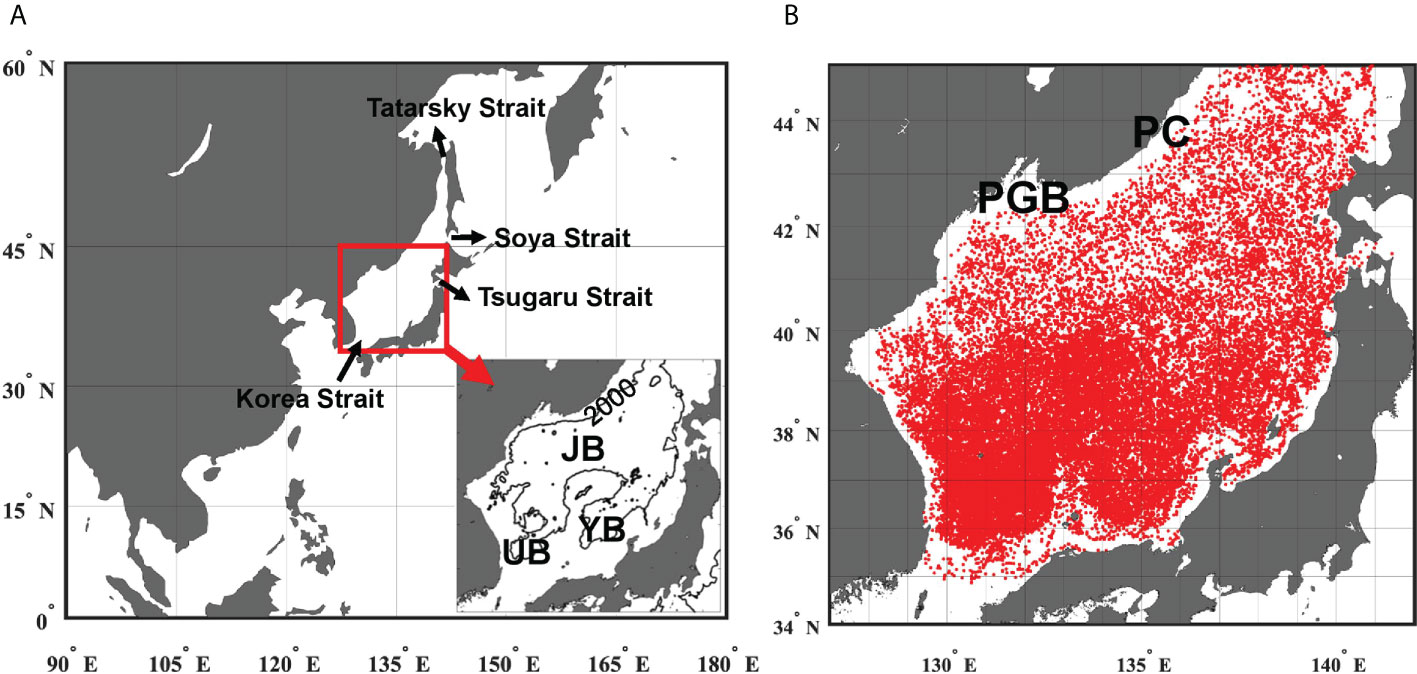
Figure 1 (A) Study region (red box) in the Northwestern Pacific. The black arrows indicate straits and their directions reflect schematic directions of surface current. The inset indicates the study region where the black contour denotes 2000 m isobath: JB, Japan Basin; YB, Yamato Basin; and UB, Ulleung Basin. (B) Station map shows locations of Argo float data from 2000 to 2020. The PGB and PC are abbreviations for the Peter the Great Bay and Primorye Coast, respectively.

As a deep marginal sea, the ES has its own meridional overturning circulation (MOC) composed of northward penetrations of the Tsushima Warm Water from the Korea Strait (above 200 m), and relatively colder and denser southward streams of water masses formed in the northern ES (below 200 m) Talley et al., 2003; Kim et al., 2004; Postlethwaite et al., 2005; Park and Lim, 2018). The timescale of the ES meridional overturning circulation (EMOC) has been considered as shorter than 100 yr (Kumamoto et al., 1998; Kim et al., 2001), and according to the long-term hydrographic data, the EMOC has changed dramatically over recent decades in comparison to that of the global oceans (Kim et al., 2001; Kang et al., 2003; Yoon et al., 2018). Thus, it is important to monitor changes in the EMOC for characterizing and predicting future changes in global MOCs in a warming world.

The southward streams of the EMOC mainly consist of the East Sea Intermediate Water (ESIW), East Sea Central Water (ESCW), and East Sea Bottom Water (ESBW; Kim et al., 2004; Postlethwaite et al., 2005; Park and Lim, 2018). The ESIW, a main component of the upper EMOC, is formed in the western JB, where negative wind stress curl (clockwise) is strongly developed over the winter period (Park and Lim, 2018). The negative wind stress curl induces Ekman downwelling, mainly driving the subduction of the ESIW from the surface to the intermediate layer (Kim and Kim, 1999; Park and Lim, 2018). The ESCW and ESBW are the main components of the lower EMOC and are mainly produced in the northern part of the central ES through open-ocean and shelf convections during the winter, respectively (Talley et al., 2003; Yoon et al., 2018). The winter ocean surface conditions, especially sea surface temperatures (SSTs) in the northern ES, are important parameters for identifying the responses of the EMOC to climate change.

As there are many global SST products, their local biases must be identified and corrected through comparisons with in-situ observational ocean data (i.e., ships, Argo floats, and ocean buoys). To reduce their biases, numerous efforts have been made using in-situ observational data for developing computation algorithms (Reynolds et al., 2002; Zhang et al., 2004; Reynolds et al., 2007; Huang et al., 2013; Huang et al., 2015; Huang et al., 2021). Such bias corrections have contributed to predicting large-scale air-sea interaction processes in the Pacific and Atlantic Oceans, such as El Niño-Southern Oscillation, and the Intertropical Convergence Zone (Siongco et al., 2020; Lee et al., 2022) however, biases of the reproduced SST products in the ES are poorly understood and few bias correction methods for SST in the ES have been suggested (Park et al., 2008; Park et al., 2015). Although it has been shown that the long-term trends of SST products in the ES are similar to those of ship-based data (R² = 0.67), this result was obtained in the UB (Lee and Park, 2019), where warm SSTs largely persist throughout the year.

Thus, in the present research, the focus is placed on evaluating the bias of SST products in the ES via comparison with Argo float data, especially for the long-term SST dataset, and deriving a bias correction method for this regional product. The remainder of the paper is organized as follows: In Section 2, the Argo float data and SST products are introduced; In Section 3, biases of optimally interpolated sea surface temperature (OISST) products in the ES are identified, a bias correction method using Argo float data is proposed, and the impact of the SST correction on winter conditions in the northern ES is also investigated; Section 4 summarizes the results and suggests future works.

Data

Argo float data

Argo float data were used as the reference for correcting biases of SST products in the ES (Figure 1B). Data quality of Argo temperature and pressure has been improved by following the delay-mode quality control, as suggested by the Argo data management teams (Wong et al., 2014), but the parameters employed for spike and inversion detection in Park and Kim (2007). Note that all floats with truncation issues for any negative surface pressure drift so called as Truncated Negative Pressure Drift issue were excluded from this analysis. The delayed mode quality control of temperature and pressure (provided surface pressure information was available) was conducted according to the Argo Data Management Team technical report (Park and Lim, 2018).

Argo temperature data from August 1999 to December 2020 were utilized. To directly compare Argo data with SSTs, temperatures at 5 m were estimated from Argo data (hereafter, ARSST) under the assumption that the mixed layer depth was deeper than 8 m. As the shallowest measurement from most Argo floats in the ES was approximately 4 m, the ARSST was estimated via linear interpolation if the top depth of the Argo profile data was shallower than 5 m. Argo profile data whose top depth was deeper than 8 m were excluded for this analysis. Notably, the primary findings of this research are insensitive to this mixed layer assumption, as the focus is on the bias of cold SST which appears mainly in winter (see Section 3). In the winter, strong northwesterly winds > 5 m/s (winter monsoon) normally blow from Russia to the ES, deepening the mixed layer depth in the ES. The wind-driven mixing greatly reduces the difference between bulk temperature and skin temperature.

Satellite SST products

To evaluate the biases of SST products in the ES, three SST products were used in the present study. First was the daily OISST (v.2), as provided by the National Oceanic and Atmospheric Administration (Reynolds et al., 2007; Huang et al., 2021). OISST data spans from September 1981 to December 2020 and has a 0.25° spatial resolution. The second was the daily optimally interpolated products of microwave-infrared SST (MWSST) provided by Remote Sensing Systems (Reynolds and Smith, 1994). MWSST has a data period from June 2002 to August 2017, and a 9 km spatial resolution. Third, the daily Operational SST and Sea Ice Analysis (OSTIA) provided by the United Kingdom Met Office (Stark et al., 2007) spans from April 2006 to December 2020 and has a 0.053° spatial resolution.

Among the three SST products, OISST covers the longest period, and is thus more suitable for identifying long-term variation of surface conditions in the ES; therefore, this product was mostly used to investigate SST biases in the ES and develop a bias correction method. Notably, to compare OISST with Argo data, the former was subsampled at the Argo float data locations, which were neither evenly distributed in space nor time, and whose number of data points was less than those of the SST products (see the winter averaged SST Figure below). All further quality control measures consisted of the removal of all extreme outliers beyond five standard deviations.

Surface drifter data

To identify whether the warm biases of cold SST come from the difference between skin and bulk temperature, surface temperature obtained from satellite-tracked drifters were used in this study. The surface temperatures are measured at the bottom of the surface buoy (approximately 0.2 m below the sea surface), which are used for correction of satellite SST products. The Surface drifter data in the global ocean are provided by Atlantic Oceanographic and Meteorological Laboratory, National Oceanic and Atmospheric Administration, USA as Global Drifter Program (https://www.aoml.noaa.gov/phod/gdp/). The drifter data in the ES were extracted from the global dataset, spanning from Jan. 1996 to Dec. 2006.

Results

Bias identification in OISST

OISSTs at Argo data points within the ES showed a significant correlation with ARSST across the entire temperature range from 2000–2020 (R² = 0.95), and scatterplots displayed this strong linear relationship (slope ≈ 1, intercept ≈ 0), with no discernable biases (Figure 2A); however, exploring cold temperature ranges< 10°C more closely, the OISSTs skewed warmer than the reference ARSSTs (Figure 2B). Furthermore, to investigate whether there is a period-dependent relation between the OISSTs and ARSSTs, when splitting the analysis period into two groups (2000–2010; 2011–2020), these patterns were replicated in both periods (Figures 2B, 3A, B). Frequency histograms of the differences between OISST and ARSST for the two periods also showed that OISST cold waters< 5°C maintained apparent warm biases (Figures 3C, D). Although the histogram shape narrows over the recent period, the mean deviations of OISST from ARSST over the two time periods were 0.95°C and 0.82°C, respectively, with no statistically significant difference between them at the 99% confidence level (Figures 3C, D).

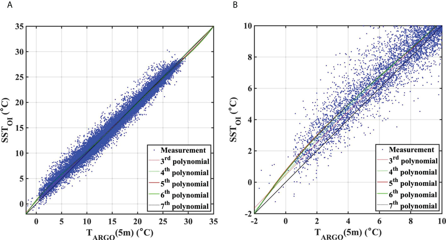
Figure 2 (A) Scatter plot of surface temperatures from Argo float data at 5 m (ARSST) and optimally interpolated sea surface temperature (OISST) at Argo data points. (B) Subplot of (A) for a temperature range of -2~10°C. Colored lines are n^th polynomial fits.

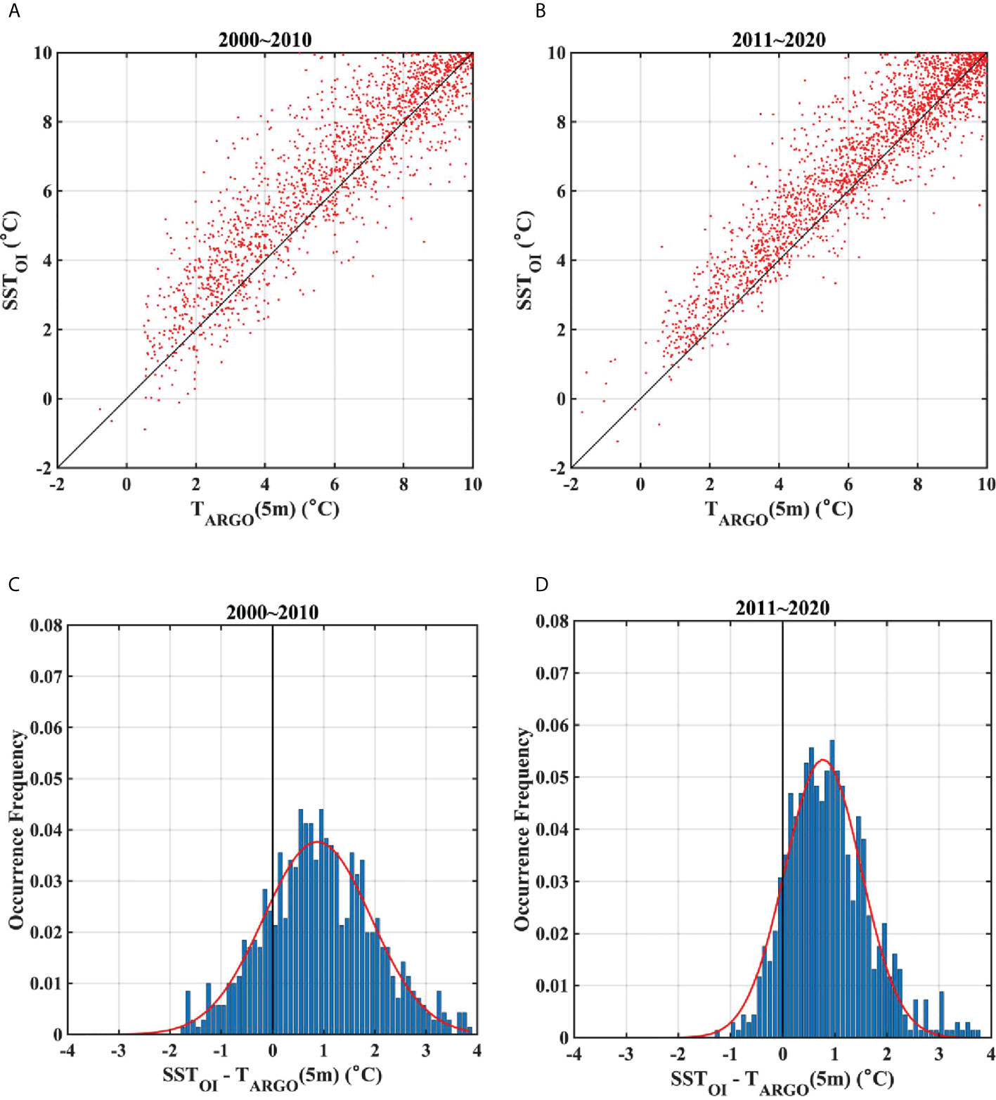
Figure 3 Surface temperatures from ARSST, and OISST at Argo data points ranging -2~10°C from (A) 2000–2010, (B) 2011–2020. (C, D) Frequency of differences between ARSST and OISST data for the temperature of less than 5°C in corresponding time ranges of (A, B), respectively. Red lines in (C) and (D) denote Gaussian functions fitted into each histogram.

When OISST was compared with ARSST obtained during day- and night-times, the warm bias of cold waters< 5°C was consistently identified in both cases (0.91°C and 0.95°C mean biases for day- and night-times, respectively; Figure 4). The features of histograms for the differences between OISST and ARSST during day- and night-times (Figures 4B, D) were very similar with those for the SST differences throughout the day (Figures 3C, D). In addition, the warm bias of the cold waters was also clearly shown at the differences between OISST and ARSST regardless of the periods in which strong or weak winds blow (1.03°C and 1.11°C mean biases for strong and weak wind cases, respectively; Figure 5). These results showed that the warm bias of the cold waters was not related to diurnal SST variations or wind strengths.

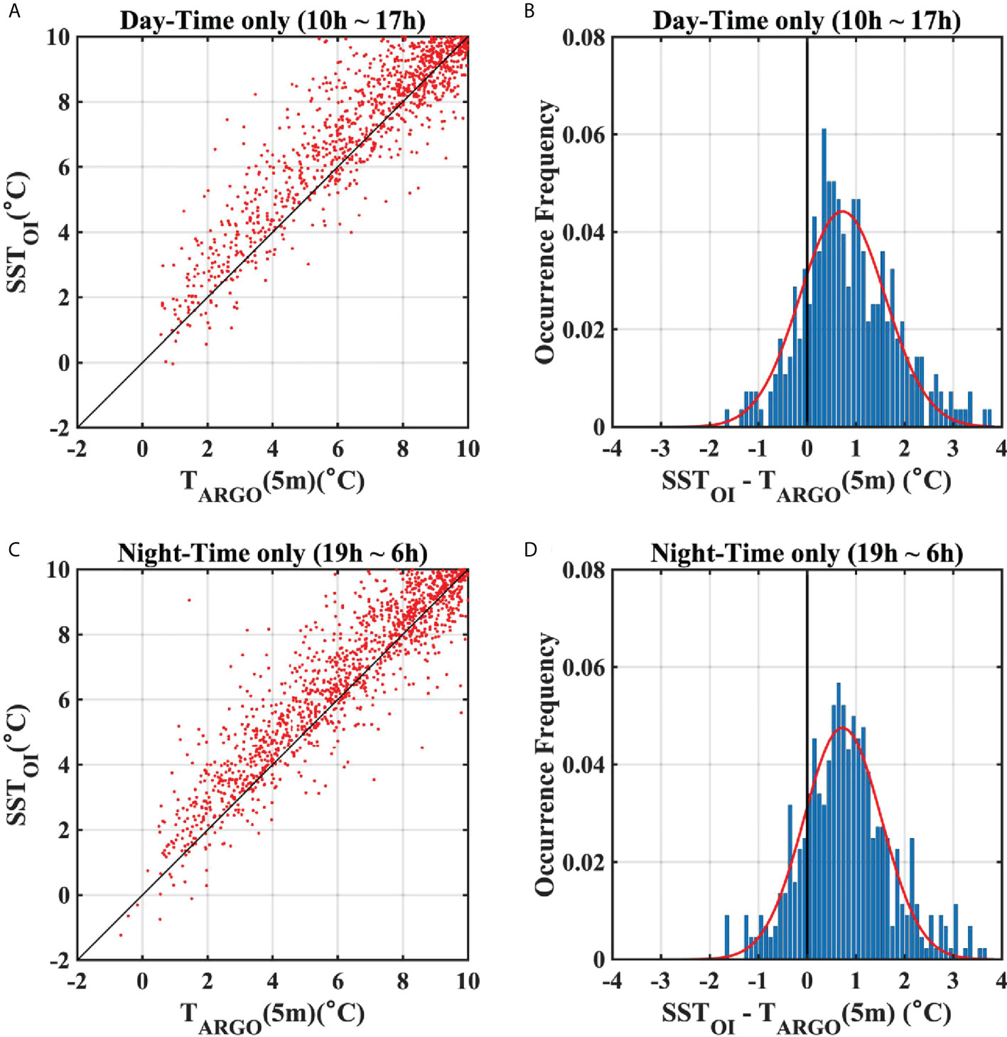
Figure 4 (A) Scatter plot of surface temperatures from ARSST, and OISST at Argo data points during day-time (10AM–5PM, local time). (B) Frequency of differences between ARSST and OISST data for a temperature range ofless than 5°C during day-time. (C) Same as (A), but for during night (7PM–6AM, local time). (D) Same as (B), but for during night-time.

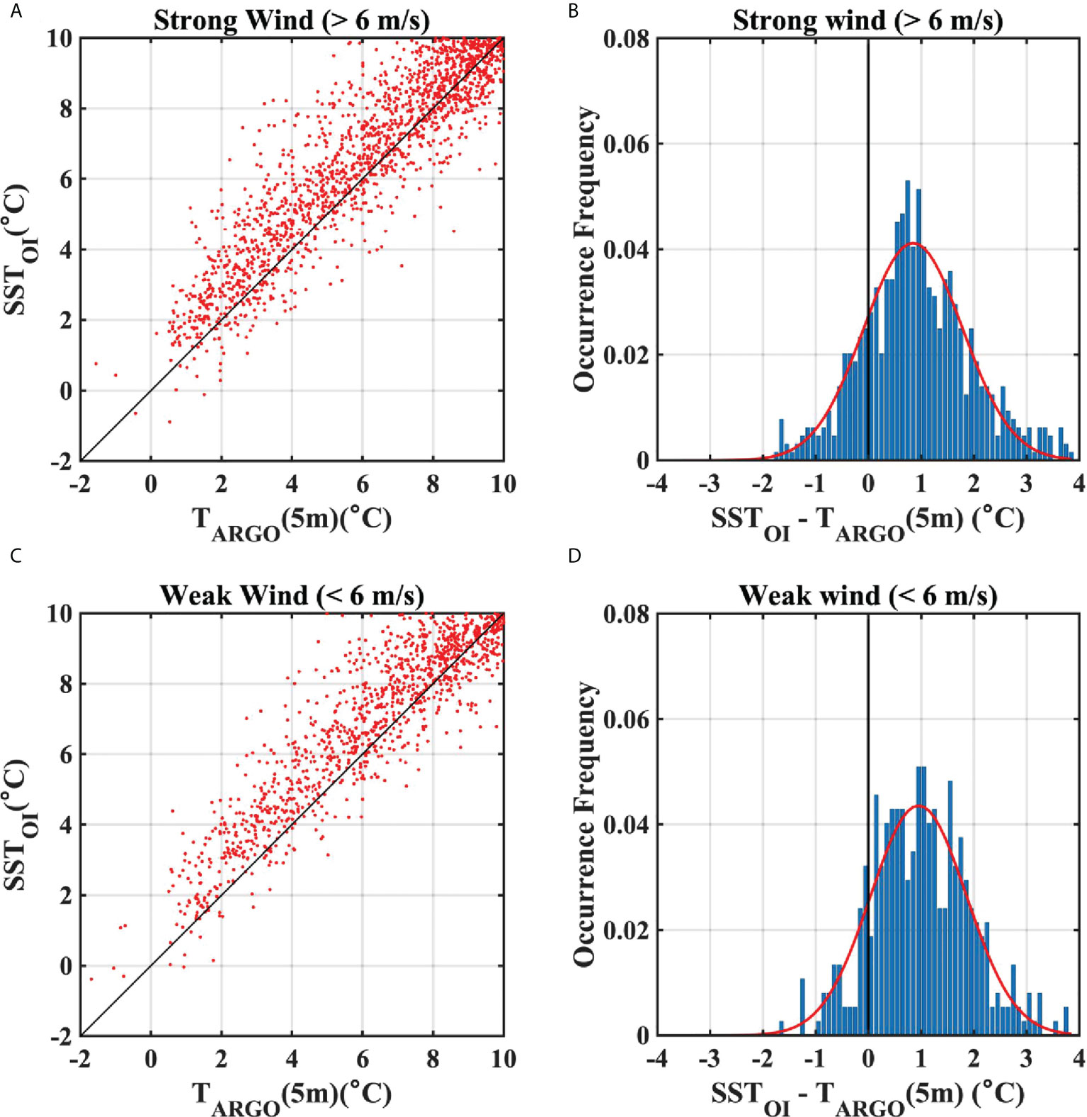
Figure 5 (A) Scatter plot of surface temperatures from ARSST, and OISST at Argo data points under strong wind (> 6m/s). (B) Frequency of differences between ARSST and OISST data for a temperature range of less than 5°C under strong wind. (C) Same as (A), but for under weak wind (< 6 m/s). (D) Same as (B), but for under weak wind.

The same analysis was also applied for OISSTs warmer than 15°C, although no similar significant biases were found (Figure 6), as all points were approximately linear over the two periods (Figures 6A, B). Further, the frequency of differences between OISSTs and ARSSTs from 15 to 20°C over the two time periods revealed no significant biases (Figures 6C, D). The mean deviation of OISSTs from ARSSTs for the two periods were near zero (-0.04°C and -0.14°C, respectively), and the slight cold biases observed during 2011–2020 were not statistically significant at the 99% confidence level (Figure 6D). Following these results, it was identified that OISST cold waters< 5°C had significant warm biases across the ES.

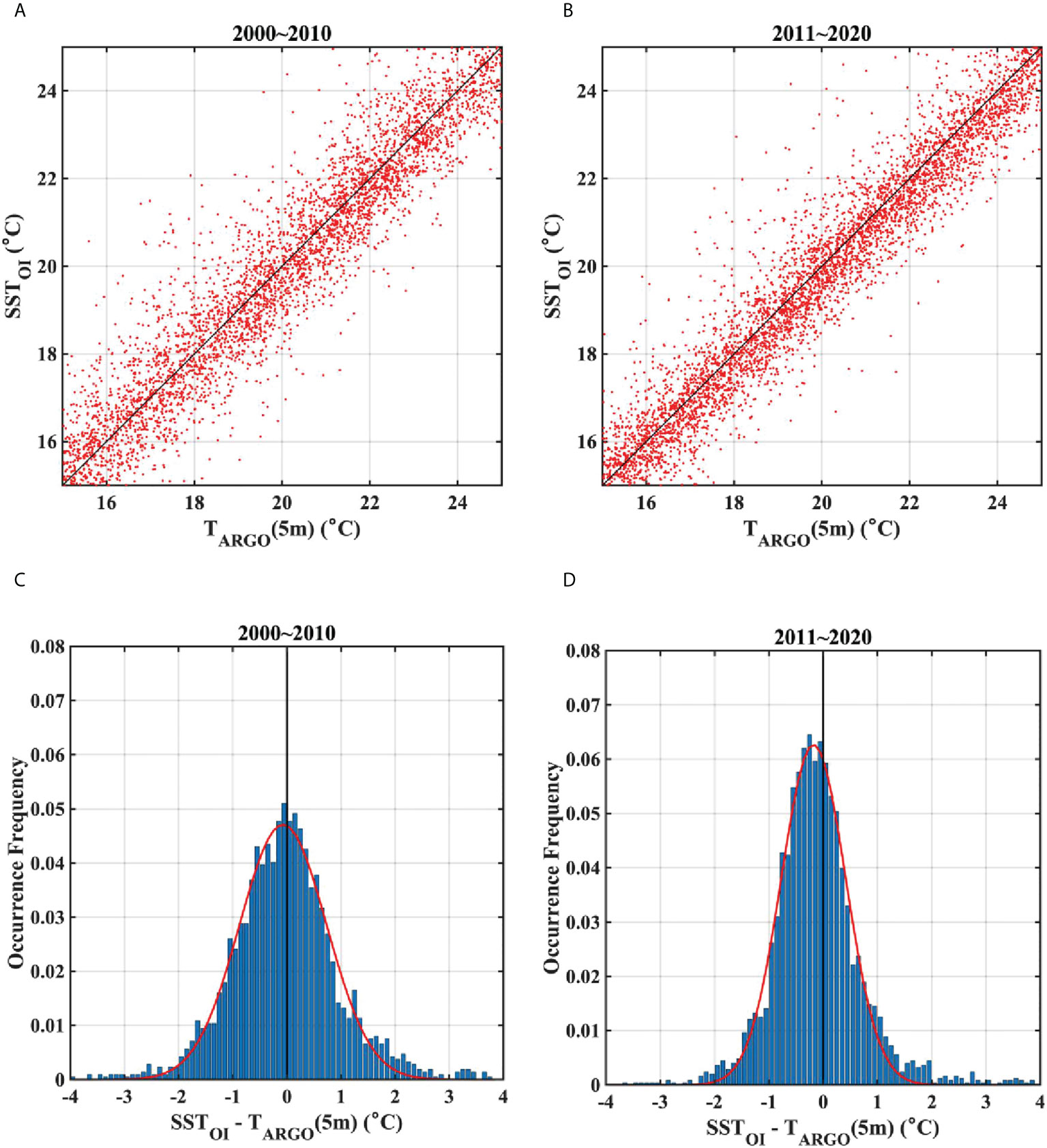
Figure 6 Surface temperatures from ARSST float data at 5 m, and OISST at Argo data points ranging 15~25°C from (A) 2000–2010, (B) 2011–2020. (C, D) Frequency of differences between ARSST and OISST data for the temperature of 15–20°C in corresponding time ranges of (A, B), respectively. Red lines in (C, D) denote Gaussian functions fitted to each histogram.

The comparison results between OISST and surface drifter data supported that the OISST cold waters had clear warm biases in the ES as well. The observational depth of surface drifter data is about 0.2, which is closer to the surface than that of ARSST (5 m), so surface drifter temperature could be considered as skin temperature at which the mixed layer depth issue can be ignored. Same as the results investigated above, OISST also had significant warm biases with surface drifter data, skin temperature, in the range of cold water< 5°C not in the whole temperature range (Figures 7A–D). The mean deviation of OISST from surface drifter data was 0.97°C similar with its mean deviation from ARSST.

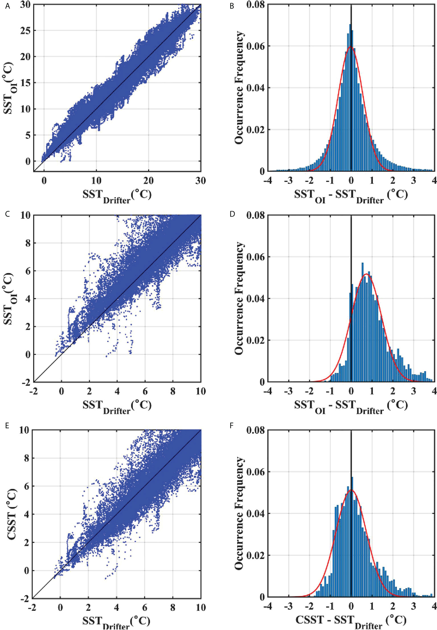
Figure 7 (A) Scatter plot of surface temperatures from surface drifters and OISST. (B) Frequency of differences between surface drifters and OISST data for the entire temperature range. (C) Subplot of (A) for a temperature range of -2~10°C. (D) Same as (B), but for a temperature range of less than 5°C. (E) Same as (C), but for corrected OISST. (F) Same as (D), but for corrected OISST.

Furthermore, such warm biases over colder temperature ranges were also observed for MWSSTs and OSTIA values (Figure 8). These products similarly displayed near-linear relationships with ARSSTs across the entire temperature range (Figures 8A, 8D); however, at ranges< 10°C or< 5°C, MWSST and OSTIA were slightly warmer than the reference (Figures 8B, C, E, F). Mean deviations of MWSST and OSTIA from ARSST were identical (0.36°C), notably less than that of OISST, although these biases of MWSST and OSTIA were significant at the 99% confidence level (Figures 8C, F).

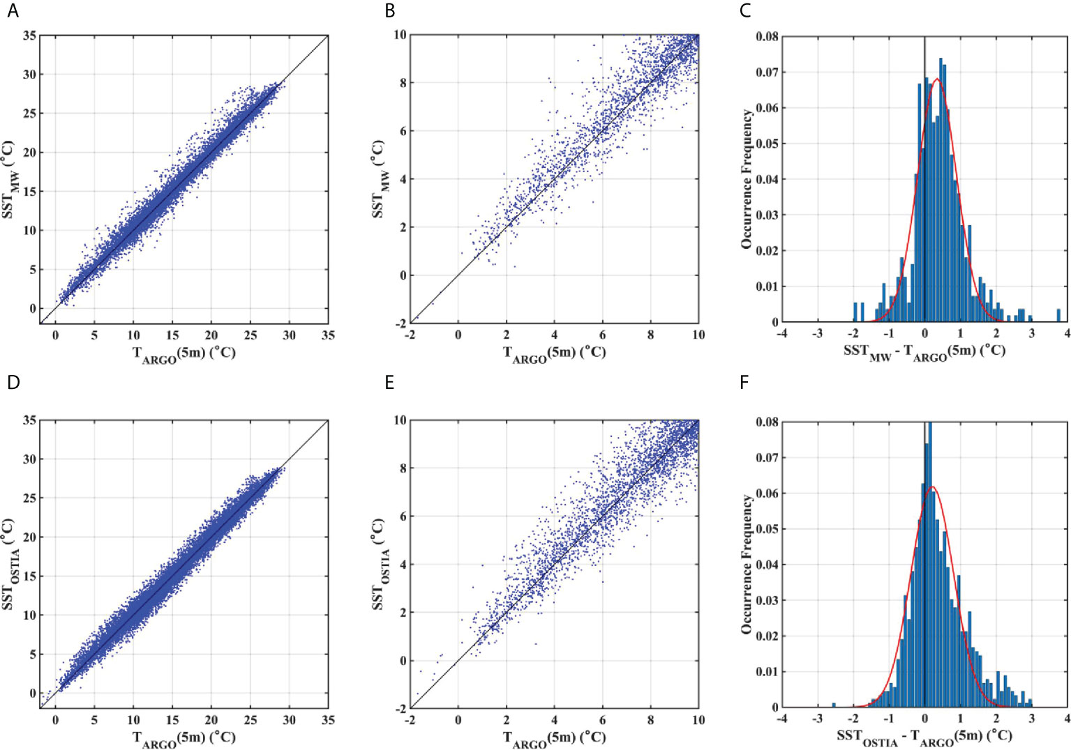
Figure 8 (A) Scatter plots of microwave-infrared SST (MWSST) vs ARSST, (B) Subplot of (A) for -2–10°C, and (C) Difference between MWSST and ARSST for less than 5°C. (D–F) same comparisons, but for daily operational SST and ice analysis (OSTIA) vs ARSST. Red lines in (C, F) depict Gaussian fits.

Examining the median deviations of OISST, MWSST, and OSTIA from ARSST (0.84, 0.36, and 0.24°C, respectively), OSTIA maintained the lowest warm biases among the three products; however, the estimated Gaussian function for the frequency histogram of OSTIA was highly skewed (skewness $\tilde{\mu }$_{3 =} 0.58) in comparison to other two products (OISST $\tilde{\mu }$₃ = 0.36, MWSST $\tilde{\mu }$₃ = 0.02); Figures 3C, D, 8C, F). When OSTIA was subsampled by 0.25° × 0.25°, median deviations (Supplementary Figure 1) was a little increased to 0.27°C, but the skewness of the Gaussian function was highly risen to 0.84, indicating that the OSTIA biases from ARSST would not be related to higher spatial resolution of the OSTIA product than that of MWSST and OISST products. Accordingly, OSTIA biases would be more difficult to correct compared to those of OISST and MWSST. As MWSST has a shorter data period than OISST, the latter product appeared best for investigating the long-term variation of SSTs in the ES. Moreover, compared to other SST products, OISST has been widely used to investigate ocean events (ex) marine heat wave (e.g. Miyama et al., 2021)) of the ES without any awareness of its bias, thus, OISST is necessary to be validated here.

Correcting SSTs using argo float data

The inverse n^th-order polynomial fit method was applied to correct the warm biases of OISST. In general, OISST and ARSST are used as a predictor and target variables, respectively, as ARSST is regarded as the true value. The target ARSST values can be reproduced using OISST with an n^th order polynomial fitting function (F_n ; Eq. (1)). The best-fitting function (F^best ; Eq. (2)) was thus determined by minimizing the differences from the target variable:

where X is the OISST value, Y is the ARSST value, and $\widehat{Y}$is the corrected OISST. In this case, however, the best-fitting function was obtained as a higher-order polynomial, meaning that the fitting accuracy could be poor, and greater computational demand would be required for obtaining the best-fitting function. Thus, to improve both the fitting accuracy and computing time, the corrected OISST (CSST) was estimated using ARSST as a predictor variable via an inverse function (inverse function = n^th order polynomial function (G_n ); Eq. (3)):

To derive the CSSTs, the n^th-order polynomial fits [$G_n^{best}$; Eq. (4)] were estimated using ARSST to minimize the differences from OISST (least-squared fitting; Figure 2; Table 1). The fit lines were only derived across the range of -2–25°C, under the assumption that ARSSTs > 25°C were near identical to OISSTs. The root mean square difference (RMSD) between the n^th order fitting lines and OISSTs showed strong similarities among functions, provided that a 3^rd order or higher was used over temperature ranges of 0–25°C and 0–5°C (Table 1, first and second columns).

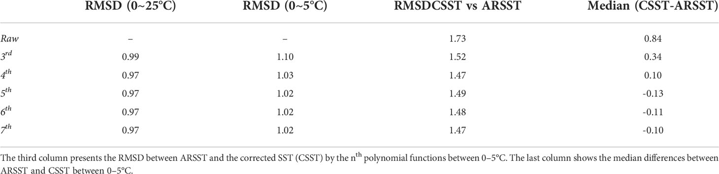
Table 1 Root mean square difference (RMSD) of n^th polynomial fits between 0–20°C and 0–5°C in the first and second columns respectively.

After calculating the n^th-order polynomial fits via Eq. (4), the best-fitting function (G^best ; Eq. (5)) which minimized the differences with ARSST was chosen among multiple solutions. The RMSD and median difference values between CSST and ARSST were the lowest when CSST was obtained by the 4^th-order polynomial function (Table 1). Moreover, frequency histograms of deviations between CSST and ARSST across the entire temperature range (-2–25°C) depicted that warm biases of OISST were best corrected by the 4^th-order polynomial function than other higher order polynomial functions (Figure 9). CSST also showed a significant decrease in mean and median deviations (0.24 and 0.09°C) from surface drifter data in the range of cold water< 5°C in comparison with the results between OISST and surface drifter data (Figures 7E, F). Accordingly, the warm biases of OISSTs were corrected using a 4^th-order polynomial function, thereby demonstrating that this method improved the fitting accuracy, and reduced CSST computational times when compared with the general polynomial fitting method.

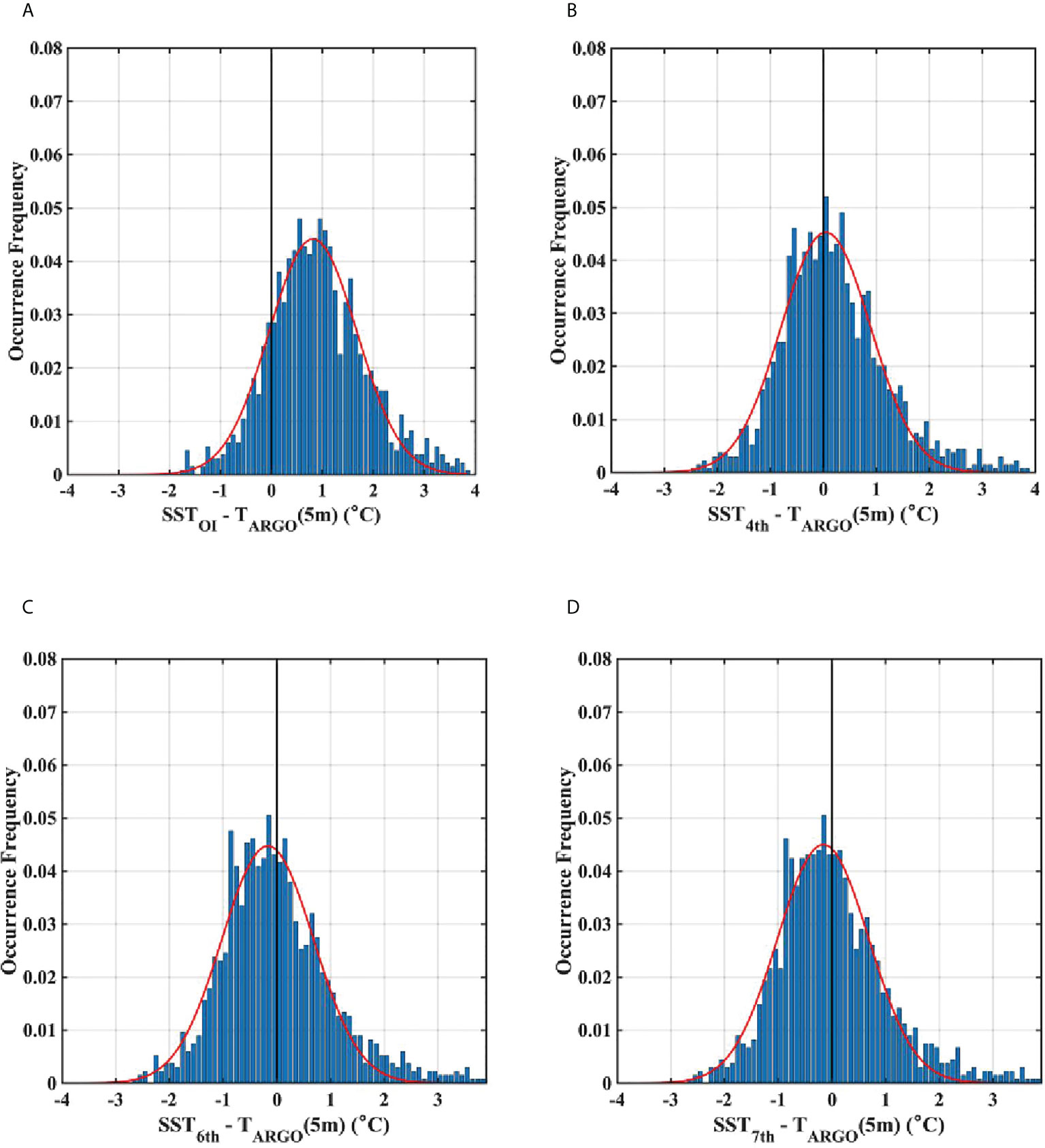
Figure 9 Differences between SST and ARSST for all temperature ranges (-2–25°C): (A) Original raw OISST data, (B) Corrected OISST (CSST) with the 4^th, (C) 6^th, and (D) 7^th polynomial functions. Red lines denote Gaussian fits.

Influence of SST correction on the ES

Averaged SST maps for the winter (Jan–Mar) of ARSSTs, OISSTs, and CSSTs were compared to identify the effects of correction on SST distributions in the ES (Figure 10; refer acronyms in Table 2). Although it was difficult to confirm the influence of correction across the entire domain of the ES due to large SST differences between the southern and northern ES, CSSTs showed colder temperatures in the northern ES than OISST, particularly towards the center of the JB and near the Primorye coast (Figures 10B, C), thereby aligning more closely with ARSSTs (Figure 10). As winter SST variations in the ES typically reach 15°C (Park and Lim, 2018), substantially larger than the warm bias in cold waters (Figures 3, 5), the impacts of SST corrections may only be observable in colder waters of the northern ES. Thus, this relatively minor difference between OISSTs and CSSTs over a basin-wide average (Figure 10) may explain why warm biases of cold SSTs were largely ignored by previous researchers.

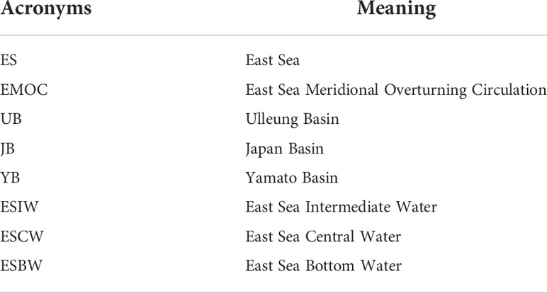
Table 2 Acronyms in the East Sea.

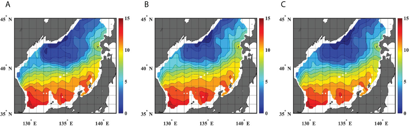
Figure 10 Surface temperatures from: (A) ARSST climatologically averaged for the winter (Jan.–Mar.) from 2000 to 2020, (B) OISST at Argo data points, and (C) CSST. Contour intervals are 1°C.

To further investigate the influence of SST corrections on the cold surface water, the frequency of winter outcropping areas was computed from the SST datasets for the ES (Figures 11–13). The outcropping areas represent regions for which temperatures of intermediate or deep layer water masses during the winter appear at the surface, and are often used as an indicator of formation rate of specific water mass (Petit et al., 2020). As discussed in Section 2, water masses that constitute the southward streams of the EMOC are formed at the surface of the northern ES. Specifically, the ESIW, the main component of the upper EMOC, is characterized by temperature ranges from 1 to 5°C (Kim et al., 2004; Park and Lim, 2018); whereas ESCW and ESBW, the primary components of the lower EMOC, maintain temperatures< 1°C (Kim et al., 2004; Yoon et al., 2018). Therefore, the occurrence frequency of outcropping areas was estimated based on these temperature criteria.

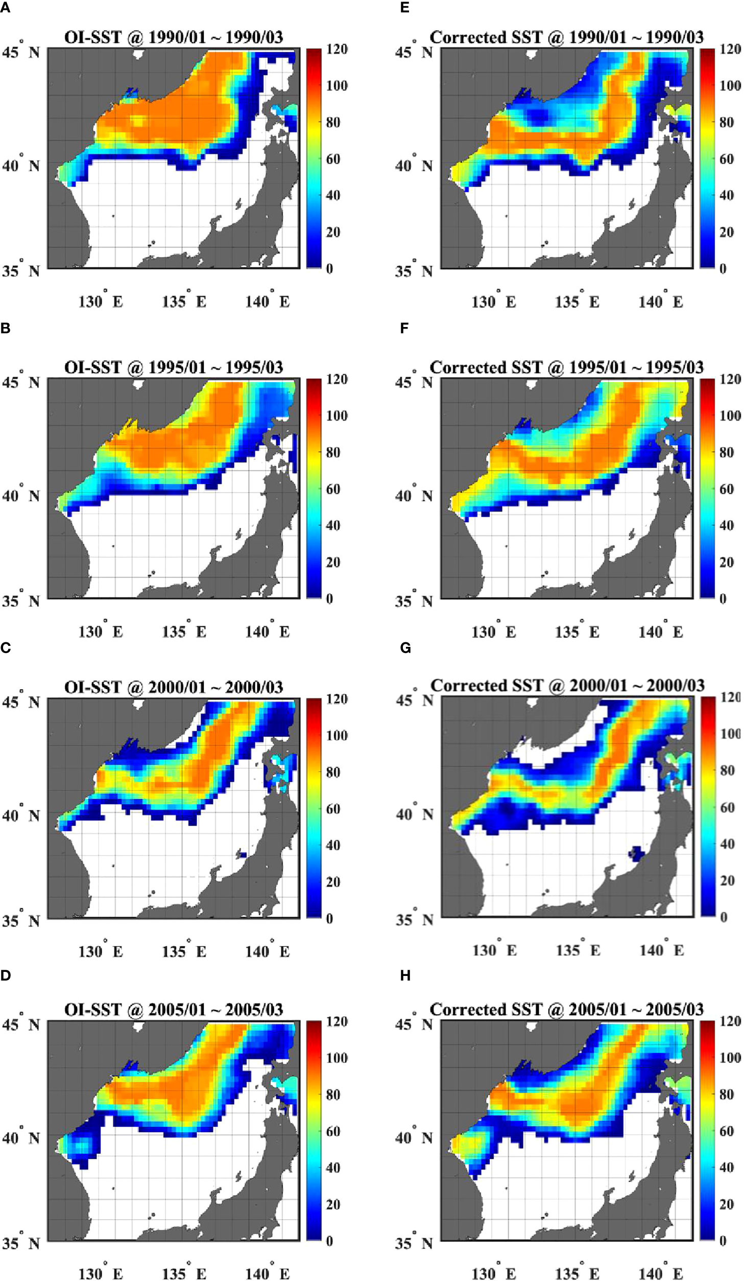
Figure 11 Day-counts when OISSTs were 1–5°C during the winter (Jan.–Mar.) in (A) 1990, (B) 1995, (C) 2000, and (D) 2005. (E–H) are same, but for CSST. Units are days.

Firstly, CSSTs consistently exhibited higher chances of outcropping for the ESIW during the winter at the western JB, widely considered the formation site of the ESIW (40.5°–42° N, 130°–132° E; Park and Lim, 2018), than the warm biased OISSTs, as shown in the maps of day-counts where each grid had 1–5°C during the winters of 1990, 1995, 2000, and 2005 (Figure 11). Furthermore, before the correction, OISSTs showed higher winter outcropping probabilities of the ESIW off the Peter the Great Bay, and along the Primorye coast (Figures 11A–D). These areas are widely regarded as the formation sites of the ESCW and ESBW (< 1°C) through deep convections, rather than the ESIW (Talley et al., 2003; Yoon et al., 2018). Conversely, CSSTs displayed remarkably lower outcropping likelihoods of the ESIW in these locations, indicating that the overestimate of outcropping probabilities of the ESIW in the northernmost ES was successfully adjusted through warm bias correction (Figures 11E–H).

The other SST products (MWSST and OSTIA) also showed similar distributions of total outcropping days for the ESIW with OISST, indicating that they underestimated the outcropping probabilities of the ESIW at the western JB, and overestimated its likelihood in the northernmost ES due to the warm biases of cold waters (Figures 5, 12). Notably, the MWSSTs did not produce signals near the Russian coast due to data availability (Figures 12B, F). Additionally, CSSTs detected relatively lower outcropping chances of the ESIW at the eastern JB (40.5°–42° N, 134°-136° E) than other SST products in the winter of 2015. As this region is considered the formation site of other intermediate water (e.g., High Salinity Intermediate Water) that is relatively colder (~ 0.6°C) and saltier (> 34.07) than the ESIW (1–5°C and < 34.06; Kim and Kim, 1999; Watanabe et al., 2001; Kim et al., 2004), this feature was also considered to be due to the warm bias correction.

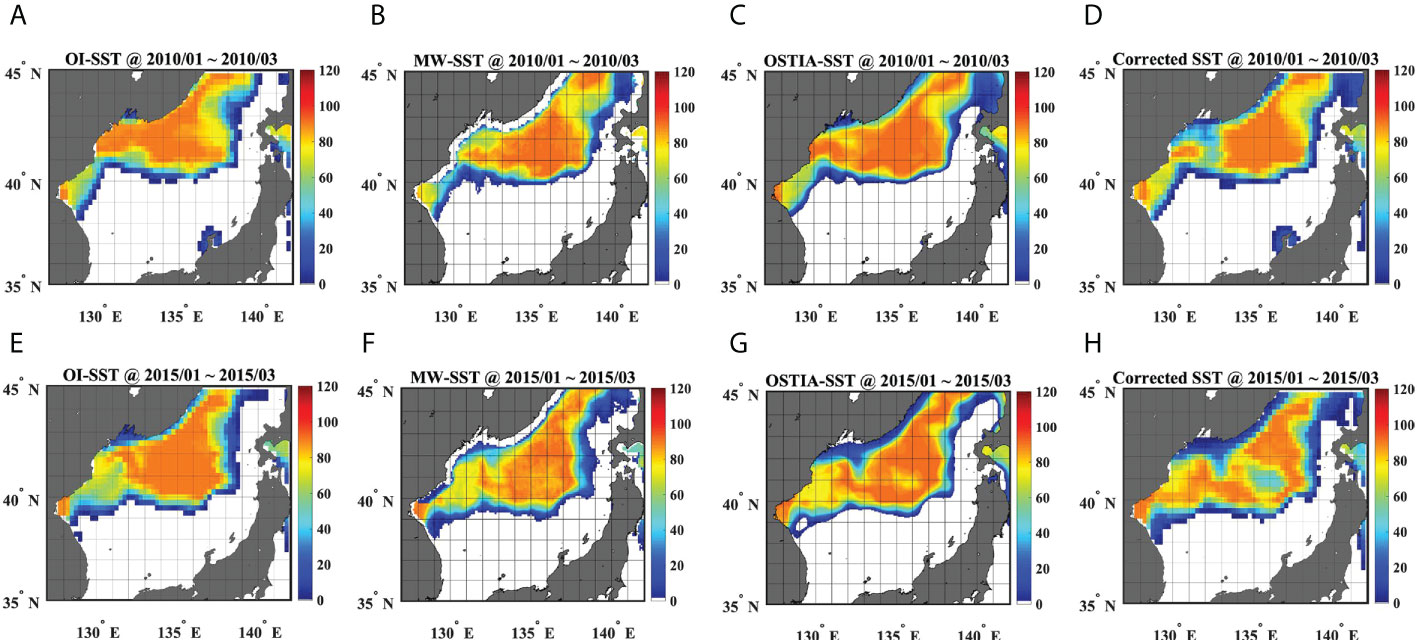
Figure 12 Day-counts when OISSTs were 1–5°C during the winter (Jan.–Mar.) in 2010 (upper row) and 2015 (lower row) for (A, E) OISST, (B, F) MWSST, (C, G) OSTIA, and (D, H) CSST. Units are days.

The annual characteristics of CSSTs and each SST product were also represented by the average day-counts of 1–5°C and<1°C outcroppings in the winters from 2007 to 2016 (Figure 13). CSSTs showed higher outcropping probabilities of the ESIW at the western JB, lower chances of the ESIW at the eastern JB, and significantly lower (higher) outcropping probabilities of the ESIW (ESCW and ESBW) off the Peter the Great Bay and along the Primorye coast than OISST, MWSST, and OSTIA (Figure 13). In conclusion, in-situ yearly and period-mean results of cold surface water occurrence revealed that CSSTs successfully captured the outcropping probabilities of ESIW, ESCW, and ESBW during the winter better than any of the three SST products at the correlated formation sites of those water masses (Kim et al., 2004; Park and Lim, 2018; Yoon et al., 2018), implying that the warm bias corrections can improve the capacity of SST products to identify the variations of the EMOC in a warming world.

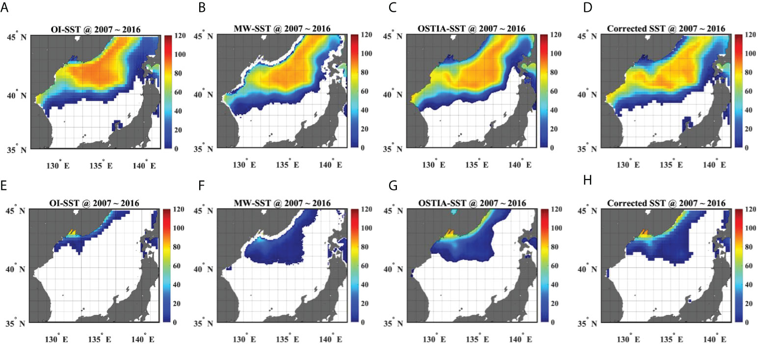
Figure 13 Average day-counts of 1–5°C outcropping in winter (Jan.–Mar.) from 2007–2016 for (A) OISST, (B) MWSST, (C) OSTIA, and (D) CSST. Average day-counts of less than 1°C outcropping for (E) OISST, (F) MWSST, (G) OSTIA, and (H) CSST. Units are days.

Discussion & Conclusion

This study identified warm biases from three global SST products (OISST, MWSST, and OSTIA) only for the cold surface waters of the ES. Among them, the long-term OISSTs were corrected using Argo float temperature data via a novel, simplistic, and effective inverse polynomial fitting method. The resulting corrected SST datasets were accurately depicted the regional variation in the northern ES compared to non-corrected products; thus, these results emphasized the importance of regional corrections for global SST products via in-situ observational data.

The reason why warm bias of only cold SST occurred is unclear. In general, skin temperatures obtained from satellite measurements are higher than bulk temperatures like what Argo floats measure, especially when positive heat flux (heat transferring from atmosphere to ocean) is dominant under calm weather. However, in the ES, the cold SST (below 5°C) only appears in wintertime when negative flux prevails. Indeed, there are neither significant differences of warm bias in cold SST between day-time and night-time (Figure 4) nor between weak wind and strong wind conditions (Figure 5). Furthermore, even comparing with temperatures measured by surface drifter, there is a clear warm bias of cold SST in the OISST comparable to the comparison result with Argo float (Figures 3, 7). In near future, it is needed to investigate the reason for occurrence of warm biases in the ES from SST products during winter.

Biases from SST products not only create difficulty when analyzing observational data, but have important implications for the production of climate reanalysis products on heat and fresh-water fluxes utilizing the satellite SST data as well. Furthermore, numerous ocean circulation models employ flux data from these reanalysis products for boundary forcing. As identified in Section 3.3, any numerical model forced with non-corrected SST products may represent higher formation rates of water masses in the upper EMOC (i.e., ESIW), and lower formation rates in the lower EMOC (i.e., ESCW and ESBW). Similarly, when uncorrected SST data are assimilated into the ocean prediction model, such SST biases could produce unrealistic EMOC patterns; thus, it is necessary to reproduce the ES reanalysis products using CSSTs in the future to improve regional ocean model predictive performance regarding the variation of the EMOC under a warming world.

Additionally, as shown by the median value comparisons of frequency (Figures 3, 6), OSTIA SSTs were more comparable to ARSSTs than OISSTs or MWSSTs. Similarly, the spatial distribution of outcropping days in Figure 13 obtained from OSTIA was relatively similar to that of CSST; thus, among non-corrected SST products, OSTIA most accurately depicted the surface conditions of the northern ES in the winter. Unfortunately, the biases of OSTIA cannot be corrected solely with the suggested polynomial fitting method due to the high observed skewness of bias distributions (as shown in the frequency of differences from ARSST; Figures 8D–F). OSTIA SSTs have been produced by merging various satellite SSTs, as well as available in-situ measurements; thus, employing CSSTs in the production of OSTIA SSTs could significantly improve its accuracy in the ES.

Many other SST products have been newly produced and updated apart from three SST products discussed here, especially the long-term (from 1981 to the present) SST product from European Space Agency Climate Change Initiative (ESA CCI) is one of them (Merchant et al., 2019; Yang et al., 2021). ESA CCI SST product has not been used in the research of the ES yet, however, it was found that this product had no warm bias with ARSST in the range of cold water< 5°C and the Gaussian function of histogram for the difference between ESA CCI SST and ARSST had relatively lower skewness (Supplementary Figure 2). ESA CCI SST is considered to have a great potential to investigate the ES, henceforward, it would greatly help to investigate the long-term variation of the EMOC.

It is unclear why SST products tend towards warm biases in the colder temperature ranges, and whether this bias is apparent in other high latitudes or marginal seas as well. Due to the limited availability of in-situ datasets, the spatio-temporal characteristics of these SST biases were not investigated any further here, although the OISST did display a consistent bias over time (both before and after 2010). In the future, sub-regional correction algorithms should be developed for adjusting any spatio-temporally dependent biases of SST products in the ES and other seas via the inclusion of additional in-situ observational data and improved statistical methods.

Data availability statement

Publicly available datasets were analyzed in this study. This data can be found here: NOAA High-Resolution SST data was provided by the NOAA/OAR/ESRL PSL, Boulder, Colorado, USA (https://psl.noaa.gov/). Microwave OI SST data were produced by Remote Sensing Systems and sponsored by the National Oceanographic Partnership Program (NOPP) and the NASA Earth Science Physical Oceanography Program (www.remss.com). UK Met Office. 2005. OSTIA L4 SST Analysis. Ver. 1.0. PO. DAAC, CA, USA. (see webpage for the appropriate citation, https://podaac.jpl.nasa.gov/CitingPODAAC). The Argo data were collected and made freely available by the International Argo Program and the National programs that contribute to it (http://www.argo.ucsd.edu, http://argo.jcommops.org).

Author contributions

JP: conceptualization, data acquisition, formal analysis, visualization, project administration; S-TY: writing original draft; JP and S-TY: investigation, writing-review, and editing. All authors contributed to the article and approved the submitted version.

Funding

This research was a part of the project titled “Development of the core technology and establishment of the operation center for underwater gliders” funded by the Ministry of Oceans and Fisheries, Korea (1525012198). S-TY was supported by the NRF grant funded by the Ministry of Education (2022R1I1A3063629).

Conflict of interest

The authors declare that the research was conducted in the absence of any commercial or financial relationships that could be construed as a potential conflict of interest.

Publisher’s note

All claims expressed in this article are solely those of the authors and do not necessarily represent those of their affiliated organizations, or those of the publisher, the editors and the reviewers. Any product that may be evaluated in this article, or claim that may be made by its manufacturer, is not guaranteed or endorsed by the publisher.

Supplementary material

The Supplementary Material for this article can be found online at: https://www.frontiersin.org/articles/10.3389/fmars.2022.965346/full#supplementary-material

References

Gamo T. (2011). Dissolved oxygen in the bottom water of the Sea of Japan as a sensitive alarm for global climate change. Trends Anal. Chem. 30, 1308–1319. doi: 10.1016/j.trac.2011.06.005
Gamo T., Nakayama N., Takahata N., Sano Y., Zhang J., Yamazaki E., et al. (2014). The Sea of Japan and its unique chemistry revealed by time-series observations over the last 30 years. Monogr. Environ. Earth Planets 2, 1–22. doi: 10.5047/meep.2014.00201.0001
Han S., Hirose N., Usui N., Miyazawa Y. (2016). Multi-model ensemble estimation of volume transport through the straits of the East/Japan Sea. Ocean Dyn. 66, 59–76. doi: 10.1007/s10236-015-0896-9
Huang B., L’Heureux M., Lawrimore J., Liu C., Zhang H.-M., Banzon V., et al. (2013). Why did large difference arise in the sea surface temperature datasets across the tropical pacific during 2012? J. Atmos. Ocean. Technol. 30, 2944–2953. doi: 10.1175/JTECH-D-13-00034.1
Huang B., Liu C., Banzon V., Freeman E., Graham G., Hankins B., et al. (2021). Improvements of the daily optimum interpolation sea surface temperature (DOISST) version 2.1. J. Clim. 34, 2923–2939. doi: 10.1175/JCLI-D-20-0166.1
Huang B., Wang W., Liu C., Banzon V., Zhang H.-M., Lawrimore J. (2015). Bias adjustment of AVHRR SST and its impact on two SST analyses. J. Atmos. Ocean. Technol. 32, 372–387. doi: 10.1175/JTECH-D-14-00121.1
Kang D.-J., Park S., Kim Y. G., Kim K., Kim K. R. (2003). A moving-boundary box model (MBBM) for oceans in change: An application to the East/Japan Sea. Geophys. Res. Lett. 30, 32–1–32-4.doi: 10.1029/2002GL016486
Kim Y. G., Kim K. (1999). Intermediate waters in the East/Japan Sea. J. Oceanogr. 55, 123–132.doi: 10.1023/A:1007877610531
Kim K., Kim K. R., Kim Y. G., Cho Y. K., Kang D. J., Takematsu M., et al. (2004). Water masses and decadal variability in the East Sea (Sea of Japan). Prog. Oceanogr. 61, 157–174. doi: 10.1016/j.pocean.2004.06.003
Kim K., Kim K. R., Min D. H., Volkov Y., Yoon J. H., Takematsu M. (2001). Warming and structural changes in the East (Japan) Sea: A clue to future changes in global oceans? Geophys. Res. Lett. 28 (17), 3293–3296.doi: 10.1029/2001GL013078
Kumamoto Y. I., Yoneda M., Shibata Y., Kume H., Tanaka A., Uehiro T., et al. (1998). Direct observation of the rapid turnover of the Japan Sea bottom water by means of AMS radiocarbon measurement. Geophys. Res. Lett. 25, 651–654.doi: 10.1029/98GL00359
Lee J., Kang S. M., Kim H., Xiang B. (2022). Disentangling the effect of regional SST bias on the double-ITCZ problem. Clim. Dyn. 58, 3441–3453. doi: 10.1007/s00382-021-06107-x
Lee E. Y., Park K. A. (2019). Change in the recent warming trend of sea surface temperature in the East Sea (Sea of Japan) over decades, (1982–2018). Remote Sens. 11,2613, 1–17. doi: 10.3390/rs11222613
Merchant C. J., Embury O., Bulgin C. E., Block T., Corlett G. K., Fiedler E., et al. (2019). Satellite-based time-series of sea-surface temperature since 1981 for climate applications. Sci. Data 6, 223. doi: 10.1038/s41597-019-0236-x
Miyama T., Minobe S., Goto H. (2021). Marine heatwave of sea surface temperature of oyashio region in summer in 2010-2016. Front. Mar. Sci 7, 576240. doi: 10.3389/fmars.2020.576240
Park J. J., Kim K. (2007). Evaluation of calibrated salinity from profiling floats with high resolution conductivity-temperature-depth data in the East/Japan Sea. J. Geophys. Res. Oceans 112, C05049. doi: 10.1029/2006JC003869
Park K.-A., Lee E.-Y., Li X., Chung S.-R., Sohn E.-H., Hong S. (2015). NOAA/AVHRR sea surface temperature accuracy in the East/Japan Sea. Int. J. Digit. Earth 8 (10), 784–804. doi: 10.1080/17538947.2014.937363
Park J. J., Lim B. (2018). A new perspective on origin of the East Sea intermediate water: Observations of argo floats. Prog. Oceanogr. 160, 213–224. doi: 10.1016/j.pocean.2017.10.0151667
Park K.-A., Sakaida F., Kawamura H. (2008). Oceanic skin-bulk temperature difference through the comparison of satellite-observed sea surface temperature and in-situ measurements. Kor. J. Remote Sens. 24 (4), 1–15. doi: 10.7780/kjrs.2008.24.4.2731668
Petit T., Lozier M. S., Josey S. A., Cunningham S. A. (2020). Atlantic Deep water formation occurs primarily in the Iceland basin and irminger sea by local buoyancy forcing. Geophys. Res. Lett. 47, e2020GL091028. doi: 10.1029/2020GL0910281669
Postlethwaite C. F., Rohling E. J., Jenkins W. J., Walker C. F. (2005). A tracer study of ventilation in the Japan/East Sea. Deep Sea Res. Part II Top. Stud. Oceanogr. 52 (11–13), 1684–1704. doi: 10.1016/j.dsr2.2004.07.0321670
Reynolds R. W., Rayner N. A., Smith T. M., Stokes D. C., Wang. W. (2002). An improved in situ and satellite SST analysis for climate. J. Climate 15, 1609–1625. doi: 10.1175/1520-0442(2002)015<1609:AIISAS>2.0.CO;2
Reynolds R. W., Smith T. M. (1994). Improved global sea surface temperature analyses using optimum interpolation. J. Climate 7, 929–948. doi: 10.1175/1520-0442(1994)007<0929:IGSSTA>2.0.CO;2
Reynolds R. W., Smith T. M., Liu C., Chelton D. B., Casey K. S., Schlax M. G. (2007). Daily high-resolution-blended analyses for sea surface temperature. J. Climate 20, 5473–5496. doi: 10.1175/2007JCLI1824.1
Siongco A. C., Ma H. Y., Klein S. A., Xie S., Karspeck A. R., Raeder K., et al. (2020). A hindcast approach to diagnosing the equatorial pacific cold tongue SST bias in CESM1. J. Climate 33, 1437–1453. doi: 10.1175/JCLI-D-19-0513.1
Stark J. D., Donlon C. J., Martin M. J., McCulloch M. E. (2007). “OSTIA : An operational, high resolution, real time, global sea surface temperature analysis system,” in OCEANS 2007 - Europe, 2007. doi: 10.1109/OCEANSE.2007.4302251
Talley L. D., Lobanov V., Ponomarev V., Salyuk A., Tishchenko P., Zhabin I., et al. (2003). Deep convection and brine rejection in the Japan Sea. Geophys. Res. Lett. 30, 1159. doi: 1029/2002GL016451
Watanabe T., Hiari M., Yamada H. (2001). High-salinity intermediate water of the Japan Sea in the eastern Japan basin. J. Geophys. Res. 106 (C6), 11,437–11,450. doi: 10.1029/2000JC000398
Wong A., Keeley R., Carval T. (2014). Argo quality control manual (Argo Data Management). (Brest, France: IFREMER). doi: 10.13155/33951
Yang C., Leonelli F. E., Marullo S., Artale V., Beggs H., Nardelli B. B., et al. (2021). Sea Surface temperature intercomparison in the framework of the Copernicus climate change service (C3S). J. Clim. 34 (13), 5257–5283. doi: 10.1175/JCLI-D-20-0793.1
Yoon S. T., Chang K. I., Nam. S., Rho T., Kang D. J., Lee T., et al. (2018). Re-initiation of bottom water formation in the East Sea (Japan Sea) in a warming world. Sci. Rep. 8, 1576. doi: 10.1038/s41598-018-19952-4
Keywords: sea surface temperature, argo float data, satellite data, east sea, bias correction, outcropping
Citation: Yoon S-T and Park J (2022) Warm bias of cold sea surface temperatures in the East Sea (Japan Sea). Front. Mar. Sci. 9:965346. doi: 10.3389/fmars.2022.965346
Received: 09 June 2022; Accepted: 29 July 2022;
Published: 17 August 2022.
Edited by:
Kyung-Ae Park, Seoul National University, South KoreaReviewed by:
Christopher John Merchant, University of Reading, Reading, United KingdomBoyin Huang, National Centers for Environmental Information (NOAA), United States
Copyright © 2022 Yoon and Park. This is an open-access article distributed under the terms of the Creative Commons Attribution License (CC BY). The use, distribution or reproduction in other forums is permitted, provided the original author(s) and the copyright owner(s) are credited and that the original publication in this journal is cited, in accordance with accepted academic practice. No use, distribution or reproduction is permitted which does not comply with these terms.
*Correspondence: JongJin Park, jjpark@knu.ac.kr