Attribution of Plastic Sources Using Bayesian Inference: Application to River-Sourced Floating Plastic in the South Atlantic Ocean

Introduction

Floating plastic items have been found in all of the world’s oceans (Eriksen et al., 2014; Van Sebille et al., 2015), but the origins (i.e. where and when the plastic entered the ocean) of these plastic items are often not obvious. For some of the larger macroplastics, the origin can be attributed by careful analysis of labels [e.g. Lebreton et al. (2018); Schofield et al. (2020); Turner et al. (2021)], but most (micro)plastic particles are too small and nondescript for their origin to be identified this way. Nevertheless, it is important to assess and possibly attribute the likely source for these smaller particles too, as they represent a threat for marine ecosystems (Koelmans et al., 2019).

Here, we use numerical simulations to compute the pathways of virtual plastic particles that float on the surface of the ocean (Hardesty et al., 2017; van Sebille et al., 2018). By tracking particles, it is in principle possible to connect any source with any location. However, the multitude of possible sources very quickly makes this a computationally unwieldy approach. To overcome this computational challenge, here we propose using a Bayesian inference approach to attribute sources in a probabilistic sense.

Such a probabilistic approach has been used before to locate objects lost at sea, like the submarine Scorpio (Richardson et al., 1971) and the (yet to be found) Malaysian Airlines flight MH370 (Davey et al., 2016). The main difference between these search & rescue applications of Bayesian inference and our application in the source attribution of floating plastic is that the sources of plastic are spatially very heterogeneous, and so is their distribution at sea. With regards to plastic source attribution, van Duinen et al. (2021) took a similar approach in which they implemented a Bayesian framework to estimate the most likely sources that contribute to the plastic litter found on a beach in the North Sea. They performed a backtracking Lagrangian simulation from the beach towards the possible sources and combined this with estimates of plastic emitted at river mouths, fishing grounds, and coastlines. The main limitation with their implementation is that it focuses on one location rather than a whole domain.

As an illustration of this probabilistic framework for attribution of likely plastic sources, we apply it to plastic emitted by rivers around the South Atlantic Ocean, as rivers are considered the principal pathway for mismanaged plastic waste (MPW) into the ocean (Lebreton and Andrady, 2019). For clarity, we don’t consider other plastic sources such as plastic from fisheries or plastic from land (Jambeck et al., 2015). We selected the South Atlantic Ocean as the study location because the South Atlantic Subtropical Gyre is an accumulation zone for plastic (Morris, 1980; Cózar et al., 2014; Ryan, 2014), but also because of the presence of large urban centers along the American and African coast that contribute to the plastic found at sea (do Sul and Costa, 2007; Jambeck et al., 2018), and because this region was sampled during a 2019 expedition (Weckhuysen et al., 2021).

Data and Methods

Method

Bayesian inference uses Bayes’ Theorem to estimate the conditional probability of an event happening under certain conditions by combining prior knowledge about the problem with data obtained through an experiment. In particular, our objective is to estimate the probability that a particle sampled at sea would come from a certain source. This can be written as the conditional probability p(R_i|S_loc) : the probability of sampling a particle at a location S_loc from a specific source R_i . Bayes’ theorem offers a way of estimating p(R_i|S_loc) , by combining prior knowledge with new observations. In our case, Bayes’ theorem is

where p(R_i|S_loc) is the conditional probability that we aim to estimate, p(S_loc|R_i) is the opposite conditional probability that can be estimated by performing a numerical simulation (see below), p(R_i) is the probability of a particle being released at the R_i source and p(S_loc) is the probability of sampling a plastic particle at a specific location, regardless of the source. It is important to note that p(R_i|S_loc)≠p(S_loc|R_i). The latter term namely indicates the probability of a plastic particle found at a location to come from the source R_i , and the former indicates the probability of a particle coming from the source R_i being at a location. Each term is commonly referred to by its interpretation. For instance, p(R_i) is denoted as ‘the prior’ because it represents the prior knowledge of the problem, p(S_loc|R_i) is ‘the likelihood’, which updates our prior knowledge from the problem, p(S_loc) is the ‘normalizing constant’, and p(R_i|S_loc) is ‘the posterior’.

In eq. (1), computing the normalizing constant p(S_loc) requires observations for all plastics in the ocean regardless of their source, which means that p(S_loc) also considers plastic that comes from sources that are not taken into account in the numerator of eq. (1). Therefore, the posterior probabilities at each S_loc would not add to one in each location but instead will add to a fraction that corresponds only to the sources of plastic considered in the study. For the present study, this is inconvenient because our analysis is limited to plastic emitted by rivers and it does not consider plastic from other sources. To overcome this inconvenience, we can constrain the sum of all posterior probabilities to be equal to one

where the sum is defined for the N number of sources. Then, substituting p(R_i|S_loc) for eq. (1)

and by factorizing and solving for p(S_loc)

we obtain a normalizing constant that only considers the sum of all our hypotheses (i.e. products of prior and likelihoods). Finally, by substituting p(S_loc) in eq. (1) we get

which is an alternative form of Bayes’ theorem (Carlin and Louis, 2008) that ensures that the sum of all posterior probabilities is one in each location. This last equation is used in this study.

Prior Data and Selecting the Sources

Our prior is based on the annual amount of riverine plastic estimated by Meijer et al. (2021), who used a probability framework combined with geographical data of MPW to estimate the plastic mass emissions of the world rivers into the ocean, at the location of the river mouths. From their global data set, we selected the locations and annual emissions for all 1,010 rivers that emit plastic into the South Atlantic. To avoid immediate beaching, we moved the river mouth locations to the center of the closest ocean grid-cell of the model’s flow field, and when various rivers shared the same closest grid-cell, we summed their emissions. This condensed the number of river mouths to 535 (without affecting the total amount of plastic released by the rivers in the South Atlantic).

We then clustered the rivers in 10 groups that contained the top polluting rivers and their neighboring rivers. These clusters are 2° by 2° square regions centered around ten locations that coincide with important cities or river estuaries. They contain the river mouth locations of the rivers within their limits and we used these locations as release locations. The 10 clusters (Figure 1) account for 80.9% of the riverine plastic emissions in the South Atlantic. There are two clusters on the African coast: around the city of Cape Town and on the Congo River estuary. The other eight clusters are on the South American coast: five near the cities of Rio de Janeiro, Porto Alegre, Santos, Salvador, and Recife; and three on the river estuaries of Rio de la Plata, Itajaí and Paraibá. We also considered the 19.1% remaining rivers excluded from the 10 clusters by creating two new river clusters: one for the rivers not already clustered on the American coast and one for the rivers not already clustered on the African coast.

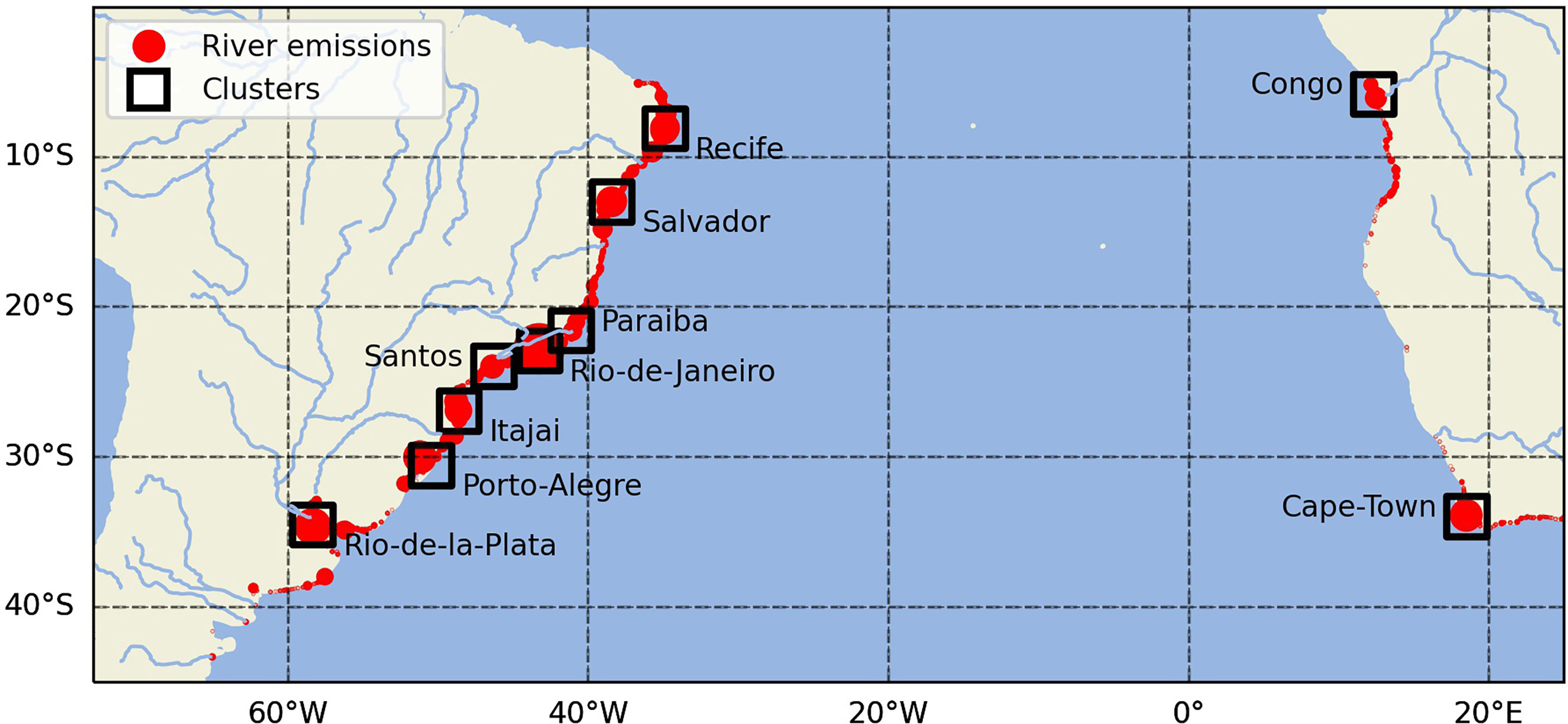
Figure 1 Map of the top plastic-emitting rivers (red dots) in the South Atlantic from Meijer et al. (2021) and the clusters (black squares) used as sources in this study. The size of the red circles is proportional to the rivers’ plastic emission. The size of the black squares exaggerates the true size of the clusters, which is 2° by 2°. The dots that fall outside the clusters represent the position for the river mouths of unclustered rivers on the American and African coast.

We defined the prior distribution p(R_i) to be the fraction of plastic emitted at each cluster, normalised by the total amount of plastic emitted at the 12 clusters. Our prior thus is a 12-dimensional categorical or discrete distribution, in which each source has an associated probability defined between 0 to 1, and the sum of the 12 probabilities is 1. The probability associated with each source is shown in Table 1.

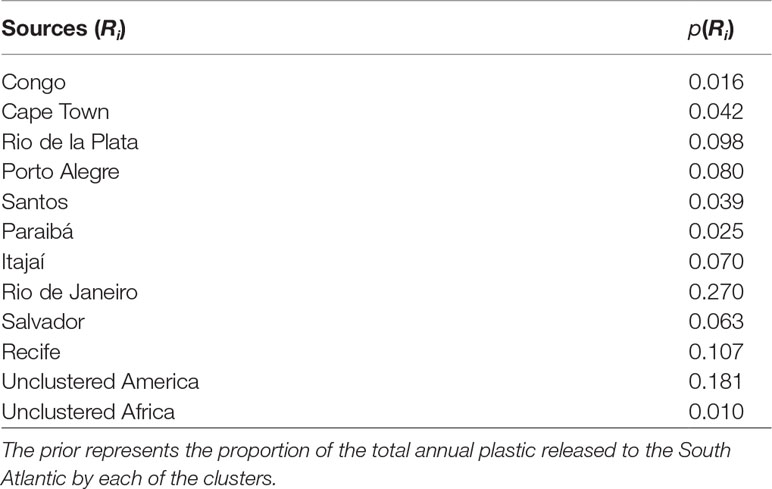
Table 1 Prior probability p(R_i) of floating plastic being released in a specific cluster R_i.

Numerical Simulation and Computing the Likelihood

To compute the likelihood p(S_loc|R_i) , we performed a forward in time Lagrangian simulation in which we released virtual particles from each of the clusters R_i and tracked them through the South Atlantic surface flow. We performed the simulation using the Parcels framework (Delandmeter and van Sebille, 2019) in combination with the Surface and Merged Ocean Currents (SMOC) hydrodynamic data from the Copernicus Marine Environmental Service (CMEMS). In particular, The SMOC data set is a 2D surface flow field, with a 1/12° resolution, of the sum of the velocity contributions from the Navier-Stokes currents from the 1/12° Nucleus for European Modeling of the Ocean [NEMO, Madec et al. (2017)], the tidal component from the FES2014 tidal model (Carrere et al., 2015), and the Stokes Drift component from the MétéoFrance Wave Action Model [MFWAM, Ardhuin et al. (2010)], each of these models by itself are extensively validated. Additionally, the SMOC have been used in similar studies such as Van Sebille et al. (2021) where they compared trajectories advected with SMOC and compared them to drifter data in the Tropical Atlantic. In this study we used the sum of three components of the SMOC and we assumed that the particles were at the surface at all times.

We performed one simulation per cluster, with 100,000 particles each, using a fourth-order Runge-Kutta integration time step of 1 h. For each simulation, we released the particles from the river mouth locations within the cluster. The number of particles released at each river mouth was proportional to the emission of each of the rivers within the cluster. In the simulations for the unclustered rivers, we released the particles from the river mouth locations outside the clusters. The number of particles released was proportional to the plastic emissions of each unclustered river. We released the particles continuously. The date of release of the particles was randomly selected from a uniform distribution over a time interval of one year. On average, the particles were released 10 km from the coast, or at the centers of the closest cell next to the river. We stored the particles’ positions every 24 h, for a total of 1,234 points per trajectory (3.4 years).

The domain of the simulation was the South Atlantic Ocean, from 70°W to 25°E and between 50°S to the Equator. We stopped tracking the particles if they exited the domain. In total, 16.2% of the particles exited the domain: 12.8% across the Equator and 3.4% into the Indian Ocean. We used hydrodynamic data from 1 April 2016 to 31 August 2020, releasing particles in the first year only and then tracking them for another 3.4 years. We selected these periods because the main objective of this study is to demonstrate the method with computationally feasible time scales, although they are small compared to plastic degradation time scales.

In the simulations, we implemented a stochastic parametrization for beaching of buoyant particles as described in Onink et al. (2021), using a characteristic beaching timescale of λ_b=10 days and a characteristic re-suspension timescale of λ_b=69 days. The λ_b is the beaching e-folding timescale, i.e. the amount of days that a particle has spent in the beaching zone to have a 63.2% chance of beaching. Similarly, λ_r is the resuspension e-folding timescale, the amount of days that a particle has to spend beached to have a chance of 63.2% to resuspend. We selected λ_r=69 days, within the validity range reported by Onink et al. (2021). We also performed another simulation using a λ_r=171 days. We found that the result and conclusion were consistent for both cases. The comparison from both results can be found in Text S1 and the results from the simulations with λ_r=171 days are shown in Figures S1–S4, in the Supplementary Information.

To parametrise unresolved turbulence that acts on the floating plastic (Van Sebille et al., 2020), we implemented uniform diffusion defined in the whole domain with a value of 10 m²s^–1, similar to Onink et al. (2021) and Lacerda et al. (2019).

We computed the likelihood p(S_loc|R_i) by binning the particle positions in 1 °× 1° bins. For this, we counted the particles inside each bin at every time step, and then we averaged the number of particles during a time window. Then, we divided the average number of particles at each bin by the sum of all the averaged counts in all bins, resulting in time-averaged likelihood. By using this time-averaged likelihood and eq. 5, we can obtain the time-averaged posterior probability, which describes the mean behavior of the posterior probabilities by removing temporal fluctuations. The resulting p(S_loc|R_i) in each bin has a value between 0 and 1 and the sum of the probabilities of all bins is 1. This yielded twelve p(S_loc|R_i) maps, one per source R_i.

The likelihood was computed based on the positions of the particles according to their age. The particle age represents the transit time of particles between the source R_i and a sampling location S_loc (i.e., their drifting time), with each particle following a different pathway until reaching S_loc (van Sebille et al., 2018).

Oceanic Particles Posterior Probability

We computed the posterior probability p(R_i|S_loc) using eq. (5) independently for each 1° by 1° bin, using the corresponding likelihood and the normalizing constant in each particular bin. Doing this for all the clusters, we get the local posterior distribution in each bin, as a probability between 0 and 1 for each source. This results in 12 posterior probability maps (one per cluster) which add up to 1 for each bin. Additionally, we computed the standard deviation of the posterior probability by performing a bootstrapping as explained in Text S2 in the Supplementary Information.

Beached Particles Posterior Probability

Since we use a stochastic parametrization for simulating the beaching of particles near the coast, we can also map the probability of a beached particle coming from a specific cluster. To compute this, we built two cumulative latitudinal histograms of the particles that were beached at a specific time step: one for the American coast and the other for the African coast. The cumulative latitudinal histogram is formed by counting the particles that are beached in latitudinal bins of 1°, disregarding the longitude of those particles, and by classifying them into particles that beached either at the American or the African coast. With the counts per latitude, we computed the average at each bin for the duration of the whole simulation and normalized by the sum of all average counts per bin. As for the posterior probability maps, we computed the beached posterior probability p(R_i|S_lat) using eq. (5), where S_lat is the latitudinal bin.

Results

Likelihood Maps

Figure 2 shows the likelihood maps for particles released at each cluster R_i , averaged over a period of 3.4 years. The values for the likelihood in the bins are between 0 to 10^–4, as they represent the proportion of particles (in relation to the total number of particles from a cluster in the domain) that cross a grid cell. Each cluster has 100,000 particles, minus the particles that exited the domain at a certain time step, so if in one bin there are 100 particles, the likelihood would be in the order of 10^–4.

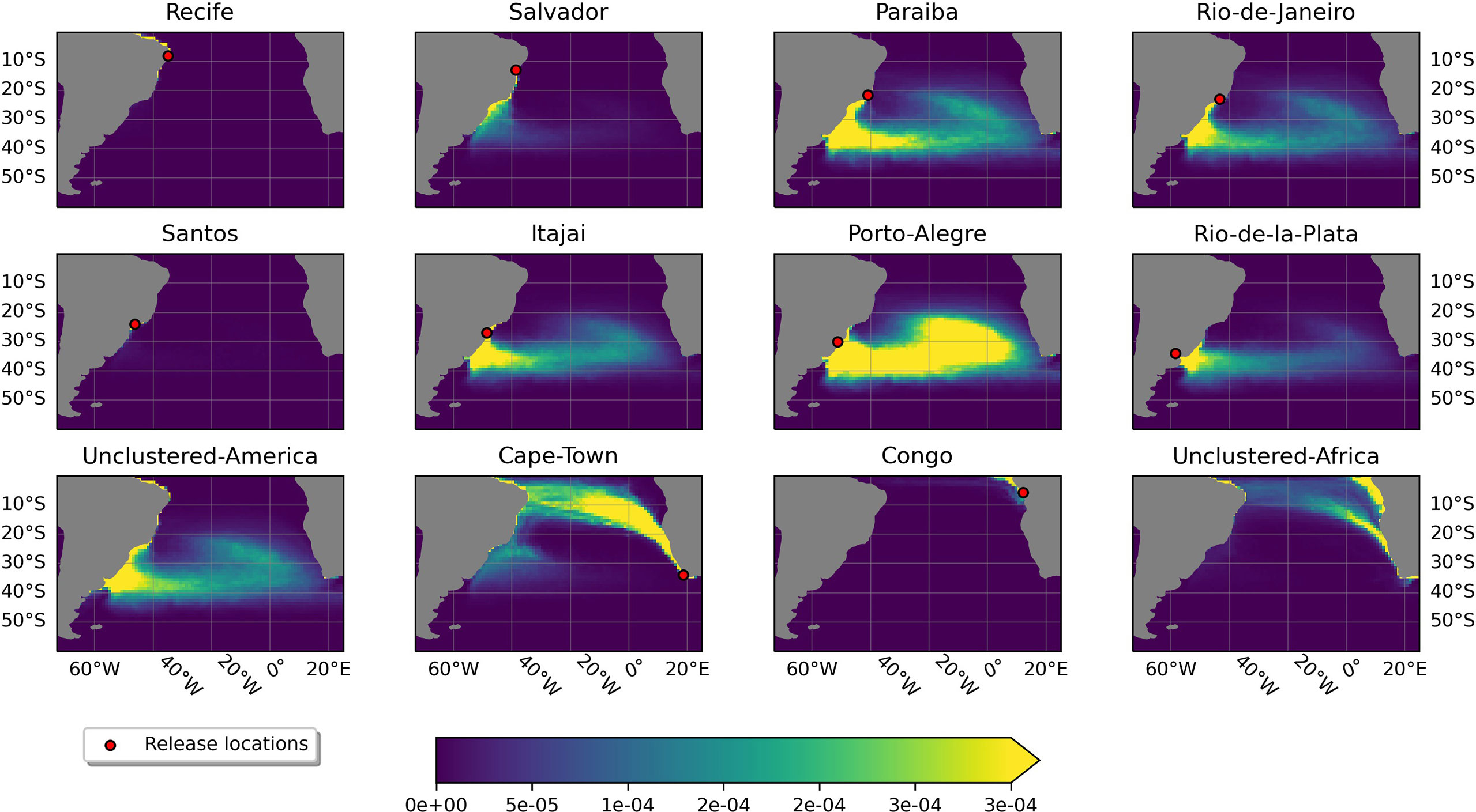
Figure 2 Likelihood maps of the spatially binned p(S_loc|R_i) for each cluster. The color scale indicates the probability of finding a plastic particle coming from the cluster, indicated as a red point.

In general, the dark blue areas represent regions where almost no particles were found from a specific cluster, while the yellow regions represent locations where it was more likely to find particles from that cluster. Specifically, for the South American clusters, the likelihood of finding particles from Recife, Santos, and Salvador is almost zero in the open ocean between 20°S to 40°S, that is, where the subtropical gyre is located. The particles released from those clusters tend to stay close to shore and beach because of the effect of Stokes drift that pushes them towards the coast.

The major contributors to the subtropical gyre plastic content (between 20°S to 40°S) are Itajaí, Paraíba, Porto Alegre, Rio de Janeiro, Rio de la Plata, and Unclustered-America, with likelihoods ranging from 1 x 10^–4 to 10^–4. From these clusters, Porto Alegre is the largest contributor. Closer to the South American coast, the likelihood is above 3 x 10^–4 for all these clusters. North of the gyre, from 20°S and further north, the likelihood of finding particles from the American coast is near-zero.

For the African clusters, shown on Figure 2, we see that the likelihood of finding particles released in Cape Town is the highest in the Benguela Current (refer to Bower et al. (2019) for a schematic of the Atlantic features and currents). These particles are likely to reach the South American coast near the Cape of Saõ Roque, and will less likely get carried by the Brazil Current towards the coast of Argentina. The particles released at the Congo get carried away northward to the Equator, outside of the domain of our simulation, and are unlikely to be found in other parts of the domain. For Unclustered-Africa, we can see that the likelihood is high along the Benguela current and on the Angolan coast.

Oceanic Particles Posterior Probability

Figure 3 shows the posterior probability p(R_i|S_loc) maps for each cluster, averaged over 3.4 years. In particular, the particles in our simulation do not reach latitudes south of 50°S, leading to no defined posterior probability in the Antarctic Circumpolar Current (ACC). This is due to the generally northward Ekman drift in the ACC (Onink et al., 2019), and because we assumed that the particles only originate from twelve clusters placed north of 50°S.

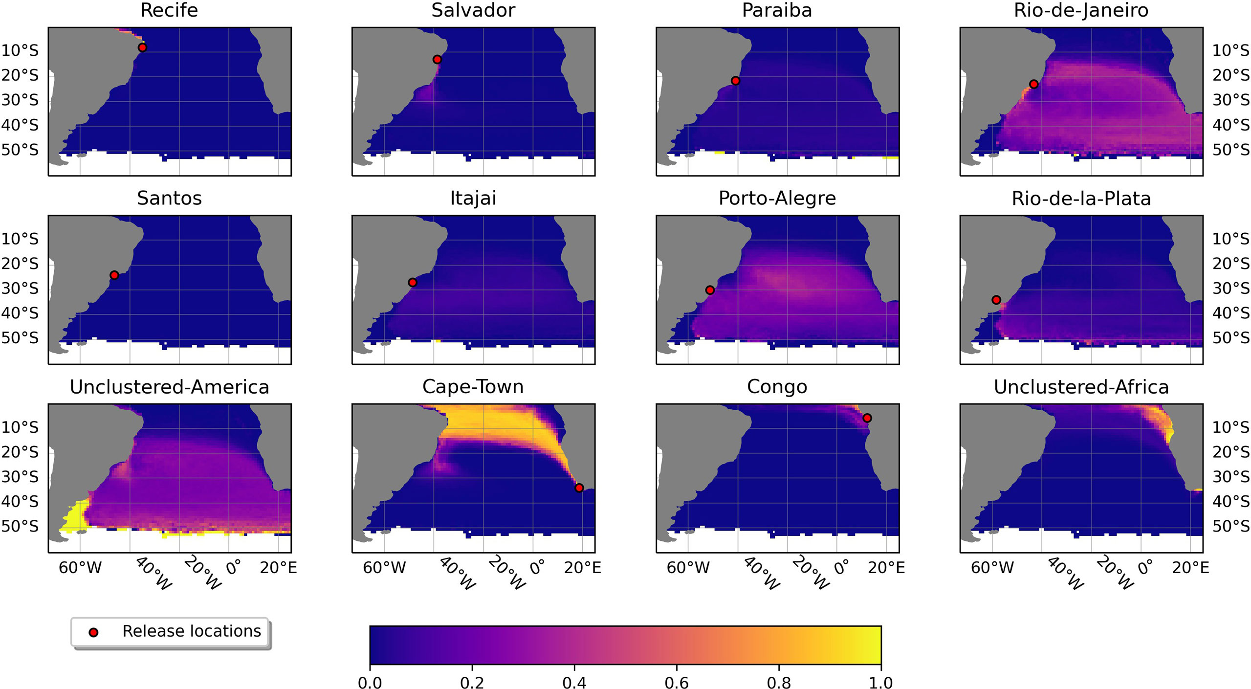
Figure 3 Posterior probability maps, averaged over 3.4 years, showing p(R_i|S_loc), the probability of finding a particle from a specific cluster at any point in the South Atlantic. Each map displays the probability for a specific cluster in all the bins of the domain. The red dots indicate the locations of the clusters from which the particles entered the ocean. At each location, the sum of posterior probability of the twelve clusters is 1.

Regarding the individual panels in Figure 3, the three clusters that dominate in the region of the subtropical gyre, between 20°S to 50°S, are Porto Alegre, Rio de Janeiro, and Unclustered-America, with probabilities around 30%. The posterior probabilities for Recife and Santos are near-zero because only very few particles were transported into the open ocean. The probability that particles end up between 50°W to 40°W and close to Brazil originated from Salvador is up to 30%. The posterior probabilities of Itajaí and Paraíba are below 10% everywhere. At the boundary with the ACC, the source with the largest probability is the Unclustered-American rivers, followed by Rio de Janeiro and Rio de la Plata. South of South Africa, particles released from Rio de Janeiro and the Unclustered-American rivers are dominant, with 40% and 30% respectively. The remaining 30% are mainly contributed by Porto Alegre and Rio de la Plata. In the Benguela Current region until the northern coast of Brazil, the probability is dominated by the Cape Town cluster (close to 100%). The Unclustered-African cluster has the largest probabilities from 20°S towards the equator, with probabilities close to 100% near the coast. Finally, the posterior probability of the Congo cluster is almost only appreciable near the source and farther north.

Local Posterior Age Distributions

The posterior age distributions yield the probable sources of a particle of a certain age, sampled at a certain location. Figure 4 shows the posterior age distributions for three sampling locations, averaged over a time window of 30 days, to smooth variations at sub-monthly time-scales. The color shading represent the standard deviation associated with the probability of each cluster. The dashed line represents the number (N ) of particles that reach the location as a function of age. The posterior probability distributions were only computed when N>10. Location B matches the location where samples were collected in a 2019 expedition (Weckhuysen et al., 2021) and we selected the sampling locations A and C as representative of the rest of the gyre circulation.

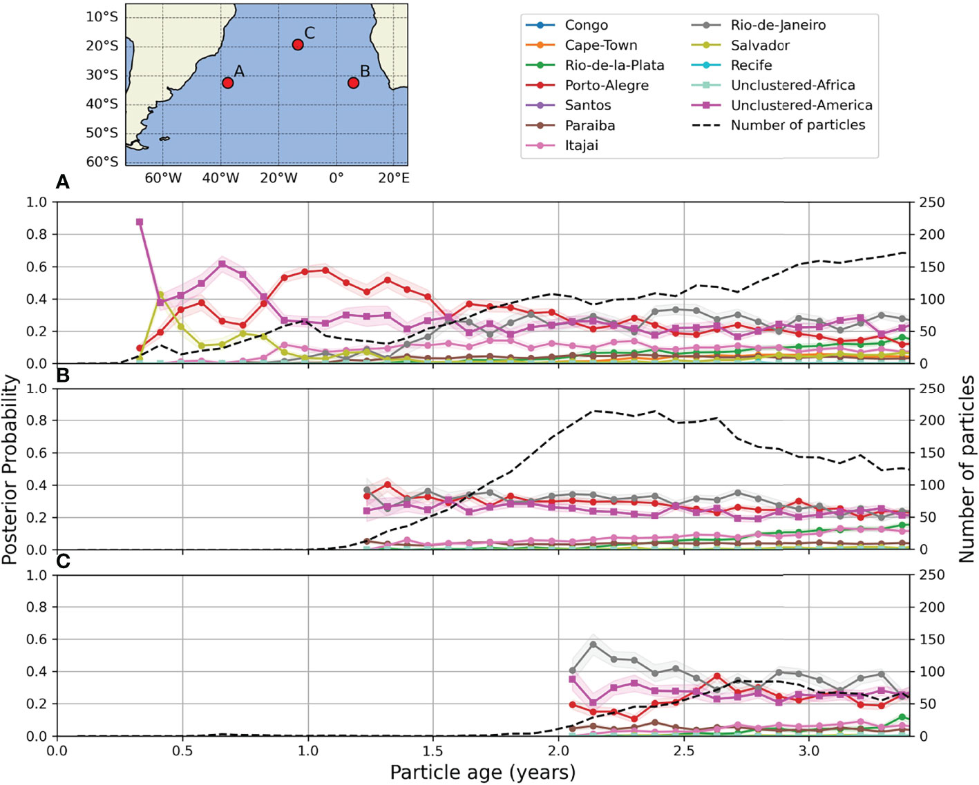
Figure 4 Local posterior age distributions at three different locations for the posterior probability. The map on the top right marks the locations (A−C), that correspond to the time series shown in the plots (A−C). Each color in (A−C), represents the probability p(R_i|S_loc) for a particular cluster. The color shading shows the standard deviation associated with the probabilities. The black dashed line represents the number of particles (N ) at the respective location.

The panel for sampling location A in Figure 4, located in the western part of the subtropical gyre (32.37°S, 37.64°W), shows for example that a particle sampled at that location with age younger than 0.4 years is very unlikely to come from any of the considered river clusters. For particles between 0.4 years to 1.0 years, the most probable sources are Unclustered-America, Salvador and Porto Alegre. For ages older than 1.0 years, the probability from Unclustered-America drops below 40%, Salvador drops below 10% while Porto Alegre remains stable. For particles older than 1.5 years, the probabilities asymptote towards approximately time-constant values: Porto Alegre, Rio de Janeiro, and Unclustered-America have the largest probabilities, with values fluctuating between 20% and 40%. The rest of the clusters have values below 20%.

The posterior age distributions for location B (32.37°S, 5.80°E) in Figure 4, show that it is unlikely to find particles younger than 1.2 years coming from any of the considered clusters: only particles older than 1.4 years can reach this point. Similar to point A, the clusters with the largest probability, throughout all ages, are Rio de Janeiro, Porto Alegre and Unclustered-America. For the younger particles, these probabilities oscillate around 30%, while for older particles, the three clusters decrease down to 20% for 3.4-year-old particles. The remaining clusters stay below 20% for all ages. The plot corresponding to point C located north of the gyre (19.19°S, 13.39°W), shows that particles reach this location two years after release. Fewer particles were present on average compared to A and B, reaching a peak N at 2.7 years. The largest probability corresponds to Rio de Janeiro, followed by Unclustered-America, and Porto Alegre. The other clusters remain below 10% for all ages recorded.

Beached Particles Posterior Probability

Figure 5 shows the posterior probabilities for a particle to beach at certain latitude, p(R_i|S_lat) , based on its origin. The p(R_i|S_lat) for the American coast are displayed in the left panel and the ones for the African coast are shown in the right panel. On the American coast, the nearest cluster to the bin S_lat has the highest probability, which peaks at the same latitude as the cluster or in its vicinity. This suggests that the plastic found on beaches close to a source is most likely to come from that source. Santos is the only exception to this trend because its probability is overshadowed by its proximity to Rio de Janeiro which emissions are six times larger. The Unclustered-American rivers dominate the latitudes where there are no clusters present such as between 15°S to 21°S and South of 38°S.

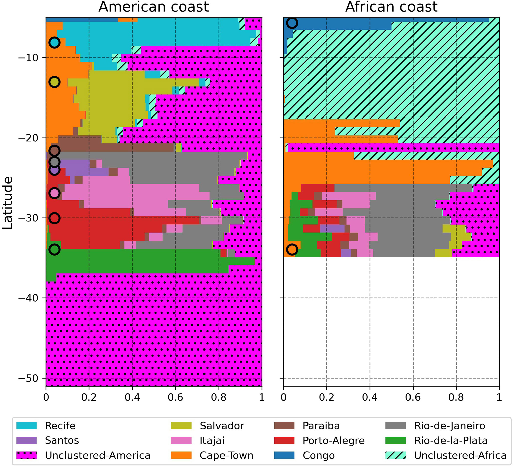
Figure 5 Horizontal bar plot for the posterior probabilities of beached particles (x -axis) at a specific latitude (y -axis). The panel on the left shows the probabilities at the American Coast and the panel on the right the probabilities at the African coasts. Each color is associated with a cluster, shown in the legend at the bottom. Each latitude has a corresponding horizontal bar summing the probabilities from the clusters at that latitude to 1. The round markers on the left of each plot represent the latitudes of the clusters. If the marker is on the left panel, the cluster is at the American coast, and if the marker is in the right panel, the cluster is located at the African coast.

In the right panel of Figure 5, the beached probabilities for latitudes between 25°S to 35°S on the African coastline show a dominance of particles coming from the American coast, accounting for more than 90% of the beached particles. The probability of the beached particles coming from Cape Town is less than 10% in this region. This is because the particles from the American clusters have higher prior probability than the plastic from the African clusters. Between 23°S to 25°S, Cape town is dominant for beached particles. In the region between 7°S to 19°S, the Unclustered-Africa cluster dominates, mainly due to the absence of other river clusters. Finally, at 5°S latitude, the most probable cluster was Congo.

Discussion and Conclusions

We introduced a Bayesian probabilistic framework that estimates p(R_i|S_loc) , the probability that a plastic particle, sampled at the surface of the South Atlantic Ocean, came from a particular river cluster, as a use case example. The novelty of this framework is that it performs a forward in time Lagrangian simulation from the defined sources. This approach has the advantage of using only one Lagrangian simulation, while in a backward in time Lagrangian simulation we would have to perform a simulation per sampling location.

The framework supports different types of analyses and can be used, for example, to compute spatial probabilities, compute the local probability as a function of particle age, or analyse the probabilities once a physical process (e.g. beaching) alters the particles’ state. We applied this method to the use case of plastic emitted at river mouths in the South Atlantic. This application ignores other types of sources that also contribute to marine plastic pollution, such as fisheries, cities, or plastic from outside the domain; and thus make it difficult to validate these results with direct observations. Nevertheless, the framework could in principle be extended to other types of sources.

The time average window used for computing the likelihood p(S_loc|R_i) can be adjusted according to the aim of the study. Usually, computing the likelihood for small time windows leads to greater variability in the likelihood and for instance in the posterior probability. For these reasons, we computed the average likelihood for the whole simulation (3.4 years), and from there we computed the posterior probability.

As we showed in Figure 3, visualizing the posterior p(R_i|S_loc) in maps allows us to identify the most important clusters that pollute ocean regions that provide high ecosystem services and that are vulnerable to plastic, such as subtropical gyres (Helm, 2021) and marine protected areas (Krüger et al., 2017). This can be used to prioritize the reduction of MPW in the principal sources to mitigate the problem. For example, our use case showed that Porto Alegre, Rio de Janeiro and Unclustered-America are the most probable sources of local riverine plastic in the South Atlantic Subtropical Gyre.

The local posterior age distributions, shown in Figure 4 further illustrate the analysis that can be done by selecting a location and by computing the probability distributions as a function of the particle’s age. This can point to the most likely source if we estimate the time the plastic has been drifting in the ocean, by assessing its degradation (Gewert et al., 2015; Chamas et al., 2020). Moreover, we observed that after 3 years the posterior age probability asymptote towards constant values, which suggests that for longer simulation times, the probabilities will remain relatively constant in time.

The latitudinal beached posterior probabilities, shown in Figure 5, demonstrate how this framework can be used to analyse the contribution of different sources to particle sinks (e.g. beaches) when considering certain physical processes that alter particle pathways (e.g. the process of beaching). This can be expanded by including other additional physical processes that can alter the dynamical state of the virtual particles, such as sinking (Lobelle et al., 2021; Fischer et al., 2022), directly in the simulations. The framework is independent of the physical processes that affect plastic. Adding to the limitations of this framework, it does not allow us to identify the physical processes responsible for the transport of plastic in the ocean.

In our use case on floating plastic emitted from rivers in the South Atlantic, we ignore plastic entering the domain from the Indian Ocean leakage (Van der Mheen et al., 2019) and from the North Atlantic (Speich et al., 2007). To consider it, these leakages could for example be assumed as sources, by knowing how much plastic enters the domain through the boundaries, or the domain could be extended to consider other basins.

One major advantage of the Bayesian nature of our framework is that it allows updating the results when better estimates of plastic emissions are available without having to redo the (computationally expensive) Lagrangian simulations. For instance, it can be expanded by including a prior that accounts for seasonal variations in river-borne plastic inputs, or by taking into account different types of land-based or sea-based sources. Also, the forward simulation releases the same amount of particles per cluster or source, which makes small emitting sources have equal spatial representation compared to larger and more dominant sources.

Data Availability Statement

The original contributions presented in the study are publicly available. This data can be found here: https://doi.org/10.24416/UU01-THF29M.

Author Contributions

CP, DB, and ES contributed to the conceptualization and design of this study. CP performed the simulations and the analysis, and wrote the original draft. BD, FM, ES contributed to the editing of the original draft. All authors contributed to manuscript revision, read, and approved the submitted version.

Funding

This project was supported by NWO through grant OCENW.GROOT.2019.043. EvS was partly supported through funding from the European Research Council (ERC) under the European Union’s Horizon 2020 research and innovation programme (grant agreement No 715386).

Conflict of Interest

The authors declare that the research was conducted in the absence of any commercial or financial relationships that could be construed as a potential conflict of interest.

Publisher’s Note

All claims expressed in this article are solely those of the authors and do not necessarily represent those of their affiliated organizations, or those of the publisher, the editors and the reviewers. Any product that may be evaluated in this article, or claim that may be made by its manufacturer, is not guaranteed or endorsed by the publisher.

Supplementary Material

The Supplementary Material for this article can be found online at https://www.frontiersin.org/articles/10.3389/fmars.2022.925437/full#supplementary-material

References

Ardhuin F., Rogers E., Babanin A. V., Filipot J.-F., Magne R., Roland A., et al. (2010). Semiempirical Dissipation Source Functions for Ocean Waves. Part I: Definition, Calibration, and Validation. J. Phys. Oceanogr. 40, 1917–1941. doi: 10.1175/2010JPO4324.1
Bower A., Lozier S., Biastoch A., Drouin K., Foukal N., Furey H., et al. (2019). Lagrangian Views of the Pathways of the Atlantic Meridional Overturning Circulation. J. Geophys. Res.: Oceans. 124, 5313–5335. doi: 10.1029/2019JC015014
Carrere L., Lyard F., Cancet M., Guillot A. (2015). “Fes 2014, a New Tidal Model on the Global Ocean With Enhanced Accuracy in Shallow Seas and in the Arctic Region,” in EGU General Assembly Conference Abstracts(Austria: EGU General Assembly), 5481.
Chamas A., Moon H., Zheng J., Qiu Y., Tabassum T., Jang J. H., et al. (2020). Degradation Rates of Plastics in the Environment Vol. 8 (Washington DC; USA: ACS Sustainable Chemistry & Engineering), 3494–3511.
Cózar A., Echevarría F., González-Gordillo J. I., Irigoien X., Úbeda B., Hernández-León S., et al. (2014). Plastic Debris in the Open Ocean. Proc. Natl. Acad. Sci. 111, 10239–10244. doi: 10.1073/pnas.1314705111
Davey S., Gordon N., Holland I., Rutten M., Williams J. (2016). Bayesian Methods in the Search for MH370 (Singapore: Springer Nature).
Delandmeter P., van Sebille E. (2019). The Parcels V2. 0 Lagrangian Framework: New Field Interpolation Schemes. Geoscientific. Model. Dev. 12, 3571–3584. doi: 10.5194/gmd-12-3571-2019
do Sul J. A. I., Costa M. F. (2007). Marine Debris Review for Latin America and the Wider Caribbean Region: From the 1970s Until Now, and Where Do We Go From Here? Mar. Pollut. Bull. 54, 1087–1104. doi: 10.1016/j.marpolbul.2007.05.004
Eriksen M., Lebreton L. C., Carson H. S., Thiel M., Moore C. J., Borerro J. C., et al. (2014). Plastic Pollution in the World’s Oceans: More Than 5 Trillion Plastic Pieces Weighing Over 250,000 Tons Afloat at Sea. PLoS One 9, e111913. doi: 10.1371/journal.pone.0111913
Fischer R., Lobelle D., Kooi M., Koelmans A., Onink V., Laufkötter C., et al. (2022). Modelling Submerged Biofouled Microplastics and Their Vertical Trajectories. Biogeosciences 19, 2211–2234. doi: 10.5194/bg-19-2211-2022
Gewert B., Plassmann M. M., MacLeod M. (2015). Pathways for Degradation of Plastic Polymers Floating in the Marine Environment. Environ. Sci.: Processes. Impacts. 17, 1513–1521. doi: 10.1039/C5EM00207A
Hardesty B. D., Harari J., Isobe A., Lebreton L., Maximenko N., Potemra J., et al. (2017). Using Numerical Model Simulations to Improve the Understanding of Micro-Plastic Distribution and Pathways in the Marine Environment. Front. Mar. Sci. 4, 30. doi: 10.3389/fmars.2017.00030
Helm R. R. (2021). The Mysterious Ecosystem at the Ocean’s Surface. PloS Biol. 19, e3001046. doi: 10.1371/journal.pbio.3001046
Jambeck J. R., Geyer R., Wilcox C., Siegler T. R., Perryman M., Andrady A., et al. (2015). Plastic Waste Inputs From Land Into the Ocean. Science 347, 768–771. doi: 10.1126/science.1260352
Jambeck J., Hardesty B. D., Brooks A. L., Friend T., Teleki K., Fabres J., et al. (2018). Challenges and Emerging Solutions to the Land-Based Plastic Waste Issue in Africa. Mar. Policy 96, 256–263. doi: 10.1016/j.marpol.2017.10.041
Koelmans B., Pahl S., Backhaus T., Bessa F., van Calster G., Contzen N., et al. (2019). A Scientific Perspective on Microplastics in Nature and Society (SAPEA) Water Res 155, 410-422. doi:10.1016/j.watres.2019.02.054
Krüger L., Ramos J., Xavier J., Grémillet D., González-Solís J., Kolbeinsson Y., et al. (2017). Identification of Candidate Pelagic Marine Protected Areas Through a Seabird Seasonal-, Multispecific-and Extinction Risk-Based Approach. Anim. Conserv. 20, 409–424. doi: 10.1111/acv.12339
Lacerda A.L.d. F., Rodrigues L., Van Sebille E., Rodrigues F. L., Ribeiro L., Secchi E. R., et al. (2019). Plastics in Sea Surface Waters Around the Antarctic Peninsula. Sci. Rep. 9, 1–12. doi: 10.1038/s41598-019-40311-4
Lebreton L., Andrady A. (2019). Future Scenarios of Global Plastic Waste Generation and Disposal. Palgrave. Commun. 5, 1–11.doi:10.1057/s41599-018-0212-7
Lebreton L., Slat B., Ferrari F., Sainte-Rose B., Aitken J., Marthouse R., et al. (2018). Evidence That the Great Pacific Garbage Patch Is Rapidly Accumulating Plastic. Sci. Rep. 8, 1–15. doi: 10.1038/s41598-018-22939-w
Lobelle D., Kooi M., Koelmans A. A., Laufkötter C., Jongedijk C. E., Kehl C., et al. (2021). Global Modeled Sinking Characteristics of Biofouled Microplastic. J. Geophys. Res.: Oceans. 126, e2020JC017098. doi: 10.1029/2020JC017098
Madec G., Bourdallé-Badie R., Bouttier P.-A., Bricaud C., Bruciaferri D., Calvert D., et al. (2017). Nemo Ocean Engine .Guyancour: Institut Pierre-Simon Laplace (IPSL)
Meijer L. J., van Emmerik T., van der Ent R., Schmidt C., Lebreton L. (2021). More Than 1000 Rivers Account for 80% of Global Riverine Plastic Emissions Into the Ocean. Sci. Adv. 7, eaaz5803. doi: 10.1126/sciadv.aaz5803
Morris R. J. (1980). Plastic Debris in the Surface Waters of the South Atlantic. Mar. Pollut. Bull. 11, 164–166. doi: 10.1016/0025-326X(80)90144-7
Onink V., Jongedijk C., Hoffman M., van Sebille E., Laufkötter C. (2021). Global Simulations of Marine Plastic Transport Show Plastic Trapping in Coastal Zones. Environ. Res. Lett. 16, 6, doi: 10.1088/1748-9326/abecbd
Onink V., Wichmann D., Delandmeter P., van Sebille E. (2019). The Role of Ekman Currents, Geostrophy, and Stokes Drift in the Accumulation of Floating Microplastic. J. Geophys. Res.: Oceans. 124, 1474–1490. doi: 10.1029/2018JC014547
Richardson H. R., Stone L. D.,(1971). Operations Analysis During the Underwater Search for Scorpion. Naval. Res. Logistics. Q. 18, 141–157. doi: 10.1002/nav.3800180202
Ryan P. G. (2014). Litter Survey Detects the South Atlantic ‘Garbage Patch’. Mar. Pollut. Bull. 79, 220–224. doi: 10.1016/j.marpolbul.2013.12.010
Schofield J., Wyles K. J., Doherty S., Donnelly A., Jones J., Porter A. (2020). Object Narratives as a Methodology for Mitigating Marine Plastic Pollution: Multidisciplinary Investigations in Galapagos. Antiquity 94, 228–244. doi: 10.15184/aqy.2019.232
Speich S., Blanke B., Cai W. (2007). Atlantic Meridional Overturning Circulation and the Southern Hemisphere Supergyre. Geophys. Res. Lett. 34(13), L23614. doi: 10.1029/2007GL031583
Turner A., Williams T., Pitchford T. (2021). Transport, Weathering and Pollution of Plastic From Container Losses at Sea: Observations From a Spillage of Inkjet Cartridges in the North Atlantic Ocean. Environ. Pollut. 284, 117131. doi: 10.1016/j.envpol.2021.117131
Van der Mheen M., Pattiaratchi C., van Sebille E. (2019). Role of Indian Ocean Dynamics on Accumulation of Buoyant Debris. J. Geophys. Res.: Oceans. 124, 2571–2590. doi: 10.1029/2018JC014806
van Duinen B., Kaandorp M. L., van Sebille E. (2021). Identifying Marine Sources of Beached Plastics Through a Bayesian Framework: Application to Southwest Netherlands. Geophys. Res. Lett., 49 (4), e2021GL097214. doi: 10.1029/2021GL097214
Van Sebille E., Aliani S., Law K. L., Maximenko N., Alsina J. M., Bagaev A., et al. (2020). The Physical Oceanography of the Transport of Floating Marine Debris. Environ. Res. Lett. 15, 023003. doi: 10.1088/1748-9326/ab6d7d
van Sebille E., Griffies S. M., Abernathey R., Adams T. P., Berloff P., Biastoch A., et al. (2018). Lagrangian Ocean Analysis: Fundamentals and Practices. Ocean. Model. 121, 49–75. doi: 10.1016/j.ocemod.2017.11.008
Van Sebille E., Wilcox C., Lebreton L., Maximenko N., Hardesty B. D., Van Franeker J. A., et al. (2015). A Global Inventory of Small Floating Plastic Debris. Environ. Res. Lett. 10, 124006. doi: 10.1088/1748-9326/10/12/124006
Van Sebille E., Zettler E., Wienders N., Amaral-Zettler L., Elipot S., Lumpkin R. (2021). Dispersion of Surface Drifters in the Tropical Atlantic. Front. Mar. Sci. 7, 1243. doi: 10.3389/fmars.2020.607426
Keywords: Bayesian inference, circulation, plastic, South Atlantic, Lagrangian
Citation: Pierard CM, Bassotto D, Meirer F and van Sebille E (2022) Attribution of Plastic Sources Using Bayesian Inference: Application to River-Sourced Floating Plastic in the South Atlantic Ocean. Front. Mar. Sci. 9:925437. doi: 10.3389/fmars.2022.925437
Received: 21 April 2022; Accepted: 06 June 2022;
Published: 14 July 2022.
Edited by:
Matteo Baini, University of Siena, ItalyReviewed by:
Carlo Brandini, CNR, ItalyShiye Zhao, Japan Agency for Marine-Earth Science and Technology (JAMSTEC) Japan
Copyright © 2022 Pierard, Bassotto, Meirer and van Sebille. This is an open-access article distributed under the terms of the Creative Commons Attribution License (CC BY). The use, distribution or reproduction in other forums is permitted, provided the original author(s) and the copyright owner(s) are credited and that the original publication in this journal is cited, in accordance with accepted academic practice. No use, distribution or reproduction is permitted which does not comply with these terms.
*Correspondence: Claudio M. Pierard, c.m.pierard@uu.nl