Acoustic Classification of Juvenile Pacific Salmon (Oncorhynchus spp) and Pacific Herring (Clupea pallasii) Schools Using Random Forests

Introduction

Acoustic surveys are commonly used to monitor fish and zooplankton in many parts of the world. These surveys can be conducted from a moving vessel (Johannesson and Mitson, 1983; Simmonds et al., 1991; Simmonds and MacLennan, 2005; Parker-Stetter et al., 2009) or from fixed platforms (Thomson and Allen, 2000; Kaartvedt et al., 2009; Sato et al., 2013). Acoustic surveys are an integral part of a number of fish stock management programs. Examples in Canada include the Pacific Hake joint stock assessment (Edwards et al., 2022), the Atlantic herring stock assessment in the northern Gulf of St. Lawrence (Chamberland et al., 2022), and the capelin stock assessment in Newfoundland (Bourne et al., 2021). In 2015, a project was initiated to monitor juvenile Pacific salmon during their northward out-migration to reach the Pacific Ocean from the Strait of Georgia through the Discovery Islands and Johnstone Strait. Several fixed, upward looking echosounders were deployed in small bays in order to track the migration timing and relative abundance of juvenile Pacific salmon through the area (Rousseau et al., 2018). The Discovery Islands archipelago has been characterized as a high nutrient low chlorophyll (HNLC) region limited by light availability, and has been suggested to constitute a bottleneck region for juvenile Pacific salmon due to reduced food availability (Mckinnell et al., 2014). Pacific herring is also common in the area (Haegele et al., 2005).

The study involved the recording of several months of acoustic data each year, and a need emerged for replicable, automated methods of data processing and classification. The identification and classification of fish species is an ever-existing challenge in fisheries acoustics research. In many cases, acoustic targets are classified through “expert scrutiny”, based on information gathered from various means of validation sampling such as pelagic trawl, seine, and underwater video cameras, as well as prior knowledge on the frequency response, schooling behavior and typical habitat of each species. In addition to being highly time-consuming, this method involves a significant level of subjectivity as it relies heavily on the analyst’s knowledge and experience, and each validation method is subject to its own bias (McClathie et al., 2000; Fernandes, 2009; Boldt et al., 2019).

In recent years, efforts have been undertaken to automate part or all of the acoustic classification process in order to improve accuracy and replicability. Multi-frequency analysis can provide a way to increase objectivity and has been used successfully to differentiate krill from fish (Watkins and Brierley, 2002; De Robertis et al., 2010). However, when applied to more similar species, such as fish with a swim bladder or similar size classes of zooplankton, the success of this technique is often limited by the overlap in their frequency-response (Lavery et al., 2007; Gauthier et al., 2014; Sato et al., 2015). Several attempts have been made to improve the classification process by the introduction of multiple predictors, such as combining acoustic response with morphological characteristics of the aggregations using linear statistical models (Lawson et al., 2001; Woodd-Walker et al., 2003), and obtained promising results. More recently, several studies have explored machine learning methods such as neural networks and random forests as a way to integrate acoustic frequency response and school shape characteristics to automate and improve classification (Cabreira et al., 2009; Fallon et al., 2016; Brautaset et al., 2020; Proud et al., 2020).In this study, we used acoustic data from one of the autonomous echosounders deployed in the Discovery Islands, British Columbia to evaluate the use of a random forest classifier to distinguish juvenile Pacific salmon (Oncorhynchus spp) from Pacific herring (Clupea pallasii) aggregations using their acoustic response and the morphological characteristics of their echo traces. We developed a training dataset using acoustic data classified through expert scrutiny informed by net-based fish sampling from a purse seining program, a high-resolution imaging sonar, and prior knowledge from extensive herring survey monitoring programs in the Strait of Georgia and the west coast of Vancouver Island.

Materials and Methods

Data Sources

As part of a larger study aiming to better understand the early marine survival of juvenile Pacific salmon in the coastal waters of British Columbia, several autonomous, single-beam echosounders (Acoustic Zooplankton and Fish Profiler (AZFP), ASL Environmental Sciences) were deployed in the Discovery Islands between 2015 and 2020. The instruments were deployed on the seafloor looking upward. This enabled us to continuously monitor the relative abundance, distribution, and behavior of juvenile salmon through the area (Rousseau et al., 2018). In the lower mainland of British Columbia, a large number of rivers and streams, which support wild salmon populations, enter the Strait of Georgia, and the majority of juvenile salmon from these systems reach the Pacific Ocean by migrating north through the Discovery Islands and Johnstone Strait (Tucker et al., 2009; Beacham et al., 2014), a region located between the eastern side of central Vancouver Island and the British Columbia mainland (Figure 1). These areas are characterized by narrow restricted channels that have very high current velocities and often high wind conditions, and this often restricts the use of net-based surveys for juvenile salmon.

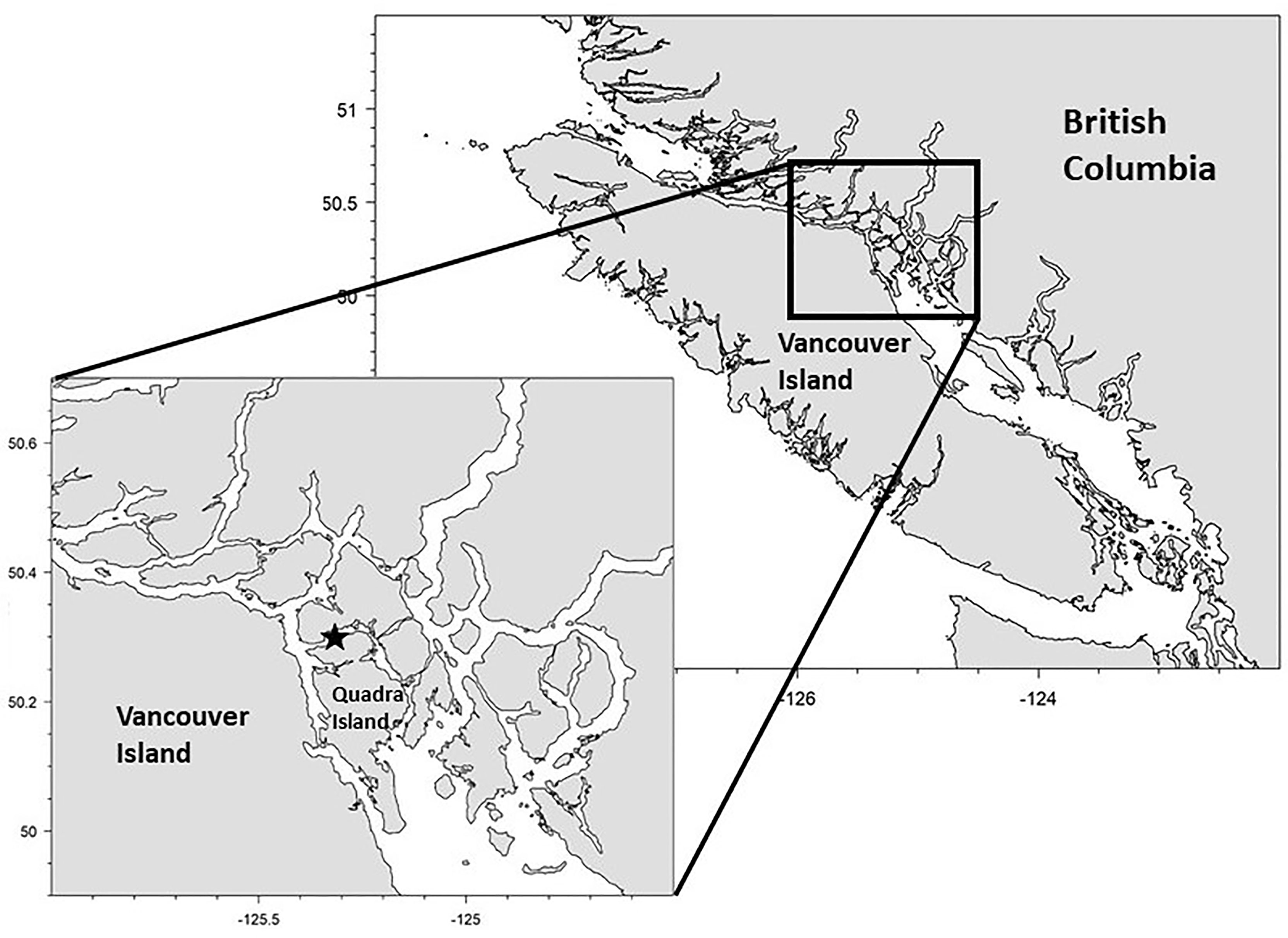
Figure 1 Location of AZFP mooring (black star) in the Discovery Islands, between Vancouver Island and the mainland of British Columbia

Data Collection

For the purposes of this study, we used data collected by one autonomous echosounder deployed in Okisollo Channel from May to September 2015. Okisollo Channel is a sheltered body of water separating the islands of Sonora and Quadra in the Discovery Islands, British Columbia (Figure 1). This site was the most accessible among all sites sampled, and in 2015 we were able to obtain bi-weekly fishing data and conduct bi-weekly high-resolution sonar surveys of the area during the expected migration window of juvenile salmon (Neville et al., 2016; Freshwater et al., 2019) to provide groudtruthing. The site was located in a small bay approximately 170 m from shore, at a bottom depth of 55 m. The echosounder operated at 4 frequencies (67, 125, 200, 455 kHz); however only the three lower frequencies were used in this study. The highest frequency (455 kHz) exhibited attenuation beyond our acceptable 10 dB signal to noise ratio at ranges greater than 30 meters. Each transducer was calibrated by ASL Environmental Sciences using a calibrated hydrophone and transmitter in a freshwater tank. Calibration checks using a 12.7 mm diameter tungsten-carbide sphere were carried out each year (before and after each deployment) to ensure that measured outputs were within 1 dB of the sphere’s theoretical value on or near axis.

A sampling interval of 3 s and a vertical sampling of 0.09 m were chosen as a compromise between data resolution, battery consumption and data storage space. A pulse duration of 500 µs was used at 67 kHz, and 300 µs was used for higher frequencies. A digitization rate of 64 kHz was used for all frequencies.Monthly average sound speed (Mackenzie, 1981) and absorption coefficient (Francois and Garrison, 1982) were calculated from temperature and salinity profiles collected between May and July 2015 (SBE-25 Sea-Bird Scientific). Monthly values for August and September were calculated from a linear interpolation of the May to July time series.Purse seine surveys were conducted twice a week from May 12 to July 15 in 2015 following the known presence of juvenile salmon in the area. Sampling was performed with a small mesh purse seine on a commercial seiner during slack and low flow tides (Neville et al., 2016; Freshwater et al., 2019). The seine was equipped with a bunt of 7 mm mesh designed to retain juvenile salmon and other small pelagics. Purse seining was carried out close to the acoustic mooring site, often within 200 m distance and on a few occasions directly on top of the mooring. As the seine sampled the top 20 m of the water column, it is likely that Pacific herring, which is often found deeper in the water column during day time (Thompson et al., 2016), was under-sampled compared to juvenile Pacific salmon. All species captured by the purse seiner were counted and identified (Table 1). Oncorhynchus spp and Clupea pallasii were the only fish species caught by the purse seine in the study area.Additional information on Pacific herring acoustic signature and school characteristics were obtained from midwater trawl-verified echograms collected on mobile acoustic surveys off coastal British Columbia. These data were collected from the CCGS W.E. Ricker operating a hull-mounted Simrad EK60 echosounder at 38 and 120 kHz (see Boldt et al., 2016 and Gauthier et al., 2016 for a general description of the main surveys). These surveys confirmed that Pacific herring was found at depth during the day and was identified as high-density and vertically elongated schools in the acoustic echograms. Boldt et al. (2019) provide information regarding the challenges of target validation in Pacific herring and other forage fish acoustic surveys.

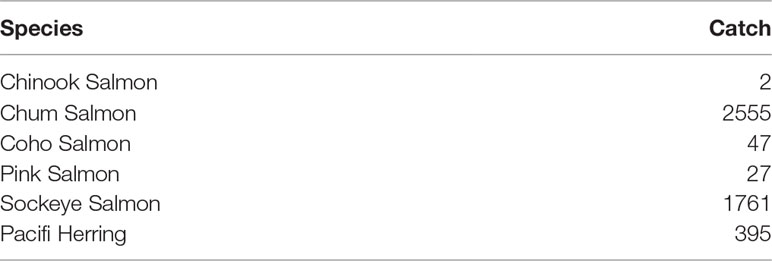
Table 1 Total number of juvenile Pacific salmon and Pacific herring individuals caught by the purse seiner in Okisollo Channel.

Small mobile surveys, using a vessel-mounted, side-looking imaging-sonar (Sound Metrics DIDSON), were also conducted in the area of the mooring and helped inform juvenile salmon target classification. The beam of the DIDSON was oriented horizontally from the starboard side of the vessel, with a detection window range of 5 to 10 meters. Surveys were conducted twice a week between June 11 and July 7 2015. Aggregations of juvenile salmon forming near the surface and detected by the DIDSON were visually confirmed by the vessel operator. The DIDSON data revealed that juvenile salmon aggregated rather loosely near the surface at our sampling site, in contrast to the denser, deeper schools typical of herring (Trumble and Humphreys, 1985).

Acoustic Data Analysis

The acoustic analysis was performed with Echoview (version 8.0) (Echoview Software Pty Ltd 2015) and the R software for statistical computing (version 3.5.3) (R Core Team, 2019) with RStudio (version 1.1.463) (RStudio Team, 2018). Echograms showing the main steps of the data analysis process are displayed in Figure 2. Background noise was removed from the acoustic data by linear subtraction using the Background Noise Removal algorithm implemented in Echoview (De Robertis and Higginbotton, 2007). Thresholds for maximum estimated noise were -125 dB at all three operational frequencies and were determined empirically by estimating the volume backscattering strength in the background signal where no biological targets were detected. A signal-to-noise ratio of 10 dB specified the acceptable limit for a signal to be deemed distinguishable from noise.

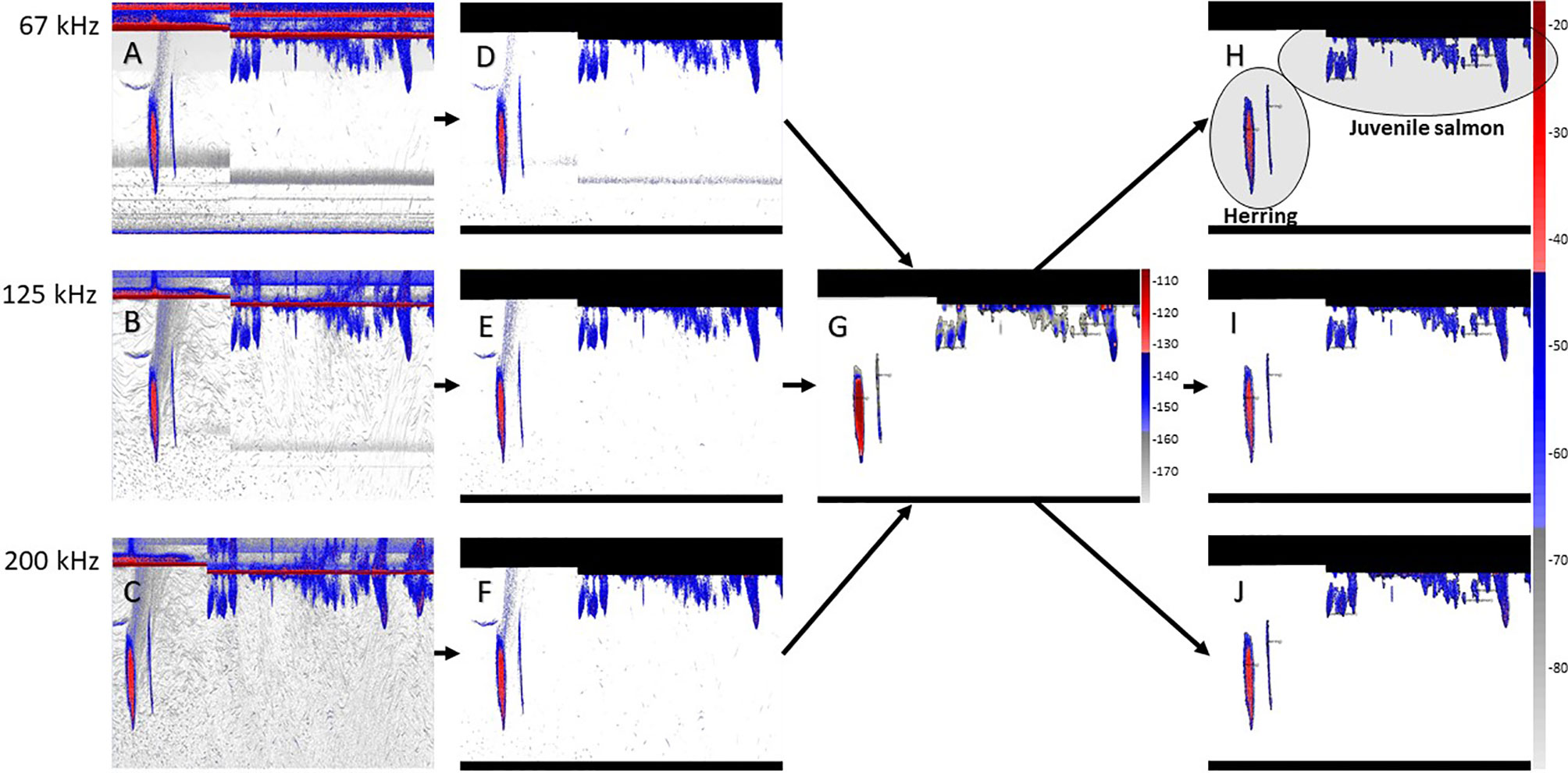
Figure 2 Steps of the acoustic data analysis: raw data at 67, 125 and 200 kHz, respectively (A–C) raw data after background noise has been removed and surface and near-field have been masked (D–F) sum of all three echograms and school detection (G) and school regions applied to echograms (H–J). The colorbar shows the volume backscattering strength (dB re 1 m). The colorbar on the right-hand side also applies to echograms (A–F), while echogram (G) shows a different scale. The vertical range represented in the echograms is approximately 50 meters. The echograms cover a period of 20 minutes on May 13 2015 (herring school), and a period of 30 minutes on May 19, 2015 (juvenile salmon schools)

A multi-frequency method developed by Fernandes (2009) was used to remove data outside of fish schools for the purpose of improving the single-frequency SHAPES algorithm (Coetzee, 2000) implemented in Echoview for school detection (Barange, 1994). This method proved efficient at removing all non-fish signals, as well as several bands of noise caused by side lobes and multiple surface reverberations present in the 67 kHz echograms (see Rousseau et al., 2018 for details). Acoustic data at 67, 125 and 200 kHz were thresholded to -70 dB to remove non-fish echoes and summed across all frequencies. The resulting combined virtual echograms were thresholded empirically to -180 dB. A 5x5 median convolution kernel was applied to remove single targets and noise spikes, followed by a 7x7 dilation convolution kernel to compensate for any loss of data within schools caused by the previous filtering steps. Finally, a mask was applied onto the raw data to all acoustic signal excluded through the previous steps.

Fish schools were detected on the masked raw data thresholded at -70 dB. An imaginary GPS linear track of 1 knot (0.51 m/s) was generated to convert the time units into virtual distance, since Echoview required GPS input to apply the school detection algorithm. A minimum horizontal threshold corresponding to 29 seconds and a minimum vertical threshold of 1 m were selected for fish school detection.

The depth of each school was determined by subtracting their mean range from the range of the acoustically detected surface. Schools were detected between sunrise and sunset hours only. At night, both juvenile salmon and herring lose their schooling behavior and tend to spread out in scattering layers, making it more difficult to distinguish the two species.Schools were classified through expert scrutiny based on the groundtruth information gathered from the on-site imaging sonar and purse seine surveys, as well as information from trawl-verified Pacific herring schools along the coast of Vancouver Island. All salmon species were included in the same class, as their echoes and behavior are likely too similar to allow for an acoustic classification.

The difference in backscatter at all three frequencies (ΔMVBS) was calculated (in the logarithmic domain) for each school and used as predictor variables in the random forest. The transducers’ beam width at half power varied from 10° at 67 kHz to 8° and 9° at 125 kHz and 200 kHz, respectively, resulting in a maximum diameter difference of approximately 2 meters at the surface. The relatively long period for school detection (29 seconds at a minimum) ensured that the school occupied the transducers’ beam footprint, and that the packing density (fish m^-3) inside the two beams was comparable.

The following 23 variables were exported from Echoview for each school: mean S_{v 67kHz} (dB), mean S_{v 125kHz} (dB), mean S_{v 200kHz} (dB), minimum S_{v 67kHz} (dB), maximum S_{v 67kHz} (dB), thickness (vertical extent) (m), perimeter (m), area (m²), skewness of S_{v 67kHz} distribution, kurtosis of S_{v 67kHz} distribution, coefficient of variation of S_v 67kHz distribution, horizontal roughness coefficient of the S_{v 67kHz} distribution (dB re 1 m² m^-3), 3D volume (m³), area backscattering coefficient at 67 kHz (ABC, m² m^-2), mean distance from transducer (m), mean depth (m), number of samples, time interval (seconds), date, time of day, ΔMVBS_67-125kHz (dB), ΔMVBS_67-200kHz (dB), and ΔMVBS_125-200kHz (dB). Unless otherwise stated, predictors derived from the acoustic data were calculated from the school’s signal at 67 kHz, because swim bladdered fish backscatter is slightly stronger at lower frequencies (Lavery et al., 2007).

Random Forest Model

Classification and regression trees are an increasingly popular statistical approach and have been used notably in ecology (De’ath and Fabricius, 2000), psychology and medical sciences (Strobl et al., 2009). This approach is particularly useful in cases where the data is complex, relationships non-linear, and the number of predictor variables is high (Breiman et al., 1984). Random forest models, in particular, are easy to implement, with very little tuning required (Hastie et al., 2009). They are not affected by correlations and interactions between variables, and do not overfit (Breiman, 2001).

A random forest is a modification of bagging, where a collection of classification trees grown on bootstrap samples of observations, cast a vote on the most popular class. During the tree growing process, each node is split using a random subset (m) of predictor variables (p). The unpruned trees and ensemble averaging work to reduce bias (the difference between the true mean and the average of the estimate) and variance (the expected deviation around its mean) (Hastie et al., 2009).The random forest analysis was implemented in the R software environment using the party package (Hothorn et al., 2006; Strobl et al., 2007; Strobl et al., 2008). The cforest function in the party package uses conditional inference, an unbiased recursive partitioning algorithm, to select predictor variables through permutation-based significance tests. Strobl et al. (2007) demonstrate that this unbiased recursive partitioning method, applied by subsampling without replacement rather than bootstrapping, results in unbiased variable selection, in contrast to the CART algorithm implemented in the randomForest package (Liaw and Wiener, 2002).The dataset was composed of 2659 acoustic regions (see Figure 2) representing 343 herring schools and 2316 juvenile salmon schools. Because such an imbalanced dataset can lead to poor prediction performance (Chen et al., 2004), we chose to down sample the dominant class, as it was shown to lead to better performance than over-sampling (Drummond and Holte, 2003). A training dataset was first created by randomly extracting 80% of the schools from each class, and then extracting a 15% subsample from the juvenile salmon class. As a result, 80% of the data corresponding to herring was used in the training dataset, in contrast to 12% for the juvenile salmon schools. The remaining 20% of data from each class was used for validation of the random forest model.The 23 variables initially selected were evaluated for collinearity to eliminate redundancy. Random forests do not require that all variables be non-correlated; however, correlated variables may make the importance order of each variable unclear (Breiman, 2001). The following statistics were conducted to verify collinearity: partial correlation (Whittaker, 1990), collinearity in a linear model (Chambers et al., 1992), and the variance inflation factor (Naimi et al., 2014). As such, the following 13 non-correlated predictors were subsequently retained for the analyses (Table 2): mean S_{v 67kHz}, mean S_{v 125kHz}, minimum S_{v 67kHz}, ΔMVBS_67-125kHz and ΔMVBS_67-200kHz, thickness, area, kurtosis, coefficient of variation, mean depth, time interval, date and time of day.Several parameters can be tuned to optimize the random forest model. In practice, values should be selected as to minimize the out-of-bag error estimate (oob error). The oob error is a means to estimate the accuracy of the model (Liaw and Wiener, 2002; Hastie et al., 2009). Its value is obtained by dividing the number of wrongful classifications by the total number of samples. The oob error becomes almost identical to a K-fold cross-validation as bootstrap samples increase (Hastie et al., 2009). For node size, Hastie et al. (2009) recommend a value of 1, the minimum size of the terminal nodes of the forest. Increasing this number causes smaller trees to be grown. The choice of the number of trees to generate (ntree) should minimize the out-of-bag error estimate (oob error); however, a larger number of trees is preferable to increase the accuracy of variable importance (Breiman, 2002). The variable importance describes the ranked importance of each variable in improving classification accuracy. For classification, the default value for the number of random subsets m to be selected at each node is √p, but it should be chosen in order to minimize the oob error. Increasing m will decrease bias but increase variance (Hastie et al., 2009). In situations where few variables are relevant in the prediction process, a very small m may result in a decrease in prediction accuracy, because many of the trees being built will not incorporate any of the relevant variables (Díaz-Uriarte and Alvarez de Andrés, 2006).Here, a m value of 2 predictors per splits was selected as it minimized the oob error. For the number of trees, the oob error was computed for ntree up to 2000. The oob error decreased rapidly until it reached a minimum around ntree = 50. It reached stability at ~ 1250 trees. To ensure the accuracy of variables importance and the stability of the model, we chose a ntree value of 1500, as it did not increase computing time significantly.Variable importance was measured using the permutation accuracy importance method. This method as well as several alternatives are discussed in Strobl et al. (2007, 2008; 2009). The permutation accuracy importance looks at the difference in accuracy before and after permuting each predictor variable to assess the importance of each variable in predicting the classification. This method allows for an unbiased measure of variable importance compared to other methods such as the Mean Decrease in Accuracy and the Gini Index, in particular in cases where missing values are present, when predictor variables vary in their scale of measurement or their number of categories, and when some of the predictor variables are correlated.We evaluated model performance with three different metrics: accuracy (K = 1 – oob), true skill statistic (TSS = Sensitivity + Specificity - 1, Allouche et al., 2006) and area under the receiver operating characteristic (ROC) curve (hereby named AUC), which represents the true positive rate (TPR, or sensitivity) plotted against the false positive rate (FPR, 1 – specificity) over a continuum of thresholds (Fielding and Bell, 1997; Kuhn and Johnson, 2013). Accuracy is the most direct way to evaluate the model; however, ROC curves and TSS are insensitive to class imbalance (Allouche et al., 2006; Kuhn and Johnson, 2013). Allouche et al. (2006) show that TSS is correlated with AUC, as they are both derived from sensitivity and specificity. Nevertheless, we present and discuss both metrics here. For the purpose of specificity and sensitivity calculations, juvenile salmon schools were selected as the primary class (positives), while herring schools were selected as the secondary class (negatives).

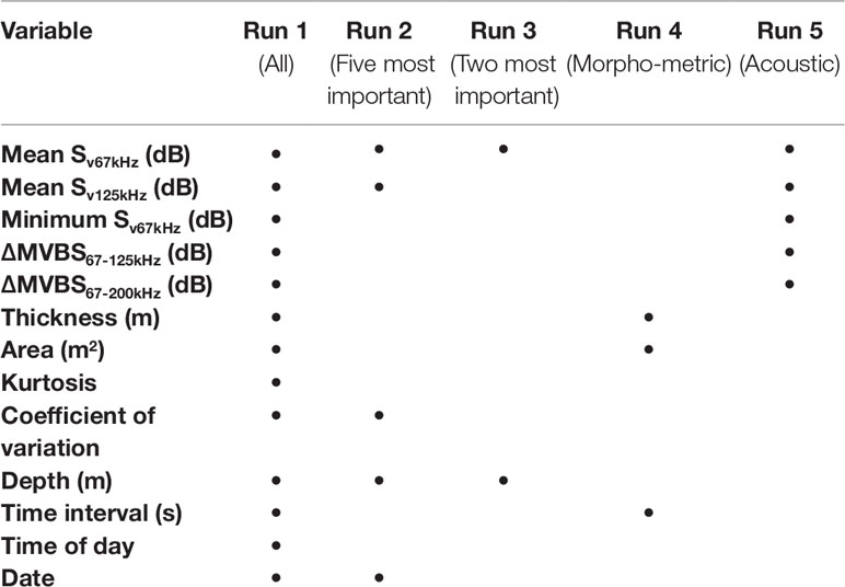
Table 2 Variables included in each random forest model.

Results

When including all non-correlated variables, the accuracy measures on the validation dataset were 98.1, 97.8 and 98.9% for K, TSS and AUC, respectively (Table 3). Table 4 shows the confusion matrix and the oob error for the training and validation datasets. Mean depth was the most important variable, followed by mean S_{v 67kHz} and date. Coefficient of variation, mean S_{v 125kHz}, ΔMVBS_67-200kHz, ΔMVBS_67-125kHz and thickness followed, but their order varied slightly depending on the random selection of the training dataset. Minimum S_{v 67kHz}, area, time interval, time of day and kurtosis were the least important predictors (Figure 3).

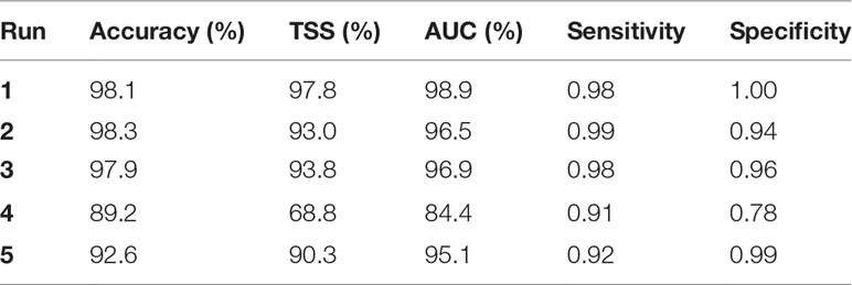
Table 3 Performance metrics of the validation dataset for each random forest model.

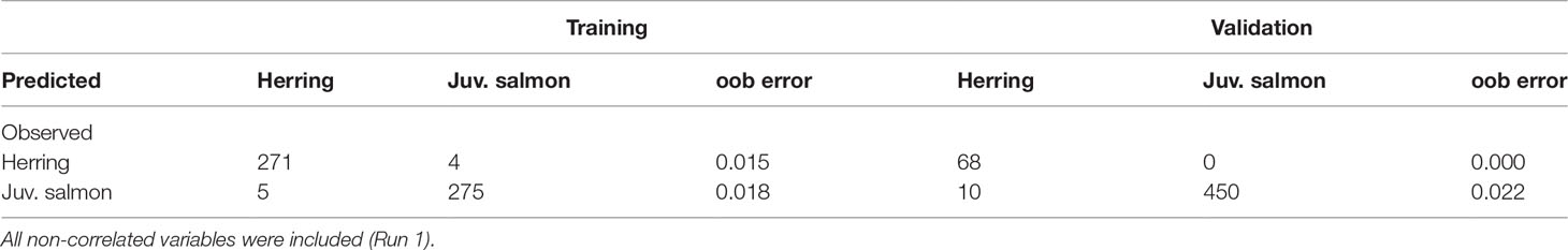
Table 4 Confusion matrix for random forest generated using training dataset of 555 and validation dataset of 528 randomly selected regions.

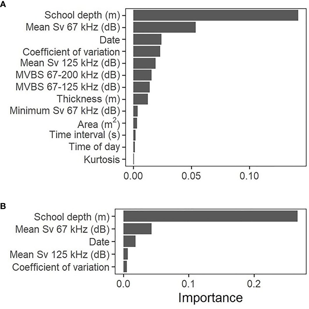
Figure 3 Importance of variables in the random forest model using all non-correlated variables (A) and 5 most important variables (B).

When conducting the random forest on the five most important variables (Table 5), K increased slightly to 98.3%, while TSS and AUC both decreased (93.0 and 96.5%, respectively). The variable importance remained unchanged, except for a swap between the mean S_{v 125kHz} and coefficient of variation variables. Kuhn and Johnson (2013) show that using non-informative predictors in random forests may lower performance. However, the decrease in the TSS and AUC values, originating from a low (0.94) specificity in the validation dataset, suggests that in this case, keeping all predictors did improve performance.

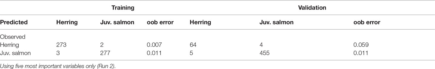
Table 5 Confusion matrix for random forest generated using training dataset of 555 and validation dataset of 528 randomly selected schools.

Using only the two most important variables, mean S_{v 67kHz} and mean depth, all metrics remained close to the previous values (97.9, 93.8 and 96.9% for K, TSS and AUC, respectively). Using only the main morphometric variables (thickness, time interval and area) decreased the performance metrics to 89.2, 68.8 and 84.4% for K, TSS and AUC, respectively. Using only the main acoustic variables (mean S_{v 67kHz}, mean S_{v 125kHz}, ΔMVBS_67-125kHz, ΔMVBS_67-200kHz and minimum S_{v 67kHz}) resulted in values of 92.6, 90.3 and 95.1% for K, TSS and AUC, respectively.TSS consistently provided the lowest performance metric, due to lower specificity values in the validation dataset. TSS decreased by 4.8 and 4% when removing all but five and two predictors, respectively. Run 5, which used only acoustic variables, presented the lowest sensitivity-to-specificity ratio, meaning that the model performed better at classifying herring than juvenile salmon in this case. AUC values were higher than TSS but lead to similar conclusions in model performance.

Discussion

Variable Importance

School depth and mean S_v67kHz were the dominant predictors to classify juvenile salmon and herring schools. Many other studies report the importance of school depth in classification accuracy (Lawson et al., 2001; Cabreira et al., 2009; D’Elia et al., 2014). Juvenile salmon were commonly found nearer the surface, whereas herring schools were most often found at mid and deep water during day time. The acoustic signal of a herring school is generally strong, as they form tight schools and swim in a synchronized fashion (Blaxter, 1985). In contrast, our DIDSON surveys showed that juvenile salmon, although exhibiting strong directional swimming following a disturbance (i.e. avoidance reaction), generally formed loose aggregations and were less polarized, resulting in a generally lower mean S_{v 67kHz} and mean S_{v 125kHz}.

During this study, a temporal mismatch was observed between juvenile salmon and herring in the area (Figure 4). Juvenile salmon migrated through the area mainly between May and July, while herring, although present throughout the summer, were found in larger numbers in August and September. This explains the importance of the date predictor. Including data from several years may help improve the transferability of the model if the date variable is included, since the timing of juvenile salmon migration and the presence of herring in the area may change from one year to the next. The inclusion of environmental data, such as temperature, may also help improve classification, since it can influence migration timing (Corten, 2001; Sykes et al., 2009).

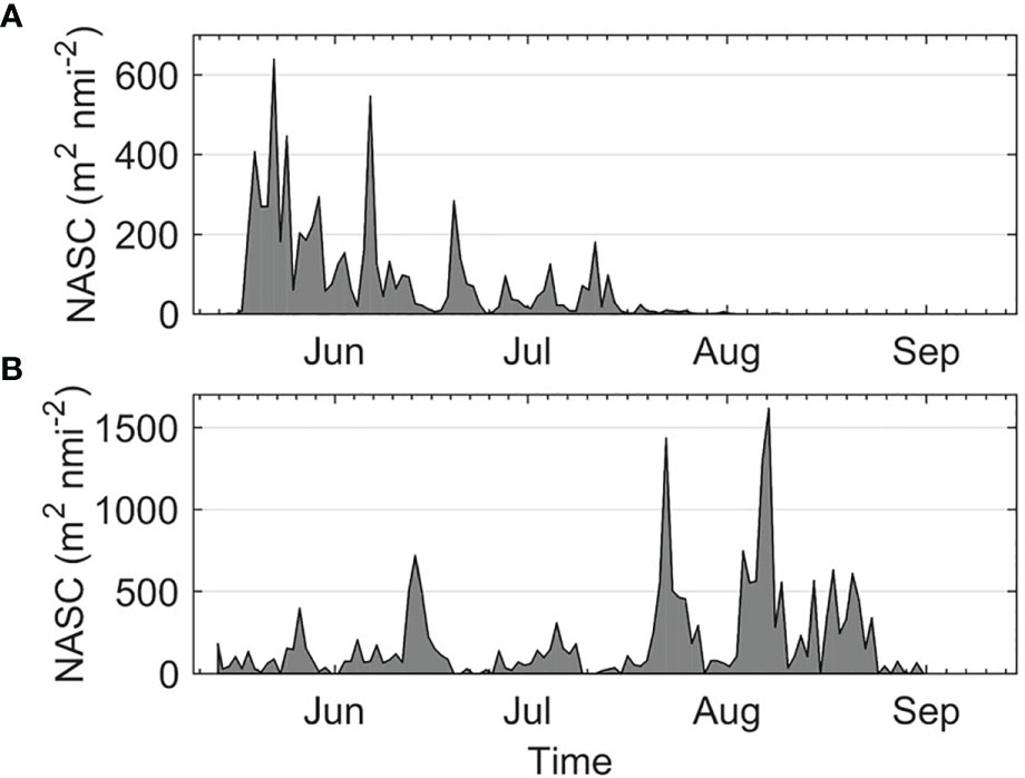
Figure 4 Nautical area backscattering coefficient (m² nmi^-2) for juvenile salmon (A) and herring (B).

The model results suggest that mean S_v is a better classifier than ΔMVBS in the case of juvenile salmon and herring schools. Mean S_{v 67kHz} and mean S_{v 125kHz} ranked second and fifth in prediction importance, respectively, while ΔMVBS_67-125kHz and ΔMVBS_67-200kHz ranked seventh and sixth, respectively. Indeed, the probability density functions of juvenile salmon and herring schools ΔMVBS show a greater overlap than that of their mean S_v (Figure 5).

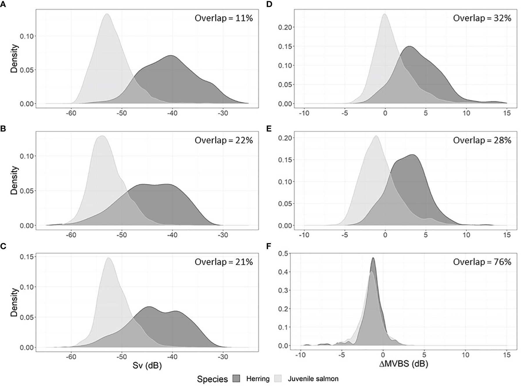
Figure 5 Probability density functions of the mean volume backscattering strength of juvenile salmon and herring schools at 67, 125 and 200 kHz (A-C), and of the difference in mean volume backscattering strength between the 67, 125 and 125 kHz frequencies for juvenile salmon and herring schools (D-F).

The importance of the coefficient of variation reflects the schooling behavior of each species. The acoustic signal of herring schools was stronger at the center, possibly reflecting a higher fish density compared to along the edges, although this could be the result of beam volume averaging. In contrast, the acoustic signature of juvenile salmon schools was generally weaker and more uniform, following our findings from the DIDSON surveys that individuals in juvenile salmon aggregations swam rather loosely and did not exhibit strongly polarized swimming, except during escaping events.Our results suggest that using all 13 non-correlated predictors selected for this study leads to the best model performance, mostly due to the higher error rates in the classification of the herring class when applying the model to the validation dataset, when variables are removed. Mean depth and mean S_v67kHz were the most important variables in the classification process, and were sufficient on their own to provide a model accuracy greater than 90% with all performance metrics.

Advantage of Random Forests Over Other Classification Methods

Echoview offers a school classification algorithm that allows the user to conduct classification using many selection criteria, including the most important variables in this study, mean S_v and range (or depth). However, the thresholds for these criteria must be selected manually by the analyst, through trial and error, which makes the selection process subjective and time-consuming. The advantage of the random forest method is that variable interaction is taken into account, and that the threshold selection does not rely on the analyst, because it is chosen within the model to minimize error.

Fallon et al. (2016) used a random forest approach to distinguish icefish, krill and mixed aggregations of weak scattering fish species and obtained an accuracy (K) of 95%. In their study, minimum S_v, mean aggregation depth (m), mean distance from the seabed (m), and geographic positional data were the most important variables in improving classification accuracy. Proud et al. (2020) also used a random forest model to classify Dagaa fish from other scatterers in Lake Victoria. Their most important variables were school length, school height and school Nautical Area Scattering Coefficient (NASC), whereas temperature, dissolved oxygen and turbidity were not important classification factors. Although environmental variables did not contribute significantly to the classification in their study, it may still be relevant to consider such variables since they are often measured in conjunction to acoustic surveys, are easily included into the random forest model, and can influence the distribution of many species of fish, including Pacific salmon and Pacific herring (Schweigert, 1995; Azumaya et al., 2007).

A brief review of the literature reveals that in recent years, the development of machine learning methods to classify active acoustic data has converged toward random forests and deep neural networks (Fallon et al., 2016; Brautaset et al., 2020; Proud et al., 2020; Sarr et al., 2020; Marques et al., 2021; Blanluet et al., 2022). In their study, Sarr et al. (2020) obtained the best and most stable performance with a random forest model when the training dataset was small, while a deep neural network gave the best performance with a large training dataset. Woodd-Walker et al. (2003) also evaluated a simple artificial neural network technique with a small training data set, but reported poor results for the least dominant class of their imbalanced dataset. Given that fisheries acoustic studies are often plagued with a lack of groundtruthing, random forests are likely the best candidate in many situations, although more studies comparing both methods would be required to draw conclusions. Using the same data source as this study, Marques et al. (2021) proposed a deep learning approach based on an instance segmentation framework to identify Pacific herring and juvenile Pacific salmon schools, using pixel-level annotations of 67 kHz echograms. While they obtained good results on unclassified schools (best performance of 92.12 mean average precision (mAP)), the performance was lower for classified schools (performance of 60.18 and 40.19 average precision (AP) for herring and juvenile salmon, respectively, using the same model configuration as for unclassified schools).

Deep neural networks have the advantage of requiring very little data pre-processing as they can draw information from the raw data (Brautaset et al., 2020), resulting in reduced analysis time and effectively removing challenges associated with bottom detection and school definition. On the other hand, random forests can incorporate a large number of variables to improve classification and provide information on the importance of each variable. This can prove advantageous not only to improve the classifier, but also to guide which variables should be monitored and sampled in the field in priority and which samples may be dropped with limited consequences on classification accuracy. It can also provide useful scientific insight into which environmental factors may be important in influencing fish population dynamics, thus contributing to the improvement of population models used in an ecosystem approach to fisheries management.

Conclusion

To our knowledge, this study is the first to attempt to classify two swim bladdered fish species using a random forest approach. We automated the school detection and classification process using Fernandes (2009) multi-frequency method and Echoview’s school detection algorithm, followed by a random forest model, and were able to differentiate between juvenile salmon and herring schools with an accuracy of 98% and higher, depending on the performance metric used. For long-term monitoring studies, consistency in the classification is as important as accuracy. Machine learning methods such as random forests not only provide this consistency by removing human bias associated with manual post-processing of the acoustic data, but they also reduce data processing time significantly. Proper data labeling is critical to reduce bias and improve accuracy of the classification model. However, a model biased by errors in the validation of the acoustic data only propagates an uncertainty that was already present with the “expert scrutiny” approach. Thus, although not ideal, a machine learning approach trained with imperfectly validated data is still preferable, because it leads to a systematic bias rather than an unpredictable uncertainty that is linked to the analyst’s choices. Over time, the algorithm’s accuracy can be iteratively improved with the addition of newly validated data to the training dataset, and this updated algorithm can easily be applied to previously analyzed data to ensure consistency.

Data Availability Statement

The raw data supporting the conclusions of this article will be made available by the authors, without undue reservation.

Ethics Statement

Lethal sampling of fish for inspection purposes, abundance estimates and other population parameters required for stock assessments are exempted from requiring an animal use protocol under the Department of Fisheries and Oceans' Pacific Region Animal Care Committee (PRACC).

Author Contributions

SR contributed to conceptualization, study design, investigation, methodology, data curation, formal analyses, programming, writing of the original draft and manuscript revision. SG contributed to conceptualization, investigation, study design, funding acquisition, project administration, resources, and manuscript revision. CN contributed to study design, investigation, funding acquisition and data curation. MT contributed to study design, funding acquisition and manuscript revision. SJ contributed to study design and funding acquisition. All authors contributed to the article and approved the submitted version.

Funding

Funding was provided by the Pacific Salmon Commission Southern Boundary Restoration and Enhancement Fund (grant number P-15-01-002). The purpose of this fund is to support activities that support salmon stocks and their habitat by developing improved information for resource management.

Conflict of Interest

The authors declare that the research was conducted in the absence of any commercial or financial relationships that could be construed as a potential conflict of interest.

Publisher’s Note

All claims expressed in this article are solely those of the authors and do not necessarily represent those of their affiliated organizations, or those of the publisher, the editors and the reviewers. Any product that may be evaluated in this article, or claim that may be made by its manufacturer, is not guaranteed or endorsed by the publisher.

Acknowledgments

We thank George Cronkite, John Morrison, Ben Snow, Chelsea Stanley, and Svein Vagle for their assistance with acoustic-related field work, as well as Nordic Queen Captain Harol Sewig and his crew for their assistance with purse seine sampling. Julia Bradshaw, Dylan Conover, Cameron Freshwater, Yeongha Jung and Lenora Turcotte assisted with fish sampling and measurements in the field. Jackie Detering analyzed the DIDSON data. This work was supported by the Pacific Salmon Commission Southern Boundary Restoration and Enhancement Fund and the Aquaculture Collaborative Research and Development Program.

References

Allouche O., Tsoar A., Kadmon R. (2006). Assessing the Accuracy of Species Distribution Models: Prevalence, Kappa and the True Skill Statistic (TSS). J. Appl. Ecol. 43, 1223–1232. doi: 10.1111/j.1365-2664.2006.01214.x
Azumaya T., Nagasawa T., Temnykh O. S., Khen G. V. (2007). Regional and Seasonal Differences in Temperature and Salinity Limitations of Pacific Salmon (Oncorhynchus Spp.). North Pac. Fish. Commun. Bull. 4, 179–187.
Barange M. (1994). Acoustic Identification, Classification and Structure of Biological Patchiness on the Edge of the Agulhas Bank and its Relation to Frontal Features. S. Afr. J. Mar. Sci. 14, 333–347. doi: 10.2989/025776194784286969
Beacham T. D., Beamish R. J., Candy J. R., Wallace C., Tucker S., Moss J. H., et al. (2014). Stock-Specific Migration Pathways of Juvenile Sockeye Salmon in British Columbia Waters and in the Gulf of Alaska. Trans. Am. Fish. Soc 143, 1386–1403. doi: 10.1080/00028487.2014.935476
Blanluet A., Gastauer S., Cattanéo F., Goulon C., Grimardias D., Guillard J. (2022). Discrimination Between Schools and Submerged Trees in Reservoirs: A Preliminary Approach Using Narrowband and Broadband Acoustics. Can. J. Fish. Aquat. Sci. 79, 738–748. doi: 10.1139/cjfas-2021-0087
Blaxter J. H. S. (1985). The Herring: A Successful Species? Can. J. Fish. Aquat. Sci. 42 (Suppl.1), 21–30. doi: 10.1139/f85-259
Boldt J. L., Gauthier S., King S. (2019). Proceedings of the National Workshop on Filling in the Forage Fish Gap. Can. Tech. Rep. Fish. Aquat. Sci. 3287, v + 82.
Boldt J., Gauthier S., Thompson M., Flostrand L., Hodes V., Nephin J. (2016). State of the Physical, Biological and Selected Fishery Resources of Pacific Canadian Marine Ecosystems in 2015. Can. Tech. Rep. Fish. Aquat. Sci. 3179, viii + 230.
Bourne C., Murphy H., Adamack A., Lewis K. (2021). Assessment of Capelin (Mallotus Villosus) in 2J3KL to 2018. DFO Can. Sci. Advis. Sec. Res. Doc. 2021/055, iv + 39.
Brautaset O., Waldeland A. U., Johnsen E., Malde K., Eikvil L., Salberg A. B., et al. (2020). Acoustic Classification in Multifrequency Echosounder Data Using Deep Convolutional Neural Networks. ICES J. Mar. Sci. 77, 1391–1400. doi: 10.1093/icesjms/fsz235
Breiman L. (2001). Random Forests Mach. Learn 45, 5–32. doi: 10.1023/A:1010933404324
Breiman L. (2002) Manual on Setting Up, Using, and Understanding Random Forests V3.1. Available at: http://oz.berkeley.edu/users/breiman/Using_random_forests_V3.1.pdf.
Breiman L., Friedman J., Olshen R. A., Stone C. J. (1984). “Classification And Regression Trees,” Chapman & Hall/CRC (Boca Raton, FL), 369 pp.
Cabreira A. G., Tripode M., Madirolas A. (2009). Artificial Neural Networks for Fish-Species Identification. ICES J. Mar. Sci. 66, 1119–1129. doi: 10.1093/icesjms/fsp009
Chamberland J.-M., Lehoux C., Émond K., Vanier C., Paquet F., Lacroix-Lepage C., et al. (2022). Atlantic Herring (Clupea Harengus) Stocks of the West Coast of Newfoundland (NAFO Division 4R) in 2019. DFO Can. Sci. Advis. Sec. Res. Doc. 2021/076, v + 115.
Chambers J. M., Freeny A., Heiberger R. M. (1992). “Chapter 5 of,” in Wadsworth & Brooks/Cole. Eds. Chambers J. M., Hastie T. J.(Pacific Grove, California).
Chen C., Liaw A., Breiman L. (2004). Using Random Forest to Learn Imbalanced Data (Berkeley: University of California).
Coetzee J. (2000). Use of a Shoal Analysis and Patch Estimation System (SHAPES) to Characterise Sardine Schools. Aquat. Living Resour. 13 (1), 1–10. doi: 10.1016/S0990-7440(00)00139-X
Corten A. (2001). Northern Distribution of North Sea Herring as a Response to High Water Temperatures and/or Low Food Abundance. Fish. Res. 50, 189–204. doi: 10.1016/S0165-7836(00)00251-4
D’Elia M., Patti B., Bonanno A., Fontana I., Giacalone G., Basilone G., et al. (2014). Analysis of Backscatter Properties and Application of Classification Procedures for the Identification of Small Pelagic Fish Species in the Central Mediterranean. Fish. Res. 149, 33–42. doi: 10.1016/j.fishres.2013.08.006
De’ath G., Fabricius K. E. (2000). Classification and Regression Trees: A Powerful Yet Simple Technique for Ecological Data Analysis. Ecology 81 (11), 3178–3192. doi: 10.1890/0012-9658(2000)081[3178:CARTAP]2.0.CO;2
De Robertis A., Higginbotton I. (2007). A Post-Processing Technique for Estimation of Signal-to-Noise Ratio and Removal of Echosounder Background Noise. ICES J. Mar. Sci. 64, 1282–1291. doi: 10.1093/icesjms/fsm112
De Robertis A., McKelvey D. R., Ressler P. H. (2010). Development and Application of an Empirical Multifrequency Method for Backscatter Classification. Can. J. Fish. Aquat. 67, 1459–1474. doi: 10.1139/F10-075
Díaz-Uriarte R., Alvarez de Andrés S. (2006). Gene Selection and Classification of Microarray Data Using Random Forest. BMC Bioinf. 79: 738–748. doi: 10.1186/1471-2105-7-3
Drummond C., Holte R. (2003). “C4.5, Class Imbalance, and Cost Sensitivity: Why Undersampling Beats Over-Sampling,” in Proceedings of the ICML-2003 Workshop: Learning from Imbalanced Data Sets II. Washington, DC, USA.
Edwards A. M., Berger A. M., Grandin C. J., Johnson K. F. (2022). Status of the Pacific Hake (Whiting) Stock in U.S. And Canadian Waters in 2022. Prepared by the Joint Technical Committee of the U.S. And Canada Pacifc Hake/Whiting AgreementNational Marine Fisheries Service and Fisheries and Oceans Canada, 238 p.
Echoview Software Pty Ltd (2015). Echoview® version 8.0. Echoview Software Pty Ltd, Hobart, Australia.
Fallon N. G., Fielding S., Fernandes P. G. (2016). Classification of Southern Ocean Krill and Icefish Echoes Using Random Forests. ICES J. Mar. Sci. 73 (8), 1998–2008. doi: 10.1093/icesjms/fsw057
Fernandes G. P. (2009). Classification Trees for Species Identification of Fish-School Echotraces. ICES J. Mar. Sci. 66, 1073–1080. doi: 10.1093/icesjms/fsp060
Fielding A. H., Bell J. F. (1997). A Review of Methods for the Assessment of Prediction Errors in Conservation Presence/Absence Models. Environ. Conserv. 24, 38–49. doi: 10.1017/S0376892997000088
Francois R. E., Garrison G. R. (1982). Sound Absorption Based on Ocean Measurements: Part I: Pure Water and Magnesium Sulfate Contributions. J. Acoust. Soc Am. 72 (3), 896–907. doi: 10.1121/1.388170
Freshwater C., Trudel M., Beacham T. D., Gauthier S., Johnson S. C., Neville C. M., et al. (2019). Individual Variation, Population-Specific Behaviours and Stochastic Processes Shape Marine Migration Phenologies. J. Anim. Ecol. 88, 67–78. doi: 10.1111/1365-2656.12852
Gauthier S., Oeffner J., O’Driscoll R. L. (2014). Species Composition and Acoustic Signatures of Mesopelagic Organisms in a Subtropical Convergence Zone, the New Zealand Chatam Rise. Mar. Ecol. Prog. Ser. 503, 23–40. doi: 10.3354/meps10731
Gauthier S., Stanley C., Nephin J. (2016). State of the Physical, Biological and Selected Fishery Resources of Pacific Canadian Marine Ecosystems in 2015. Can. Tech. Rep. Fish. Aquat. Sci. 3179, viii + 230. Distribution and abundance of Pacific Hake (Merluccius productus). In Chandler, P.C., King, S.A., and Perry, R.I. (Eds.) (2016).
Haegele C. W., Hay D. E., Schweigert J. F., Armstrong R. W., Hrabok C., Thompson M., et al. (2005). Juvenile Herring Surveys in Johnstone Strait and Georgia Straits – 1996 to 2003. Can. Data Rep. Fish. Aquat. Sci. 1171, xi + 243.
Hastie T., Tibshirani R., Friedman J. (2009). The Elements Statistical Learning (London: Springer), 763 pp.
Hothorn T., Buehlmann P., Dudoit S., Molinaro A., van der Laan M. (2006). Survival Ensembles. Biostatistics 7 (3), 355—373. doi: 10.1093/biostatistics/kxj011
Johannesson K. A., Mitson R. B. (1983). “Fisheries Acoustics: A Practical Manual for Aquatic Biomass Estimation,” in FAO Fish. Tech. Paper 240 (Rome: FAO), 249 pp.
Kaartvedt S., Rostad A., Klevjer T. A., Staby A. (2009). Use of Bottom-Mounted Echo Sounders in Exploring Behavior of Mesopelagic Fishes. Mar. Ecol. Prog. Ser. 395, 109–118. doi: 10.3354/meps08174
Lavery A. C., Wiebe P. H., Stanton T. K., Lawson G. L., Benfield M. C., Copley N. (2007). Determining Dominant Scatterers of Sound in Mixed Zooplankton Populations. J. Acoust. Soc Am. 122 (6), 3304–3326. doi: 10.1121/1.2793613
Lawson G. L., Barange M., Fréon P. (2001). Species Identification of Pelagic Fish Schools on the South African Continental Shelf Using Acoustic Descriptors and Ancillary Information. ICES J. Mar. Sci. 58, 275–287. doi: 10.1006/jmsc.2000.1009
Mackenzie K. V. (1981). Nine-Term Equation for the Sound Speed in the Oceans. J. Acoust. Soc Am. 70 (3), 807–812. doi: 10.1121/1.386920
Marques T. P., Côté M., Rezvanifar A., Albu A., Ersahin K., Mudge T., et al. (2021). Instance Segmentation-Based Identification of Pelagic Species in Acoustic Backscatter Data. 2021 IEEE/CVF Conference on Computer Vision and Pattern Recognition Workshops (CVPRW). IEEE, 4373–4382. doi: 10.1109/CVPRW53098.2021.00494
McClathie S., Thorne R. E., Grimes P., Hanchet S. (2000). Ground Truth and Target Identification for Fisheries Acoustics. Fish. Res. 47 (2-3), 173–191. doi: 10.1016/S0165-7836(00)00168-5
Mckinnell S., Curchitser E., Groot K., Kaeriyama M., Trudel M. (2014). Oceanic and Atmospheric Extremes Motivate a New Hypothesis for Variable Marine Survival of Fraser River Sockeye Salmon. Fish. Oceanogr. 23 (4), 322–341. doi: 10.1111/fog.12063
Naimi B., Hamm N. A. S., Groen T. A., Skidmore A. K., Toxopeus A. G. (2014). Where is Positional Uncertainty a Problem for Species Distribution Modelling? Ecography 37 (2), 191–203. doi: 10.1111/j.1600-0587.2013.00205.x
Neville C. M., Johnson S. C., Beacham T. D., Gauthier S., Whitehouse T., Tadey J., et al. (2016). Initial Estimates From an Integrated Study Examining the Residence Period and Migration Timing of Juvenile Sockeye Salmon From the Fraser River Through Coastal Waters of British Columbia. NPAFC Bull. 6, 45–60. doi: 10.23849/npafcb6/45.60
Parker-Stetter S. L., Rudstam L. G., Sullivan P. J., Warner D. M. (2009). Standard Operating Procedures for Fisheries Acoustic Surveys in the Great Lakes. Great Lakes Fish. Commun. Spec. Pub. 09-01. 168p.
Proud R., Mangeni-Sande R., Kayanda R. J., Cox M. J., Nyamweya C., Ongore C., et al. (2020). Automated Classification of Schools of the Silver Cyprinid Rastrineobola Argentea in Lake Victoria Acoustic Survey Data Using Random Forests. ICES J. Mar. Sci. 77 (4), 1379–1390. doi: 10.1093/icesjms/fsaa052
R Core Team (2019). R: A Language and Environment for Statistical Computing (Vienna, Austria: R Foundation for Statistical Computing). Available at: http://www.R-project.org/.
Rousseau S., Gauthier S., Johnson S. C., Neville C. M., Trudel M. (2018). Juvenile Salmon Acoustic Monitoring in the Discovery Islands, British Columbia. Can. Tech. Rep. Fish. Aquat. Sci. 3277, viii + 32.
RStudio Team (2018). RStudio: Integrated Development for R (Boston, MA: RStudio Inc.). Available at: http://www.rstudio.com/.
Sarr J. M. A., Brochier T., Brehmer P., Perrot Y., Bah A., Sarré A., et al. (2020). Complex Data Labeling With Deep Learning Methods: Lessons From Fisheries Acoustics. ISA Trans. 109, 113–125. doi: 10.1016/j.isatra.2020.09.018
Sato M., Dower J. F., Kunze E., Dewey R. (2013). Second-Order Seasonal Variability in Diel Vertical Migration Timing of Euphausiids in a Coastal Inlet. Mar. Ecol. Prog. Ser. 480, 39–56. doi: 10.3354/meps10215
Sato M., Horne K. J., Parker-Stetter S. L., Keister J. E. (2015). Acoustic Classification of Coexisting Taxa in a Coastal Ecosystem. Fish. Res. 172, 130–136. doi: 10.1016/j.fishres.2015.06.019
Schweigert J. F. (1995). 121. Environmental Effects on Long-Term Population Dynamics and Recruitment to Pacific Herring (Clupea pallasii) Populations in Southern British Columbia: Climate Change and Northern Fish Populations. Can. Spec. Publ. Fish. Aquat. Sci./Publ. Spec. Can. Sci. Halieut. Aquat., Ottawa ON, 121, 569-583.
Simmonds J., MacLennan D. (2005). Fisheries Acoustics: Theory and Practice. Second Edition (London: Blackwell Publishing).
Simmonds E. J., Williamson N. J., Gerlotto F., Aglen A. (1991). Survey Design and Data-Analysis Procedures: A Comprehensive Review of Good Practice Vol. 54 (Copenhagen: ICES). Int. Counc. Explor. Sea CMB.
Strobl C., Boulesteix A. L., Kneib T., Augustin T., Zeilis A. (2008). Conditional Variable Importance for Random Forests. BMC Bioinf. 9 (307), 1–11. doi: 10.1186/1471-2105-9-307
Strobl C., Boulesteix A. L., Zeileis A., Hothorn T. (2007). Bias in Random Forest Variable Importance Measures: Illustrations, Sources and a Solution. BMC Bioinf. 8 (25), 1–25. doi: 10.1186/1471-2105-8-25
Strobl C., Malley J., Tutz G. (2009). An Introduction to Recursive Partitioning: Rationale, Application, and Characteristics of Classification and Regression Trees, Bagging, and Random Forests. Psychol. Methods 14 (4), 323–348. doi: 10.1037/a0016973
Sykes G. E., Johnson C. J., Shrimpton J. M. (2009). Temperature and Flow Effects on Migration Timing of Chinook Salmon Smolts. Trans. Am. Fish. Soc 138, 1252–1265. doi: 10.1577/T08-180.1
Thompson M., Fort C., Boldt J. (2016). Strait of Georgia Juvenile Herring Survey, September 2014. Can. Manuscr. Rep. Fish. Aquat. Sci. 3087, v + 45 p.
Thomson R. E., Allen S. E. (2000). Time Series Acoustic Observations of Macrozooplankton Diel Migration and Associated Pelagic Fish Abundance. Can. J. Fish. Aquat. Sci. 57, 1919–1931. doi: 10.1139/f00-142
Trumble R. J., Humphreys R. D. (1985). Management of Pacific Herring (Clupea Harengus Pallasii) in the Eastern Pacific Ocean. Can. J. Fish. Aquat. Sci. 42 (Suppl. 1), 230–244. doi: 10.1139/f85-277
Tucker S., Trudel M., Welch D. W., Candy J. R., Morris J. F. T., Thiess M. E., et al. (2009). Seasonal Stock-Specific Migrations of Juvenile Sockeye Salmon Along the West Coast of North America: Implications for Growth. Trans. Am. Fish. Soc 138, 1458–1480. doi: 10.1577/T08-211.1
Watkins J. L., Brierley A. S. (2002). Verification of the Acoustic Techniques Used to Identify Antarctic Krill. ICES J. Mar. Sci. 59, 1326–1336. doi: 10.1006/jmsc.2002.1309
Keywords: random forest, machine learning, acoustic classification, salmon, herring
Citation: Rousseau S, Gauthier S, Neville C, Johnson S and Trudel M (2022) Acoustic Classification of Juvenile Pacific Salmon (Oncorhynchus spp) and Pacific Herring (Clupea pallasii) Schools Using Random Forests. Front. Mar. Sci. 9:857645. doi: 10.3389/fmars.2022.857645
Received: 18 January 2022; Accepted: 07 June 2022;
Published: 11 July 2022.
Edited by:
Doran M. Mason, NOAA-Great Lakes Environmental Research Laboratory, United StatesReviewed by:
Chris Taylor, National Centers for Coastal Ocean Science (NOAA), United StatesMatthew Baker, North Pacific Research Board, United States
Copyright © 2022 Rousseau, Gauthier, Neville, Johnson and Trudel. This is an open-access article distributed under the terms of the Creative Commons Attribution License (CC BY). The use, distribution or reproduction in other forums is permitted, provided the original author(s) and the copyright owner(s) are credited and that the original publication in this journal is cited, in accordance with accepted academic practice. No use, distribution or reproduction is permitted which does not comply with these terms.
*Correspondence: Shani Rousseau, shani.rousseau@dfo-mpo.gc.ca