Air-Sea Trace Gas Fluxes: Direct and Indirect Measurements

1 Introduction

The exchange of gases between the atmosphere and ocean is an important process in global budgets of many gases with significant implications in climate, biogeochemical cycles, oceanic ecosystems, and pollution. Because of its importance to global carbon budgets, biology, and climate, carbon dioxide (CO₂) tends to dominate our interest in the subject but many gases including oxygen (O₂), carbon monoxide (CO), dimethylsulfide (DMS), ozone (O₃), and sulfur dioxide (SO₂) to name a few, are also relevant - see Johnson (2010) for a list of 79 gases. The exchange of non-reactive gases are usually expressed as vertical fluxes which are principally driven by wind speed and the sea-air concentration difference of the gas. Gas fluxes may be measured directly from ships with bow-mounted eddy correlation systems or estimated from mean concentrations using so-called bulk flux relationships (Fairall et al., 2000; Wanninkhof et al., 2009). Arrays of in situ measurements are not practical for global or regional budget closure, so some combination of satellite, reanalysis, and data assimilation synthesis is needed (Cronin et al., 2019; Shutler et al., 2020). These approaches rely on the bulk relationships. Thus, the principal application of direct measurements [including deliberate dual tracer techniques, Ho et al. (2011)] is in determining the appropriate bulk scaling variables and coefficients. It turns out this is a complex issue that involves similarity theory, chemistry, laboratory studies, process models such as direct numerical and large eddy simulations (DNS and LES), and a variety of experimental approaches in the field (see Garbe et al., 2014, for an overview).

The mass flux of some scalar variable, x, can be directly estimated from measurements of turbulent correlations in the near-surface atmosphere with the direct covariance (a.k.a. eddy correlation) technique:

Here ρ_ad is the density of dry air, r_x the mixing ratio of x (mass of x per dry mass of air), w^′ and x^′ are turbulent fluctuations of vertical velocity and dry air mole fraction of x, respectively. More often though, the air-sea flux is computed using the bulk method:

where X is the mean concentration of x and the subscripts s and z refer to the value at the air-ocean interface and height z, respectively. S is the mean wind speed, C_x is the transfer coefficient for the mass flux of x, $c_x^{1/2}$ is the scalar transfer component specific to x and $u_{\ast }=\sqrt{C_d}*U_{10}$ is the friction velocity where C_d is the drag coefficient and $U_{10}=\sqrt{U^2+V^2}$ is the vector average wind speed for mean components U and V at reference height z = 10 m. Note mean wind speed is distinct from the mean vector wind components and is defined as $S^2=\overline{{(U+u^{\prime })}^2+{(V+v^{\prime })}^2}$, where the capitals and primes denote of the mean and turbulent fluctuations of the horizontal wind components. Differences between the mean wind speed, and vector-averaged winds are associated with gustiness (Fairall et al., 1996; Fairall et al., 2003).

The essence of bulk parametrizations is captured in specification of the transfer coefficient, C_x, which is obtained directly by measuring $\overline{w^{\prime }{x}^{\prime }}$, S_z, X_s, and X_z and applying (2). Note C_x will depend on z and buoyancy forcing as defined in Monin-Obukhov similarity theory (MOST – see e.g., Fairall et al. (1996)). Bulk algorithms have a long and successful history in meteorology; in this paper we will focus principally on the COARE family of flux codes (Fairall et al., 2011) where COAREG defines codes for gas transfer. There are certainly other products to choose from for gas transfer purposes, e.g., FluxEngine (Goddijn-Murphy et al., 2016; Shutler et al., 2016) or FuGas (Vieira et al., 2020).

While (2) is commonly used to estimate fluxes of sensible heat and moisture, the gas transfer community more often uses a formulation based on a transfer velocity, k_x,

where α_x is the dimensionless solubility of the gas x in seawater, k_x the transfer velocity for the gas X, X_w and X_a the mean concentrations of x at some depth in water and some height in air, and we use ΔX to denote the sea-air difference in X taking solubility into account. Note that, compared to (2), expression (3) has the additional complexity of solubility. Superficially, k_x is equivalent to $C_x{S}_z=c_x^{1/2}{u}_{\ast }$ in (2). Because C_x for heat and moisture is approximately constant with the friction velocity or wind speed, we might infer that k_x is roughly proportional to wind speed. Would that it was so simple. To illustrate the variability in transfer with the properties of trace gases, Fairall et al. (2011) recast (3) as

with CP being interpreted as characterizing the chemical variability and u_∗ΔX characterizing the physical forcing. Figure 1 in Fairall et al. (2011) shows CP varying by 4 orders of magnitude with small values (2 × 10^-6) for the highly insoluble gas neon, increasing with solubility to about 0.03 for α_x = 100 (e.g., ethanol) and then leveling off with increasing solubility. This leveling off for highly soluble gases is well understood to be the limit imposed by transfer in the atmosphere – i.e., similar to water vapor, which is unconstrained by transfer resistance on the ocean side, ${\text{CP}}_v=c_v^{1/2}\approx 0.035$. Both CO₂ (solubility on the order of 0.5) and DMS (solubility on the order of 15) are intermediate to these extremes.

Early wind tunnel measurements (Liss and Merlivat, 1986) and analysis of ¹⁴C in the ocean (Wanninkhof, 1992) found the transfer velocity of CO₂ (i.e., k_co2) to be non-linear in wind speed. Woolf (1993) argued that the stronger wind speed dependence of CO₂ was due to enhancement by bubbles generated by breaking waves. Because the enhancement was solubility dependent, Woolf predicted that more soluble gases would have a more linear wind speed dependence – a prediction that has been borne out by observations of DMS transfer velocity (e.g., Blomquist et al., 2006).

Ocean surface waves are an essential component in air-sea fluxes. The fluxes of momentum and kinetic energy from the atmosphere to the ocean are driven by a direct input to the ocean currents via viscous stress and input to waves via the pressure-wave slope correlation known as form drag. Viscous stress dominates the exchange at low wind speeds. As the winds increase, the dominant mechanism for exchange transfers to the form drag imposed primarily by wind waves with some modulation due to longer waves and swell. The action of the form drag grows waves which transfer their momentum and energy to ocean currents and turbulence initially through micro-breaking (Edson et al., 2013). The transition is complete once the waves become fully rough; a condition often associated with the onset of visible wave breaking around 7 m s^-1. At this point, bubble-mediated processes begin to gain importance (Woolf, 1993) and breaking of longer waves plays an increasingly important role in momentum and, particularly, energy exchange (Melville, 1996).

The simplicity of bulk flux relations (2) and (3) is somewhat misleading because complexity may be hidden in the transfer coefficients. The simplest forms contain little complexity, with power law dependence on wind speed at some reference height, typically 10m.

where the coefficient c_1x depends on the gas and U in m s^-1 (k_x in cm hr^-1). For CO₂ c_1x is on the order of 0.25 (Wanninkhof, 2014). However, there is debate about the power law with up to 3^rd-order polynomials in wind speed being used (Wanninkhof et al., 2009). The temperature dependence of k_x is usually captured through a temperature-dependent Schmidt number Sc_x = v/D_x, where D_x is the oceanic molecular diffusivity and 660 is the reference value of Sc_co2 at 20°C (although the 1/2 exponent may not hold in all conditions).

Since the bulk gas and water concentrations are measured well away from the interface, mixing processes in both media must be considered. This has led to the development of physically-based parameterizations that attempt to capture the relevant processes in a unified mathematical structure (e.g. Liss and Slater, 1974; Fairall et al., 2011; Goddijn-Murphy et al., 2016). If this is successful, it is not necessary to measure c_1x for each gas of interest. This is the approach for the COAREG gas flux parameterizations where both atmospheric and oceanic interfacial forcing are framed within surface-layer turbulent scaling theory. In the ocean, turbo-molecular mixing and bubble mediated transfer are treated as parallel processes.

While wave processes are important in almost all aspects of air-sea interactions, it is interesting that many very successful parameterizations do not explicitly include wave properties. This is because wave properties are highly correlated with wind speed. Thus, simple representations in the drag coefficient, C_d, or k_x are done with wind speed alone. Ironically, decades of experimental and theoretical effort (see Brumer et al., 2017a) have yet to yield wave-based parameterizations for C_d, or k_x that give significantly better RMS fits to direct observations over the open ocean. This is partly due to the large sampling noise of the observations and partly the noisy and uncertain nature of characterizations of the wave field. However, that is not the complete story because wind-only parameterizations essentially characterize transfer for a mean wave climatology associated with that wind speed. We expect that when the waves depart significantly from that mean, then air-sea fluxes may be affected. For example, in a coastal region offshore winds may yield quite different fluxes compared to onshore winds at the same wind speed, as has been observed for sea spray (Yang et al., 2019). Regardless of our ability to explicitly include wave variables in a parameterization, separating near-surface turbulent and bubble-mediated processes in physically-based treatments of gas transfer is useful.

In this paper we will further discuss air-sea fluxes – principally gas transfer and its forcing mechanisms – in the context of the COARE algorithms. We will not attempt a detailed attack on all issues (e.g., discussion in Johnson et al., 2011; Woolf et al., 2019), but focus on specific topics where significant progress has been made through observations, theory, or numerical modeling. The principal scaling variables for k_x are solubility, Schmidt number, friction velocity, and whitecap fraction. The last two variables may be estimated with wind-only formulae or with formulae that add some wave information. We begin with a discussion of theoretical background, then sketch the formulation of COARE [taking from detail provided in Fairall et al. (2011)]. We will briefly describe direct observations and focus on three recent field programs. We will discuss wave-based parameterizations and the difficulty of determining them with observations alone. Because of their more than one order of magnitude solubility differences, simultaneous DMS and CO₂ observations can be analyzed to separate the turbo-molecular and bubble-mediated components. To do this, we will also have to deal with chemical enhancement of CO₂ flux (Wanninkhof, 1992; Luhar et al., 2018; Jørgensen et al., 2020). The turbo-molecular transfer is found to be quite linear with the tangential component of the stress. The bubble component is approximately linear with either whitecap fraction or air-entrainment rate of breaking waves but there is still some uncertainty in characterizing those quantities which will be discussed.

2 Theoretical Background

In this section we describe a simple 1-dimensional theoretical framework for describing the flux-profile relationships for trace gas transport between the atmosphere and ocean. The approach has its roots in observations from wind tunnels and flat Kansas plains, so application over the ocean requires a certain skepticism. It is known that wind speed does not strictly obey the conventional log-layer behavior within the wavy boundary layer. Furthermore, distortions by wave motions on the ocean side occur on scales that are greater than the normal ‘10% of the mixed layer depth’ usually ascribed to the surface layer where ‘law of the wall’ scaling is appropriate. Our justification for using this approach for gas transfer applications is based on the small scale of the molecular sublayer and the transition to the turbulent sublayer – this occurs at mm scales where local dominant wave-induced slopes are negligible. This theoretical approach allows us to conceptualize the balance of the processes and to create a scaling structure that can be tuned to observations with only a few universal parameters.

2.1 Fluxes, Solubility, Similarity and Turbo-Molecular Transport

In the absence of significant in situ sources or sinks, the vertical flux of some scalar variable, x, in either fluid can be defined as the sum of molecular and turbulent diffusivities

In the case where z is height or depth, the flux is positive directed away from the interface. Near the surface the turbulent flux can be represented in terms of the local gradient and a turbulent eddy diffusivity, K(z), so that

We can integrate (8) from the surface to some reference height (depth), z_r, to obtain the total change of X between the surface (subscript s) and z_r,

If we define an air-side transfer velocity of x, k_xa, as acting between the surface and some reference height in the atmosphere, z_ra, then

Thus, (9) and (10) imply

Similarly, we can define a turbo-molecular flux on the water side

While temperature is continuous across the interface, gas concentrations are not so we must account for the discontinuity by defining the solubility, α_x as

If we assume the atmospheric flux is continuous with the oceanic flux (applicable to a gas not undergoing rapid chemical reactions), then we can derive (4) where

We use Monin-Obukhov Similarity (MOS) to describe the turbulent diffusivity (Fairall et al., 2000, hereafter F00): MOS defines surface turbulent flux scaling parameters u_* and x_* in terms of turbulent conditions sufficiently far from the interface that fluxes of momentum or of a scalar x (i.e. trace gases) are completely carried by turbulent covariance

The profile of a dynamical variable can be described via a dimensionally consistent combination of the scaling parameters, z, and a dimensionless function of z/L, where L is the MOS buoyancy length scale. This leads to a simple specification of turbulent diffusivity

where ɸ is an empirical function that characterizes the enhancement of diffusion in convective conditions or suppression in stratified conditions and κ is the von Karman constant, κ ≈ 0.4. Stability effects may be substantial but for dealing with near-surface and interfacial aspects of gas transfer, we can assume ɸ = 1.

F00 discuss solutions to (9) and (11) using an approximation for K(z) that accounts for the suppression of turbulence near the interface which occurs in the sublayer

Where λ is a coefficient on the order of 10. This is done by expressing K(z) as

The form of (18) produces a smooth transition from molecular-dominated diffusion to turbulent diffusion and has the effect of extending the depth of the molecular layer. The analytical solution to (9) produces a near-surface linear profile (molecular sublayer) that transitions to a logarithmic profile (turbulent sublayer)

where a = D_x δ_u, b =D_x, c = κu_*w, $d={[4D_x{\delta }_u\kappa u_{*w}-D_x^2]}^{1/2}$ G = a + bz + cz².

In principle, this solution applies to vertical transfer of dissolved gas within the ocean in the absence of chemical reactions. The analytical profile in the turbulent layer can be approximated

where 5δ_u is the maximum extent of the molecular sublayer (Zülicke, 2005) and ΔX_m characterizes the total change in X over that layer. Using λ =10, the analytical solution gives

The logarithmic form is an idealization because of the distortions of the wave motions. At heights well above the significant wave height, atmospheric logarithmic profiles are observed over the ocean (e.g. Edson et al., 2004). In the ocean, wave induced displacements are a significant fraction of the mixed layer depth and an idealized log-layer may not exist (Zheng et al., 2021). However, we still expect the idealized solution to reasonably describe the main aspects of the profile at cm scales.

2.2 The Wavy Boundary Layer - Viscous Stress Versus Wave Stress

Waves add another complication because of their role in the momentum transfer and the friction velocity. The fluxes of momentum and kinetic energy from the atmosphere to the ocean are, except in light winds, dominated by input to waves via the pressure-wave slope correlation – the so called form drag. The action of the wind grows waves which, when they break, transfer their momentum and energy to ocean currents and turbulence. The wind is also subject to a viscous drag which directly drives surface currents and near-surface turbulence. Far from the interface, (but still within the surface layer of the marine boundary layer), the momentum flux from the atmosphere (surface stress) can be expressed as the covariance of atmospheric turbulent velocity fluctuations similar to (1)

where u^′ represents fluctuations of wind speed in the in the mean wind direction (for simplicity, we ignore the crosswind stress component). Near the air-sea interface (even within the influence of surface wave disturbances) the momentum flux is the sum of viscous, turbulent, and wave-pressure components τ_v, τ_t, τ_g. Thus, while the total stress may be assumed to be approximately constant in height, the turbulent τ_t, component is not constant in the wave boundary layer (Ortiz-Suslow et al., 2021). At the interface, turbulence is negligible, and so the momentum flux delivered to the ocean is the sum of viscous (subscript v) and gravity wave drag (subscript g)

Viscous (tangential) drag is the product of the air kinematic viscosity with the wind gradient at the surface (subscript s), while the gravity wave drag is the correlation of ‘ pressure fluctuations, p’, and the wave slope’ rho is the symbol for density, p the symbol for pressure (ƞ is the vertical displacement of the surface by waves) and x_u is the horizontal coordinate in the mean wind direction. Soloviev (2007) and Fairall et al. (2011) argue that, at scales less than 1 m near the interface, u_*av should scale with the turbulent diffusion because the wave-pressure correlation has reduced the turbulent momentum flux. This has been discussed in more detail by Cifuentes-Lorenzen et al. (2018) who suggest the wave stress component decays exponentially with a height scale of about 1 m. The portioning suggested by (23) can be written

Cifuentes-Lorenzen et al. (2018) use the parameter α_g which is the fraction of wave stress to total stress so that

Fairall et al. (2011)) give an estimate of the ratio of viscous to total stress as

and provide a simple formulation [see Figure B1 in Fairall et al. (2011)]. Figure 1 shows estimates of α_g as a function of 10-m wind speed and wave age, c_p/U₁₀ where c_p is the phase speed of the waves with frequency corresponding to the peak of the wave energy spectrum. α_g is small at low winds and increases with wind speed; viscous and wave components of stress are comparable at wind speeds on the order of 12 m s^-1 (see Figure 1). Friction velocity on the ocean side is computed assuming the atmospheric viscous stress drives the oceanic viscous stress:

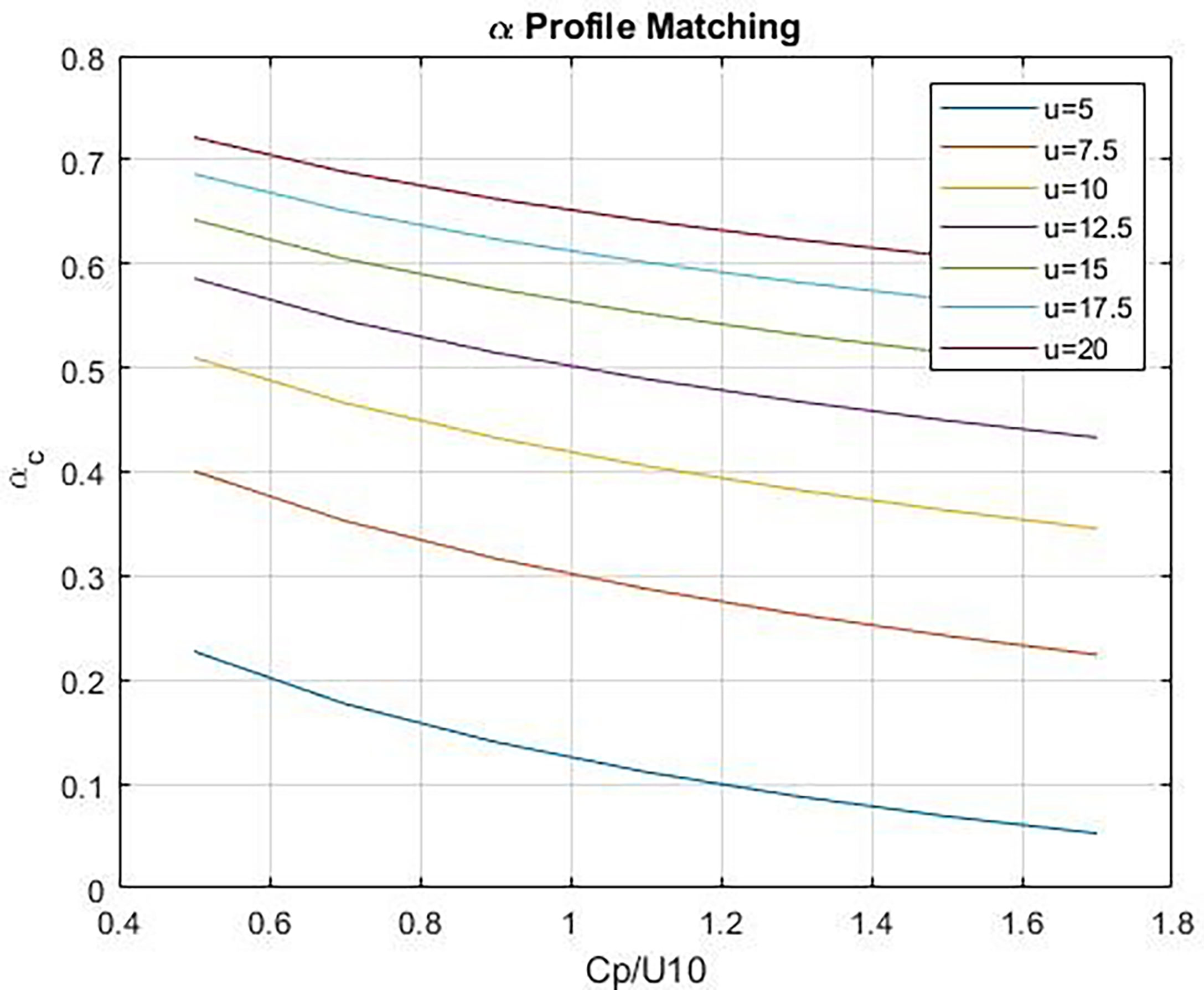
Figure 1 Wave stress fraction, α_g, vs wave age, Cp/U₁₀, at different values of u = U₁₀. The lower curves correspond to lower wind speeds.

2.3 Atmospheric and Ocean Side Turbulent-Molecular Diffusion and Bubbles

On the atmospheric side of the interface, the behavior of k_xa is well-constrained by direct covariance flux measurements of water vapor [see Figure 4 in Fairall et al. (2000)] and other trace gases of high solubility/reactivity (Yang et al., 2014; Yang et al., 2016; Porter et al., 2020). While (11) implies a sensitivity of k_xa to molecular diffusivity, it turns out that the variation of atmospheric diffusivity amongst trace gases of interest is not significant (Rowe et al., 2011). Direct flux measurements of soluble trace gases to date (Yang et al., 2016; Porter et al., 2020) have shown some departures from water vapor or heat, but the measurement techniques are probably not sufficiently accurate to reject a simple water vapor analogy representation. The importance of air-side transfer declines as solubility declines. For DMS (solubility on the order of 15) k_xa contributes about 5% to (14) while for CO₂ (solubility on the order of 0.5) it contributes about 0.2%. For solubility greater than 100, k_xa dominates (14) and k_x/u_*a≈k_xa/u_*a≈0.03.

On the ocean side of the interface the total transfer is assumed to be the sum of turbo-molecular, k_v, and bubble-mediated, k_b, processes:

The turbo-molecular part can be computed via (11) and (18) with the molecular sublayer part given by (21). The much smaller molecular diffusion coefficients in the ocean ( Sc_x on the order of 1000 compared to 1 in the atmosphere) imply that most of the change in trace gas concentration on the ocean side occurs in the molecular transport sublayer. Figure 2 contrasts the oceanic profiles for temperature ( Sc_t = 5.9) and CO₂ ( Sc_w = 660) at a water temperature of 20°C. The analytical solution is shown by the solid line and the log-layer portion by the dashed line. In this normalized form the log-layer slopes are the same but the offset caused by the molecular sublayer portion is relatively much larger for CO₂ – implying the computation of the flux for CO₂ is much less sensitive to specification of the depth of the ocean side concentration measurement.

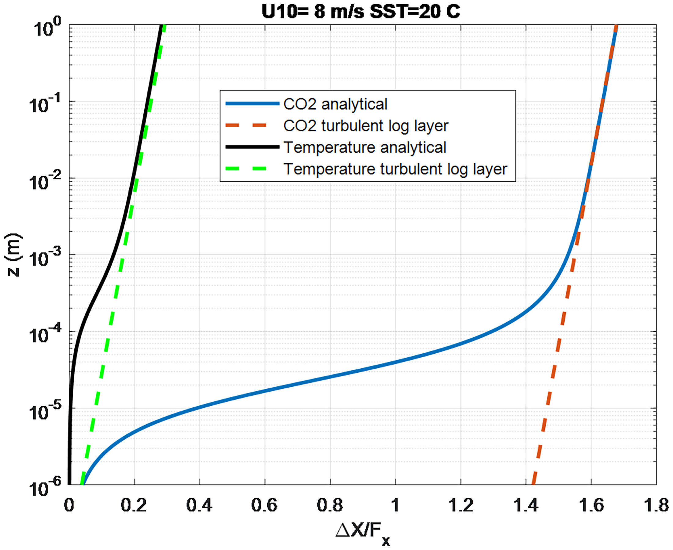
Figure 2 Normalized profiles of ocean temperature and CO₂ concentration computed from the analytical solution (solid lines) K(z) = κzu_*/(1+δ_u/z). The dashed lines are using (21) to represent the turbulent log-layer part of the profile.

Bubble-mediated transfer is associated with air entrained by breaking waves. Wave breaking that entrains air rarely occurs in lighter wind regimes with a crude threshold of U₁₀ ≈ 5-8 m s^-1. Gas transfer enhancement by bubbles has been studied in laboratory experiments (Woolf, 1993; Rhee et al., 2007; Krall et al., 2019) and with numerical models (Woolf and Thorpe, 1991; Liang et al., 2013; Deike et al., 2017). The laboratory studies quoted here conflict somewhat on the importance of bubbles. The numerical model approach is based on injecting into the ocean a numerical plume of bubbles with a spectrum of sizes. Gas transfer from the bubbles is computed for each bubble size as the plume rises and is vertically transported; total transfer is computed by integrating over the size spectrum. Turbulent mixing of the bubble plume may be neglected or can be very sophisticated (e.g., Liang et al. (2013) use a Large Eddy Simulation model). The variety of assumptions (injection depth, rise rate, bubble spectrum, bubble transfer rates, clean vs. dirty bubble, plume density, etc) lead to a variety of outcomes. Laboratory (Callaghan, 2013; Callaghan et al., 2016; Callaghan, 2018) and numerical modeling (Deike et al., 2016; Deike and Melville, 2018) have also advanced understanding of the connection between wave breaking and dissipation, air entrainment, bubble populations, and whitecap coverage.

An example of a parameterization developed for bubble transfer can be found in Woolf (1993),

where B is an empirical constant tuned to observations, V₀ = 2450 cm hr^-1 is the air volume entrainment flux per unit whitecap fraction, f_wh is the whitecap fraction, e = 14, and n =1.2. This form is chosen so that the transfer velocity obeys the expected limits for low solubility (bubble mediated flux depends on the diffusion, but not on solubility) and high solubility (bubble mediated flux scales inversely with solubility). There is some debate about the scaling of the forcing in (29): should it be whitecap fraction, actively breaking fraction, air entrainment velocity (V), or dissipation of wave breaking energy? The Woolf form assumes the scaling is V = V₀ f_wh with whitecap fraction scaling as $U_{10}^{3.41}$ based on a fit to whitecap observations by Monahan (1971). Recent observations (Brumer et al., 2017b; Anguelova and Bettenhausen, 2019) have shown the Monahan formulation overestimates the wind-speed dependence which leads to overly large gas transfer estimates in high winds. Gas transfer versions of the COARE bulk transfer model, COAREG (Fairall et al., 2011), use (29) but Liang et al. (2013); Goddijn-Murphy et al. (2016), and Deike et al. (2017) offer viable alternatives to (29).

2.4 Chemical Enhancement

The COAREG models treat various gases with the assumption that they are conservatively transported. However, transfer of CO₂ is complicated by carbonate chemical reactions on the water side – a phenomenon referred to as chemical enhancement. Hoover and Berkshire (1969) (hereafrter HB69) express the chemical enhancement of CO₂, CE, as

where, adapting the notation of Wanninkhof and Knox (1996), TT and Q depend on CO₂–carbonate reaction rate constants and diffusivity (D_co2), and δ = D_co2/k is diffusion layer thickness. Temperature dependence is explicit in TT and Q. Wind speed dependence is implied in δ but no explicit functional form is given.

Wanninkhof (1992) (hereafter W92) considered this effect in the analysis of passive tracers to derive a formula for the enhanced transfer velocity for CO₂ k_en660. He uses a temperature-dependent but wind speed independent form for CE given by a polynomial fit, p(T), to CE(T) at a constant k of 1 cm hr^-1.

W92’s formula gives p(T) = 3 cm hr^-1 in the tropics and 2 cm hr^-1 for conditions relevant to the HiWinGS experiment (see Section 3.2). Wanninkhof and Knox (1996) define CE = k_en/k and examine the HB69 model with observations from several alkaline lakes and also estimate CE for the equatorial Pacific Ocean. Note, this implies that as k_en/k approaches 1.0 with increasing winds, CE becomes small.

More recently, Fairall et al. (2007), hereafter F07, investigated air-sea transfer of ozone by considering the 1-dimensional conservation equation with a simple chemical reaction

where flux is positive downward, X is the mean mass concentration and a_r = C_xyY is the reactivity coefficient for the reaction of constituent X and constituent Y with a reaction rate constant of C_xy. F07 assumed ozone was completely destroyed in seawater and that the reactions are with unspecified oceanic chemicals in significantly large concentration such that the reaction is pseudo first-order in X and a_r is equivalent to a rate constant (s^-1).

Here, we adapt this approach to CO₂. Following McGillis and Wanninkhof (2006), we assume the ocean mixed layer CO₂ concentration, X_e, is in near equilibrium with carbonate chemistry. We assume that X_e is the result of a balance with total carbonate and alkalinity so that in the absence of significant temperature gradients it is essentially independent of depth. This is a more complex case than for ozone, but we again make the simplifying assumption that the reaction is pseudo first order in X_e and reactivity can be represented by a simple reactivity coefficient a_r (s^-1) or time constant τ_r = 1/a_r (s). The time constant is unknown but can be estimated from measurements. Thus, for a reactive gas in equilibrium like CO₂, (32) can be written

The turbulent flux is represented in terms of turbulent diffusivity coefficient, K(z), so that

where X^′=X−X_e. Following F07, we can use (34) to define a general flux variable, F_x, as

The gradient term expresses the sum of molecular and turbulent diffusion and the second term the gain or loss of X via chemical reaction. In steady state as expressed by (35), F_x is independent of depth and equal to the flux at the interface, F_x(0) = F_xs. For non-reactive gases, we can use (35) with a_r = 0 to characterize the transport through the water

Using the analytical solution (19) for the non-reactive case, k_xw represents the transfer velocity of x on the water side to some reference depth, z, on the order of 1 m. For a_r > 0 an analytical solution corresponding to (34) with (18) does not exist. Jørgensen et al. (2020) found solutions for (34) without the near-surface turbulence suppression. Another approach was developed by Luhar et al. (2018) who solved this problem by assuming that (18) could be approximated by setting the turbulent eddy diffusion coefficient to zero within some scale δ_m of the surface (see Figure 3) and K(z) = κzu_*w for z greater than δ_m. Thus within a scalar molecular layer a stagnant (non-turbulent) film is assumed. If K(z) is set to 0 for z < δ_m, the solutions of (34) with K(z) = 0. are exponentials. So the complete profile is given by

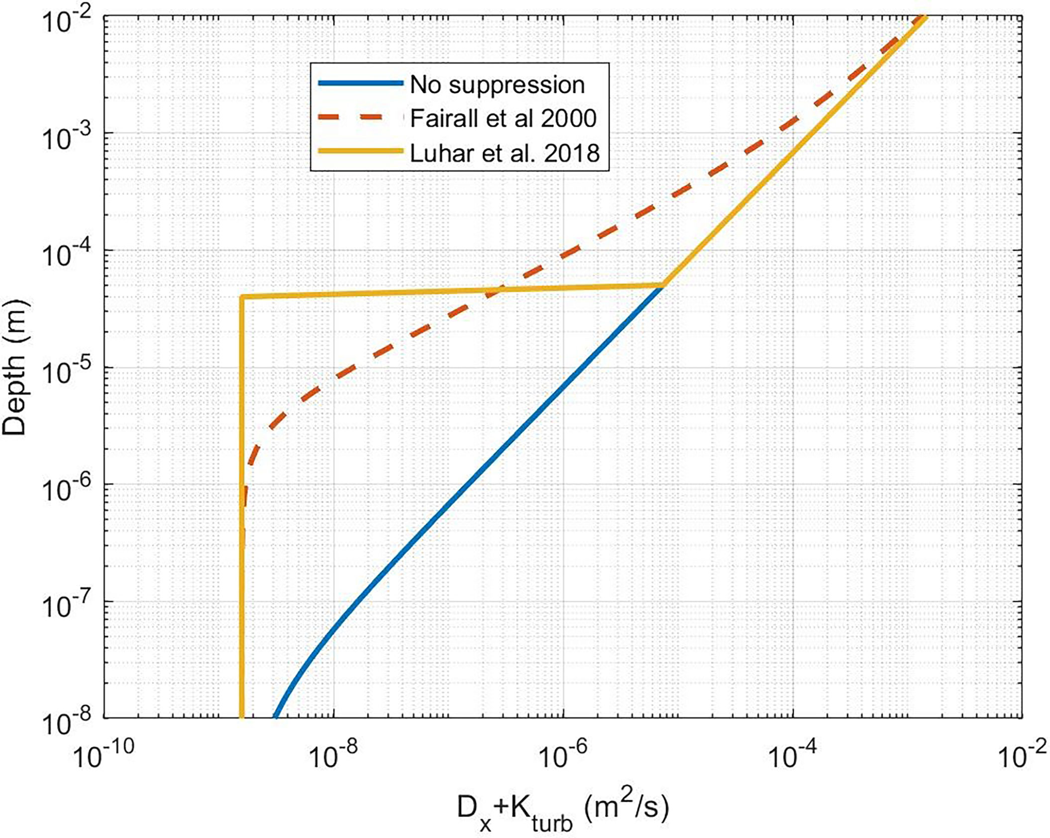
Figure 3 Near-surface profile of the sum of molecular and turbulent diffusivities. The blue line is for K(z) without near-surface dissipative suppression (Eq. (18) with δ_u = 0 ). The dashed line is (41). The yellow line is the Luhar et al. (2018) approximation using (41).

$\text{X}=\{\begin{array}{ll}{\text{A}}_1\text{exp }(\sqrt{\frac{a_r}{D_x}})+B_1\text{exp }(-\sqrt{\frac{a_r}{D_x}}),\hfill & \text{z}<={\delta }_m\hfill \\ {\text{B}}_2{K}_0\left(\xi \right),\hfill & \text{z}>{\delta }_m\hfill \end{array}$ (37a, 37b)

where A₁, B₁, B₂ are constants and K₀ is a modified Bessel function of order 0. Luhar et al. (2018) give an analytical expression for transfer velocity over some depth where chemical reactions become negligible

where K_n are modified Bessel functions of order n, ψ = [1+κ u_*w δ_m/D_x]^1/2, λ_m = δ_m(a_r/D_x)^1/2, and ξ_δ is computed from

where z = δ_m corresponds to the depth where the turbulent transport starts. Luhar et al. (2018) examined temperature dependent specifications for reactivity, a_r, and several candidates for δ_m. Their final selections captured the modest temperature and weak wind speed dependencies of observed ozone deposition velocity, but because ozone has very high reactivity they did not clearly delineate a value for δ_m.

In order to choose the optimum value for δ_m, we integrate (36) with the specified 2-layer K(z) profile with a_r = 0 and select δ_m to match the asymptotic form of the non-reactive analytical solution (21). This leads to

In our view, this is a rigorous choice because it guarantees the same transfer velocity in the absence of chemical reactions.

We can use the 2-layer model to evaluate CE for CO₂. However, a more rigorous approach is a brute-force numerical solution to (34) with (18). One advantage of this approach is we can check and/or tune the 2-layer analytical model, which can give us an analytical function for CE in terms of the forcing and a_r. The numerical solutions are computed using MATLAB^® differential equation solvers. With a_r=0, the numerical solutions agreed with the non-reactive analytical solution (F00). Results for selected values of τ_r are shown in Figure 4 where we compute the enhancement ratio via

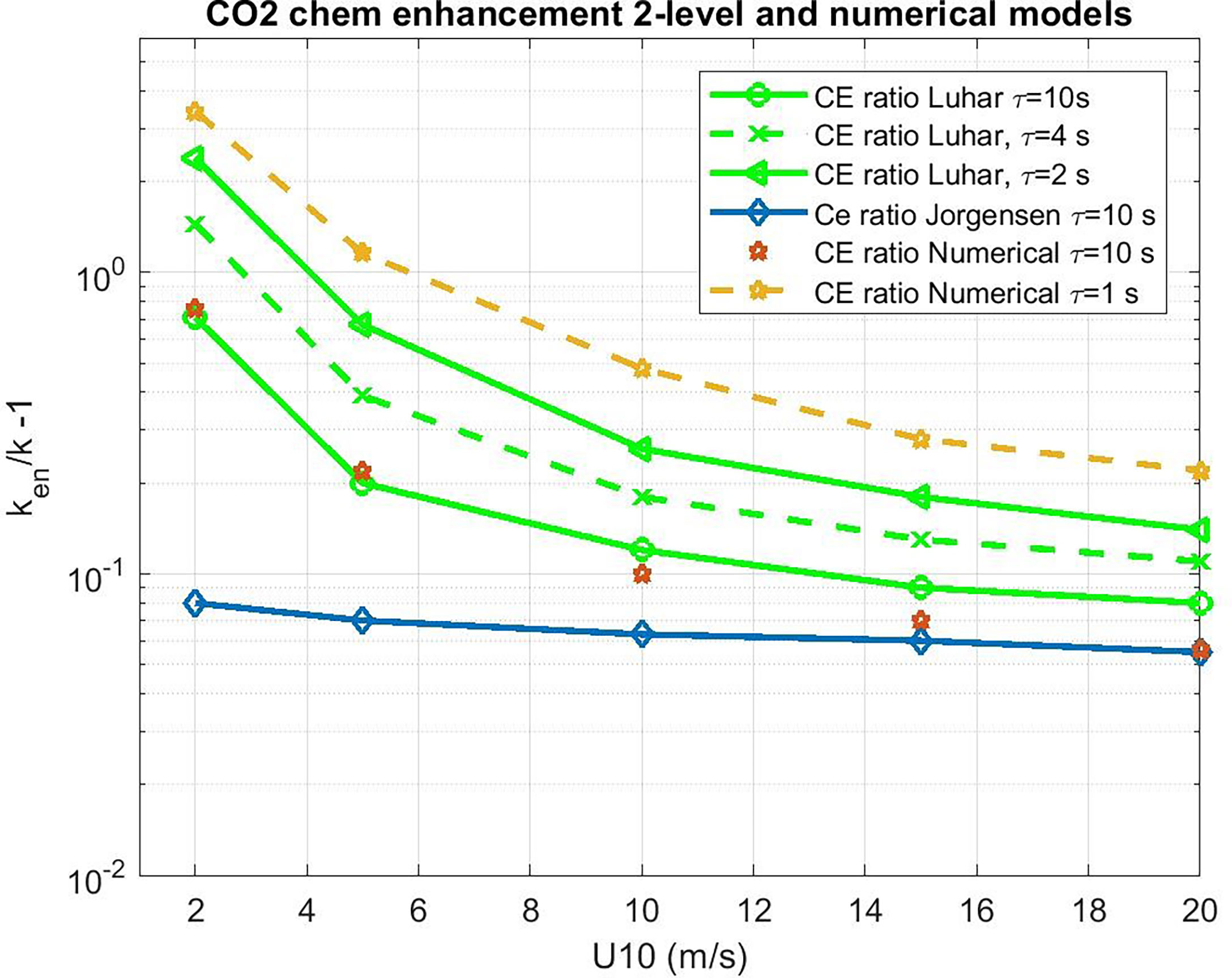
Figure 4 Water side transfer velocity (normalized to Sc = 660) ratio of chemical enhanced to background value as a function of 10-m wind speed. Estimates of chemical enhancement (CE) via (42) for CO₂ are shown with star symbols using a numerical integration of (34) and (19) and the analytical model (38) as green lines for different values of the CO₂ carbonate reaction time constant, τ_r. The results of the Jørgensen et al. (2020) are shown as diamonds.

The use of the ratio reduces the sensitivity to the calibration of k = k(a_r = 0) . We then compute CE as

which is shown in Figure 5, where the COAREG 3.1 transfer velocity for gas x, k_c31x, is the estimate for transfer without CE. The Luhar et al. (2018) analytical approximation is a good match with the numerical solution with our choice for δ_m. This solution also works well for ozone. These calculations suggest CE of 3-5 cm hr^-1 for CO₂ corresponding to a time constant, τ_r, on the order of 3 s.

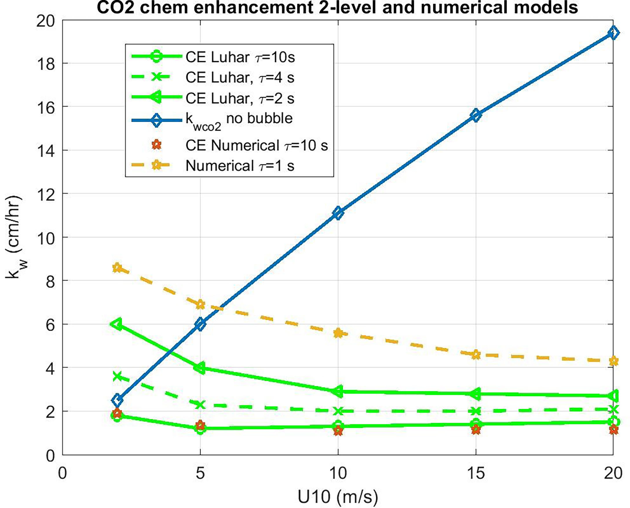
Figure 5 Water side transfer velocity (normalized to Sc = 660) as a function of 10-m wind speed. The basic COAREG non-bubble relationship for neutral conditions is shown in the blue diamonds. Estimates of chemical enhancement (CE) for CO₂ are shown using a numerical model (stars) an and an analytical model (green lines) for different values of the CO₂ carbonate reaction time constant, τ_r.

3 Direct Observations

3.1 Advances in DMS and CO₂ Flux Measurement

In this paper, we tune the latest revision of the model (COAREG 3.6) to direct gas exchange observations made with the eddy covariance (EC) method. The application of the EC method for measuring gas fluxes at sea requires high temporal resolution measurements of 1) vertical wind velocity, and 2) gas mixing ratio. The advent of the motion-correction method in late 1990s (Edson et al., 1998) enabled the derivation of the ambient vertical wind velocity from a moving platform. This method is subsequently refined by Miller et al. (2010); Landwehr et al. (2015), and Blomquist et al. (2017). Comparisons of momentum and heat fluxes between a buoy and a nearby fixed tower demonstrate that the bias due to the motion correction is within 6% (Flügge et al., 2016). For CO₂, we utilize fluxes measured using a closed-path instrument with a dryer. Deemed the best practice by Landwehr et al. (2014) and Blomquist et al. (2014), this approach avoids the water vapor cross-sensitivity in the CO₂ measurement that likely confounded earlier flux measurements, especially using an open-path infrared analyzer [e.g., Edson et al. (2011)]. In particular, cavity ringdown analyzers (e.g., Picarro G2311-f) and closed-path infrared analyzers (e.g. Licor7200) are both well suited for measurements of air-sea CO₂ flux. Recent works by Dong et al. (2021) demonstrate that the random uncertainty in hourly CO₂ flux is typically 30-50% (mostly a function of the flux magnitude), with sensor noise from both Picarro G2311-f and Licor7200 only contributing a minor fraction of the total flux uncertainty. Air-sea DMS flux measurement is made with a chemical ionization mass spectrometer operating at near atmospheric pressure. Hourly random uncertainty in DMS flux is on the order of 20-30% (Blomquist et al., 2010), thanks to the high signal-to-noise ratio in the DMS flux measurement.

3.2 Recent Field Programs

The last decade has seen over a dozen field programs dedicated to EC gas flux measurements, with at least eight cruises and several near shore deployments. Long term EC measurements have been undertaken at two coastal sites. Östergarnsholm station is located in the Baltic Sea (57°27’N, 18°59’E) and has been providing CO₂ fluxes since 1995 (Rutgersson et al., 2020). Penlee Point Atmospheric Observatory (PPAO) was established in 2014 by the Plymouth Marine Laboratory in the Plymouth Sound on the south-west coast of the United Kingdom (50°19.08’N, 4°11.35’W). It provides CO₂, CH₄ fluxes (https://www.westernchannelobservatory.org.uk/penlee,Yang et al. (2016)). A list of all recently collected and analysed EC field measurements is given in Table 1 along with references to relevant publications.

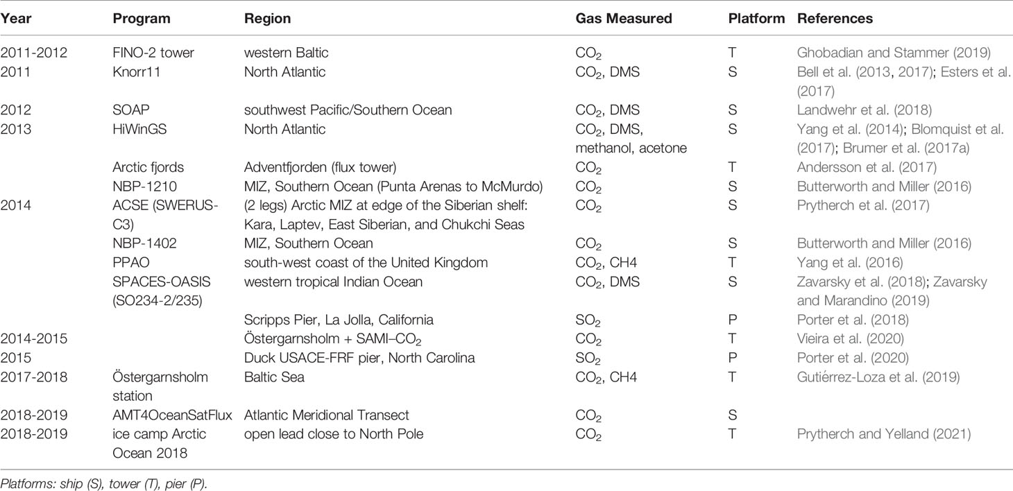
Table 1 Recent field campaigns.

In this paper we focus on results from three recent campaigns (Knorr11 in 2011, SOAP in 2012, HiWinGS in 2013), where simultaneous air-sea exchange measurements of CO₂ and DMS are available. Some published direct measurements of DMS k₆₆₀ have shown unexpected decreases at higher wind speeds: GasEx08 (Blomquist et al., 2017), Knorr11 (Bell et al., 2013; Bell et al., 2017), and Sonne-234/235 (Zavarsky and Marandino, 2019). This was discussed in depth by Zavarsky and Marandino (2019) and explained in terms of flow separation using a wave reference Reynolds number, Re_tr. The argument is that flow separation (which occurs when Re_tr < 6.5E6) suppresses the direct viscous transfer component and this affects DMS relatively more than CO₂ because the much larger bubble transfer for CO₂ masks the decrease. The basic idea has some logic, although Zavarsky et al. (2018) Figure 13 shows no dramatic decrease in DMS k₆₆₀ for HiWinGS despite a large fraction of suppressed conditions for U10 > 12 m s^-1. In our own analysis of HiWinGS data, using their Re_tr criterion, we find no significant difference in k₆₆₀ for DMS in suppressed vs. non-suppressed conditions, but CO₂ k₆₆₀ is reduced by about 10 cm h^-1 during ‘suppressed’ conditions. It seems the sudden decrease in k₆₆₀ DMS in strong winds observed in some field programs remains puzzling.

4 Analysis of Observations in a COARE Context

4.1 Turbo-Molecular and Bubble-Mediated Drivers

The last public release of the COAREG algorithm, version 3.1 (Fairall et al., 2011), does not include CE and gives a simple form for the transfer velocity (14) which captures the net transfer across water (w) and atmospheric (a) surface layers We can separate the oceanic and atmospheric components as follows

From measurements of k, we can compute the oceanside value, k_w, which is made up of a turbulent-molecular term, k_v, and a bubble-mediated term, k_b. For HiWinGS the term multiplying k in (43) is an average of 1.054 for DMS and 1.008 for CO₂. Following Appendix A of Fairall et al. (2011), we can convert k_w to k₆₆₀ and write (43) as

Here the first term on the right hand side represents tangential (interfacial) transfer, while the second term indicates bubble-mediated gas exchange (see Eq. 29). A and B are parameters tuned to fit the observations and the temperature- and gas-dependent factors are

with n = 1.2. In (44) we have neglected buoyancy effects on the first term, which become more important at wind speeds less than 5 m s^-1. Note that in COAREG, k_v is scaled by viscous, rather than total, friction velocity.

We can now consider the form of (44) for both CO₂ (subscript c) and DMS (subscript d) with the temperature dependent factors in k_b, V₀ and α(20) combined into the single factors b_c and b_d

If k values are expressed in cm hr^-1, then the factor b_c ≅ 830, while b_d = 130 + 2.6T where T is in °C. Thus, the ratio between bubble-mediated gas exchange of DMS and that of CO₂, r_dc = b_d/b_c, in (46b) varies from 0.16 to 0.22 with an average of 0.18 for HiWinGS. The relationships in (46) can be applied to observations of k for CO₂ and DMS to estimate the constants A and B:

Note (47) is approximate because it uses mean values for T-dependent factors, but if (47) is applied to k_w values computed with the COAREG algorithm, then for a 10-m wind speed adjusted to neutral conditions, U_10n > 5 m s^-1, the values for A and B assumed in the algorithm will be recovered within 10%. Also, note that the value of A depends on the form of the friction velocity factor and B depends on choice of whitecap formulation. If the model and the measurements are consistent, then the values of A and Bshould be independent of wind speed.

Figure 6 shows values of A and B extracted from HiWinGS observations averaged in wind speed bins. To reduce the effects of flux sampling uncertainty, values of CO₂ transfer velocities were only used if the absolute value of sea-air partial pressure difference Δp_co2 exceeded 20 μatm. Two retrievals have been done: 1) with bin averages of measured k_w660 and 2) using power-law fits of k_w660 to wind speed in the form

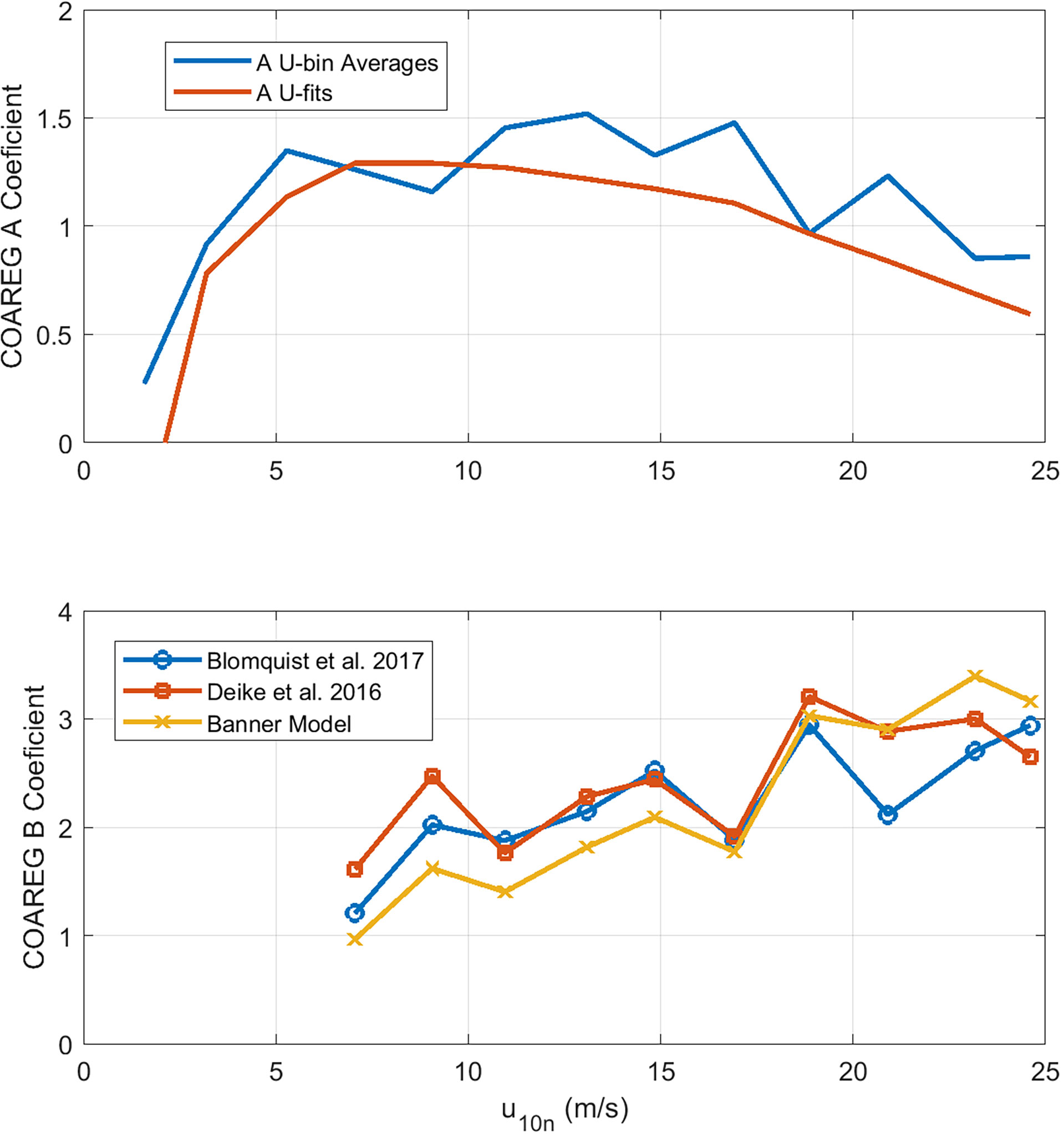
Figure 6 Retrieved values of COAREG constants, A (upper panel) and B (lower panel), as a function of wind speed. For A, retrievals are based on mean values of observed k_w660 averaged in wind speed bins plus values of k_w660 computed from wind-speed power law fits. For B , only the wind speed bin results are shown. There are curves for three possible choices of f_wh. Data for U_10n < 6 are not shown because no whitecaps were observed.

We have used c₀ = 6.0, c₁ = 0.41, and m = 1.9 for CO₂; c₀ = 0.6, c1 = 1.09, and m = 1.2 for DMS. To compute B (47b), both retrievals used bin-averaged estimates of whitecap fraction computed from Brumer et al. (2017b)

Averaging both retrieval methods yields A = 1.25 and B = 2.3, using (49) for whitecap fraction. We have also used bin-averaged values of observed f_wh; that yields noisier results but does not significantly change the final estimates of A and B.

In Figure 7 we show a comparison of transfer velocities averaged in wind speed bins from the three calculation methods: linear+bubble (46); wind speed power law (48); and a new version of COAREG using these values of A and B and the Brumer et al. (2017b) whitecap formulation – we are referring to this as COAREG36. A summary of the mean and RMS statistics is given in Table 2. Since the power law is fit directly to the mean observations, it gives the best overall fit.

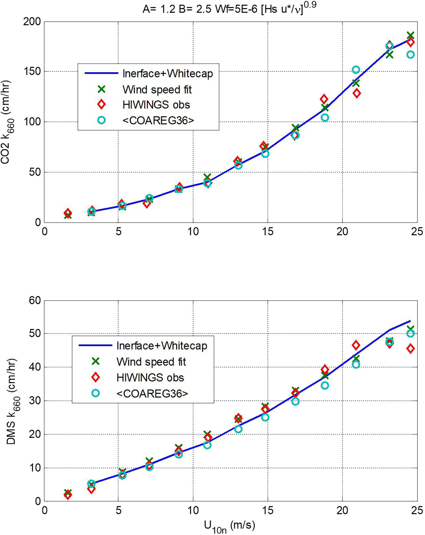
Figure 7 Values of k_w660 (upper panel, CO₂; lower panel, DMS) averaged in wind speed bins vs. 10-m neutral wind speed. The red diamonds are mean observed values, the x’s are from the wind speed power-law fits (48), the blue line is from (46) using A = 1.2 and B = 2.5, and the circles are means of values computed using COAREG36.

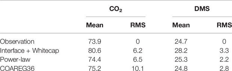
Table 2 Summary of mean k₆₆₀ (cm hr^-1) and RMS difference from mean HiWinGS measurements.

So far our specification of total gas transfer velocity (46) requires the turbo-molecular term to scale with u_*v and the bubble-mediated term to scale with f_wh. It is insightful to reevaluate the turbo-molecular and bubble terms separately without specifying the nature of the forcing. So we recast (47) without the u_*v and f_wh factors but assume the forcing will have some wind speed dependence:

The results are shown in Figure 8 as a function of 10-m wind speed. Also shown on the graphs are the COAREG forms for the forcing: f(U) = u_*v and g(U) = f_wh . We can see that the turbo-molecular term is nearly linear with the viscous stress and showing a hint of saturation at higher winds speeds. This could imply that our parametrization of viscous stress is too high and our parameterization underestimates the importance of the wave stress component at high winds speeds. The bubble-mediated term has a much stronger wind speed dependence and is well represented by the whitecap parameterization.

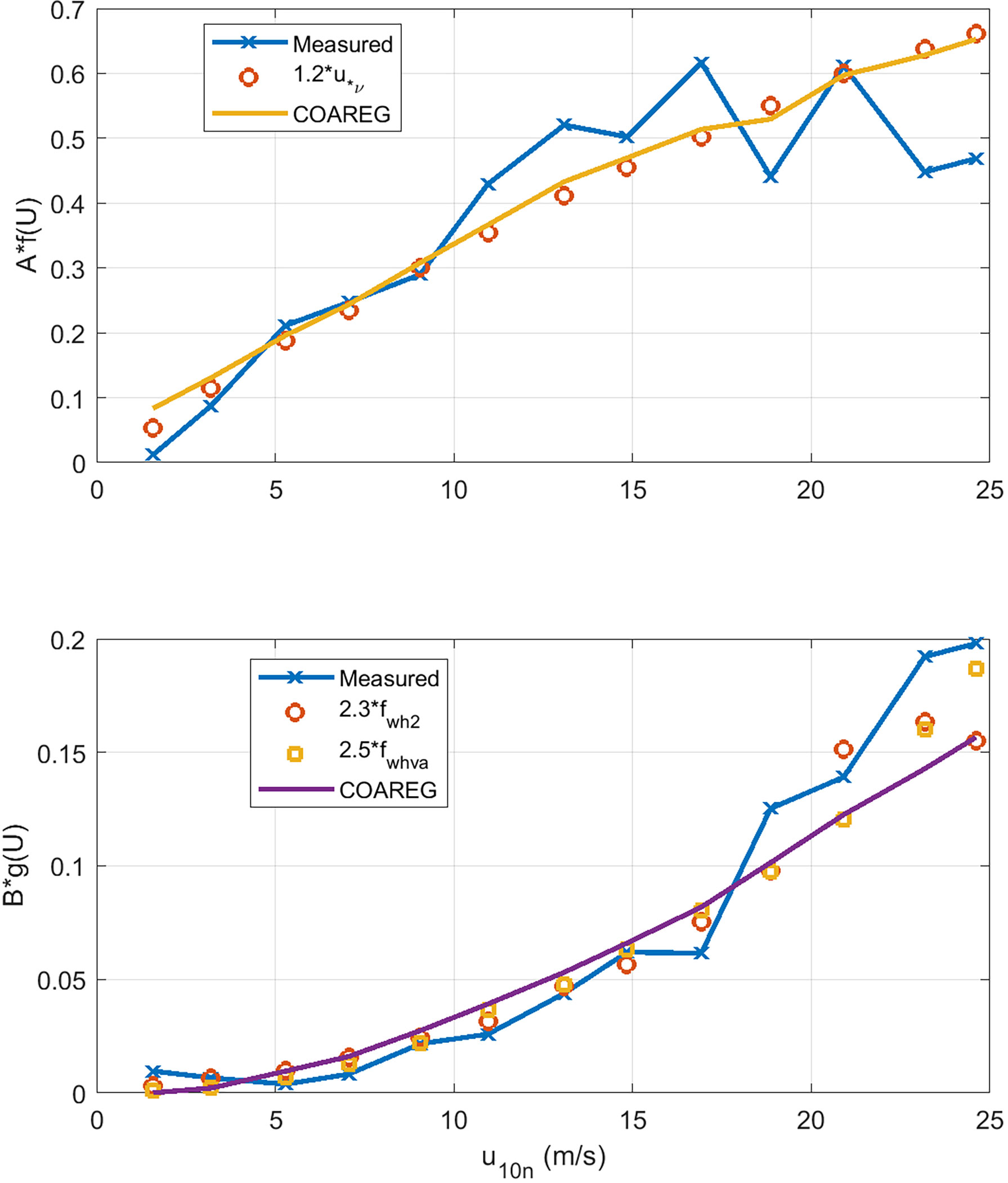
Figure 8 Extraction of wind speed dependence of the turbo-molecular (upper panel) and bubble-mediated (lower panel) water-side transfer velocity terms using wind speed bin averages to the HiWinGS data. Two different whitecap formulations are used for the B term: f_wh2 is (49). and f_whva is Deike et al. (2016). The solid lines are values extracted by applying the analysis to COAREG36 outputs.

4.2 Chemical Enhancement

We can use observations of CO₂ and DMS transfer velocity to estimate CE if the difference between CO₂ and dual tracer is due to chemical enhancement only by adding a term to (46)

Taking the difference gives

We can solve (53) for CE but we expect the values of CE will be the difference between two large numbers except at low wind speeds. In order to reduce the effect of sampling uncertainty, we have added data from four additional field programs – CO₂ from GasEx98, SOAP, and Knorr11 and DMS from SO-GasEx, SOAP, and Knorr11 – to the ensemble of data and produced a grand average for CO₂ and DMS transfer velocities (see Figure 9). In the case of GasEx98, CO₂ fluxes were determined with a closed path system that lacked a drier but used a long inlet. This tends to eliminate water vapor concentration variance and may be less affected by flux cross-talk than open path sensors. For U₁₀ < 10m s^-1, the uncertainty in these averages is ±2.0 cm hr^-1 for CO₂ and ±0.4 cm hr^-1 for DMS. The uncertainty in Δk is essentially that of CO₂. In Figure 10 we show Δk as a function of U₁₀ with separate curves for mean and medians of the four-experiment ensemble; we also show the bubble driven component [second term on RHS of (53)]. The data clearly imply values of CE on the order 4-6 cm hr^-1 at the lowest wind speeds but even at U₁₀ = 5 ms^-1 it is doubtful the difference between observations of Δk and the estimates of the bubble component are significant. This result is similar to (Yang et al., 2022) who computed a grand-averaged k_c660 from eight field programs (including the ones used here) and estimate CE by differencing their average with dual tracer estimates of k_c660 (Ho et al., 2006). Because the dual tracer studies are done with non-reactive gases, the argument is that they do not include CO₂ CE. Yang et al. (2022) found CE values of about 4 cm hr^-1 for U₁₀ < 10m s^-1. These results suggest τ_r on the order of 3 s (a_r = 0.33) should be used in (38) to estimate CE if the difference between CO₂ and dual tracer is due to chemical enhancement only.

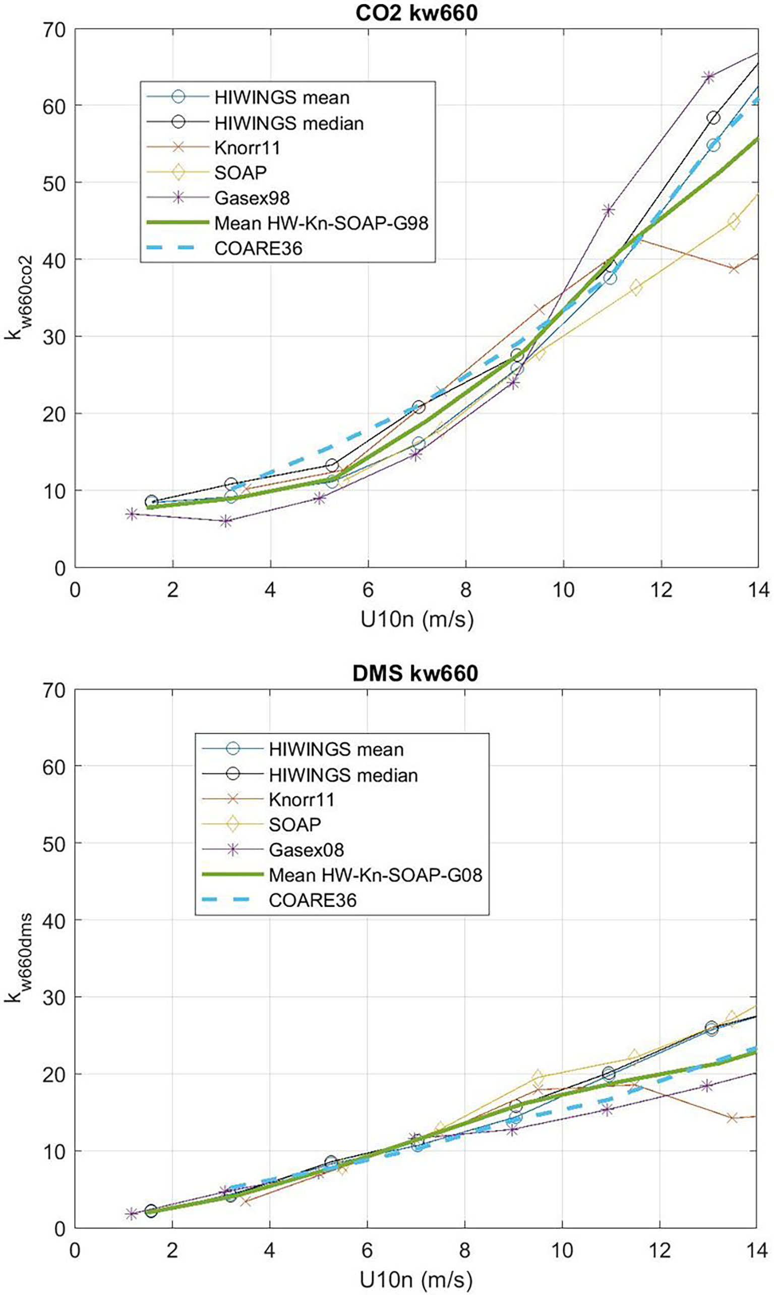
Figure 9 Wind speed bin-averaged k_w660 from HiWinGS, Knorr11, SOAP, GasEx98 and GasEx08 field programs: upper panel for CO₂ and lower panel for DMS. Both mean and median are shown for HiWinGS. The heavy green line is the mean of the five estimates. The dashed line is the COARE36 relationship.

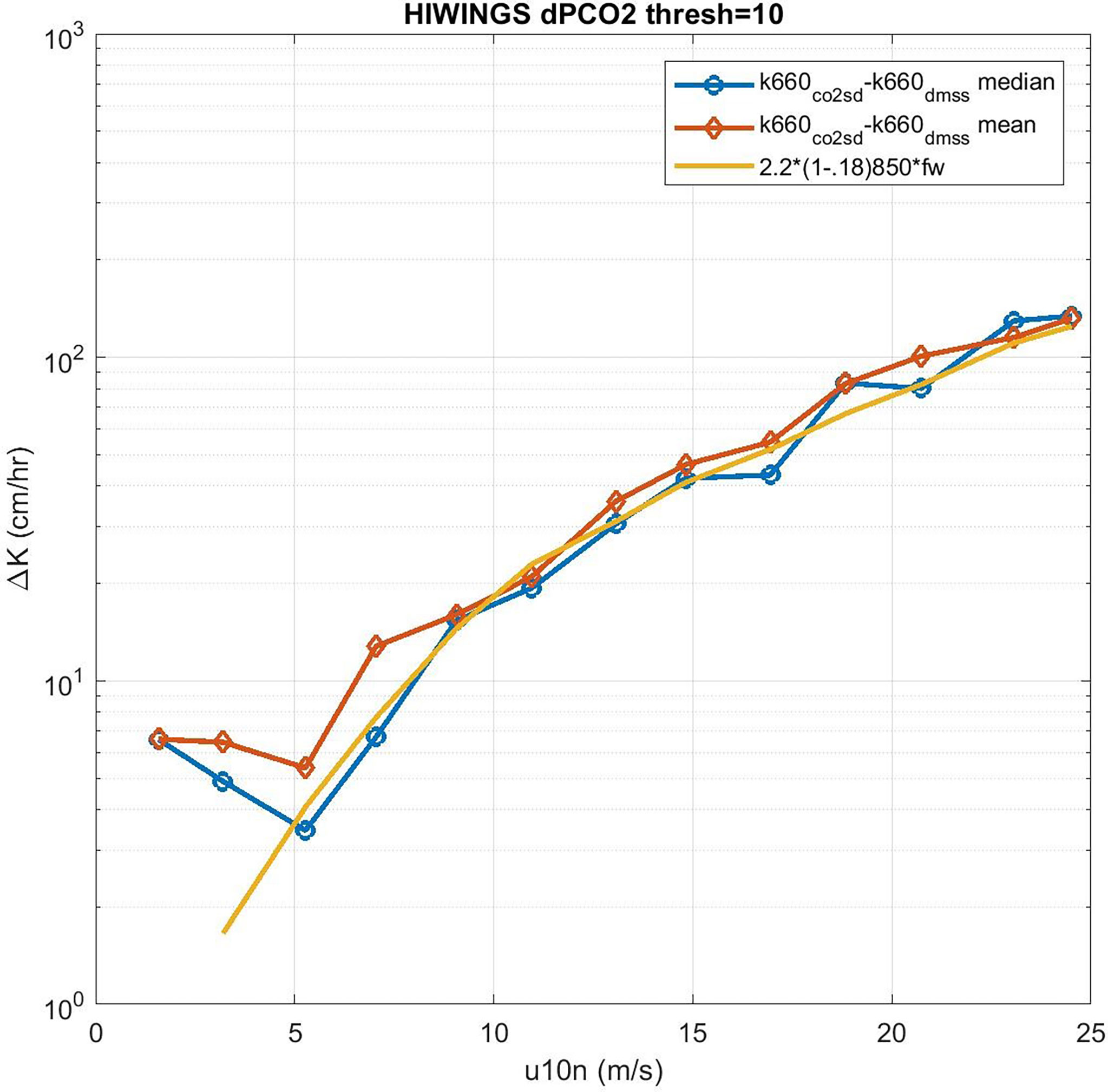
Figure 10 Difference in CO₂ and DMS transfer velocities (normalized to Sc = 660) as a function of 10-m wind speed: blue –median and red –mean. The difference of either the red or blue curves from the COAREG estimate of the residual bubble component is hypothesized to be chemical enhancement.

5 Discussion and Conclusions

In this paper we analyze concurrent observations of CO₂ and DMS fluxes and ocean-side transfer velocity from three recent field programs. We emphasize the HiWinGS program because it has the broadest range of wind speeds and multiple systems of high quality covariance flux instrumentation. We frame our analysis in terms of the COAREG gas flux algorithm, which treats the ocean-side transfer as the sum of direct interfacial and bubble-mediated transfer mechanisms. We assume the interfacial transfer component scales as the square root of the Schmidt number and is driven linearly by the viscous friction velocity. The total surface stress is partitioned into viscous and wave contributions with the fraction going to viscous stress decreasing with increasing wind speed. COAREG scales the bubble-mediated component with whitecap fraction (Woolf, 1993) with additional temperature-dependent sensitivity to Schmidt number and solubility. Whitecap fraction is difficult to measure so parametrizations are uncertain, but whitecap fraction is only one of several possible choices to characterize the wave breaking contribution to bubble-mediated exchange (other possibilities include air entrainment rate or wave energy dissipated by breaking).

The analysis focuses on determination of the tuning constants A and B, which scale with the viscous and bubble-mediated terms. We use (47) to compute values of A and B in wind-speed bins. Note the value of A obtained from (47a) is independent of the formulation of whitecap scaling and B obtained via (47b) is independent of the formulation of the forcing of the viscous term. The wind speed dependence of A and B depends on the wind speed dependence of the forcing terms. The values of A and B determined from these data are essentially independent of wind speed for the chosen forcing: linear with u_*v and with a particular whitecap formulation. At low wind speeds, there are departures for both A and B that we associate with the effects of chemical enhancement of CO₂ transfer, which are not captured in (47). CE is discussed theoretically in section 2.4 and a parameterization is presented. In section 4.2 we exploit the difference in CO₂ and DMS transfer velocities to estimate CE – the result is noisy (Figure 10) but values are comparable to Wanninkhof (1992) and (Zheng et al., 2021).

The product of this effort is version 3.6 of the COARE flux algorithm – COAREG 3.6 which is available at https://downloads.psl.noaa.gov/BLO/Air-Sea/bulkalg/cor3_6/gasflux36/(See the Supplement to this paper for more detail on the update). The algorithm incorporates a modern whitecap formulation that allows either pure wind speed or wave-dependent scaling. Chemical enhancement for CO₂ via (38) is included as an option. Wave dependence of the stress has also been updated.

Data Availability Statement

Publicly available datasets were analyzed in this study. This data can be found here: https://downloads.psl.noaa.gov/psd3/cruises/HIWINGS_2013/Fairall_etal_2022_Frontiers_Paper/. Version 3.6 of the COARE flux algorithm (COAREG 3.6) is available at: https://downloads.psl.noaa.gov/BLO/Air-Sea/bulkalg/cor3_6/gasflux36/.

Author Contributions

CWF wrote the first draft of the manuscript, MY and SEB each contributed a subsection. CWF, BWB, and MY revised the manuscript following the peer review process. JBE, CJZ, TGB, ESS, and SEB participated in discussions and provided edits. CWF, BWB, MY, SEB, LB, and CJZ participated in the HiWinGS experiment. TGB and ESS participated in the Knorr11 and SOAP experiment. JBE, CWF, and CJZ participated in the GasEx98 experiment. BB, LB, JBE, and CJZ participated in the SO-GasEx experiment. LB performed the numerical simulations with DE equation solver. SP and LB provided technical support for instrumentation, data collection, and analysis. All authors read and approved the finalized version.

Funding

This work, and the contributions of MY and TB, is supported by the UK Natural Environment Research Council’s ORCHESTRA (Grant No. NE/N018095/1) and PICCOLO (Grant No. NE/P021409/1) projects, and by the European Space Agency’s AMT4OceanSatFlux project (Grant No. 4000125730/18/NL/FF/gp). CF and BB are funded by the National Oceanic and Atmospheric Administration’s Global Ocean Monitoring and Observing program (http://data.crossref.org/fundingdata/funder/10.13039/100018302). CZ was funded by the National Science Foundation (CJZ: OCE-2049579, Grants OCE-1537890 and OCE-1923935). Funding for HiWinGS was provided by the US National Science Foundation grant AGS-1036062. The Knorr-11 and SOAP campaigns were supported by the NSF Atmospheric Chemistry Program (Grant No. ATM-0426314, AGS-08568, -0851472, -0851407 and -1143709).

Conflict of Interest

The authors declare that the research was conducted in the absence of any commercial or financial relationships that could be construed as a potential conflict of interest.

Publisher’s Note

All claims expressed in this article are solely those of the authors and do not necessarily represent those of their affiliated organizations, or those of the publisher, the editors and the reviewers. Any product that may be evaluated in this article, or claim that may be made by its manufacturer, is not guaranteed or endorsed by the publisher.

Acknowledgments

SB was supported by a postdoctoral grant from the Centre National d’Études Spatiales (CNES).

Supplementary Material

The Supplementary Material for this article can be found online at: https://www.frontiersin.org/articles/10.3389/fmars.2022.826606/full#supplementary-material

References

Andersson A., Falck E., Sjöblom A., Kljun N., Sahlée E., Omar A. M., et al. (2017). Air-Sea Gas Transfer in High Arctic Fjords. Geophysical Res. Lett. 44, 2519–2526. doi: 10.1002/2016GL072373
Anguelova M. D., Bettenhausen M. H. (2019). Whitecap Fraction From Satellite Measurements: Algorithm Description. J. Geophysical Research: Oceans 124, 1827–1857. doi: 10.1029/2018JC014630
Bell T. G., De Bruyn W., Miller S. D., Ward B., Christensen K., Saltzman E. S. (2013). Air-Sea Dimethylsulfide (DMS) Gas Transfer in the North Atlantic: Evidence for Limited Interfacial Gas Exchange at High Wind Speed. Atmospheric Chem. Phys. 13, 11073–11087. doi: 10.5194/acp-13-11073-2013
Bell T. G., Landwehr S., Miller S. D., de Bruyn W. J., Callaghan A., Scanlon B., et al. (2017). Estimation of Bubbled-Mediated Air/Sea Gas Exchange From Concurrent DMS and CO2 Transfer Velocities at Intermediate-High Wind Speeds. Atmos. Chem. Phys. Discuss. 2017, 1–29. doi: 10.5194/acp-2017-85
Blomquist B. W., Brumer S. E., Fairall C. W., Huebert B. J., Zappa C. J., Brooks I. M., et al. (2017). Wind Speed and Sea State Dependencies of Air-Sea Gas Transfer: Results From the High Wind Speed Gas Exchange Study (HiWinGS). J. Geophysical Research: Oceans 122, 8034–8062. doi: 10.1002/2017JC013181
Blomquist B. W., Fairall C. W., Huebert B. J., Kieber D. J., Westby G. R. (2006). Dms Sea-Air Transfer Velocity: Direct Measurements by Eddy Covariance and Parameterization Based on the NOAA/COARE Gas Transfer Model. Geophysical Res. Lett. 33, L07601. doi: 10.1029/2006GL025735
Blomquist B. W., Huebert B. J., Fairall C. W., Bariteau L., Edson J. B., Hare J. E., et al. (2014). Advances in Air-Sea CO2 Flux Measurement by Eddy Correlation. Boundary-Layer Meteorology 152, 245–276. doi: 10.1007/s10546-014-9926-2
Blomquist B. W., Huebert B. J., Fairall C. W., Faloona I. C. (2010). Determining the Sea-Air Flux of Dimethylsulfide by Eddy Correlation Using Mass Spectrometry. Atmospheric Measurement Techniques 3, 1–20. doi: 10.5194/amt-3-1-2010
Brumer S. E., Zappa C. J., Blomquist B. W., Fairall C. W., Cifuentes-Lorenzen A., Edson J. B., et al. (2017a). Wave-Related Reynolds Number Parameterizations of CO2 and DMS Transfer Velocities. Geophysical Res. Lett. 44, 9865–9875. doi: 10.1002/2017GL074979
Brumer S. E., Zappa C. J., Brooks I. M., Tamura H., Brown S. M., Blomquist B., et al. (2017b). Whitecap Coverage Dependence on Wind and Wave Statistics as Observed During SO-GasEx and HiWinGS. J. Phys. Oceanography 47(9); 2211–2235. doi: 10.1175/JPO-D-17-0005.1
Butterworth B. J., Miller S. D. (2016). Air-Sea Exchange of Carbon Dioxide in the Southern Ocean and Antarctic Marginal Ice Zone. Geophysical Res. Lett. 43, 7223–7230. doi: 10.1002/2016GL069581
Callaghan A. H. (2013). An Improved Whitecap Timescale for Sea Spray Aerosol Production Flux Modeling Using the Discrete Whitecap Method. J. Geophysical Research: Atmospheres 118, 9997–10010. doi: 10.1002/jgrd.50768
Callaghan A. H. (2018). On the Relationship Between the Energy Dissipation Rate of Surface-Breaking Waves and Oceanic Whitecap Coverage. J. Phys. Oceanography 48, 2609–2626. doi: 10.1175/JPO-D-17-0124.1
Callaghan A. H., Deane G. B., Stokes M. D. (2016). Laboratory Air-Entraining Breaking Waves: Imaging Visible Foam Signatures to Estimate Energy Dissipation. Geophysical Res. Lett. 43 (11), 320–11,328. doi: 10.1002/2016GL071226
Cifuentes-Lorenzen A., Edson J. B., Zappa C. J. (2018). Air-Sea Interaction in the Southern Ocean: Exploring the Height of the Wave Boundary Layer at the Air-Sea Interface. Boundary-Layer Meteorology 169, 461–482. doi: 10.1007/s10546-018-0376-0
Cronin M. F., Gentemann C. L., Edson J., Ueki I., Bourassa M., Brown S., et al. (2019). Air-Sea Fluxes With a Focus on Heat and Momentum. Front. Mar. Sci. 6. doi: 10.3389/fmars.2019.00430
Deike L., Lenain L., Melville W. K. (2017). Air Entrainment by Breaking Waves. Geophysical Res. Lett. 44, 3779–3787. doi: 10.1002/2017GL072883
Deike L., Melville W. K. (2018). Gas Transfer by Breaking Waves. Geophysical Res. Lett. 45 (10), 482–10,492. doi: 10.1029/2018GL078758
Deike L., Melville W. K., Popinet S. (2016). Air Entrainment and Bubble Statistics in Breaking Waves. J. Fluid Mechanics 801, 91–129. doi: 10.1017/jfm.2016.372
Dong Y., Yang M., Bakker D. C. E., Kitidis V., Bell T. G. (2021). Uncertainties in Eddy Covariance Air–Sea CO2 Flux Measurements and Implications for Gas Transfer Velocity Parameterisations. Atmospheric Chem. Phys. 21, 8089–8110. doi: 10.5194/acp-21-8089-2021
Edson J. B., Fairall C. W., Bariteau L., Zappa C. J., Cifuentes-Lorenzen A., McGillis W. R., et al. (2011). Direct Covariance Measurement of CO2 Gas Transfer Velocity During the 2008 Southern Ocean Gas Exchange Experiment: Wind Speed Dependency. J. Geophysical Res. - Oceans 116, C00F. doi: 10.1029/2011JC007022
Edson J. B., Hinton A. A., Prada K. E., Hare J. E., Fairall C. W. (1998). Direct Covariance Flux Estimates From Mobile Platforms at Sea. J. Atmospheric Oceanic Technol. 15, 547–562. doi: 10.1175/1520-0426(1998)015<0547:DCFEFM>2.0.CO;2
Edson J. B., Jampana V., Weller R. A., Bigorre S. P., Plueddemann A. J., Fairall C. W. (2013). On the Exchange of Momentum Over the Open Ocean. J. Phys. Oceanography 43, 1589–1610. doi: 10.1175/JPO-D-12-0173.1
Edson J. B., Zappa C. J., Ware J., McGillis W. R., Hare J. E. (2004). Scalar Flux Profile Relationships Over the Open Ocean. J. Geophys. Res. 109, C08S09. doi: 10.1029/2003JC001960
Esters L., Landwehr S., Sutherland G., Bell T. G., Christensen K. H., Saltzman E. S., et al. (2017). Parameterizing Air-Sea Gas Transfer Velocity With Dissipation. J. Geophysical Research: Oceans 122, 3041–3056. doi: 10.1002/2016JC012088
Fairall C. W., Bradley E. F., Hare J. E., Grachev A. A., Edson J. B. (2003). Bulk Parameterization of Air-Sea Fluxes: Updates and Verification for the Coare Algorithm. J. Climate 16, 571–591. doi: 10.1175/1520-0442(2003)016<0571:BPOASF>2.0.CO;2
Fairall C. W., Bradley E. F., Rogers D. P., Edson J. B., Young G. S. (1996). Bulk Parameterization of Air-Sea Fluxes for Tropical Ocean Global Atmosphere Coupled Ocean Atmosphere Response Experiment. J. Of Geophysical Res. 101, 3747–3764. doi: 10.1029/95JC03205
Fairall C. W., Hare J., Edson J., McGillis W. (2000). Parameterization and Micrometeorological Measurement of Air-Sea Gas Transfer. Bound.-Layer Meteor. 96, 63–105. doi: 10.1023/A:1002662826020
Fairall C. W., Helmig D., Ganzeveld L., Hare J. (2007). Water-Side Turbulence Enhancement of Ozone Deposition to the Ocean. Atmospheric Chem. Phys. 7, 443–451. doi: 10.5194/acp-7-443-2007
Fairall C. W., Yang M., Bariteau L., Edson J. B., Helmig D., McGillis W., et al. (2011). Implementation of the Coupled Ocean-Atmosphere Response Experiment Flux Algorithm With CO2, Dimethyl Sulfide, and O2. J. Geophysical Res. 116, C00F09. doi: 10.1029/2010JC006884
Flügge M., Paskyabi M. B., Reuder J., Edson J. B., Plueddemann A. J. (2016). Comparison of Direct Covariance Flux Measurements From an Offshore Tower and a Buoy. J. Atmospheric Oceanic Technol. 33, 873–890. doi: 10.1175/JTECH-D-15-0109.1
Garbe C. S., Rutgersson A., Boutin J., Leeuw G., Delille B., Fairall C. W., et al. (2014). Transfer Across the Air-Sea Interface (Springer Berlin, Heidelberg, New York: Springer Earth System Sciences). 55–112. doi: 10.1007/978-3-642-25643-1
Ghobadian M., Stammer D. (2019). Inferring Air-Sea Carbon Dioxide Transfer Velocities From Sea Surface Scatterometer Measurements. J. Geophysical Research: Oceans 124, 7974–7988. doi: 10.1029/2019JC014982
Goddijn-Murphy L., Woolf D. K., Callaghan A. H., Nightingale P. D., Shutler J. D. (2016). A Reconciliation of Empirical and Mechanistic Models of the Air-Sea Gas Transfer Velocity. J. Geophysical Research: Oceans 121, 818–835. doi: 10.1002/2015JC011096
Gutiérrez-Loza L., Wallin M. B., Sahlée E., Nilsson E., Bange H. W., Kock A., et al. (2019). Measurement of Air-Sea Methane Fluxes in the Baltic Sea Using the Eddy Covariance Method. Front. Earth Sci. 7. doi: 10.3389/feart.2019.00093
Ho D. T., Law C. S., Smith M. J., Schlosser P., Harvey M., Hill P. (2006). Measurements of Air-Sea Gas Exchange at High Wind Speeds in the Southern Ocean: Implications for Global Parameterizations. Geophys. Res. Lett. 33, L16611. doi: 10.1029/2006GL026817
Hoover T. E., Berkshire D. C. (1969). Effects of Hydration on Carbon Dioxide Exchange Across an Air-Water Interface. J. Geophysical Res. 74, 456–464. doi: 10.1029/JB074i002p00456
Ho D., Sabine C. L., Hebert D., Ullman D. S., Wanninkhof R., Hamme R. C., et al. (2011). Southern Ocean Gas Exchange Experiment: Setting the Stage. J. Geophysical Res. - Oceans 116, C00F08. doi: 10.1029/2010JC006852
Jørgensen H. E., Sørensen L. L., Larsen S. E. (2020). A Simple Model of Chemistry Effects on the Air-Sea CO2 Exchange Coefficient. J. Geophysical Research: Oceans 125, e2018JC014808. doi: 10.1029/2018JC014808
Johnson M. T. (2010). A Numerical Scheme to Calculate Temperature and Salinity Dependent Air-Water Transfer Velocities for Any Gas. Ocean Sci. 6, 913–932. doi: 10.5194/os-6-913-2010
Johnson K. S., Barry J. P., Coletti L. J., Fitzwater S. E., Jannasch H. W., Lovera C. F. (2011). Nitrate and Oxygen Flux Across the Sediment-Water Interface Observed by Eddy Correlation Measurements on the Open Continental Shelf. Limnology Oceanography: Methods 9, 543–553. doi: 10.4319/lom.2011.9.543
Krall K. E., Smith A. W., Takagaki N., Jähne B. (2019). Air–sea Gas Exchange at Wind Speeds Up to 85 ms-1. Ocean Sci. 15, 1783–1799. doi: 10.5194/os-15-1783-2019
Landwehr S., Miller S. D., Smith M. J., Bell T. G., Saltzman E. S., Ward B. (2018). Using Eddy Covariance to Measure the Dependence of Air–Sea CO2 Exchange Rate on Friction Velocity. Atmospheric Chem. Phys. 18, 4297–4315. doi: 10.5194/acp-18-4297-2018
Landwehr S., Miller S. D., Smith M. J., Saltzman E. S., Ward B. (2014). Analysis of the PKT Correction for Direct CO2 Flux Measurements Over the Ocean. Atmospheric Chem. Phys. 14, 3361–3372. doi: 10.5194/acp-14-3361-2014
Landwehr S., O’Sullivan N., Ward B. (2015). Direct Flux Measurements From Mobile Platforms at Sea: Motion and Air-Flow Distortion Corrections Revisited. J. Atmospheric Oceanic Technol 32(6); 1163–1178. doi: 10.1175/JTECH-D-14-00137.1
Liang J.-H., Deutsch C., McWilliams J. C., Baschek B., Sullivan P. P., Chiba D. (2013). Parameterizing Bubble-Mediated Air-Sea Gas Exchange and its Effect on Ocean Ventilation. Global Biogeochemical Cycles 27, 894–905. doi: 10.1002/gbc.20080
Liss P. S., Merlivat L. (1986). Air-Sea Gas Exchange Rates: Introduction and Synthesis (Dordrecht, Holland: D. Reidel), 113–127.
Liss P. S., Slater P. G. (1974). Flux of Gases Across the Air-Sea Interface. Nature 247, 181–184. doi: 10.1038/247181a0
Luhar A. K., Woodhouse M. T., Galbally I. E. (2018). A Revised Global Ozone Dry Deposition Estimate Based on a New Two-Layer Parameterisation for Air–Sea Exchange and the Multi-Year Macc Composition Reanalysis. Atmospheric Chem. Phys. 18, 4329–4348. doi: 10.5194/acp-18-4329-2018
McGillis W. R., Wanninkhof R. (2006). Aqueous CO2 Gradients for Air-Sea Flux Estimates. Mar. Chem. 98, 100–108. doi: 10.1016/j.marchem.2005.09.003
Melville W. K. (1996). The Role of Surface-Wave Breaking in Air-Sea Interaction. Annu. Rev. Fluid Mechanics 28, 279–321. doi: 10.1146/annurev.fl.28.010196.001431
Miller S. D., Marandino C., Saltzman E. S. (2010). Ship-Based Measurement of Air-Sea CO2 Exchange by Eddy Covariance. J. Geophysical Research: Atmospheres 115, D02304. doi: 10.1029/2009JD012193
Monahan E. C. (1971). Oceanic Whitecaps. J. Phys. Oceanography 1, 139–144. doi: 10.1175/1520-0485(1971)001<0139:OW>2.0.CO;2
Ortiz-Suslow D. G., Kalogiros J., Yamaguchi R., Wang Q. (2021). An Evaluation of the Constant Flux Layer in the Atmospheric Flow Above the Wavy Air-Sea Interface. J. Geophysical Research: Atmospheres 126, e2020JD032834. doi: 10.1029/2020JD032834
Porter J. G., de Bruyn W. J., Miller S. D., Saltzman E. S. (2020). Air/sea Transfer of Highly Soluble Gases Over Coastal Waters. Geophysical Res. Lett. 47, e2019GL085286. doi: 10.1029/2019GL085286
Porter J. G., De Bruyn W., Saltzman E. S. (2018). Eddy Flux Measurements of Sulfur Dioxide Deposition to the Sea Surface. Atmospheric Chem. Phys. 18, 15291–15305. doi: 10.5194/acp-18-15291-2018
Prytherch J., Brooks I. M., Crill P. M., Thornton B. F., Salisbury D. J., Tjernström M., et al. (2017). Direct Determination of the Air-Sea CO2 Gas Transfer Velocity in Arctic Sea Ice Regions. Geophysical Res. Lett. 44, 3770–3778. doi: 10.1002/2017GL073593
Prytherch J., Yelland M. (2021). Wind, Convection and Fetch Dependence of Gas Transfer Velocity in an Arctic Sea-Ice Lead Determined From Eddy Covariance CO2 Flux Measurements. Global Biogeochemical Cycles 35, e2020GB006633. doi: 10.1029/2020GB006633
Rhee T. S., Nightingale P. D., Woolf D. K., Caulliez G., Bowyer P., Andreae M. O. (2007). Influence of Energetic Wind and Waves on Gas Transfer in a Large Wind-Wave Tunnel Facility. J. Geophysical Res. 112, C05027. doi: 10.1029/2005JC003358
Rowe M. D., Fairall C. W., Perlinger J. A. (2011). Chemical Sensor Resolution Requirements for Near-Surface Measurements of Turbulent Fluxes. Atmos. Chem. Phys. 11, 5263–5275. doi: 10.5194/acp-11-5263-2011
Rutgersson A., Pettersson H., Nilsson E., Bergström H., Wallin M. B., Nilsson E. D., et al. (2020). Using Land-Based Stations for Air-Sea Interaction Studies. Tellus A: Dynamic Meteorology Oceanography 72, 1–23. doi: 10.1080/16000870.2019.1697601
Shutler J. D., Land P. E., Piolle J.-F., Woolf D. K., Goddijn-Murphy L., Paul F., et al. (2016). FluxEngine: A Flexible Processing System for Calculating Atmosphere-Ocean Carbon Dioxide Gas Fluxes and Climatologies. J. Atmospheric Oceanic Technol. 33, 741–756. doi: 10.1175/JTECH-D-14-00204.1
Shutler J. D., Wanninkhof R., Nightingale P. D., Woolf D. K., Bakker D. C. E., Watson A., et al. (2020). Satellites Will Address Critical Science Priorities for Quantifying Ocean Carbon. Front. Ecol. Environ. 18, 27–35. doi: 10.1002/fee.2129
Soloviev A. V. (2007). Coupled Renewal Model of Ocean Viscous Sublayer, Thermal Skin Effect and Interfacial Gas Transfer Velocity. J. Mar. Syst. 66, 19–27. doi: 10.1016/j.jmarsys.2006.03.024
Vieira V., Mateus M., Canelas R., Leitão F. (2020). The Fugas 2.5 Updated for the Effects of Surface Turbulence on the Transfer Velocity of Gases at the Atmosphere-Ocean Interface. J. Mar. Sci. Eng. 8, 435. doi: 10.3390/jmse8060435
Wanninkhof R. (1992). Relationship Between Wind Speed and Gas Exchange Over the Ocean. J. Geophysical Res. 97, 7373–7382. doi: 10.1029/92JC00188
Wanninkhof R. (2014). Relationship Between Wind Speed and Gas Exchange Over the Ocean Revisited. Limnology Oceanography: Methods 12, 351–362. doi: 10.4319/lom.2014.12.351
Wanninkhof R., Asher W. E., Ho D., Sweeney C., McGillis W. (2009). Advances in Quantifying Air-Sea Gas Exchange and Environmental Forcing. Annu. Rev. Mar. Sci. 1, 213–244. doi: 10.1146/annurev.marine.010908.163742
Wanninkhof R., Knox M. (1996). Chemical Enhancement of CO2 Exchange in Natural Waters. Limnol. Oceanogr. 41, 689–697. doi: 10.4319/lo.1996.41.4.0689
Woolf D. K. (1993). Bubbles and the Air-Sea Transfer Velocity of Gases. Atmos. Ocean 31, 517–540. doi: 10.1080/07055900.1993.9649484
Woolf D., Shutler J., Goddijn-Murphy L., Watson A., Chapron B., Nightingale P., et al. (2019). Key Uncertainties in the Recent Air-Sea Flux of CO2. Global Biogeochemical Cycles 33, 1548–1563. doi: 10.1029/2018GB006041
Woolf D. K., Thorpe S. A. (1991). Bubbles and the Air-Sea Exchange of Gases in Near Saturation Conditions. J. Mar. Res. 49, 435–466. doi: 10.1357/002224091784995765
Yang M., Bell T. G., Bidlot J., Blomquist B. W., Butterworth B. J., Dong Y., et al. (2022). Global Synthesis of Air-Sea CO2 Transfer Velocity Estimates From Ship-Based Eddy Covariance Measurements. Front. Mar. Sci. Sec. Ocean Observation. doi: 10.3389/fmars.2022.826421
Yang M., Bell T. G., Hopkins F. E., Kitidis V., Cazenave P. W., Nightingale P. D., et al. (2016). Air–sea Fluxes of CO2 and CH4 From the Penlee Point Atmospheric Observatory on the South-West Coast of the UK. Atmospheric Chem. Phys. 16, 5745–5761. doi: 10.5194/acp-16-5745-2016
Yang M., Blomquist B., Nightingale P. D. (2014). Air-Sea Exchange of Methanol and Acetone During Hiwings: Estimation of Air Phase, Water Phase Gas Transfer Velocities. J. Geophysical Research: Oceans 119, 7308–7323. doi: 10.1002/2014JC010227
Yang M., Norris S. J., Bell T. G., Brooks I. M. (2019). Sea Spray Fluxes From the Southwest Coast of the United Kingdom–Dependence on Wind Speed and Wave Height. Atmospheric Chem. Phys. 19, 15271–15284. doi: 10.5194/acp-19-15271-2019
Zavarsky A., Goddijn-Murphy L., Steinhoff T., Marandino C. A. (2018). Bubble-Mediated Gas Transfer and Gas Transfer Suppression of DMS and CO2. J. Geophysical Research: Atmospheres 123, 6624–6647. doi: 10.1029/2017JD028071
Zavarsky A., Marandino C. A. (2019). The Influence of Transformed Reynolds Number Suppression on Gas Transfer Parameterizations and Global DMS and CO2 Fluxes. Atmospheric Chem. Phys. 19, 1819–1834. doi: 10.5194/acp-19-1819-2019
Zheng T., Feng S., Davis K. J., Pal S., Morguí J.-A. (2021). Development and Evaluation of CO2 Transport in Mpas-a V6.3. Geoscientific Model. Dev. 14, 3037–3066. doi: 10.5194/gmd-14-3037-2021
Keywords: gas transfer velocity, chemical enhancement, bubble mediated transfer, COARE gas flux parameterization, Dimethylsufide (DMS), cardon dioxide (CO2), bulk algorithm, direct observation
Citation: Fairall CW, Yang M, Brumer SE, Blomquist BW, Edson JB, Zappa CJ, Bariteau L, Pezoa S, Bell TG and Saltzman ES (2022) Air-Sea Trace Gas Fluxes: Direct and Indirect Measurements. Front. Mar. Sci. 9:826606. doi: 10.3389/fmars.2022.826606
Received: 01 December 2021; Accepted: 24 May 2022;
Published: 29 July 2022.
Edited by:
Petra Heil, Australian Antarctic Division, AustraliaReviewed by:
Sohiko Kameyama, Hokkaido University, JapanIvan Mammarella, University of Helsinki, Finland
Copyright © 2022 Fairall, Yang, Brumer, Blomquist, Edson, Zappa, Bariteau, Pezoa, Bell and Saltzman. This is an open-access article distributed under the terms of the Creative Commons Attribution License (CC BY). The use, distribution or reproduction in other forums is permitted, provided the original author(s) and the copyright owner(s) are credited and that the original publication in this journal is cited, in accordance with accepted academic practice. No use, distribution or reproduction is permitted which does not comply with these terms.
*Correspondence: Christopher W. Fairall, chris.fairall@noaa.gov