Sound Scattering Layers Within and Beyond the Seychelles-Chagos Thermocline Ridge in the Southwest Indian Ocean

Introduction

Marine biomes account for approximately 71% of the Earth′s surface. One of the most remarkable features of this biome is the presence of ubiquitous and persistent sound scattering layers (SL). The sound SL appear continuous on the echogram from an echosounder, vertically narrow, tens to hundreds of meters, and horizontally extensive for tens to thousands of kilometers (Simmonds and MacLennan, 2005). Generally, they consist of two types of layers: the shallow scattering layer, which is found from the sea surface to 200 m deep in the epipelagic zone, and the deep scattering layer, which is detected from 200 to 1,000 m in the mesopelagic zone (Ariza et al., 2016; Proud et al., 2017; Gjøsæter et al., 2020). Often, there is more than one scattering layer. The morphology and backscattering strength of the SL vary globally (Klevjer et al., 2016; Knutsen et al., 2017; Proud et al., 2017; Annasawmy et al., 2018). The SL is composed of broad taxonomic groups and typically ranges in size from 1 to 20 cm (Kloser et al., 2009).

Most SL organisms carry out extensive diel vertical migration (DVM), which is the Earth’s largest animal migration in the epipelagic (0–200 m) and mesopelagic (200–1,000 m) zones, and they migrate through different depths in the water column daily. The DVM includes nocturnal vertical migration, where SL organisms ascend to the surface layers from deep layers around dusk, remain at the surface for the night, and then migrate back to the depth around dawn. Although the mesopelagic zone has been labeled as the twilight zone of the water layers, there is sufficient downwelling irradiance for visual detection of prey, but not for photosynthesis during the daytime (Ramirez–Llodra et al., 2010). Several species prey on SL organisms, such as ocean nekton, including tuna and billfish, seabirds, and marine mammals (Boersch–Supan et al., 2017; Sato and Benoit–Bird, 2017). In marine food webs, they are a key trophic link between primary consumers and commercially valuable species, as well as predators on the top of the food web (Danckwerts et al., 2014; Jaquemet et al., 2014; Cherel et al., 2020). They serve as a vehicle for the transfer of energy to deeper layers of the ocean through respiration, excretion, fecal pellet production, and natural mortality (Catul et al., 2011; Bianchi et al., 2013). The DVM of SL organisms plays a substantial role in the biogeochemical cycles, including the biological pump, by transporting carbon from productive upper layers to less productive deeper layers (Spear et al., 2007; Bianchi et al., 2013). They supply substantial nutrients and particulate organic matter downward in the water column. The onset of DVM is believed to result from various factors. For example, exogenous factors, including light penetration and intensity, the phase of the moon, temperature, oxygen concentration, productivity, and oceanographic and bathymetric features are thought to influence the distribution and behavior of migrants (Davison et al., 2015; Klevjer et al., 2016; Aksnes et al., 2017; Proud et al., 2017; Langbehn et al., 2019; Annasawmy et al., 2020; Bernal et al., 2020; Boswell et al., 2020). Endogenous factors such as age, size, energetic state, and behavioral and physiological properties also influence migration (Ringelberg, 1995; Yasuma et al., 2010).

Micronekton are the dominant component of the SL organisms that inhabit the twilight zone, and they account for a significant proportion of DVM that feed on zooplankton near the surface. Their distribution can vary considerably depending on the time of day, area, season, and water mass characteristics (Prihartato et al., 2015; Annasawmy et al., 2019; Geoffroy et al., 2019; Cisewski et al., 2021). They are considered a potential harvestable resource because of their huge biomass and nutritional quality (protein and marine lipids), and some species can be suitable food sources for humans. Although they have mostly been supplied as raw material to the fish meal and oil industry, interest in their commercial exploitation is increasing (Grimaldo et al., 2020). Among micronekton, mesopelagic fishes (myctophiformes) are extraordinarily abundant in all oceans worldwide (Kaartvedt et al., 2012). In particular, myctophids account for up to 75% of the total global catch of mesopelagic fishes and are considered the most abundant vertebrate species on the planet (Shilat and Valinassab, 1998). Historically, global biomass estimates of myctophids using net sampling were 10,000 million metric tons (Gjøsaeter and Kawaguchi, 1980). However, a macroecological model and a recent simple food-web model estimated 2.4 and 1.4 billion metric tons, respectively (Jennings and Collingridge, 2015; Anderson et al., 2019). Additionally, the greatest estimated biomass was 11–15 billion metric tons using 38 kHz acoustic data (Irigoien et al., 2014). Overall, the worldwide biomass of mesopelagic fishes is enormous, although it varies substantially. The difference of 1–2 orders of magnitude could be due to the selectivity of fishing gears and non-linear acoustic resonance scattering with fish size. As mentioned earlier, SL organisms have high species diversity. Accordingly, to identify their species and measure their sizes, a net sampling method may not be adequate. Apart from species diversity, they inhabit an extremely broad range of water depths, which further makes net sampling challenging. Additionally, it is nearly impossible to estimate accurate biomass values from acoustic data alone. Nevertheless, acoustic backscatter data from multiple frequencies can provide meaningful behavioral and ecological information (D’Elia et al., 2016; Kang et al., 2016, 2020; Béhagle et al., 2017).

The southwest Indian Ocean has a unique feature, known as the Seychelles-Chagos Thermocline Ridge (SCTR; Vialard et al., 2009), also called the thermocline dome or the Seychelles dome (McCreary et al., 1993; Yokoi et al., 2008). Unlike in the Pacific and Atlantic Oceans, where easterly trade winds drive equatorial upwelling, the monsoon-dominated Indian Ocean has the off-equatorial center of upwelling due to westerly winds rather than easterly winds along the equator and southeasterly trade winds (Schott et al., 2009; Wang and McPhaden, 2017). The off-equatorial upwelling is characterized by a relatively thin surface mixed layer and shallow thermocline across the southern tropical Indian Ocean and is referred to as the SCTR. The SCTR is a region (5–12°S, 55–90°E) with significant thermocline upwelling, which is strongly linked to intraseasonal, interannual, and decadal climate variability, such as the Madden-Julian Oscillation (MJO), Indian Ocean Dipole (IOD), El Niño Southern Oscillation (ENSO), and consequent ecosystem-biogeochemical variability (Li et al., 2014; Burns and Subrahmanyam, 2016; D’Addezio and Subrahmanyam, 2018). The SCTR often hosts the origin of MJO associated with strong variability of sea surface temperature (SST) and presents high climate variability during ENSO and IOD events, resulting in major anomalies in ocean-atmosphere interaction processes such as aberrant rainfall in East Africa, tropical cyclone characteristics, and the onset of the Indian monsoon (Yokoi et al., 2008). The SCTR is important for biogeochemical cycles that affect upper ocean nutrients and relevant marine organisms. The upwelling of deeper, colder, and nourishing water affects plankton and micronekton. Nutrients in the surface layer during the monsoon seasons contribute to the growth of phytoplankton blooms twice a year, resulting in biological productivity, which is the foraging habitat for tuna species (Lan et al., 2012; Kumar et al., 2014; Marsac, 2018). Mesopelagic organisms are positioned in a critical trophic connection between primary and tertiary consumers, such as tuna, in the southwest Indian Ocean. This suggests that the life of marine organisms and environmental variables are closely associated with each other in the southwest Indian Ocean.

Despite their importance, SL organisms in the southwest Indian Ocean are poorly understood, particularly within and beyond the SCTR. Information on several aspects of their distribution dynamics, relevant marine environmental properties, and dominant species and density is lacking. A better understanding of the spatial distributional properties of SL organisms with environmental elements would be of great value in estimating micronekton biomass, calculating the budget of biological carbon pumps, modeling marine food webs or global marine ecosystems, and eventually supporting climate change adaptation. As previously mentioned, the SCTR is known to have unique oceanographic characteristics. Accordingly, it can be assumed that SL organisms within and beyond the SCTR are distributed differently. To date, no research has been conducted on SL organisms in this area.

The main goals of this study were to compare the characteristics of the SL organisms within and beyond the SCTR in consideration of (1) the identification of DVM patterns, (2) the metrics of categorized acoustic scatterers (referring to SL organisms), (3) horizontal and vertical distributional dynamics, (4) connection with environmental properties, and (5) dominant zooplankton.

Materials and Methods

Field Survey and Data Collection

Acoustic data were collected using a scientific echosounder (18, 38, 70, 120, 200, and 333 kHz of EK80, Simrad) from April 20 to May 15, 2019, in the southwest Indian Ocean using the RV Isabu (5,894 tons). Six transducers were mounted at a depth of 6 m below the water surface. To investigate the acoustic scatterers up to 1,000 m, only lower frequencies (18 and 38 kHz) were used in this study because of the effective acoustic detection range. For the parameters of the scientific echosounder, the beam angles at 18 and 38 kHz were 11.5° and 7.1°, respectively, and the same transmitted power (2,000 W) and pulse length (1.024 ms) were applied at two frequencies. The ping rate was approximately 0.1 Hz. The position information (latitude and longitude) from the GPS was fed into the acoustic data. The field survey started at Port Louis, Mauritius, and ended at the same port, and the survey area was approximately from 3 to 27°S latitude at 60°E and 67°E longitude (Figure 1). The study area was divided into two sections based on the latitude of 12°S. The region north of 12°S was defined as the SCTR, and the region south of 12°S was defined as non-SCTR.

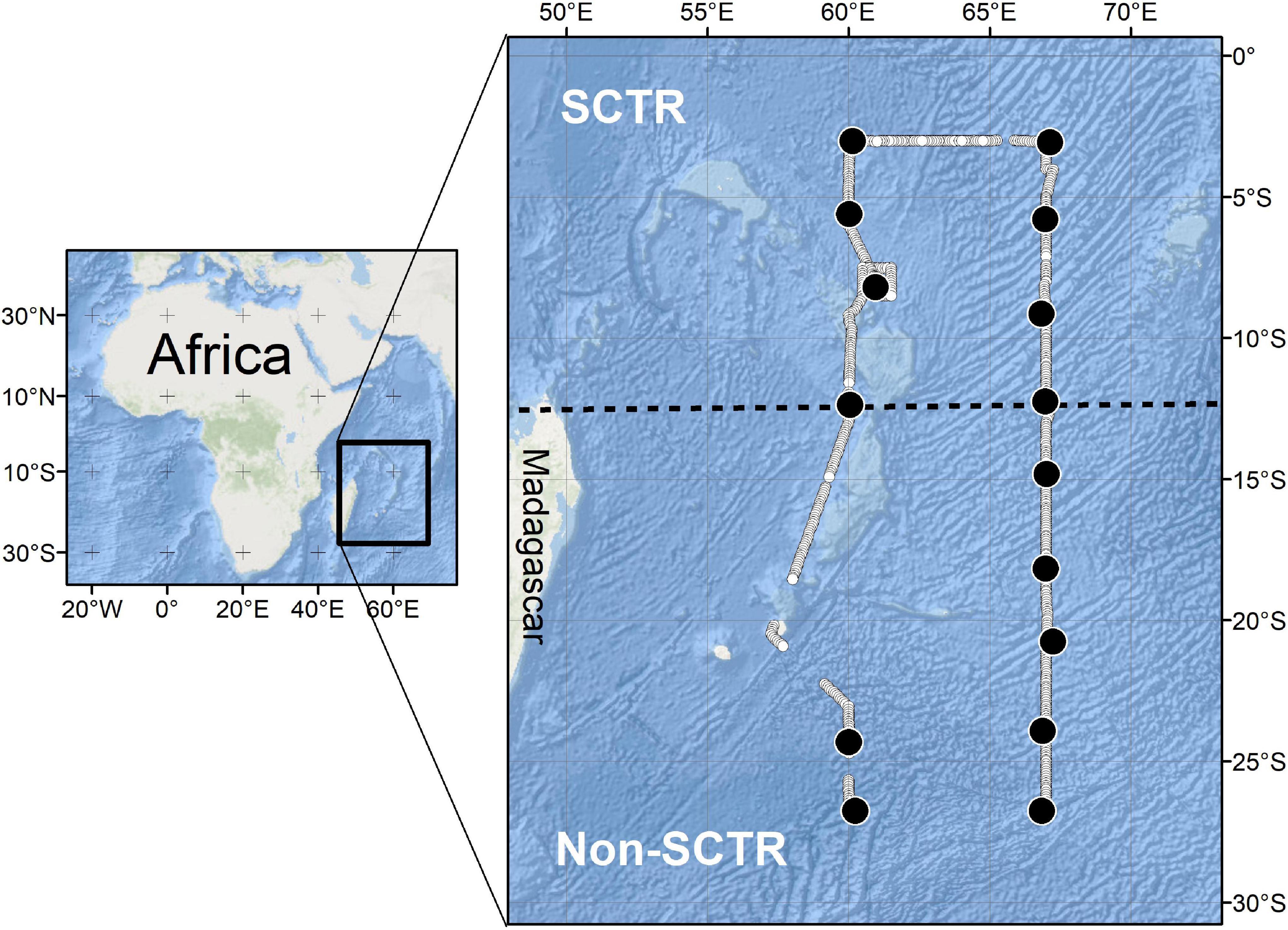
Figure 1. The study area. The line composed of white closed circles is the voyage track. The region north of 12°S is defined as Seychelles-Chagos Thermocline Ridge (SCTR) and that south of 12°S is called as non-SCTR. The black dot indicates the station of MOCNESS. The location of the CTD station is not displayed but is every degree of latitude between 3°S and 27°S at 60°E and 67°E longitude, respectively.

A conductivity-temperature-depth (CTD) probe (SBE 911plus, Sea-Bird Scientific) was used to obtain the hydrographic (physical and biogeochemical) water properties such as water temperature, salinity, dissolved oxygen, and chlorophyll fluorescence. A total of 39 CTD vertical profiling data were collected from approximately 3°S to 27°S at 60°E and 67°E. The CTD data were quality controlled and assured via typical processing methods, and the marine environmental (hydrographic) quantities were derived using the Gibbs SeaWater Oceanographic Toolbox of TEOS-10 (McDougall et al., 2009) and averaged over 1 m vertically.

The Multiple Opening/Closing Net and Environmental Sensing System (MOCNESS) was used to collect biological samples such as zooplankton. The area of the net mouth was 1 m², and the mesh size of the net was 200 μm. The water depth layers for targeted sampling (0–40, 40–120, 120–200, 200–400, 400–600, 600–800, 800–1,000, and 1,000–2,000 m) were determined based on the water depth of the seabed at each station. A total of 15 biological sampling stations were included, of which eight were within the SCTR and seven were in the non-SCTR region (Figure 1). All samples from the discrete sampling depths were fixed with 5% neutral-buffered formalin on board. In the laboratory, they were identified to the lowest possible taxonomic level and enumerated using a stereomicroscope, according to the guidelines of Chihara and Murano (1997) and Conway et al. (2003). Their sizes were measured, using the ZEN software program (v. 3.1 Zeiss, Oberkochen, Germany), from snapshots taken with a stereomicroscope camera (AxioCam ICc5, Zeiss, Oberkochen, Germany) attached to a stereomicroscope (SteREO Discovery. V8; Zeiss, Oberkochen, Germany). The total dry biomass of samples in the depth layers at each station was measured for comparison with a categorized acoustic scatterer (crustacean/small non-swim bladder fish). Ten dominant species at each station were sorted to determine their size and density.

Acoustic Data Analysis

Acoustic data were analyzed using Echoview (ver. 11, Echoview Software Pty. Ltd.). Acoustic data above 6 m were excluded from further analysis to eliminate surface noise from rough seas. Then, a feature of the “threshold offset” in Echoview was employed to remove noise signals by ring down and surface bubbles. The seabed line was set as 1,000 m and then manually inspected and modified when the seabed depth was shallower than 1,000 m. Acoustic data below the seabed line were excluded from further analysis. The signal-to-noise ratio was improved by applying noise-removal algorithms. The combination of impulse noise and transient noise removal algorithms identified higher acoustic scattering values in a given domain than the surrounding samples (Ryan et al., 2015; Echoview, 2021). To remove the transient noise at 18 kHz, samples (smoothed value) that exceeded the transient noise threshold (7 dB) were deemed to represent transient noise and were set to the 75th percentile of samples in the context window. The cleaned echograms at 18 and 38 kHz were then exported to the Echoview data file format (.evd), and the .evd files were added as raw data files in Echoview. This expedited the data processing. The minimum threshold was set to −80 dB. The thematic map, which presents the horizontal distributional map of acoustic scatterers using the nautical area scattering coefficient (NASC, m²/nm²), which indicates the acoustic scattering strength of a nautical mile squared over a defined depth, was exported in a cell (5 nm × 1,300 m) in the cleaned 38 kHz echogram for visualization. The cell is a region or a division of echogram data into a depth layer and an interval of time or distance. The NASC values using a cell size (10 nm × 10 m) in the cleaned 38 kHz echogram were exported to display the vertical distribution of acoustic scatterers. To examine the DVM of acoustic scatterers, the rising and falling times of the echo signals on the original S_V echogram (uncleaned) at 38 kHz were marked. The rising and falling times of the echo signals could be observed, although there was noise. A time and date website provided sunrise and sunset periods in Seychelles (Time and Date, 2021). To investigate the relationship between the acoustic scatterers and marine environmental properties, the echo signals in the cleaned 38 kHz echogram were selected based on the locations of the CTD stations, and then the NASC values on the selections were exported. The size of the selection was approximately 4,000 m horizontally and 1 m vertically. The NASC values at 60°E and 67°E longitude were exported to a cleaned 38 kHz echogram with a cell (30 min × 5 m) to visualize the acoustic scatterers with environmental properties.

Acoustic scatterers were categorized according to D’Elia et al. (2016), who developed an acoustic classification method for mesopelagic organisms based on length information. They used the ΔMVBS [i.e., the difference in mean volume backscattering strength (S_V, dB re 1 m²/m³) at two frequencies] method, which examines the frequency characteristics of acoustic scatterers. This method has been extensively utilized in different waters because it requires only simple mathematical equations. ΔMVBS can be expressed as:

where S_Vf1 and S_Vf2 are the mean S_Vs in a cell at 18 and 38 kHz, respectively. The cell size was 0.5 nm × 10 m, ensuring that the position and extent of each resampled value could be equivalent in two frequencies, and the frequency characteristics of acoustic scatterers could be well displayed. The ΔMVBS range was determined via the theoretical target strength (TS) models, which were used to calculate the TS difference between the two frequencies with the length information of each group. This classification was based on the minimum and maximum lengths and models of the frequency response for each group, other than certain species. Five acoustic scatterers were categorized based on the ΔMVBS range (Table 1). The acoustic categories were crustacean/small non-swim bladder fish-small (C/SNSBF-S), crustacean/small non-swim bladder fish-large (C/SNSBF-L), large non-swim bladder fish (LNSBF), swim bladder fish (SBF), and unclassified (Unc). For example, ΔMVBS ranging from 3 to 12 dB fell into the SBF in the acoustic category. After applying the given ΔMVBS ranges, S_V echograms containing only categorized acoustic scatterers were created using several operators, such as resampling by the number of pings, match ping times, match geometry, data range bitmap, and mask in Echoview (2021). The NASC values on the cleaned S_V echogram, containing each categorized acoustic scatterer, were exported for further analysis. To compare the categorized acoustic scatterer of C/SNSBF-S with the net samples from the MOCNESS, echo signals in the C/SNSBF-S echogram at 38 kHz were selected based on the position of each net sampling station, and the NASC values on the selections were exported. The size of the selection was approximately 2,000 m horizontally and 10 m vertically. The NASC values were averaged based on net sampling depth layers.

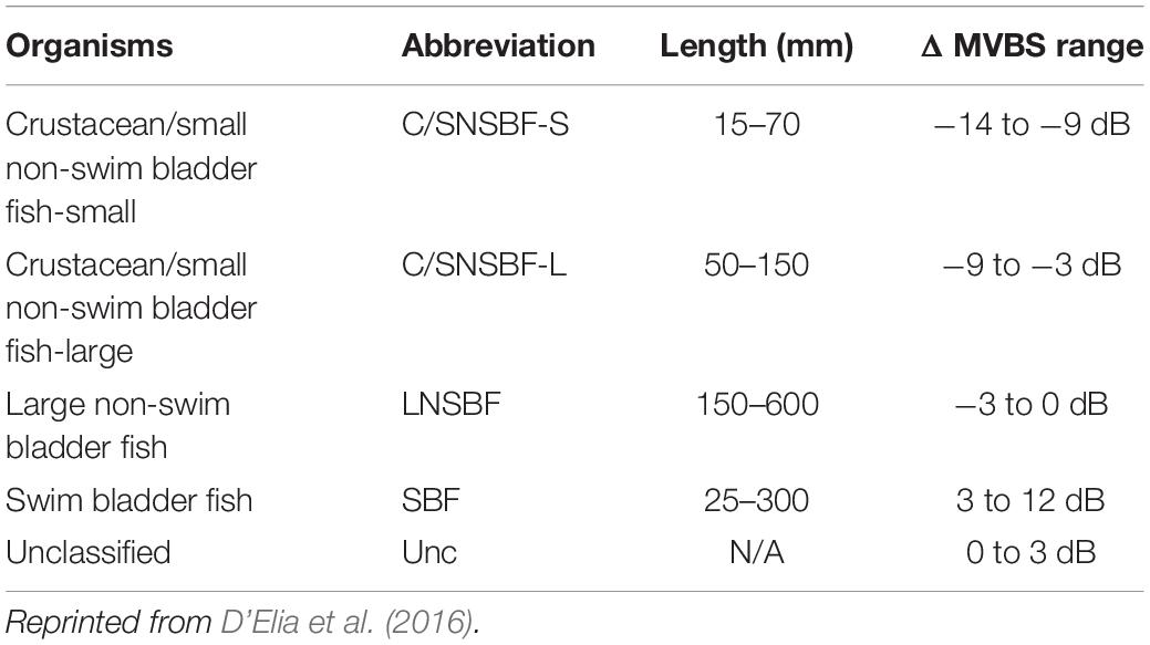
Table 1. Category of acoustic scatterers.

Nevertheless, acoustic scatterers were divided based on depth layers such as the epipelagic (E, 0–200 m), upper mesopelagic (UM, 200–600 m), and lower mesopelagic (LM, 600–1,000 m) layers. The acoustic data above 6 m were regarded as surface noise. Hence, the epipelagic layer ranged from 6 to 200 m.

Several acoustic scatterers metrics were applied (Urmy et al., 2012; Echoview, 2021). They were NASC, the center of mass (CM, the mean vertical position of the acoustic backscatter), and inertia (a metric of the spread of the acoustic backscatter around its mean location, i.e., CM). The following equations show that CM is the average of all depths sampled by weighting with their S_V values: As more backscatters move away from the CM, the inertia increases.

where z is the depth (m) of the sample in this region. S_V(z) is the volume backscattering coefficient at z.

Visualization of Acoustic Data and Environmental Properties

ArcMap (version 10.2.2., ESRI) was used to create a thematic map of the acoustic scatterers. SigmaPlot (ver 12, Systat Software Inc.) and Ocean Data View (ODV, ver 5.2.1, AWI) were used to visualize the marine environmental properties. In SigmaPlot, boxplots of the marine environmental properties were utilized based on the depth layers between the SCTR and non-SCTR. In the ODV, the data-interpolating variational analysis was applied spatially to interpolate the environmental data, considering the coastlines and bathymetry features to structure and subdivide the domain on which estimation was performed. Although the method is complex and the available CPU time and memory might be limited, it can work in arbitrary high-dimensional space, time, and depth and is a computationally advanced interpolation method (Troupin et al., 2012).

Statistical Analysis

The Mann–Whitney U-test was applied to define the statistical difference of the metrics of acoustically categorized scatterers (NASC, CM, and inertia) in each depth layer (E, UM, and LM) between the SCTR and non-SCTR. Moreover, it was also used to determine the statistical difference of the acoustically categorized scatterers (C/SNSBF-S, C/SNSBF-L, LNSBF, SBF, and UnC) in the depth layers of the SCTR and non-SCTR. The Spearman rank-order correlation coefficient was calculated using the selected NASC based on the position of the CTD station and the environmental properties (water temperature, salinity, chlorophyll fluorescence, and dissolved oxygen) with the depth layers in SCTR and non-SCTR regions to examine their correlation. Finally, the same test was used to investigate the relationship between the NASC of C/SNSBF-S and total biomass from MOCNESS. All statistical analyses were performed using the SPSS software (ver. 25, IBM).

Results

Diurnal Vertical Migration of Acoustic Scatterers

The average rising and falling times of the echo signals during the survey period were 17:10 and 5:30, respectively. The average sunset and sunrise times in Seychelles during the same period were 18:12 and 6:15, respectively. Clear DVMs were observed at depths of 200–800 m (Figure 2). Acoustic scatterers started to rise approximately 1 h before sunset in Seychelles and began to descend approximately 45 min before sunrise. The DVM of 400–800 m in the SCTR was clearer and shallower than that in non-SCTR. The entire DVM showed higher acoustic scattering values in the SCTR than in non-SCTR with stronger acoustic scatterers in the SCTR (approximately 100 m) than in the non-SCTR region.

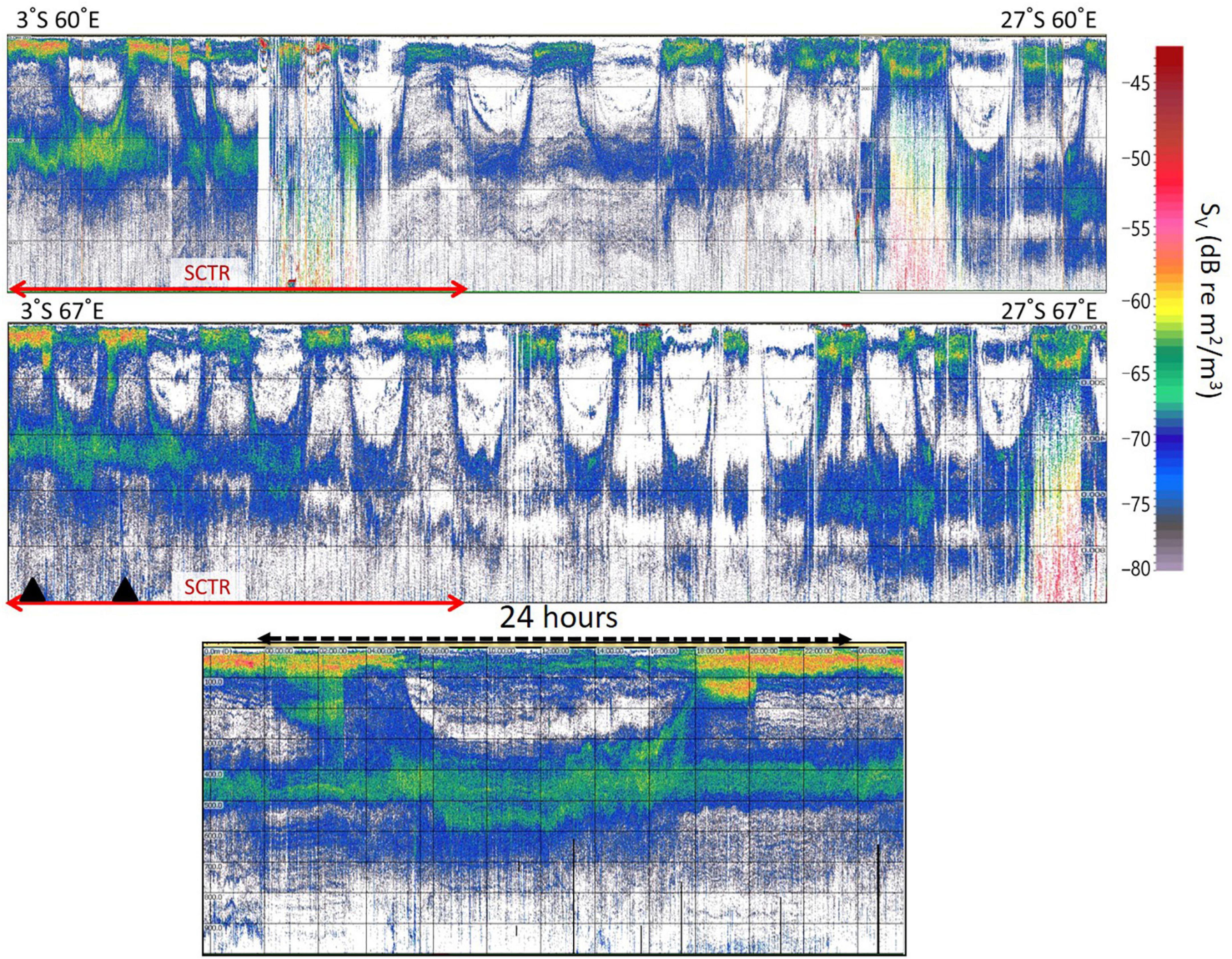
Figure 2. Diurnal migration pattern of acoustic scatterers. Clear diurnal migrations are visible in 200–800 m depth. Diurnal migration of 400–800 m in the SCTR (marked with red arrows) was clearer and shallower than that in the non-SCTR. The top echogram starts from the latitude of 3°S to 27°S in 60°E of longitude. The middle echogram begins from 3°S to 27°S in 67°E. A 24 h echogram (bottom) was recorded on May 2 of 2019 and was derived from two black triangles of the middle echogram. The horizontal lines every 200 m depth are shown in all echograms.

Thematic Map of Acoustic Scatterers

Distinctly higher NASC values were observed in the SCTR than in the non-SCTR region (Figure 3). The average NASC of the entire water column was averaged every 5 nm in the horizontal direction. The average and SD values of NASC in the SCTR were 1,401.1 ± 552.4 m²/nm² and those in non-SCTR region were 477.3 ± 288.4 m²/nm². The average NASC value in the SCTR was 2.6 times larger than that in the non-SCTR region.

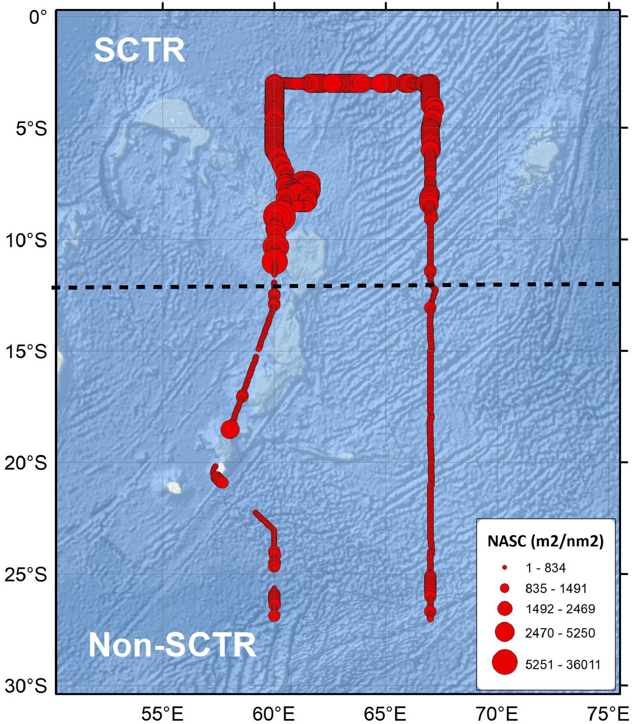
Figure 3. The thematic map of acoustic scatterers. The black dotted line is a reference line, which is 12°S, to define SCTR and non-SCTR regions.

Metrics of Categorized Acoustic Scatterers

The average and SD values of the NASC, CM, and inertia of the categorized acoustic scatterers based on the depth layers between SCTR and non-SCTR regions are listed in Table 2. The NASC value in the SCTR was much higher than that in the non-SCTR group. The CM in non-SCTR was larger than that in the SCTR, except for C/SNSBF-S of E and UM, C/SNSBF-L of all depth layers, and LNSBF of E. This means that most CMs in the non-SCTR region were deeper than those in the SCTR. The inertia in the SCTR was higher than that in the non-SCTR region, except for the Unc of E. The greatest dispersion from the CM, which is the moment of inertia, was observed at the UM in both the SCTR and non-SCTR regions. The inertia was larger in the SCTR than in the non-SCTR region, indicating that the acoustic scatterers were more diffusively distributed in the former than in the latter. The highest acoustic strength occurred at E (0–200 m) in both the SCTR and non-SCTR regions, except for the C/SNSBF of UM in the SCTR. The Mann-Whitney U-test highlighted significant differences in the NASC, CM, and inertia of categorized acoustic scatterers based on depth layers between SCTR and non-SCTR regions, except for the inertia of C/SNSBF-L of E (U(N_SCTR = 6,538, N_non–SCTR = 23,668) = 73,125,742.00, p > 0.05).

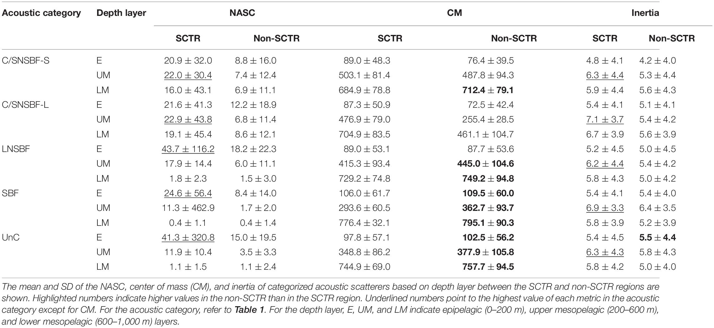
Table 2. Metrics of categorized acoustic scatterers.

Categorized Acoustic Scatterers Based on Day and Night Times

The NASC values in the categorized acoustic scatterers and depth layers were higher in the SCTR than in the non-SCTR region, except for LNSBF in LM (Figure 4). In the SCTR, the highest peak was LNSBF at 15:00 (220.9 m²/nm²), and the second-highest peak was SBF at 04:00 (152 m²/nm²) in E. In UM, the highest peak was Unc at 17:00 (84.9 m²/nm²), while that in LM, it was C/SNSBF-S at 15:00 (37.7 m²/nm²). In the non-SCTR region, the highest peak in E was C/SNSBF-S at 20:00 (40.5 m²/nm²), that in UM was C/SNSBF-S at 20:00 (21.6 m²/nm²), and that in LM was C/SNSBF-S at 02:00 (15.1 m²/nm²). In LM, C/SNSBF was dominant in both SCTR and non-SCTR regions, regardless of time. Overall, in the SCTR, high NASC in E was observed at night rather than during the daytime, while high NASC in UM and slightly high NASC in LM were found in the day rather than at night. In the non-SCTR region, high NASC in E was observed at night rather than during the day and high NASC in UM and LM were found at night. In particular, in E, LNSBF and SBF were observed in both the SCTR and non-SCTR regions. In UM, C/SNSBF and LNSBF appeared high, and in LM, high C/SNSBF occurred in both the regions. Furthermore, the Mann-Whitney U-test was performed to determine the statistical difference based on day and night for acoustic categories (C/SNSBF-S, C/SNSBF-L, LNSBF, SBF, and UnC) and among depth layers (E, UM, and LM) in SCTR and non-SCTR. The results showed a significant difference between day and night except for C/SNSBF-S in UM in the SCTR [U(N_day = 7,637, N_night = 9,091) = 34,324,863.00, p > 0.05] and C/SNSBF-S in E [U(N_day = 1,539, N_night = 2,812) = 2,144,895.00, p > 0.05) and UM [U(N_day = 4,702, N_night = 5,839) = 13,426,225.50, p > 0.05] in the non-SCTR region.

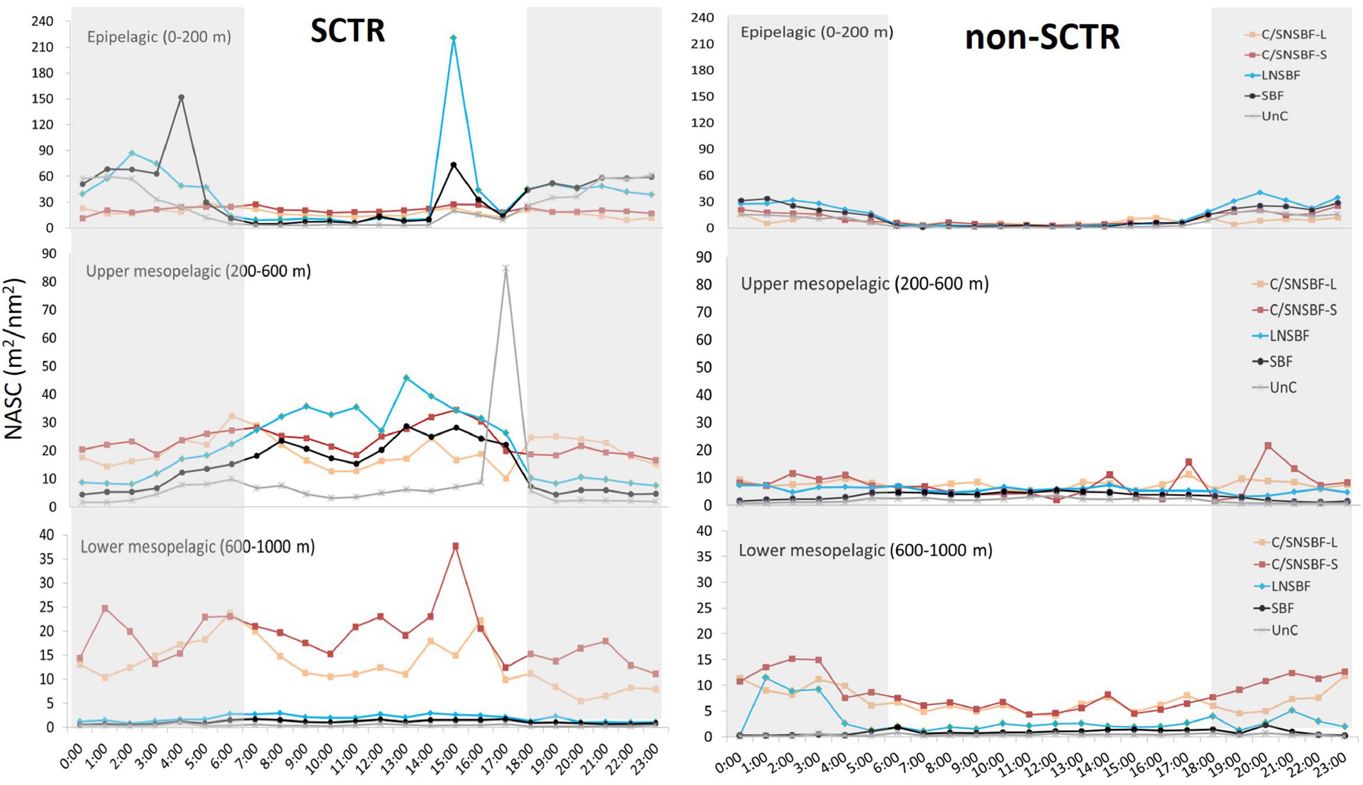
Figure 4. Categorized acoustic scatterers based on day and night times. The abbreviation of acoustic scatterers can be referred to in Table 1. Note that y-axes have different scales based on the depth layer. The gray section indicates nighttime.

Vertical Distribution of Acoustic Scatterers Based on Dawn, Day, Dusk, and Night

The acoustic scatterer profiles based on dawn, day, dusk, and night times were presented every 10 m with the entire horizontal data (Figure 5). After sunrise in the SCTR, the NASC near the water surface up to 150 m during the daytime was distinctly low. In shallow waters, the acoustic scattering value gradually increased after sunset, showing the highest value (223.6 m²/nm² at 60 m) at nighttime. The acoustic scattering value at the center of 400–500 m was relatively high (approximately 50 m²/nm²), regardless of time. The scattering value of this depth was distributed over a wider range (300–650 m) during the day than at other times. In the non-SCTR region, the NASC near the surface during daytime was also considerably low. The highest scattering value of 48.3 m²/nm² was found at 70 m at night. The acoustic scatterers centered at 400–500 m observed in the SCTR were hardly found in the non-SCTR region. Instead, a weak signal was observed at the center of 600 m.

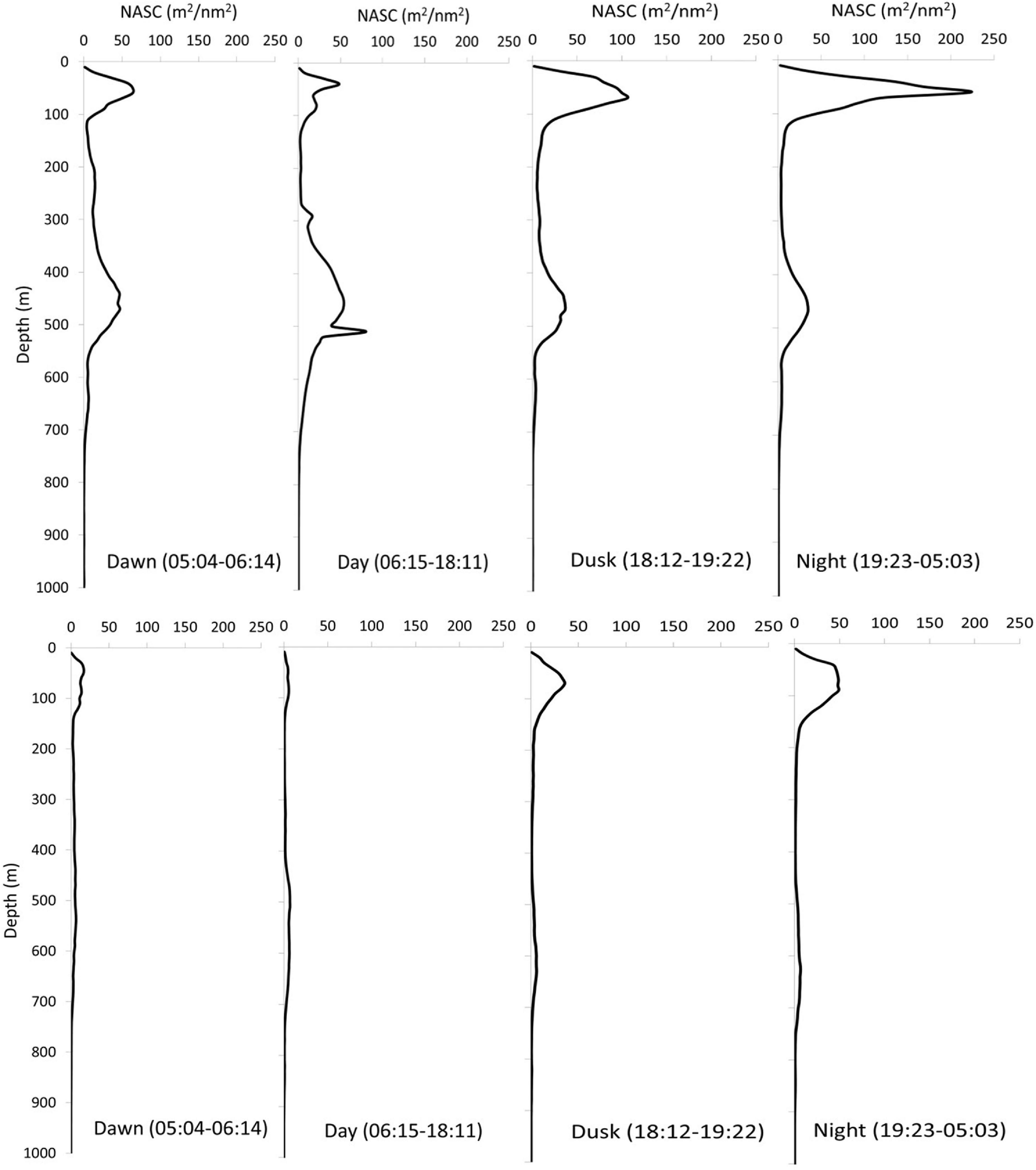
Figure 5. Vertical distribution of acoustic scatterers based on dawn, day, dusk, and night. The average sunrise and sunset times in Seychelles during the survey period were 6:15 and 18:12, respectively. The top panels correspond to SCTR and the bottom panels to non-SCTR.

Marine Environmental Properties

The marine environmental properties of the depth layers were compared between the SCTR and non-SCTR regions using boxplots (Table 3 and Figure 6). In the E category, the mean and SD values of the temperatures were 20.2 ± 5.8°C (SCTR) and 22.2 ± 3.8°C (non-SCTR). In UM, the minimum and maximum values were 7.5 and 15.0°C (SCTR) and 7.3 and 20.6°C (non-SCTR), respectively. In LM, the first and third quartiles were 6.3 and 7.5°C (SCTR), and 5.9 and 8.5°C (non-SCTR), respectively. Overall, colder waters were found in the SCTR than in the non-SCTR region. In E, the mean and SD values of salinity were 35.0 ± 0.3 psu (SCTR) and 35.3 ± 0.3 psu (non-SCTR). Many lower outliers associated with fresher water near the surface were observed in both the SCTR and non-SCTR regions. For the salinity of the UM, the mean and SD values were 34.9 ± 0.1 psu (SCTR) and 35.1 ± 0.3 psu (non-SCTR). In LM, the mean and SD values were 34.8 ± 0.1 psu (SCTR) and 34.6 ± 0.1 psu (non-SCTR). Overall, fresh water with slightly lower salinity was observed in E and UM of the SCTR than in those of the non-SCTR region. For the dissolved oxygen of E, the interquartile range in the SCTR (85.8–183.5 μmol/kg) was much wider than that of the non-SCTR region (188.5–208.2 μmol/kg), as the oxycline, where dissolved oxygen sharply varies vertically, was observed within the E in the SCTR and within the LM in the non-SCTR region. For the dissolved oxygen of the UM, the mean and SD values were 108.9 ± 21 μmol/kg (SCTR) and 207 ± 31.5 μmol/kg (non-SCTR). However, for the dissolved oxygen of the LM, the mean and SD values were 73.4 ± 7.4 μmol/kg (SCTR) and 171.8 ± 52.1 μmol/kg (non-SCTR). The interquartile range in SCTR was much narrower than that in the non-SCTR region in the LM, where the oxycline was present. Overall, water with lower dissolved oxygen levels was observed in the SCTR than in the non-SCTR region. For the chlorophyll fluorescence of E, the mean and SD values were 0.05 ± 0.39 v and 0.10 ± 0.36 v for the SCTR and non-SCTR regions, respectively. Overall, a slightly lower fluorescence was observed in the SCTR than in the non-SCTR region. In summary, colder and more fresh water with lower dissolved oxygen was found in the SCTR than in the non-SCTR region, with no significant difference in chlorophyll fluorescence, except for salinity in the LM layer.

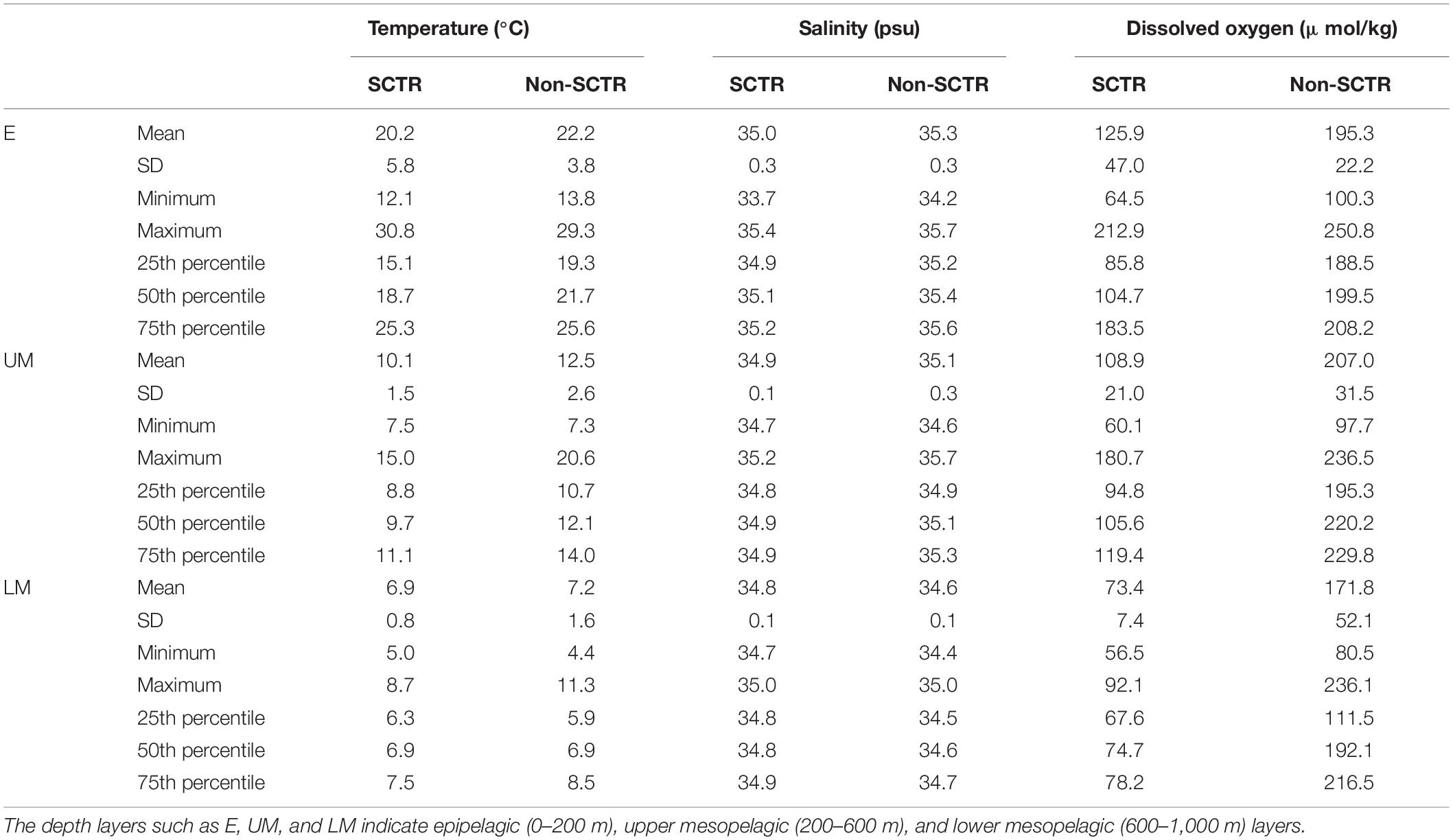
Table 3. The marine environmental properties in the depth layers between the SCTR and non-SCTR.

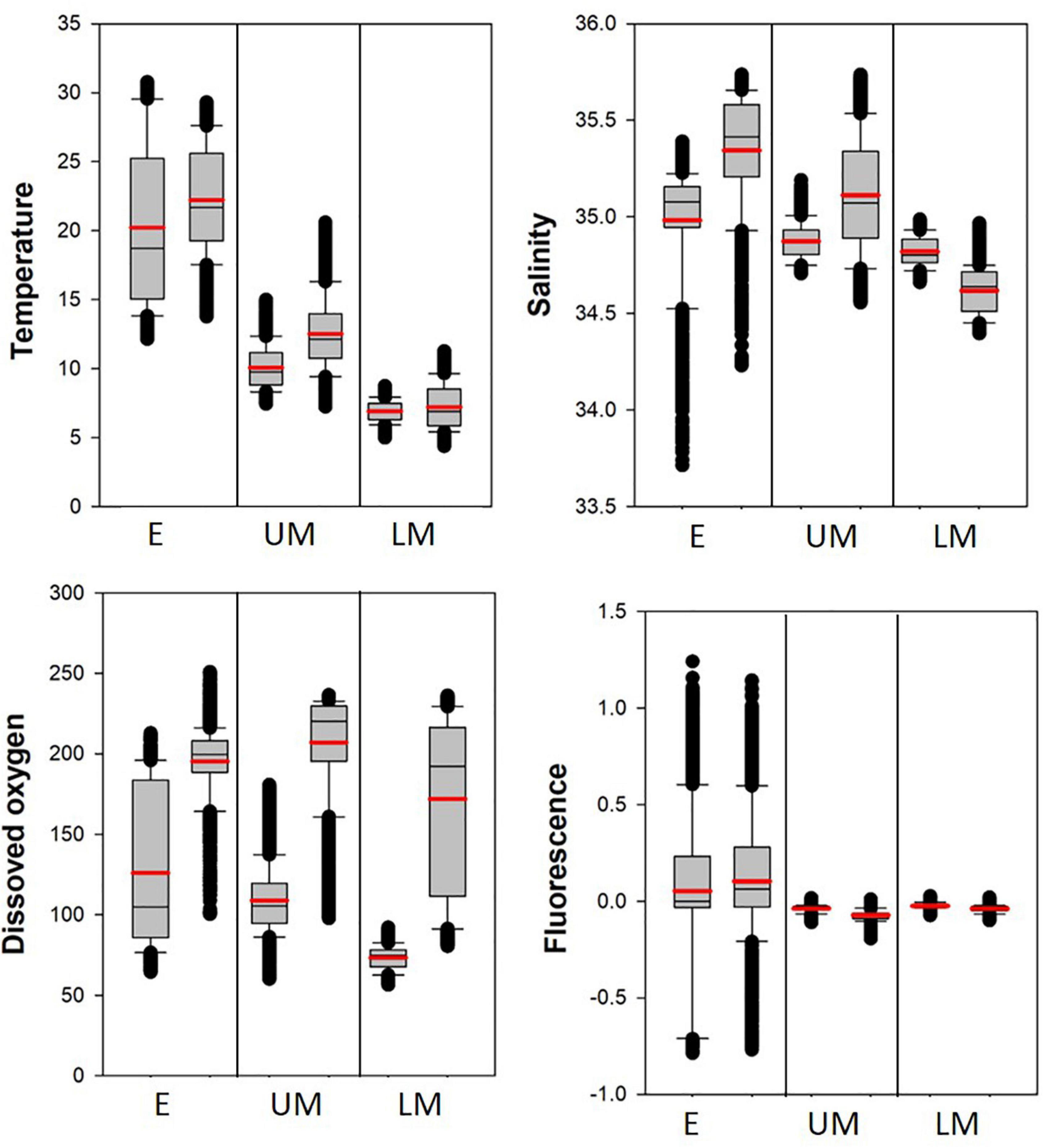
Figure 6. Boxplots of the marine environmental properties in the depth layers (E, UM, and LM) in the SCTR (first box) and the non-SCTR (second box) regions. The mean value indicates the thick red line.

Relationship Between Acoustic Scatterers and Environmental Properties

Meridional cross-sections of echograms of NASC values, temperature, salinity, and dissolved oxygen along the longitudes of 60°E and 67°E, respectively, are presented in Figure 7. Very strong acoustic scatterers were exhibited in the SCTR than in the non-SCTR region, identical to the horizontal and vertical distribution maps (Figures 3, 5). In particular, strong NASC values appeared at 400 m depth around 5°S and 60°E and along the isotherms of 9–10°C and isohalines of ∼34.90 psu. The surface water temperature ranged from 27.5 to 30°C in the SCTR and 22.5 to 30°C in the non-SCTR region. The temperature with high (>30°C) SST sharply decreased with depth within the upper 100 m and reduced to less than 12.5°C below ∼200 m in the SCTR and ∼300–500 m in the non-SCTR region. Significantly cool water in the SCTR, rather than in the non-SCTR region, was found below the thermocline. Beneath the surface freshwater [with salinity lower than 34.90 (thickness less than 100 m)], high (>34.90 psu) salinity water was found in a thin layer centered around 150 m in the SCTR, whereas a much thicker layer bordered down to ∼300–500 m was found in the non-SCTR region. For dissolved oxygen, there were at least three regimes: (1) high dissolved oxygen near the surface of both SCTR and non-SCTR and subsurface of non-SCTR, (2) low dissolved oxygen at the subsurface of SCTR, and (3) localized, enhanced/increased dissolved oxygen along the isotherms of 9–10°C and isohalines of ∼34.90 psu. In the SCTR, dissolved oxygen in the range of 125 and 200 μmol/kg appeared up to 400 m, and approximately 75 μmol/kg occurred up to 1,000 m. In the non-SCTR region, dissolved oxygen ranging from 125 to 225 μmol/kg appeared up to 400 m, and approximately 75–200 μmol/kg occurred up to 1,000 m. Overall, the dissolved oxygen in the SCTR was lower than that in the non-SCTR region.

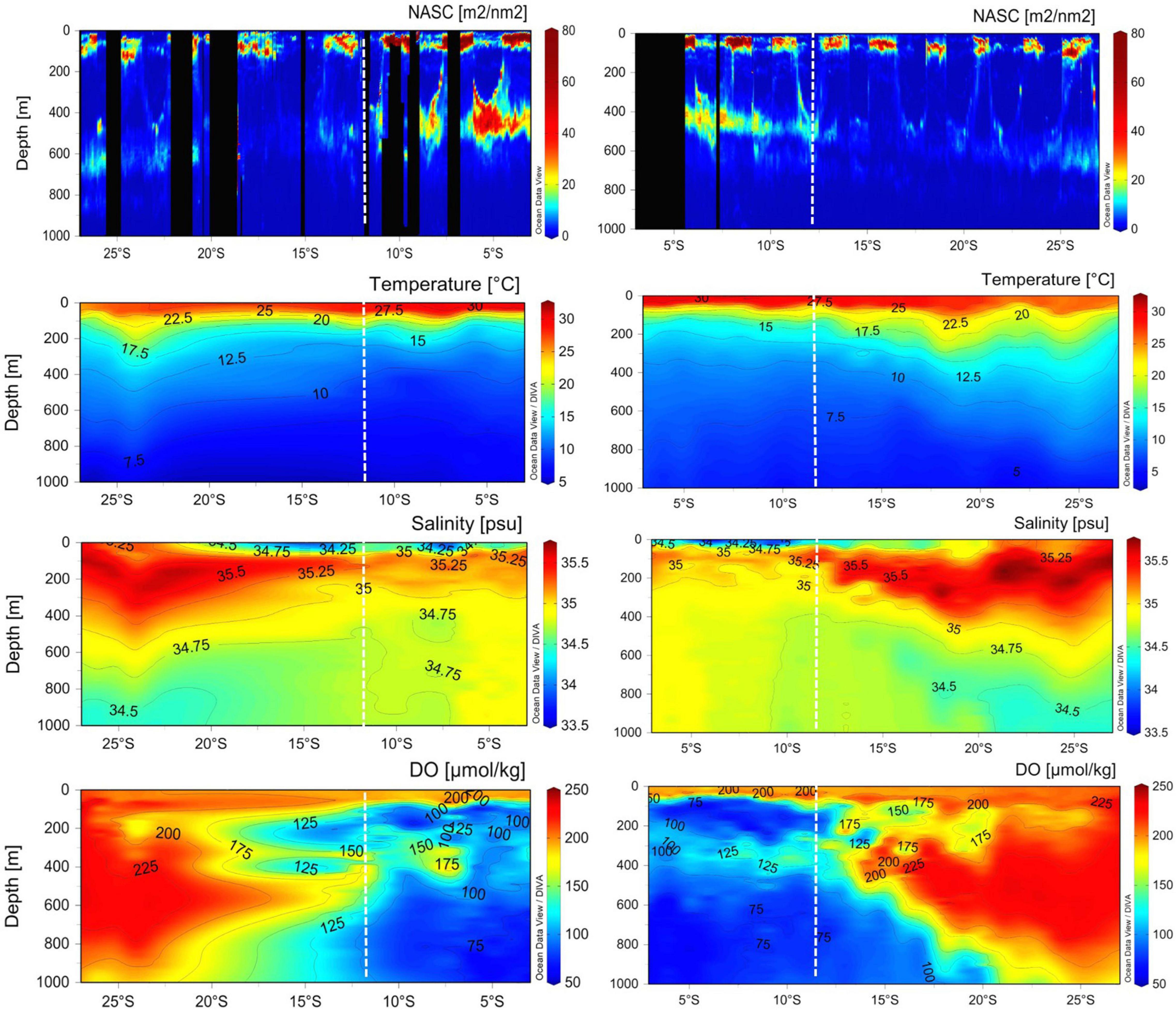
Figure 7. Meridional cross-sections of echogram, interpolated water temperature, salinity, and dissolved oxygen on 60°E longitude (left panels) and 67°E (right panels). Note that the NASC echogram was created using average NASC in a cell (30 min × 5 m) which means that it was not interpolated. The vertical black section was no-data because of heavy noise. X-axis ranges from 3°S to 27°S latitude. Contour lines with numbers are seen in environmental panels. The vertical dotted line in white in each panel indicates 12°S latitude. The SCTR extends from 3°S to 12°S, showing regions between two white dotted lines. The non-SCTR ranges from 12°S to 27°S.

The Spearman rank-order correlation coefficient was calculated between the NASC and the marine environmental (hydrographic) quantities for the depth layers in the SCTR and non-SCTR regions to examine their correlation (Table 4). The relationship between temperature and NASC showed a weak positive correlated (r_s = 0.377, p < 0.05, SCTR and r_s = 0.298, p < 0.05, non-SCTR) in E, weak negative correlated (r_s = −0.310, p < 0.05, SCTR and r_s = −0.273, p < 0.05, non-SCTR) in UM, and a strong positive correlation (r_s = 0.662, p < 0.05, SCTR and r_s = 0.763, p < 0.05, non-SCTR) in LM. A weak negative correlation between salinity and NASC was observed for all depth layers in both regions. Furthermore, there was a weak positive correlation between dissolved oxygen and NASC (r_s = 0.205, p < 0.05, SCTR and r_s = 0.172, p < 0.05, non-SCTR) in E, weak negative correlation (r_s = −0.180, p < 0.05, SCTR) in UM, and a weak positive correlation (r_s = 0.280, p < 0.05) in LM of SCTR, but a strong positive correlation (r_s = 0.620, p < 0.05) in LM of non-SCTR. There was a weak positive correlation between fluorescence and NASC in both the regions.

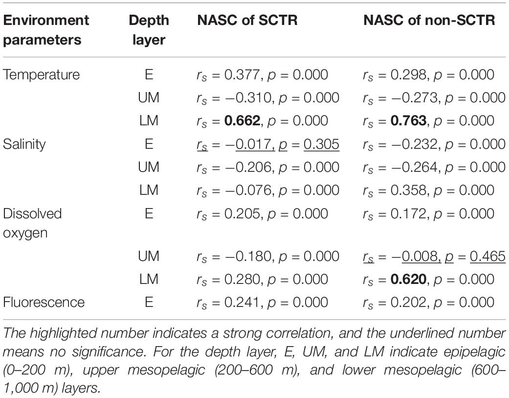
Table 4. The Spearman rank-order correlation between the NASC and the environmental parameters by the depth layer in the SCTR and non-SCTR.

Zooplankton From Multiple Opening/Closing Net and Environmental Sensing System

The species, density, and size of the top 10 dominant zooplankton from each MOCNESS station were selected and combined in each depth layer and all depth layers in the SCTR and non-SCTR regions, respectively (Table 5). In the entire water column of the SCTR, the most dominant species was Paracalanus copepodites, with a density of 75 inds./m³ ranging in 0.3–0.8 mm, followed by Pyrocystis noctiluca with 68 inds./m³ in 0.25–0.40 mm. However, in the non-SCTR region, Oncaea copepodites were the most dominant species, with a density of 42 inds./m³ ranging in 0.6–0.8 mm, followed by Ostracods with 35 inds./m³ in 0.2–2.2 mm. In the E of the SCTR, Paracalanus copepodites were the most dominant, with a density of 65 inds./m³ ranging in 0.3–0.8 mm, followed by Oncaea copepodites with 55 inds./m³ (0.6–0.8 mm). Furthermore, in the UM, the dominant taxon was Oncaea copepodites, with 7 inds./m³ ranging in 0.6–0.8 mm, followed by Ostracods with 3 inds./m³ (0.2–2.2 mm). In the LM, the most dominant taxon was Oncaea copepodites, with 4 inds./m³ ranging in 0.6–0.8 mm, followed by Speleoithona copepodites with 2 inds./m³ (0.5 mm). In contrast, in the E of the non-SCTR region, Oncaea copepodites were the dominant taxa with a density of 39 inds./m³ ranging in 0.6–0.8 mm, followed by Paracalanus copepodites with 28 inds./m³ (0.3–0.8 mm). In the UM, it was observed that the most dominant taxon was Ostracods, with 8 inds./m³ (0.2–2.2 mm), followed by Speleoithona copepodites with 4 inds./m³ (0.5 mm). Lastly, in the LM, the most dominant taxon was Speleoithona copepodites, with 8 inds./m³ (0.5 mm), followed by Speleoithona spp. with 3 inds./m³ (0.6–0.7 mm). Overall, the density of the top 10 dominant zooplankton in the SCTR was higher than that in the non-SCTR region in the epipelagic and integrated layers. The size of the numerically dominant zooplankton ranged from 0.2 to 2.9 mm in all depth layers (0–1,000 m). The immature copepods (copepodites) were the top-ranked taxa in both the SCTR and non-SCTR regions. Paracalanus copepodites were in developmental stages I–V and were grouped into one size group such as 0.3–0.8 mm. The same method was applied to other copepodites, such as Oncaea copepodites. Ostracods (0.2–2.2 mm) and foraminifera (0.2–0.4 mm) were grouped without distinction between adults and immature stages.

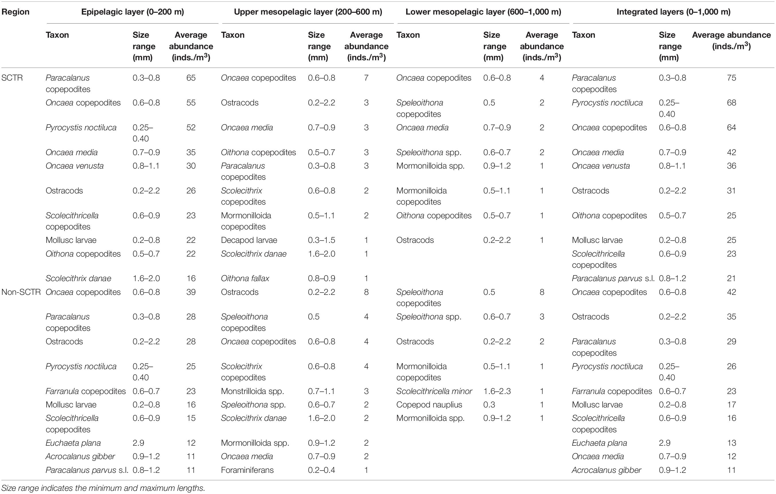
Table 5. Average abundance (inds./m³) and size range (mm) of top 10 numerical dominant zooplankton listed in decreasing order for each depth layer (epipelagic, upper mesopelagic, and lower mesopelagic) and integrated depth layers in the SCTR and non-SCTR regions.

Relationship Between Zooplankton and Categorized Acoustic Scatterers

There was no significant correlation (r_s = −0.2, p > 0.05) between the categorized acoustic scatterers (C/SNSBF-S, 15–70 mm) and the total dry zooplankton weight (mg/m³) from the MOCNESS.

Discussion

Considering the ΔMVBS Method for Acoustic Categorization

Using the ΔMVBS method in this study, we found that the ΔMVBS ranges for acoustic categorization contained all scatterers detected by the two frequencies. The “unclassified” category was named so because some organisms such as pteropods, gelatinous zooplankton, and cephalopods have insufficient length information or less developed scattering models (D’Elia et al., 2016). Generally, larger SL organisms have a smaller effect on frequency. In addition to size, organisms with density very different from that of seawater resonate well. For example, SL organisms containing either swim bladders, hard shells, or gas inclusions strongly (SBF in this study) reflect sound to the transducers. A gas bladder or pneumatophore contributes more than 95% of the total backscattering strength of an individual organism. Some organisms (C/SNSBF and LNSBF in this study) with densities similar to seawater have weak reflections (Stanton and Chu, 2000; Simmonds and MacLennan, 2005). Accordingly, different scatterers with different sizes, densities, and behavioral characteristics are expected to have different frequency responses among multiple frequencies (Kang et al., 2002, 2016, 2020). Frequency characteristics (involving frequency responses among multiple frequencies) are common means of classifying marine organisms. Generally, zooplankton have a stronger reflection at 120 kHz than at 38 kHz. Using these frequency characteristics, Antarctic krill has been frequently identified in fishes to estimate their biomass and understand their ecological properties in the Antarctic Ocean (La et al., 2016; Kang et al., 2020). Another example is that micronekton such as the gas-bearing group (ΔMVBS_120–38 < −1 dB), fluid-like group (ΔMVBS_120–38 > 2 dB), and undetermined group (−1 < ΔMVBS _120–38 < 2 dB) were discriminated in the eastern Kerguelen waters of the sub-Antarctic zone (Béhagle et al., 2017). Note that higher frequencies have a limited detection range compared to lower frequencies because the absorption coefficient of sound in water is extremely high when the frequency becomes high (Simmonds and MacLennan, 2005). In this study, disagreement between the zooplankton and categorized acoustic scatterers (C/SNSBF-S) could be resolved using higher frequencies, such as 120 kHz and more, to identify zooplankton, although the maximum detection range is limited up to 300 m for 120 kHz.

Some issues regarding the frequency response of SL organisms should be addressed. Aspects of DVM can modulate their frequency responses. Of these, mesopelagic fishes with swim bladders (SBF in this study) change their buoyancy abilities and pitch angles so that their swim bladder volumes are altered based on the water depth during DVM. Accordingly, the frequency response varies. When some taxa with gas-filled swim bladders age, the gas becomes ontogenetically fat-invested (Yasuma et al., 2010). Their gas volume does not rely on their size; therefore, their backscattering strength may significantly decrease. Subsequently, uncertainty in biomass estimation and ecological interpretation of SL organisms can potentially occur.

This was the first time that acoustic data was collected from the southwest Indian Ocean using RV Isabu, and calibration was not conducted. The echosounder was calibrated in 2020; however, the 18 kHz transducer was not calibrated, although 38 kHz was calibrated. Thus, the calibration parameters were not applied to the acoustic dataset used in this study. Backscattering values from an uncalibrated echosounder were compared with those obtained from a calibrated sounder using linear regression. Hence, the values from the two echosounders are proportional (Demer et al., 2015).

Using the ΔMVBS method, averaging samples before classifying species groups reduces random variability in the relative frequency response and minimizes bias affected by different insonified sampling volumes at different frequencies. In this study, two different beam widths (11.5° at 18 kHz and 7.1° at 38 kHz) were used, although the same pulse length (1.024 ms) was applied. This discrepancy can be compensated by averaging the samples in a cell. The criteria for selecting an optimal cell size are to maintain the morphological characteristics of classified groups and to represent their frequency characteristics, that is, the ΔMVBS pattern (Kang et al., 2002, Kang et al., 2006; Korneliussen et al., 2008). In this study, we used several cell sizes to consider this aspect.

The Center Depth Layers of the Scattering Layer Organisms

In this study, the center depth layers with high backscattering strength were approximately 100 m and 400–600 m, respectively (Figure 5). The Spanish Circumnavigation Expedition, Malaspina 2010, was conducted from December 2010 to July 2011 across three major oceans, the Pacific Ocean, the South Indian Ocean, and the Atlantic Ocean (Klevjer et al., 2016). They found that the weighted mean depth calculated from the NASC values was approximately 590 m in the southern Indian Ocean. Additionally, the epipelagic depth layer showed high NASC at night compared to the daytime. These features are consistent with our observations (the center depth of 450 m) within the SCTR, although their voyage track in the southern Indian Ocean was from South Africa to the southwest of Australia. Furthermore, several mesopelagic studies performed in the southwest Indian Ocean presented a similar center of mesopelagic depth layers, such as 400–800 m, except for shallow seamounts (Boersch–Supan et al., 2017; Annasawmy et al., 2018, 2019, 2020; Bernal et al., 2020). Of these, the closest location to our study area was the Indian South Subtropical Gyre (ISSG, 15–25°S and 55–70°E), which showed that the peak depth of backscatters was approximately 500 m during the day and 100 m at night (Annasawmy et al., 2018). The next closest places were La Pérouse and MAD-Ridge, and their centers of mesopelagic depth layers were 500–650 m and 400–700 m, respectively (Annasawmy et al., 2019). Overall, the center depth layer in the southwest Indian Ocean was in good agreement among the studies.

Regardless of the time of the day in the SCTR, some scatterers exhibited constantly in the UM, indicating that they might be non-migrant organisms (Figures 2, 5), which has been reported in many studies (Ariza et al., 2016; Romero-Romero et al., 2019). In particular, C/SNSBF seemed to be constantly distributed, irrespective of time, in the UM of the SCTR and non-SCTR regions (Figure 4). For example, in the Canary Islands, a non-migrant organism was permanently distributed around 500–600 m, while another was found between 800 and 1,000 m (Ariza et al., 2016).

Dominant Zooplankton From the Multiple Opening/Closing Net and Environmental Sensing System

This study describes broad aspects of SL organisms based on the ΔMVBS method using relatively lower frequencies, such as 18 and 38 kHz. It is extremely difficult for this method to apply relatively small-sized zooplankton because of the relationship between their sizes and wavelengths. However, we expected some degree of relationship between the backscattering strength of C/SNSBF-S and the total dry zooplankton weight, although the size of C/SNSBF-S (15–70 mm) and that of zooplankton sampled (0.2–3.0 mm) differed. They might have a predator-prey relationship, which assumes that their distribution and biomass would be linearly synchronized. However, this was not observed in the present study.

The numerically dominant adult species of Oncaea in this study included Oncaea media (0.7–0.9 mm) and Oncaea venusta (0.8–1.1 mm). The size of copepodites of Oncaea was less than 0.8 mm. According to Böttger-Schnack (2001), the size of O. venusta females ranged from 0.75 to 1.4 mm and that of the males ranged from 0.55 to 0.98 mm. The size ranges of the species in both studies were found to be similar. Moreover, P. noctiluca showed a size range of 0.25–0.4 mm, which coincided with the size range of this species (approximately 0.25 and 0.4 mm) observed by Hauslage et al. (2017).

Possible Species of Categorized Acoustic Scatterers

A clue on species of categorized acoustic scatterers in this study can be obtained from published research conducted in the southwest Indian Ocean. Two studies were performed in this area. In one study, a Bongo net (200 and 300 μm) was used at 0–200 m to sample zooplankton, and an International Young Gadoid Pelagic Trawl (IYGPT, cod end of 5 mm) was used up to a depth of 400 m to collect micronekton in ISSG and the East African Coastal Province (EAFR). In particular, in the ISSG (21°00–24°30′S and 55°00–64°50′E), which was close to the study area, the dominant species from 0 to 200 m were fish, including Myctophidae, and the second dominant species were crustaceans. The dominant species from 200 to 590 m were crustaceans, followed by fish (Annasawmy et al., 2018). In this study, in E, LNSBF and SBF were observed in the SCTR and non-SCTR regions (Figure 4). Fish, including Myctophidae, belong to these two acoustic categories, although C/SNSBF was relatively low in this study. In this study, in UM, C/SNSBF and LNSBF appeared highly. In another study, micronekton species in two seamounts (La Pérouse seamount in the ISSG and MAD-Ridge seamount in the EAFR) in the southwest Indian Ocean were studied using the IYGPT. La Pérouse seamount (19°43′S and 54°10′E) was positioned closer to the study area than Mad-Ridge. In La Pérouse, net samples up to approximately 60 m deep (on the top of the seamount) included 69% of gelatinous organisms, 20% of crustaceans, and 11% of fish. Net samples up to approximately 600 m (flank and vicinity of the seamount) contained approximately 34.2% gelatinous organisms, 30.8% fish, 23.8% crustaceans, and 12% cephalopods (Annasawmy et al., 2019). In the UM of this study, the highest peak at 17:00 was Unc, which included gelatinous organisms and cephalopods (Figure 4). In the deeper layer, a slightly different species composition was observed.

Ground-Truthing the Acoustic Backscatters

In this study, MOCNESS (200 μm mesh size of the net) was used to target zooplankton. Thus, it was nearly impossible to validate all the categorized acoustic scatterers. In many oceans worldwide, to sample SL organisms, a variety of trawl nets, such as multi nets, Hamburg plankton nets, pelagic Harstad trawls, NIWA fine mesh midwater trawls, pelagic trawls, Isaacs-Kidd Midwater trawls, bottom trawls, Harstad pelagic trawls, Matsuda–Oozeki–Hu trawls, MOCNESS midwater trawls, standard pelagic-sampling trawls, IYGP trawls, large Aakratraal pelagic trawls, and Bongo nets, have been used (Olivar et al., 2012; Dypvik and Kaartvedt, 2013; Gauthier et al., 2014; Davison et al., 2015; Prihartato et al., 2015; Gjøsæter et al., 2017; Knutsen et al., 2017; Annasawmy et al., 2018, 2019, 2020). Each sampling gear has its fishing selectivity. Although either one or two gears are used, representative samples of SL organisms may not be obtained for species composition and quantitative evaluation. Moreover, gelatinous organisms, such as siphonophores, have been significantly under-sampled because of their fragile constituents. The combined acoustic tool with net sampling is a typical method for estimating the biomass of marine organisms and understanding their ecological properties. Normally, there is good agreement between the acoustic backscatters and the weight of the specimens. However, it is very difficult to ground-truth the acoustic backscatter of SL organisms. Frequent net samplings with different mesh sizes of the cod end may be required in stratified depth layers. A promising tool is the new wideband echosounder that provides acoustic data in very high-resolution and continuous frequency response to assist in discriminating species and the distance between individuals. However, various studies using this new system are still in the preliminary stages.

Oceanographic Features in the Seychelles-Chagos Thermocline Ridge

Numerous studies have reported that cyclonic eddies leading to upwelling of nutrient-rich water contribute to high primary and secondary productivity in the epipelagic depth layer (Landry et al., 2008; Singh et al., 2015). For example, intense upwelling events frequently occur in the Strait of Messina in the central Mediterranean Sea and significantly increase primary production (Azzaro et al., 2011). Upwelling of nutrient-rich deeper water leads to high concentrations of secondary consumers, such as the blue jack mackerel Trachurus picturatus, in the Strait because of its effect on the assemblage structure of the zooplankton and micronekton (Battaglia et al., 2016; Marsac, 2018). In the southwest Indian Ocean, micronekton backscatter was greater within the cyclone, causing upwelling in the MAD-Ridge (Annasawmy et al., 2020). Accordingly, tertiary consumers, such as the tuna species Thunnus alalunga, Thunnus obesus, Thunnus albacares, and Katsuwonus pelamis, were found in the upwelling area. This study also exhibited a much higher acoustic backscattering strength in the SCTR with upwelling features than that in the non-SCTR region (Figures 3, 5). Acoustic backscattering strength showed strong or weak correlations with environmental properties depending on other factors not considered in this study, which is beyond our objectives. However, two distinct and contrasting oceanographic features were found between the SCTR and non-SCTR regions. The SCTR would be more favorable for not only primary production but also for higher consumers than the non-SCTR region.

The thermocline, expressed as a depth of 20°C isotherms (D20), was approximately 100 m in the SCTR and 100–200 m in the non-SCTR region (Figure 7). The SST found in La Pérouse in the southwest Indian Ocean ranged from 23 to 24°C with a thermocline placed at a depth of 152–181 m in late September of 2016 (Annasawmy et al., 2020). The years of 2016 and 2019 had a positive IOD (pIOD) event, and the combination of El Niño and pIOD enhanced upwelling in the eastern tropical Indian Ocean and downwelling in the SCTR (Wang and Cai, 2020; Zhang and Han, 2020). Accordingly, the SST is expected to be higher than that in the negative and neutral IOD years, and the thermocline might be deeper than that in other IOD events. SCTR upwelling is strongly affected by climate variabilities, such as IOD and ENSO. For example, when a negative IOD event occurs in the western Indian Ocean, the tuna catch rate increases because of the decrease in SST and the increase in primary and secondary productivity, and the opposite occurs during a positive IOD event (Lan et al., 2012). The high tuna catch was recorded in the Indian Ocean during La Niña years; for instance, 1,191,828 tons of tuna landed in 2010, a strong La Niña year. The unique location of SCTR is a key region for global pelagic food webs and climate variability as well as for bio-economic fisheries. However, from 2090 to 2100, future mesopelagic backscatter in the Indian Ocean is predicted to decrease using a model of NEMO-MEDUSA-2.0, with environmental factors such as surface primary productivity, temperature, and wind stress (Proud et al., 2017). More precise information on biomass and ecological characteristics and connections with oceanographic environmental features are required to maintain the biomass of mesopelagic organisms in the southwest Indian Ocean and manage them sustainably. This study provides some of this information, however, more details about the ground-truth of SL organisms at finer scales in the southwest Indian Ocean and the SCTR are needed for a better understanding of the organisms and their surrounding environmental features.

Conclusion

This study demonstrated for the first time that distinctly different distributional dynamics (diurnal vertical migration pattern, horizontal and vertical distributions, assemblage pattern, acoustic scattering values, and biological abundance) of SL organisms within and beyond SCTR are closely associated with oceanographic features. Accordingly, various spatial distributional characteristics of SL organisms can be structured based on physical oceanographic forces. However, how SL organisms respond to the ongoing changes in physical oceanographic features affected by increased ocean warming remains to be elucidated. With increase in ocean temperature and related ecosystem changes, a vessel-based scientific echosounder can provide an efficient means to investigate the dependency of SL organisms on the physical oceanographic properties of epi- and mesopelagic depth layers. Continued and regular acoustic surveys and ground-truthing collections of epi- and mesopelagic organisms in the southwest Indian Ocean with environmental properties, such as temperature, salinity, nutrients, and prey availability, are needed. These surveys shall address both the seasonal and year-to-year variability of this community and its response to the effects of climate change. The response of SL organisms and their distributional dynamics to seasonal and annual variations remains to be seen. A potential solution is using a moored echosounder for long periods at a single site to collect continuous information on the biological and physical oceanographic characteristics of the water column. This approach would be useful for acoustically describing the dynamics of SL organisms over a broad temporal scale and explaining their responses to climate change.

Data Availability Statement

All datasets used in this study are available upon request from the first author MK (mk@gnu.ac.kr) or the corresponding author D-JK (djocean@kiost.ac.kr).

Author Contributions

D-JK conceived this study. D-JK, J-HK, MJK, SN, and YC collected the data. MK, J-HK, and MJK analyzed the data. MK wrote the manuscript. All authors contributed to the article and approved the submitted version.

Funding

This work was supported by KIOST, funded by the Ministry of Oceans and Fisheries (MOF), South Korea, through the joint application program of research vessel in 2020 (PE99885 and PE99794). Also, this research was a part of the project titled “Extracting fish ecological features in the Arctic Ocean using broadband acoustic technology,” funded by the Korean Ministry of Oceans and Fisheries (1525011758), and partially supported by KIOST Indian Ocean Study (KIOS), as part of “Biogeochemical cycling and marine environmental change studies (PE99912).”

Conflict of Interest

The authors declare that the research was conducted in the absence of any commercial or financial relationships that could be construed as a potential conflict of interest.

Publisher’s Note

All claims expressed in this article are solely those of the authors and do not necessarily represent those of their affiliated organizations, or those of the publisher, the editors and the reviewers. Any product that may be evaluated in this article, or claim that may be made by its manufacturer, is not guaranteed or endorsed by the publisher.

Acknowledgments

We acknowledge the support and dedication of all crew members of RV Isabu in completing the field survey, particularly Donjin Ham, for taking care of acoustic data.

References

Aksnes, D. L., Røstad, A., Kaartvedt, S., Martinez, U., Duarte, C. M., and Irigoien, X. (2017). Light penetration structures the deep acoustic scattering layers in the global ocean. Sci. Adv 3:e160246. doi: 10.1126/sciadv.1602468
Anderson, T. R., Martin, A. P., Lampitt, R. S., Trueman, C. N., Henson, S. A., and Mayor, D. J. (2019). Quantifying carbon fluxes from primary production to mesopelagic fish using a simple food web model. ICES J. Mar. Sci. 76, 690–701. doi: 10.1093/icesjms/fsx234
Annasawmy, P., Ternon, J. F., Cotel, P., Cherel, Y., Romanov, E. V., Roudaut, G., et al. (2019). Micronekton distributions and assemblages at two shallow seamounts of the south–western Indian Ocean: insights from acoustics and mesopelagic trawl data. Prog. Ocean 178, 102–161. doi: 10.1016/j.pocean.2019.102161
Annasawmy, P., Ternon, J. F., Lebourges–Dhaussy, A., Roudaut, G., Cotel, P., Herbette, S., et al. (2020). Micronekton distribution as influenced by mesoscale eddies, Madagascar shelf and shallow seamounts in the south–western Indian ocean: an acoustic approach. Deep Sea Res. Part II Top. Stud. Oceanogr. 176:104812. doi: 10.1016/j.dsr2.2020.104812
Annasawmy, P., Ternon, J. F., Marsac, F., Cherel, Y., Béhagle, N., Roudaut, G., et al. (2018). Micronekton diel migration, community composition and trophic position within two biogeochemical provinces of the South West Indian Ocean: insight from acoustics and stable isotopes. Deep Sea Res. I. 138, 85–97. doi: 10.1016/j.dsr.2018.07.002
Ariza, A., Landeira, J. M., Escánez, A., Wienerroither, R., de Soto, N. A., Røstad, A., et al. (2016). Vertical distribution, composition and migratory patterns of acoustic scattering layers in the Canary Islands. J. Mar. Syst. 157, 82–91. doi: 10.1016/j.jmarsys.2016.01.004
Azzaro, F., Decembrini, F., Raffa, F., and Crisafi, E. (2011). Relationship of Yearly Changes of Phytoplanktonic Fluorescence to Upwelling in the Straits of Messina. Oceanography. Marine Research at CNR. 1455–1468. Available online at: https://issuu.com/cnr-dta/docs/oceanography (accessed December 16, 2011).
Battaglia, P., Andaloro, F., Esposito, V., Granata, A., Guglielmo, L., Guglielmo, R., et al. (2016). Diet and trophic ecology of the lanternfish Electronarisso (Cocco 1829) in the Strait of Messina (central Mediterranean Sea) and potential resource utilization from the Deep Scattering Layer (DSL). J. Mar. Syst. 159, 100–108. doi: 10.1016/j.jmarsys.2016.03.011
Béhagle, N., Cotté, C., Lebourges–Dhaussy, A., Roudaut, G., Duhamel, G., Brehmer, P., et al. (2017). Acoustic distribution of discriminated micronektonic organisms from a bi–frequency processing: the case study of eastern Kerguelen oceanic waters. Prog. Ocean 156, 276–289. doi: 10.1016/j.pocean.2017.06.004
Bernal, A., Toresen, R., and Riera, R. (2020). Mesopelagic fish composition and diets of three myctophid species with potential incidence of microplastics, across the southern tropical gyre. Deep Sea Res. II 179:104706. doi: 10.1016/j.dsr2.2019.104706
Bianchi, D., Stock, C., Galbraith, E. D., and Sarmiento, J. L. (2013). Diel vertical migration: ecological controls and impacts on the biological pump in a one-dimensional ocean model. Glob. Biogeochem. Cyc. 27, 478–491. doi: 10.1002/gbc.20031
Boersch–Supan, P. H., Rogers, A. D., and Brierley, A. S. (2017). The distribution of pelagic sound scattering layers across the southwest Indian Ocean. Deep Sea Res. II 136, 108–121. doi: 10.1016/j.dsr2.2015.06.023
Boswell, K. M., D’Elia, M., Johnston, M. W., Mohan, J. A., Warren, J. D., Wells, R. J., et al. (2020). Oceanographic structure and light levels drive patterns of sound scattering layers in a low–latitude oceanic system. Front. Mar. Sci. 7:51. doi: 10.3389/fmars.2020.00051
Böttger-Schnack, R. (2001). Taxonomy of Oncaeidae (Copepoda, Poecilostomatoida) from the Red Sea. II. Seven species of Oncaea s.str. Bull. Nat. Hist. Mus. Lond. (Zool.) 67, 25–84.
Burns, J. M., and Subrahmanyam, B. (2016). Variability of the seychelles–chagos thermocline ridge dynamics in connection with ENSO and Indian Ocean Dipole. IEEE Geosci. Remote Sens. Lett. 13, 2019–2023.
Catul, V., Gauns, M., and Karuppasamy, P. K. (2011). A review on mesopelagic fishes belonging to family Myctophidae. Rev. Fish Biol. Fish. 21, 339–354. doi: 10.1007/s11160-010-9176-4
Cherel, Y., Romanov, E. V., Annasawmy, P., Thibault, D., and Ménard, F. (2020). Micronektonic fish species over three seamounts in the southwestern Indian Ocean. Deep Sea Res. II 176:104777. doi: 10.1016/j.dsr2.2020.104777
Chihara, M., and Murano, M. (1997). An Illustrated Guide to Marine Plankton in Japan. Tokyo: Tokai University Press.
Cisewski, B., Hátún, H., Kristiansen, I., Hansen, B., Larsen, K. M. H., Eliasen, S. K., et al. (2021). Vertical migration of pelagic and mesopelagic scatterers from ADCP backscatter data in the Southern Norwegian Sea. Front. Mar. Sci. 7:542386. doi: 10.3389/fmars.2020.542386
Conway, D. V., White, R. G., Hugues-Dit-Ciles, J., Gallienne, C. P., and Robins, D. B. (2003). Guide to the Coastal and Surface Zooplankton of the South-Western Indian Ocean. Occasional Publication of the Marine Biological Association 15. Plymouth: Marine Biological Association of the United Kingdom.
D’Addezio, J. M., and Subrahmanyam, B. (2018). Evidence of organized intraseasonal convection linked to ocean dynamics in the Seychelles–Chagos thermocline ridge. Clim. Dyn. 51, 3405–3420.
Danckwerts, D. K., McQuaid, C. D., Jaeger, A., McGregor, G. K., Dwight, R., Le Corre, M., et al. (2014). Biomass consumption by breeding seabirds in the western Indian Ocean: indirect interactions with fisheries and implications for management. ICES J. Mar. Sci. 71, 2589–2598. doi: 10.1093/icesjms/fsu093
Davison, P., Lara–Lopez, A., and Koslow, J. A. (2015). Mesopelagic fish biomass in the southern California current ecosystem. Deep Sea Res. II 112, 129–142. doi: 10.1016/j.dsr2.2014.10.007
D’Elia, M., Warren, J. D., Rodriguez–Pinto, I., Sutton, T. T., Cook, A., and Boswell, K. M. (2016). Diel variation in the vertical distribution of deep–water scattering layers in the Gulf of Mexico. Deep Sea Res. I Oceanogr. Res. Pap. 115, 91–102. doi: 10.1016/j.dsr.2016.05.014
Demer, D. A., Berger, L., Bernasconi, M., Bethke, E., Boswell, K., Chu, D., et al. (2015). Calibration of acoustic instruments. ICES Coop. Res. Rep. 326:133.
Dypvik, E., and Kaartvedt, S. (2013). Vertical migration and diel feeding periodicity of the skinnycheek lanternfish (Benthosema pterotum) in the Red Sea. Deep Sea Res. I. Oceanogr. Res. Pap. 72, 9–16. doi: 10.1016/j.dsr.2012.10.012
Echoview. (2021). Help File for Echoview. Available online at: https://support.echoview.com/WebHelp/Echoview.htm (accessed April 10, 2020).
Gauthier, S., Oeffner, J., and O’Driscoll, R. L. (2014). Species composition and acoustic signatures of mesopelagic organisms in a subtropical convergence zone, the New Zealand Chatham Rise. Mar. Ecol. Prog. Ser. 503, 23–40. doi: 10.3354/meps10731
Geoffroy, M., Daase, M., Cusa, M., Darnis, G., Graeve, M., Santana Hernández, N., et al. (2019). Mesopelagic sound scattering layers of the high arctic: seasonal variations in biomass, species assemblage, and trophic relationships. Front. Mar. Sci. 6:364. doi: 10.3389/fmars.2019.00364
Gjøsæter, H., Ingvaldsen, R., and Christiansen, J. S. (2020). Acoustic scattering layers reveal a faunal connection across the Fram Strait. Prog. Ocean 185:102348. doi: 10.1016/j.pocean.2020.102348
Gjøsæter, H., Wiebe, P. H., Knutsen, T., and Ingvaldsen, R. B. (2017). Evidence of diel vertical migration of mesopelagic sound–scattering organisms in the Arctic. Front. Mar. Sci. 4:332. doi: 10.3389/fmars.2017.00332
Gjøsaeter, J., and Kawaguchi, K. (1980). A Review of the World Resources of Mesopelagic Fish. FAO Fisheries Technical Paper. 193. Rome: FAO.
Grimaldo, E., Grimsmo, L., Alvarez, P., Herrmann, B., MøenTveit, G., Tiller, R., et al. (2020). Investigating the potential for a commercial fishery in the Northeast Atlantic utilizing mesopelagic species. ICES J. Mar. Sci. 77, 2541–2556. doi: 10.1093/icesjms/fsaa114
Hauslage, J., Cevik, V., and Hemmersbach, R. (2017). Pyrocystis noctiluca represents an excellent bioassay for shear forces induced in ground-based microgravity simulators (clinostat and random positioning machine). NPJ Microgr. 3, 1–7. doi: 10.1038/s41526-017-0016-x
Irigoien, X., Klevjer, T. A., Røstad, A., Martinez, U., Boyra, G., Acuña, J. L., et al. (2014). Large mesopelagic fishes biomass and trophic efficiency in the open ocean. Nat. Commun. 5, 1–10. doi: 10.1038/ncomms4271
Jaquemet, S., Ternon, J. F., Kaehler, S., Thiebot, J. B., Dyer, B., Bemanaja, E., et al. (2014). Contrasted structuring effects of mesoscale features on the seabird community in the Mozambique Channel. Deep Sea Res. II. Oceanogr. Res. Pap. 100, 200–211. doi: 10.1016/j.dsr2.2013.10.027
Jennings, S., and Collingridge, K. (2015). Predicting consumer biomass, size–structure, production, catch potential, responses to fishing and associated uncertainties in the world’s marine ecosystems. PLoS One 10:e0133794. doi: 10.1371/journal.pone.0133794
Kaartvedt, S., Staby, A., and Aksnes, D. L. (2012). Efficient trawl avoidance by mesopelagic fishes causes large underestimation of their biomass. Mar. Ecol. Prog. 456, 1–6. doi: 10.3354/meps09785
Kang, M., Fajaryanti, R., Son, W., Kim, J. H., and La, H. S. (2020). Acoustic detection of krill scattering layer in the Terra Nova Bay polynya, Antarctica. Front. Mar. Sci. 7:584550. doi: 10.3389/fmars.2020.584550
Kang, M., Furusawa, M., and Miyashita, K. (2002). Effective and accurate use of difference in mean volume backscattering strength to identify fish and plankton. ICES J. Mar. Sci. 59, 794–804. doi: 10.1006/jmsc.2002.1229
Kang, M., Honda, S., and Oshima, T. (2006). Age characteristics of walleye pollock school echoes. ICES J. Mar. Sci. 63, 1465–1476. doi: 10.1016/j.icesjms.2006.06.007
Kang, M., Zhang, H., Seo, Y. I., Oh, T. Y., and Jo, H. S. (2016). Exploratory study for acoustical species identification of anchovies in the South Sea of South Korea. Thalassas 32, 91–100.
Klevjer, T. A., Irigoien, X., Røstad, A., Fraile–Nuez, E., Benítez–Barrios, V. M., and Kaartvedt, S. (2016). Large scale patterns in vertical distribution and behaviour of mesopelagic scattering layers. Sci. Rep. 6, 1–11. doi: 10.1038/srep19873
Kloser, R. J., Ryan, T. E., Young, J. W., and Lewis, M. E. (2009). Acoustic observations of micronekton fish on the scale of an ocean basin: potential and challenges. ICES J. Mar. Sci. 66, 998–1006. doi: 10.1093/icesjms/fsp077
Knutsen, T., Wiebe, P. H., Gjøsæter, H., Ingvaldsen, R. B., and Lien, G. (2017). High latitude epipelagic and mesopelagic scattering layers–a reference for future Arctic ecosystem change. Front. Mar. Sci. 4:334. doi: 10.3389/fmars.2017.00334
Korneliussen, R. J., Diner, N., Ona, E., Berger, L., and Fernandes, P. G. (2008). Proposals for the collection of multifrequency acoustic data. ICES J. Mar. Sci. 65, 982–994. doi: 10.1093/icesjms/fsn052
Kumar, B. P., Vialard, J., Lengaigne, M., Murty, V. S. N., Foltz, G. R., Mcphaden, M. J., et al. (2014). Processes of interannual mixed layer temperature variability in the thermocline ridge of the Indian Ocean. Clim. Dyn. 43, 2377–2397.
La, H. S., Lee, H., Kang, D., Lee, S. H., and Shin, H. C. (2016). Volume backscattering strength of ice krill (Euphausia crystallorophias) in the Amundsen Sea coastal polynya. Deep Sea Res. II. Top. Stud. Oceanogr. 123, 86–91. doi: 10.1016/j.dsr2.2015.05.018
Lan, K. W., Evans, K., and Lee, M. A. (2012). Effects of climate variability on the distribution and fishing conditions of yellowfin tuna (Thunnus albacares) in the western Indian Ocean. Clim. Change 119, 63–77. doi: 10.1007/s10584-012-0637-8
Landry, M. R., Decima, M., Simmons, M. P., Hannides, C. C., and Daniels, E. (2008). Mesozooplankton biomass and grazing responses to Cyclone Opal, a subtropical mesoscale eddy. Deep Sea Res. II. Top. Stud. Oceanogr. 55, 1378–1388. doi: 10.1016/j.dsr2.2008.01.005
Langbehn, T. J., Aksnes, D. L., Kaartvedt, S., Fiksen, Ø, and Jørgensen, C. (2019). Light comfort zone in a mesopelagic fish emerges from adaptive behaviour along a latitudinal gradient. Mar. Ecol. Prog. Ser. 623, 161–174. doi: 10.3354/meps13024
Li, Y., Han, W., Shinoda, T., Wang, C., Ravichandran, M., and Wang, J. W. (2014). Revisiting the wintertime intraseasonal SST variability in the tropical south Indian Ocean: impact of the ocean interannual variation. J. Phys. Ocean 44, 1886–1907. doi: 10.1175/jpo-d-13-0238.1
Marsac, F. (2018). “The Seychelles tuna fishery and climate change,” Climate Change Impacts on Fisheries and Aquaculture: A Global Analysis, Vol. 2, (New York, NY: Wiley), 523–568. doi: 10.1111/gcb.14858
McCreary, J. P. Jr., Kundu, P. K., and Molinari, R. L. (1993). A numerical investigation of dynamics, thermodynamics and mixed–layer processes in the Indian Ocean. Prog. Ocean 31, 181–244. doi: 10.1016/0079-6611(93)90002-u
McDougall, T. J., Feistel, R., Millero, F. J., Jackett, D. R., Wright, D. G., King, B. A., et al. (2009). The International Thermodynamic Equation of Seawater 2010 (teos–10): Calculation and Use of Thermodynamic Properties. Global Ship–based Repeat Hydrography Manual, IOCCP Report. Paris: UNESCO, 14.
Olivar, M. P., Bernal, A., Molí, B., Peña, M., Balbín, R., Castellón, A., et al. (2012). Vertical distribution, diversity and assemblages of mesopelagic fishes in the western Mediterranean. Deep Sea Res. I. Top. Stud. Oceanogr. 62, 53–69. doi: 10.1016/j.dsr.2011.12.014
Prihartato, P. K., Aksnes, D. L., and Kaartvedt, S. (2015). Seasonal patterns in the nocturnal distribution and behavior of the mesopelagic fish Maurolicusmuelleri at high latitudes. Mar. Ecol. Prog. Ser. 521, 189–200. doi: 10.3354/meps11139
Proud, R., Cox, M. J., and Brierley, A. S. (2017). Biogeography of the global ocean’s mesopelagic zone. Curr. Biol. 27, 113–119. doi: 10.1016/j.cub.2016.11.003
Ramirez–Llodra, E., Brandt, A., Danovaro, R., Mol, B. D., Escobar, E., German, C. R., et al. (2010). Deep, diverse and definitely different: unique attributes of the world’s largest ecosystem. J. Biol. 7, 2851–2899. doi: 10.5194/bg-7-2851-2010
Ringelberg, J. (1995). Changes in light intensity and diel vertical migration: a comparison of marine and freshwater environments. J. Mar. Biol. Assoc. U. K. 75, 15–25. doi: 10.1017/s0025315400015162
Romero-Romero, S., Choy, C. A., Hannides, C. C., Popp, B. N., and Drazen, J. C. (2019). Differences in the trophic ecology of micronekton driven by diel vertical migration. J. Limnol. Oceanogr. 64, 1473–1483. doi: 10.1002/lno.11128
Ryan, T. E., Downie, R. A., Kloser, R. J., and Keith, G. (2015). Reducing bias due to noise and attenuation in open–ocean echo integration data. ICES J. Mar. Sci. 72, 2482–2493. doi: 10.1093/icesjms/fsv121
Sato, M., and Benoit–Bird, K. J. (2017). Spatial variability of deep scattering layers shapes the Bahamian mesopelagic ecosystem. Mar. Ecol. Prog. Ser. 580, 69–82. doi: 10.3354/meps12295
Schott, F. A., Xie, S. P., and McCreary, J. P. Jr. (2009). Indian Ocean circulation and climate variability. Rev. Geophys 47, 1–46. doi: 10.1029/2007RG000245
Shilat, A., and Valinassab, T. (1998). Trial fishing for lantern fishes (Myctophids) in the Gulf of Oman (1989–1990). FAO Fish. Circ. 935:66.
Simmonds, J., and MacLennan, D. N. (2005). Fisheries Acoustics, 2nd Edn. Oxford: Blackwell Science, 437.
Singh, A., Gandhi, N., Ramesh, R., and Prakash, S. (2015). Role of cyclonic eddy in enhancing primary and new production in the Bay of Bengal. J. Sea Res. 97, 5–13. doi: 10.1016/j.seares.2014.12.002
Spear, L. B., Ainley, D. G., and Walker, W. A. (2007). ). Foraging Dynamics of Seabirds in the Eastern Tropical Pacific Ocean. OK: Cooper Ornithological Society, 99.
Stanton, T. K., and Chu, D. (2000). Review and recommendations for the modelling of acoustic scattering by fluid–like elongated zooplankton: euphausiids and copepods. ICES J. Mar. Sci. 57, 793–807. doi: 10.1006/jmsc.1999.0517
Time and Date (2021). Seychelles, Seychelles — Sunrise, Sunset, and Daylength, April 2019 for Time and Date AS. Available online at: https://www.timeanddate.com/sun/@241171?month=4and year=2019/(accessed January 12, 2021)
Troupin, C., Bartha, A., Sirjacobsc, D., Ouberdousa, M., Brankartd, J. M., Brasseurd, P., et al. (2012). Generation of analysis and consistent error fields using the data interpolating variational analysis (DIVA). Ocean Model. 5, 90–101. doi: 10.1016/j.ocemod.2012.05.002
Urmy, S. S., Horne, J. K., and Barbee, D. H. (2012). Measuring the vertical distributional variability of pelagic fauna in Monterey Bay. ICES J. Mar. Sci. 69, 184–196. doi: 10.1093/icesjms/fsr205
Vialard, J., Duvel, J. P., Mcphaden, M. J., Bouruet–Aubertot, P., Ward, B., Key, E., et al. (2009). Cirene: air–sea interactions in the Seychelles–Chagos thermocline ridge region. B. Am. Meteorol. Soc. 90, 45–61. doi: 10.1175/2008bams2499.1
Wang, G., and Cai, W. (2020). Two–year consecutive concurrences of positive Indian Ocean Dipole and Central Pacific El Niño preconditioned the 2019/2020 Australian “black summer” bushfires. Geo. Lett 7, 1–9.
Wang, Y., and McPhaden, M. J. (2017). Seasonal cycle of cross-equatorial flow in the central Indian Ocean. J. Geophs. Res. 122, 3817–3827. doi: 10.1002/2016JC012537
Yasuma, H., Sawada, K., Takao, Y., Miyashita, K., and Aoki, I. (2010). Swimbladder condition and target strength of myctophid fish in the temperate zone of the Northwest Pacific. ICES J. Mar. Sci. 67, 135–144. doi: 10.1093/icesjms/fsp218
Yokoi, T., Tozuka, T., and Yamagata, T. (2008). Seasonal variation of the Seychelles Dome. J. Clim. 21, 3740–3754. doi: 10.1175/2008JCLI1957.1
Keywords: sound scattering layer, echosounder, frequency response, Seychelles-Chagos Thermocline Ridge, southwest Indian Ocean
Citation: Kang M, Kang J-H, Kim M, Nam S, Choi Y and Kang D-J (2021) Sound Scattering Layers Within and Beyond the Seychelles-Chagos Thermocline Ridge in the Southwest Indian Ocean. Front. Mar. Sci. 8:769414. doi: 10.3389/fmars.2021.769414
Received: 02 September 2021; Accepted: 13 December 2021;
Published: 29 December 2021.
Edited by:
Ulisses Miranda Azeiteiro, University of Aveiro, PortugalReviewed by:
Gavin Macaulay, Norwegian Institute of Marine Research (IMR), NorwayLuis R. Vieira, University of Porto, Portugal
Copyright © 2021 Kang, Kang, Kim, Nam, Choi and Kang. This is an open-access article distributed under the terms of the Creative Commons Attribution License (CC BY). The use, distribution or reproduction in other forums is permitted, provided the original author(s) and the copyright owner(s) are credited and that the original publication in this journal is cited, in accordance with accepted academic practice. No use, distribution or reproduction is permitted which does not comply with these terms.
*Correspondence: Dong-Jin Kang, djocean@kiost.ac.kr